Article

Intelligent Decision-Making Analytics Model Based on MAML and Actor–Critic Algorithms

1
School of Computer Science and Engineering, Xi’an University of Technology, Xi’an 710048, China
2
Shaanxi Key Laboratory for Network Computing and Security Technology, School of Computer Science and Engineering, Xi’an University of Technology, Xi’an 710048, China
3
School of Network and Data Center, Northwest University, Xi’an 710127, China
4
International Engineering College, Xi’an University of Technology, Xi’an 710048, China
*
Author to whom correspondence should be addressed.
AI 2025, 6(9), 231; https://doi.org/10.3390/ai6090231
Submission received: 16 July 2025 / Revised: 24 August 2025 / Accepted: 2 September 2025 / Published: 14 September 2025
(This article belongs to the Section AI Systems: Theory and Applications)

Abstract

Traditional Reinforcement Learning (RL) struggles in dynamic decision-making due to data dependence, limited generalization, and imbalanced subjective/objective factors. This paper proposes an intelligent model combining the Model-Agnostic Meta-Learning (MAML) framework with the Actor–Critic algorithm to address these limitations. The model integrates the AHP-CRITIC weighting method to quantify strategic weights from both subjective expert experience and objective data, achieving balanced decision rationality. The MAML mechanism enables rapid generalization with minimal samples in dynamic environments via cross-task parameter optimization, drastically reducing retraining costs upon environmental changes. Evaluated on enterprise indicator anomaly decision-making, the model achieves significantly higher task reward values than traditional Actor–Critic, PG, and DQN using only 10–20 samples. It improves time efficiency by up to 97.23%. A proposed Balanced Performance Index confirms superior stability and adaptability. Currently integrated into an enterprise platform, the model provides efficient support for dynamic, complex scenarios. This research offers an innovative solution for intelligent decision-making under data scarcity and subjective-objective conflicts, demonstrating both theoretical value and practical potential.

1. Introduction

Intelligent decision-making systems have become critical technological infrastructure across various industries, particularly in enterprise indicator anomaly detection and complex strategic planning scenarios. These systems face fundamental challenges: the need to balance multiple conflicting objectives, adapt quickly to dynamic environments, and integrate both subjective expert knowledge and objective data analysis.
From previous research on reinforcement learning, current approaches suffer from three primary limitations [1]. First, traditional rule-based systems lack adaptability in dynamic environments and require extensive manual tuning. Second, existing reinforcement learning methods demand large training datasets and exhibit poor generalization to new scenarios. Third, decision-making frameworks often rely exclusively on either subjective expert judgment or objective data analysis, failing to achieve an optimal balance between these complementary information sources. Furthermore, the increasing complexity of real-world enterprise environments—with high-dimensional indicator spaces, non-stationary data distributions, and conflicting evaluation criteria—has further exposed the weaknesses of conventional approaches. As enterprises face increasingly dynamic market conditions and rapid technological changes, the demand for intelligent systems capable of balancing efficiency, robustness, and interpretability has become more urgent.
This paper addresses these challenges by proposing an intelligent decision-making model that integrates Model-Agnostic Meta-Learning (MAML) with the Actor–Critic algorithm, enhanced by a novel AHP-CRITIC weight quantification method. The Actor–Critic method combines the value method and policy gradient method, which can learn from two perspectives of value and policy, and has the advantages of end-to-end learning, stability, and efficiency. However, its implementation is relatively complex; it needs to maintain and train two networks (Actor and Critic) at the same time, and it is sensitive to hyperparameters [2]. MAML can effectively solve this problem. Our approach enables rapid adaptation to new decision scenarios with minimal training data while systematically balancing subjective expertise and objective data analysis. In doing so, it bridges the gap between adaptive machine learning models and structured decision-support methodologies, offering a unified framework that can operate effectively in real-world enterprise contexts.
The main contributions of our work are summarized as follows:
  • Balanced Weight Quantification: A standardized AHP-CRITIC fusion method that systematically combines subjective expert knowledge (AHP) and objective data characteristics (CRITIC) for strategy evaluation.
  • Meta-Learning Enhanced RL: Integration of the MAML framework with the Actor–Critic algorithm featuring inner-outer loop parameter optimization for rapid adaptation to new tasks.
  • Practical Validation: Comprehensive evaluation on enterprise indicator anomaly detection with a novel Balanced Performance Index (BPI) demonstrating superior efficiency and adaptability.

2. Related Work

2.1. Reinforcement Learning for Decision Making

Traditional RL algorithms have been extensively applied to decision-making problems. Actor–Critic methods combine value-based and policy-based approaches, offering end-to-end learning capabilities but requiring careful hyperparameter tuning and suffering from training instability [3]. Deep Q-Networks (DQNs) handle high-dimensional state spaces effectively but exhibit overestimation bias and low sample efficiency [4]. Proximal Policy Optimization (PPO) provides practical advantages with fewer training iterations but lacks theoretical robustness [5]. Twin Delayed Deep Deterministic Policy Gradient (TD3) addresses overestimation through double Q-networks but increases computational complexity [6]. Furthermore, reinforcement learning has shown promising results in other dynamic domains such as power converter control, where adaptive gain scheduling [7] and transfer learning [8] have been successfully applied to maintain system stability under varying operating conditions. This further motivates the integration of meta-learning and RL for rapid adaptation in enterprise decision-making scenarios.
Despite these advancements, most RL methods remain heavily reliant on large-scale training samples and often underperform when transferred to unseen environments. This limitation is particularly problematic in enterprise applications, where data collection may be costly, privacy-sensitive, or subject to distributional shifts. Moreover, pure RL-based frameworks frequently overlook the need to incorporate higher-level decision-making principles, such as multi-criteria evaluation, that are essential in strategic planning scenarios.
Research Gap: These approaches require extensive training data and demonstrate poor generalization when environments change, limiting their practical applicability in dynamic decision scenarios.

2.2. Meta-Learning Approaches

Meta-learning addresses the limitation of traditional RL by enabling rapid adaptation to new tasks. MAML learns initialization parameters that can quickly adapt to new tasks through a few gradient steps [9]. Meta-Reinforcement Learning extends these concepts to sequential decision-making, improving sample efficiency and generalization capability [10].
Recent developments have shown promise in integrating meta-learning with advanced RL architectures to accelerate learning in sparse-reward or rapidly changing environments [11]. However, most of these works remain focused on algorithmic improvements and have not been fully adapted to enterprise decision-making contexts where multiple objectives and expert knowledge must be jointly considered.
Research Gap: Existing meta-RL methods lack effective integration with multi-criteria decision frameworks, limiting their ability to handle complex real-world scenarios requiring balanced consideration of multiple conflicting objectives.

2.3. Multi-Criteria Decision Analysis

The Analytic Hierarchy Process (AHP) provides systematic approaches for incorporating expert judgment through pairwise comparisons. CRITERIA Importance Through Intercriteria Correlation (CRITIC) offers objective weight determination based on data characteristics. However, existing approaches typically employ these methods in isolation.
In practical applications, AHP ensures interpretability and expert involvement, while CRITIC emphasizes data-driven objectivity. Nevertheless, their isolated use often leads to biased or suboptimal strategies, particularly in dynamic enterprise environments where both subjective expertise and objective evidence are indispensable. Few existing studies have explored a principled integration of these two methods, and even fewer have attempted to embed such integration within adaptive learning frameworks.
Research Gap: Current multi-criteria methods fail to effectively integrate subjective expert knowledge with objective data analysis within adaptive learning frameworks, limiting their effectiveness in dynamic environments.

3. Background

3.1. Reinforcement Learning Fundamentals

Reinforcement Learning is formulated as a Markov Decision Process defined by the tuple ( S , A , R , P , γ ) . The state space S contains all possible system states s t , and the action space A includes all possible actions a t . The reward function R ( s t , a t ) R maps state-action pairs to immediate rewards, while the transition probability P ( s t + 1 s t , a t ) defines the dynamics of the environment. The discount factor γ [ 0 ,   1 ] balances the importance of immediate versus future rewards. The objective of the agent is to learn a policy π ( a t s t ) that maximizes the expected cumulative return, expressed as follows:
J θ = E π θ t = 0    γ t r t

3.2. Actor–Critic Architecture

Actor–Critic methods combine policy learning and value estimation through two neural networks. The actor network π ( a s ; θ ) parameterizes the policy by mapping states to probabilities of actions. The critic network V ( s ; ϕ ) estimates the state-value function for policy evaluation. Policy updates are guided by the advantage function
A π s t , a t = Q π s t , a t V π s t
which indicates how much better an action is compared to the baseline value of the state. Positive advantages encourage the actor to increase the probability of the chosen action, while negative values discourage it.

3.3. Meta-Learning Framework

Meta-learning aims to learn algorithms that can quickly adapt to new tasks. MAML achieves this through a two-level optimization process:
Inner Loop: Task-specific adaptation using gradient descent on task data.
Outer Loop: Meta-parameter optimization across tasks to improve adaptation capability.
This framework enables rapid learning with minimal task-specific data by leveraging cross-task knowledge transfer.

3.4. Evaluation Metrics

To evaluate performance, we define the Balanced Performance Index (BPI), which jointly considers reward and convergence time:
BPI = α × Reward normalized + 1 α × 1 Time normalized
where α [ 0 ,   1 ] is a weighting parameter. BPI addresses the multi-objective nature of decision evaluation by explicitly trading off solution quality against computational efficiency. Higher α values prioritize solution quality, while lower α values emphasize rapid convergence.

4. Algorithm

First, at the Data Layer, the Strategy Scoring Table must be populated. This table is used to evaluate the scores of different strategies against three criteria. These scores are subsequently stored in the database for later use.
At the Weight Layer, the model first calculates the weights between different strategy groups for the same criterion using the AHP (Analytic Hierarchy Process) method. It then calculates the weights between the criteria, ultimately outputting the total weights for the different strategy groups. The Critic algorithm further calculates the weights of the strategy groups. In contrast to the AHP algorithm, Critic analyzes the information-carrying capacity of the strategy groups from an objective perspective, thereby providing group weights. Finally, the model computes the comprehensive weights to evaluate the relative merits of the strategies.
Moving to the Decision Layer, based on the abnormal indicator deviation values input by the warning system, the Actor network selects an appropriate strategy action. Subsequently, the Critic network evaluates the chosen strategy, assesses its effectiveness, and performs inner-loop updates. After completing a training batch, the model conducts outer-loop updates. The model also logs strategy selections. If the abnormal indicator does not return to normal, the model continues to select or adjust strategies. Once the abnormal indicator returns to the normal range, the model outputs the final optimal strategy to address that specific abnormal indicator.
The entire process, through the combination of weight calculation, meta-learning, and reinforcement learning, ultimately outputs the optimal decision solution.

4.1. Actor–Critic Algorithm Based on MAML Framework

Actor–Critic algorithm is a reinforcement learning algorithm that combines the strategy gradient method and the value function method [2]. The algorithm consists of two main modules: Actor and Critic. Actor is a policy network capable of learning random policies. Critic is a value network used to evaluate these policies, which can reduce the variance of policy evaluation and avoid convergence to local rather than global optimal policies. The goal of the algorithm is to maximize the expected cumulative reward.
Based on the strategy gradient theorem, the gradient of a strategy can be expressed as
θ J θ = E π θ θ log π θ a t s t Q π θ s t , a t
Since it is difficult to directly estimate Q π θ s t , a t , the Actor–Critic algorithm uses the dominant function A π θ ( s t , a t ) estimated by Critic instead, so the strategy gradient is updated as
θ J θ E π θ θ log π θ a t s t A π θ s t , a t
The Critic part updates the state value function by Time Difference (TD) errors.
δ t = r t + γ V π θ s t + 1 V π θ s t
V π θ s t V π θ s t + α δ t
where α is the learning rate.
To compute the advantage function A π ( s t , a t ) , the Q-value Q π s t , a t is estimated as follows:
Q π s t , a t r t + γ V π s t + 1
The advantage function is then obtained by subtracting the estimated state value V π ( s t ) :
A π s t , a t r t + γ V π s t + 1 V π s t
This formula effectively approximates the advantage function using TD error δ t :
A π s t , a t δ t = r t + γ V π s t + 1 V π s t
The Actor then updates the policy parameters using the policy gradient, based on the feedback from the Critic:
θ θ + β θ log π θ a t s t δ t
where β is the learning rate for the policy.
Model-Agnostic Meta-Learning (MAML) is a meta-learning method based on meta-objective gradient optimization proposed by Finn et al. [9]. It is applicable to both supervised learning and reinforcement learning. The goal of the algorithm is to train task-shared meta-parameters θ , learning an initial model parameter that can quickly adapt to new tasks. When encountering a new task, only a few gradient updates are needed to the initial model parameters to achieve good performance. It is a meta-learning method for rapid adaptation to new tasks.
Given a task set T = { T 1 , T 2 , , T N } , each task T i has its own dataset D i , which is divided into a support set S i and a query set Q i . The support set S i is used to update model parameters, and the query set Q i is used to evaluate the performance of the updated model, followed by an outer-layer parameter update based on the evaluation. The intelligent decision analysis model proposed in this paper, based on the MAML framework and Actor–Critic algorithm, integrates meta-learning and reinforcement learning concepts. The goal is not to find the best parameters for the current observation but to find parameters that can broadly adapt to data sampled from different observations. The agent learns the essence of decision-making by following the reward function, achieving higher reward values and better decision-making.
(1)
Inner-loop Optimization (Task-specific updates): For each specific task, a small-step gradient update is applied using a gradient descent algorithm to optimize the model’s parameters. This process involves performing a few gradient descent steps on each task to learn model parameters that adapt to the task.
For each task T i , the model’s initial parameters θ are updated with a small gradient step using data from the support set S i . The goal of the inner-loop update is to allow the model to quickly adapt to the task.
In the inner-loop update, the task-specific gradient updates the Actor and Critic parameters for each task T i :
θ i = θ α θ L actor T i
ϕ i = ϕ α ϕ L critic T i
where α is the inner learning rate, and θ i and ϕ i are the updated Actor and Critic network parameters for task T i .
(2)
Outer-loop Optimization (Meta-update): After completing the inner-loop update, the task-adapted model parameters are fed back. Based on the performance feedback from these tasks, the global initial model parameters are updated to improve generalization for future tasks.
The goal of the outer-loop update is to adjust the initial model parameters θ based on the feedback from the query set Q i , allowing them to not only adapt to specific tasks T i but also generalize better to other tasks.
After completing the inner-loop update for all tasks, the outer-loop update calculates the average loss across multiple tasks to update the global initial parameters, making them more general for new tasks:
θ θ β θ i = 1 N    L meta T i
ϕ ϕ β ϕ i = 1 N    L meta T i
where β is the outer learning rate, and L meta T i is the meta-loss for each task. Through inner and outer gradient descent steps, the model gradually learns a set of initial parameters that allow it to quickly adapt to future tasks with minimal updates. Ultimately, the model learns generalized meta-parameters from the training tasks, enabling it to quickly adapt to new tasks and achieve better performance [12].
The pseudocode and flowchart for the algorithm are shown in Algorithm 1 and Figure 1.
Algorithm 1: Actor–Critic algorithm based on the MAML framework
Input: List of tasks val, inner learning rate inner_lr, discount factor γ , batch size batch.
Output: The optimal strategy taken.
1Initialize the parameters θ and w for π ( s ;   θ ) and V s ;   w , and initialize the state s ;
2while not converged do
3Select action a based on the current policy π ( s ;   θ ) ;
4Execute action a and observe reward r and the next state s ;
5Calculate the T D error δ , where δ = r + γ     V s ;   w V s ;   w ;
6Update the C r i t i c network by minimizing the loss L ( w ) = δ 2 to update parameter w ;
7Update the A c t o r network using the policy gradient method to update parameter θ :
θ θ + α     δ     θ   l o g   π a s ;   θ ;
8Update the state s ;
9Update the outer layer parameters:
θ θ β θ i = 1 N    L meta T i ,   ϕ ϕ β ϕ i = 1 N    L meta T i ;
10end
First, initialize the parameters of the Actor and Critic networks, as well as the environment, and obtain the initial state. Then, enter an outer loop that continues until the model converges. In each iteration of the outer loop, tasks from the task list are processed in batches. For each task in the batch, perform the inner update: copy the current model’s parameters, reset the environment, and obtain the initial state, then initialize the cumulative reward.
While the task is not complete, select an action based on the current policy, execute the action, observe the reward and the next state, calculate the TD error, update the Critic network by minimizing the squared loss of the TD error, update the Actor network using the policy gradient method, and update the current state while accumulating the reward [13]. If the task is complete, record the inner-updated parameters and the cumulative reward.
After all inner updates for each task are complete, perform the outer update: reset the gradients of the outer optimizer, calculate the average loss across all tasks, perform backpropagation, execute the optimizer step, adjust the learning rate scheduler, and update the outer parameters. Repeat the process until the model converges [14].

4.2. AHP-CRITIC Weight Quantification Method

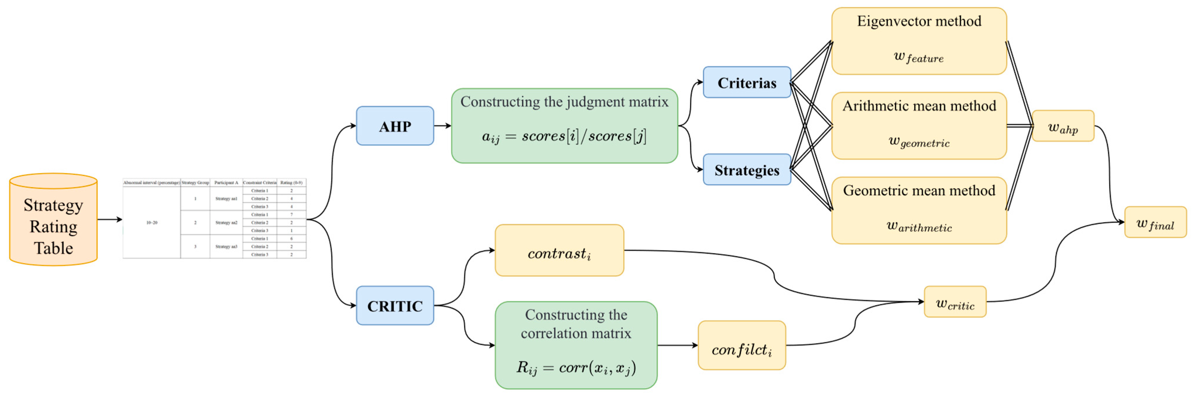
This paper takes abnormal decision-making for enterprise indicators as an example and proposes a standardized weight quantification method. First, it is necessary to fill in the professional strategy ratings in the strategy rating table. The structure of the strategy rating table is shown in Table 1 as an example. For strategies, we have three binding evaluation criteria, such as “score with great impact on target indicators”, “score with small impact on non target indicators” and “score with small implementation difficulty”. These criteria will be used to evaluate the advantages and disadvantages of strategies. The score of each constraint condition is 0–9 points. The higher the score, the more consistent this strategy is with the description of the corresponding constraint criteria. The strategy group will use this score later to calculate the AHP and CRITIC weights, and then calculate the strategy group weights.
For decision-making regarding the correction of an anomaly offset value, the offset value is divided into several intervals, with each interval containing multiple strategy groups. There are several participants in the decision, and each policy group consists of a policy provided by each participant, for which there are several constraints, such as the impact of the policy on other metrics, the impact of the policy on other participants, etc., and the expert needs to score the strategy according to these criteria in order to calculate the policy weight for the following AHP and CRITIC methods.
AHP (Analytic Hierarchy Process) can ensure the transparency and explainability of the decision-making process from a subjective point of view, combined with expert experience and judgment, while the CRITIC method can ensure the objective and scientific weight allocation, and by combining subjective evaluation and objective data analysis, it not only makes the decision-making process more systematic and rational, but also improves the sensitivity, adaptability and accuracy of the model, thereby optimizing the overall performance of the decision-making system.
(1)
The AHP method is used for multi-criterion decision analysis, which determines the weight of each criterion and scheme by constructing a judgment matrix, and converts the action plan into the form of a judgment matrix, which is a systematic data processing method, which can improve the transparency and interpretability of decision-making [15]. In this paper, AHP is used to calculate subjective strategy weights. The principle of constructing the judgment matrix is as follows:
a i j = s c o r e s i s c o r e s j
where i and j are the scores of the same constraint criteria for two different strategies being compared. a i j represents the degree of importance of strategy i relative to strategy j . If the scores of factor i and factor j are the same, then a i j = 1 .
The improved AHP method combines three weight calculation methods:
Eigenvector method: Decompose the judgment matrix A , where the eigenvector corresponding to the largest eigenvalue is the criterion weight. Let λ m a x be the largest eigenvalue, and the eigenvector w feature satisfies the following:
A   w feature = λ max w feature
Arithmetic mean method: After normalizing the judgment matrix A , the average of each row is taken as the weight. The weight vector w arithmetic satisfies the following:
w arithmetic i = 1 n j = 1 n    a i j k = 1 n a k j
Geometric mean method: Calculate the geometric mean of each row’s elements. The weight vector w geometric satisfies the following:
w geometric i = j = 1 n a i j 1 n
The final weight calculation result is the weighted average of the three methods:
w ahp = 1 3 w feature + w arithmetic + w geometric
The AHP component employs three distinct approaches—the arithmetic mean method, the geometric mean method, and the eigenvector method—to compute weights. This multi-method integration aims to synthesize weight evaluation outcomes from diverse mathematical perspectives, thereby enhancing the robustness and reliability of decision-making. The eigenvector method determines weights by solving for the eigenvector corresponding to the largest eigenvalue of the judgment matrix. Its strength lies in its strict adherence to the theoretical foundation of AHP, accurately reflecting the inherent consistency of the judgment matrix. However, a key limitation is that the results may become unstable when the consistency of the judgment matrix is poor. The arithmetic mean method calculates weights by normalizing the elements of each row in the judgment matrix and then taking the row-wise average. This approach is computationally straightforward and easy to interpret, with a reasonable tolerance to data perturbations. Nonetheless, it may overlook the nonlinear characteristics of the judgment matrix, potentially leading to overly balanced weight distributions. The geometric mean method derives weights by computing the geometric mean of each row’s elements and normalizing the results. It offers the advantage of insensitivity to extreme values and preserves ratio-scale properties. However, it cannot be directly applied when the judgment matrix contains zero or negative values.
To mitigate the potential biases introduced by any single method, the final weights are obtained by averaging the results from all three techniques. This strategy aligns with the concept of ensemble learning, reducing the limitations of individual methods while enhancing the generalizability of the weighting results. Although alternative combination strategies such as weighted averaging or principal component analysis exist, the former requires additional subjective input to determine confidence weights for each method, and the latter may compromise interpretability despite its ability to extract dominant features. Therefore, the simple averaging approach not only ensures computational efficiency but also maximizes the retention of the advantages offered by each method. This aligns with the dual objectives of balance and practicality in the AHP-CRITIC framework. Such a design also reflects the core idea of multi-method integration illustrated in Figure 2, where standardized processing harmonizes subjective judgments with objective data characteristics, ultimately forming a more adaptive and comprehensive weighting system.
(2)
The CRITIC (Criteria Importance Through Intercriteria Correlation) method is used for feature evaluation and to calculate the importance of each feature [16]. In this paper, it is used to calculate the amount of information carried by each strategy, i.e., the objective strategy weight.
Coefficient of variation: The ratio of the variance to the mean for each strategy:
contrast i = σ i 2 μ i
where σ i 2 is the variance of strategy i . And μ i = Σ k = 1 m x i , k m , it represents the mean value of strategy i on m samples, where x i , k is the k criteria scores for strategies x i .
Correlation matrix: This matrix shows the strength of linear relationships between different strategies. It is constructed by calculating the Pearson correlation coefficient between each pair of strategies, resulting in the correlation matrix R :
R i j = k = 1 n    x i , k x i ¯ x j , k x j ¯ k = 1 n    ( x i , k x i ¯ ) 2 k = 1 n    ( x j , k x j ¯ ) 2
where R i j represents the Pearson correlation coefficient between strategies x i and x j , n is the number of criteria, x i , k and x j , k are the k criteria scores for strategies x i and x j , and x i ¯ and x j ¯ are the mean values of strategies x i and x j , respectively.
Conflict: The conflict of each strategy is calculated as the sum of the absolute values of all its correlation coefficients:
conflict i = j = 1 n    R i j
Information content: The product of the coefficient of variation and the conflict:
critic i = contrast i × conflict i
Final strategy weight: Each strategy’s weight is obtained by normalizing its information content:
w critic i = critic i j = 1 n    critic j
After calculating the weight vectors from both AHP and CRITIC methods, the final strategy weight w final is determined by assigning weights to AHP and CRITIC results. The final weight is a linear combination of AHP weight and critical weight, and the weight coefficient α can be set in subsequent experiments:
w final = α · w ahp + ( 1 α ) · w critic
Figure 2 shows the calculation flowchart of w final .

5. Experiment

In this section, the goal of our experiment is to answer the following questions: (1) Can the Actor–Critic algorithm based on the MAML framework make effective decisions? (2) Is the consumption of the Actor–Critic algorithm based on the MAML framework better than that of the traditional Actor–Critic algorithm, DQN algorithm, and PG algorithm in decision-making? (3) Is the Balance Performance Index (BPI) of the Actor–Critic algorithm based on the MAML framework better than that of traditional Actor–Critic, DQN, and PG? Our code has been uploaded to Github and can be accessed from the following URL: https://github.com/Prow1er/MAC.git (accessed on 24 August 2025).
Firstly, the effectiveness of the algorithm was verified. In the case of the same low amount of training data, the offset values were randomly generated for testing to verify the effectiveness of the algorithm. Then, the effectiveness of the MAC algorithm was tested by comparing the total task reward value and the average task reward value of each algorithm under different amounts of training data, and the efficiency of the MAC algorithm was tested by comparing the time consumption. Finally, the stability and superiority of the MAC algorithm are shown by comparing the comprehensive indicators.

5.1. Experiment Setup

(1)
Calculation of Strategy Group Benefit Value
Using the strategy score table, scores for each criterion and the corresponding scores for each strategy based on the criteria are obtained. With this information, the judgment matrices for the criteria layer and the solution layer are constructed. The AHP-Critic method is applied to calculate the strategy group weight w f i n a l . Afterward, the average value of the weights for all strategies within each strategy group is computed, followed by normalization. This normalized value becomes the strategy group weight w .
Set the benefit value of the strategy group as s , the length of the anomaly interval as d , and the calculation formula of the benefit value s of the strategy group as
s = w d
(2)
Strategy Group Setup
After calculating and rounding the strategy group benefit value, the strategy group settings are determined in Table 2.
(3)
Space Settings
In this paper, the decision-making for correcting abnormal enterprise metrics is taken as an example. The anomaly interval is set to (−50, 50), and the stability interval is set to (−2, 2).
The state space is represented by a one-dimensional vector of floating-point numbers, specifically the current deviation value, which denotes the degree of deviation from a nominal value. This value ranges between a negative maximum deviation and a positive maximum deviation, as defined by the environment initialization parameters. The action space is discrete, allowing the agent to select actions from a dynamically loaded strategy library, such as strategies of type A1, B1, or C2. The number of available actions corresponds to the total number of strategies present in the strategy library.
In the environment dynamics, after the agent selects a strategy as an action in the current state, the environment queries the strategy library to retrieve the list of applicable strategies for that state. The selected strategy’s effect function is then applied to update the state. The new state value is computed deterministically, as the application of the strategy modifies the current deviation value to produce the next state. Additionally, the environment checks whether a termination condition has been met—specifically, whether the deviation value falls within a stable interval.
(4)
Reward Function Settings
Three priority levels are set. Strategies with higher benefit values are assigned higher priority and receive greater rewards. Let the reward value be r , the current anomaly value be x , and the midpoint of the stability interval be a .
First priority reward function:
r = x a 2
Second priority reward function:
r = 50 x a 2
Third priority reward function:
r = 100 x a 2
(5)
Termination Condition
The termination condition is met when the current anomaly value x enters the stability interval.
(6)
Training and Testing Data
Random anomaly values (with upper and lower bounds) are generated by fixing a random seed. The testing data consists of 100 anomaly values. Several tests are conducted with varying amounts of training data, set to 10, 20, 40, 60, 100, and 200 samples, respectively.
(7)
Network Parameter Settings
We conducted a grid search over the outer learning rate in {0.001, 0.005, 0.01}, the inner learning rate in {0.001, 0.005, 0.01}, and the meta-task size in {5, 10, 20}, and ultimately selected an outer learning rate = 0.01, inner learning rate = 0.01, and meta-task size = 5, as it performed best on the validation set. The specific parameters are shown in Table 3.

5.2. Comparative Experiments

This paper mainly compares the advantages and disadvantages of the Actor–Critic algorithm based on the MAML framework with traditional Actor–Critic algorithms and DQN algorithms.
(1)
Algorithm Validity
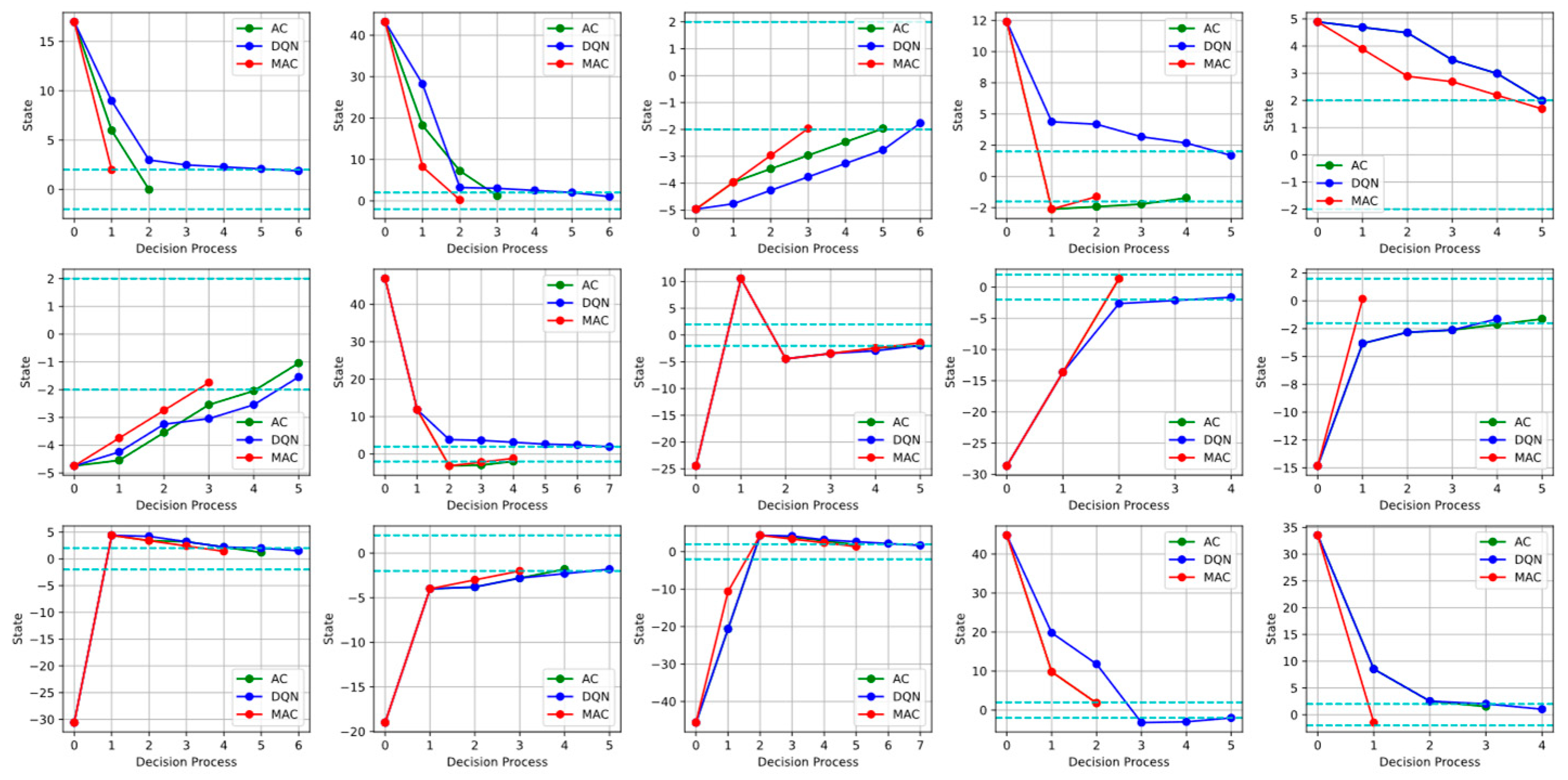
When the data volume is low, select some test tasks for a validity check. Set the amount of training data to 20 and get Figure 3. Each subgraph reflects the effectiveness of the decision process under different initial state values. The red line represents the decision process of the MAC algorithm, the green line represents the decision process of the AC algorithm, the blue line represents the decision process of the DQN algorithm, and the dashed cyan line represents the boundary of the normal interval.
As can be seen from Figure 3, the MAC algorithm can always return the state value to the normal interval first, which verifies the fast generalization ability of the Actor–Critic algorithm based on the MAML framework. Even with very little training data, it can still quickly find the optimal strategy. However, in some cases, the AC algorithm or DQN algorithm can also find the optimal strategy as the MAC algorithm, so that the state value can return to the normal interval at the same time.
(2)
Comparison of Reward Values
When the reward value comparison experiment is carried out, the decision effect is judged by comparing the total reward value of the decision strategy list of the two algorithms under the same conditions of the policy library. For example, given an outlier, if the total benefit value of the decision of Actor–Critic algorithm based on the MAML framework is greater than the total reward value of the decision of Actor–Critic algorithm without the MAML framework, it shows that the decision of Actor–Critic algorithm based on the MAML framework is better than that of Actor–Critic algorithm without the MAML framework under this outlier.
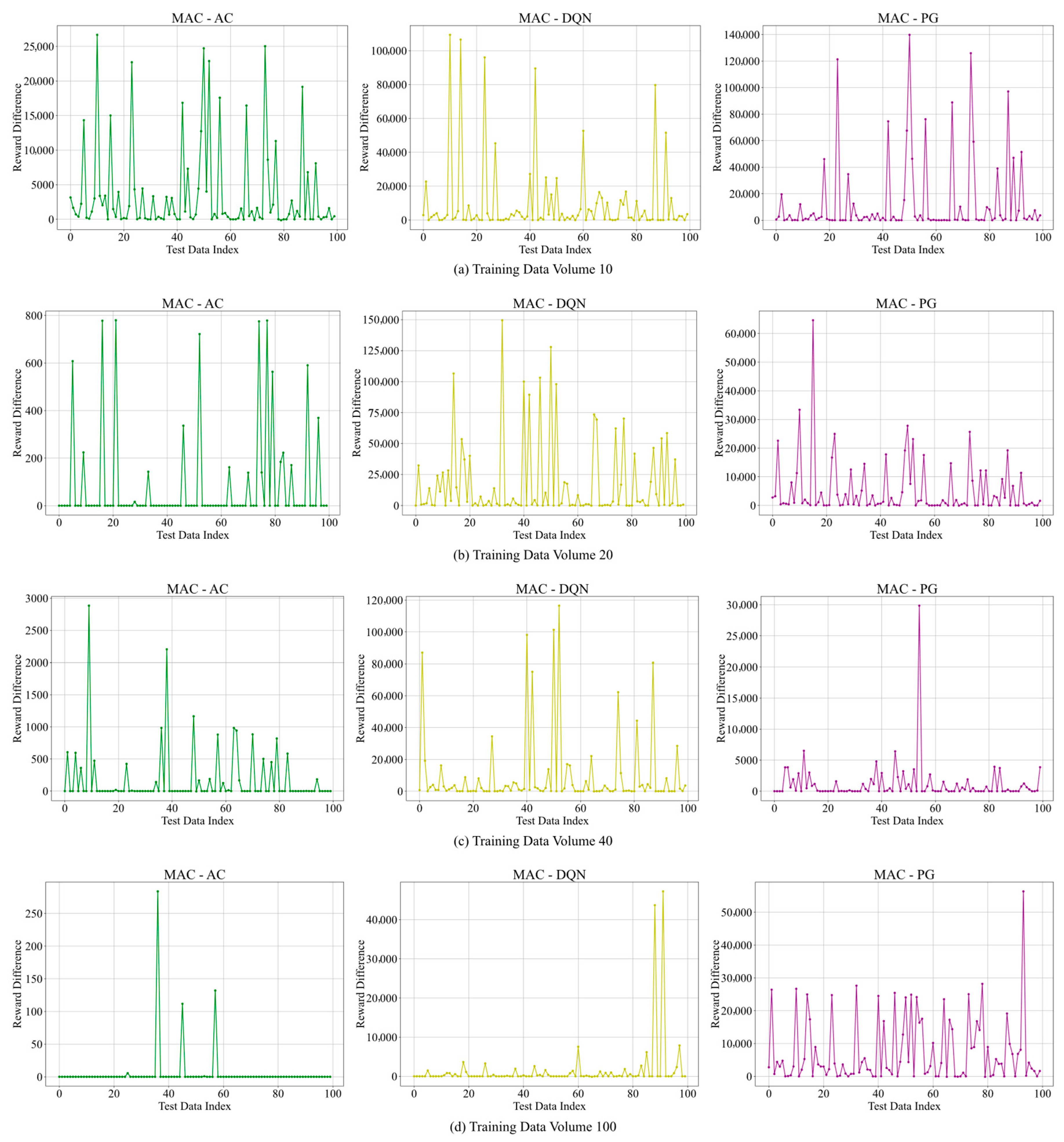
When training the model, different training data amounts are used to simulate different environments. The lack of training data corresponds to 10 and 20 data amounts, the medium amount of training data corresponds to 40 and 60, and the sufficient training data corresponds to 100 and 200. The following is the difference between the MAC algorithm and Actor–Critic, DQN, and PG when the amount of training data is 10, 20, 40, and 100, respectively. The green line represents the reward difference between MAC and Actor–Critic, the yellow line represents the reward difference between MAC and DQN, and the purple line represents the reward difference between MAC and PG.
As can be seen from Figure 4, the total task reward of the MAC algorithm is always no worse than that of the AC algorithm and DQN algorithm. The MAC algorithm demonstrates significant performance advantages over AC, DQN, and PG algorithms across varying training data volumes. When the training data volume is 10, the reward difference between MAC and AC shows intense fluctuations with peaks exceeding 25,000. The differences are even more pronounced when comparing MAC to DQN and PG, reaching 100,000 and 140,000, respectively, indicating MAC’s superior performance and stability in data-scarce environments. As the training data volume increases to 20, the fluctuation amplitude of reward differences begins to converge. The peak difference between MAC and AC decreases notably, though MAC maintains substantial advantages over DQN and PG, demonstrating improved stability with additional data. When the training data volume reaches 40, the peak difference between MAC and AC narrows to approximately 2500, showing converging performance. However, extreme peaks of 100,000 still occasionally appear in MAC-DQN comparisons, highlighting MAC’s stronger generalization capability in complex tasks. At the maximum data volume of 100, all algorithms show reduced fluctuation, with MAC-AC differences approaching zero while MAC maintains stable advantages over DQN and PG, confirming MAC’s robustness and convergence superiority across all data scales.
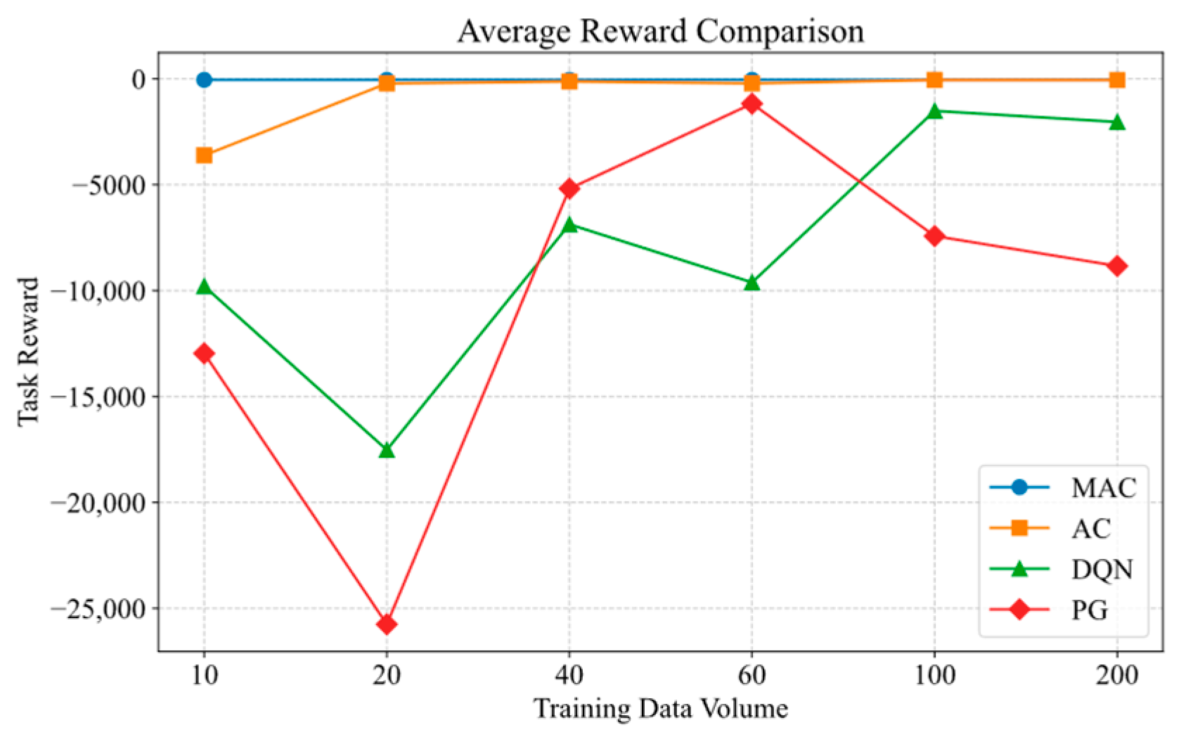
Figure 5 shows the comparison of average total reward values:
From the perspective of average reward value, MAC shows stable excellence and can still approach the optimal value in the case of extremely scarce training data, while both traditional AC and DQN need a long adaptation process, and DQN performs poorly in the case of extremely low training data. AC can also achieve the optimal value when the training data is sufficient, while the DQN algorithm evidently needs a larger amount of training data to achieve the optimal performance.
(3)
Comparison of Time Consumption
Figure 6 shows a comparison of the time consumption of algorithms with different amounts of training data. Due to the need for multiple optimizations of the inner and outer layers in the MAML framework, the computation is relatively complex. MAML requires training on multiple tasks, while traditional AC and PG algorithms only focus on a single task, resulting in a more complex and time-consuming training process for the MAC algorithm. Moreover, the MAC algorithm is slightly slower than traditional AC and PG algorithms, maintaining a gap of about 1 s compared to AC and PG algorithms. In contrast, the DQN algorithm has a significant disadvantage when dealing with large amounts of data, with MAC reducing the training time by 97.23% compared to DQN. This is mainly because the MAML framework effectively utilizes shared knowledge between tasks through training on multiple tasks, reducing the time required for each task to be trained separately. Meanwhile, due to the design of MAML meta tasks, the model can quickly achieve optimal strategies during the training process. It avoids the long exploration and adjustment in traditional algorithms [17].
(4)
Comparison of Balanced Performance Index
We define the calculation formula for BPI as follows:
B P I = 0.8 · R E R + 0.2 · T I R × 100 %
where R E R is the Reward Efficiency Ratio. In this experiment, we can derive the optimal reward value as B e s t   R e w a r d , and the reward values for the three methods at each training data size are A v e r a g e   R e w a r d . Thus, the calculation formula for R E R iscas follows:
R E R = B e s t   R e w a r d A v e r a g e   R e w a r d
T I R stands for Time Idle Rate, which indicates the proportion of idle time to the upper limit of runtime in whole minutes. Its calculation formula is as follows:
T I R = m a x T i m e T i m e C o m p a r s i o n m a x T i m e
Since “optimal decision-making” is the primary objective of the decision model, the improvement of time efficiency is secondary. However, the sacrifice of time performance is minimal, and increasing the weight of R E R can better demonstrate the superiority of the MAC algorithm under data scarcity. Therefore, we set the weight of R E R to 0.8 and the weight of T I R to 0.2.
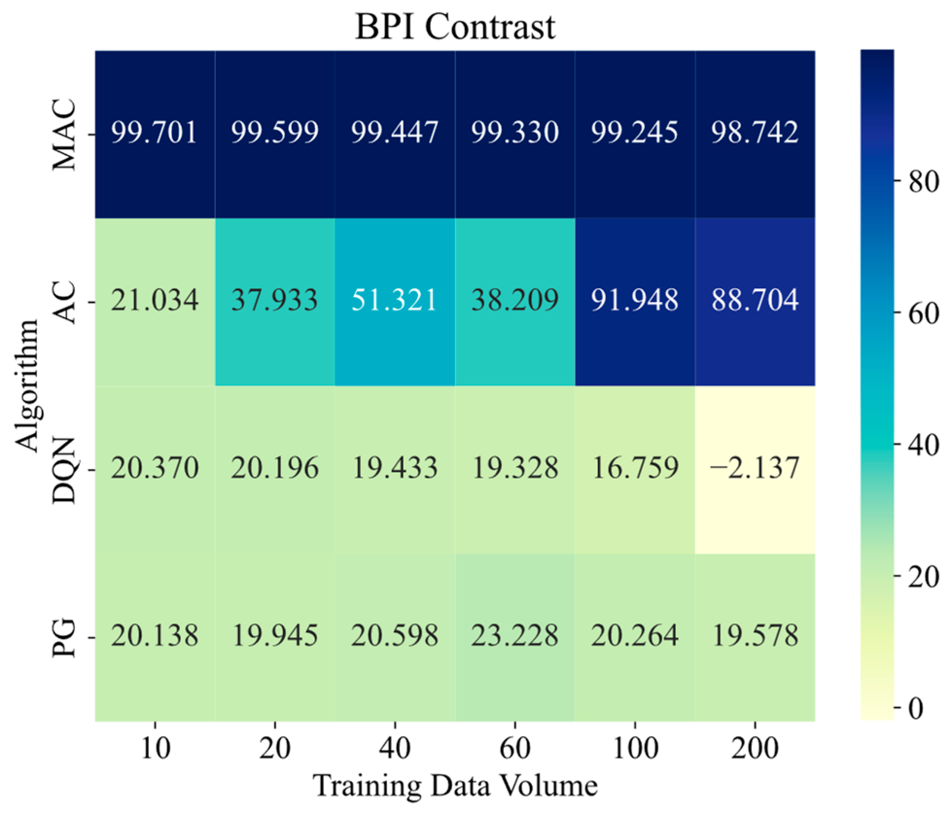
The BPI comparison chart visually displays the performance of each algorithm. Clearly, in scenarios with low training data, the MAC algorithm shows a significant performance advantage. With only 10 training data points, the BPI already reaches 99.701, indicating that it requires the least amount of data to achieve the optimal strategy.
As the amount of data increases, the traditional AC algorithm improves its performance due to the enhancement in the Reward Efficiency Ratio, ultimately coming close to that of the MAC algorithm. It appears that the AC algorithm needs more information to sharpen its predictions and boost its performance. On the other hand, the DQN algorithm tends to take a lot of time and depends heavily on training data. This can lead to poorer results, showing that it has a big appetite for data and does not handle low data situations very well. Although the time difference between the PG algorithm and the MAC algorithm is not significant, its performance on the test set is poor, resulting in a very low BPI performance.
The BPI for the three algorithms is normalized and presented in Figure 7.
(5)
Comparison of Algorithm BPI under Different Random Seed Conditions
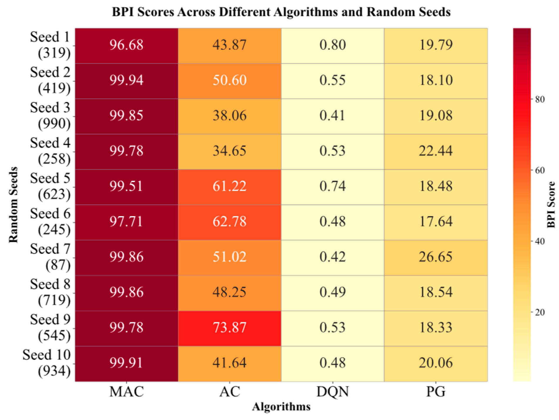
We repeated the algorithm comparison experiments under different random seeds and presented the results in Figure 8.
Results show BPI scores between 96.68 and 99.94, averaging close to 99 points, which indicates exceptional stability and superiority. In contrast, the AC algorithm exhibits considerable fluctuation in performance, with scores ranging from 34.65 to 73.87, and although it can achieve relatively good results under certain random seeds, its overall stability is notably insufficient. The DQN algorithm performs poorly under all testing conditions, with scores consistently below 1 point, suggesting fundamental adaptation issues with this algorithm in the current task environment. The PG algorithm shows relatively stable performance, with scores mostly concentrated between 17 and 27 points, which, while far inferior to the MAC algorithm, is considerably better than the DQN algorithm. Overall, the experimental results clearly demonstrate that the MAC algorithm not only significantly outperforms other algorithms in terms of average performance, but more importantly, its stability across different random seeds is exceptional, which holds important practical value in real-world applications [18].
(6)
Generalization experiments under different environmental conditions.
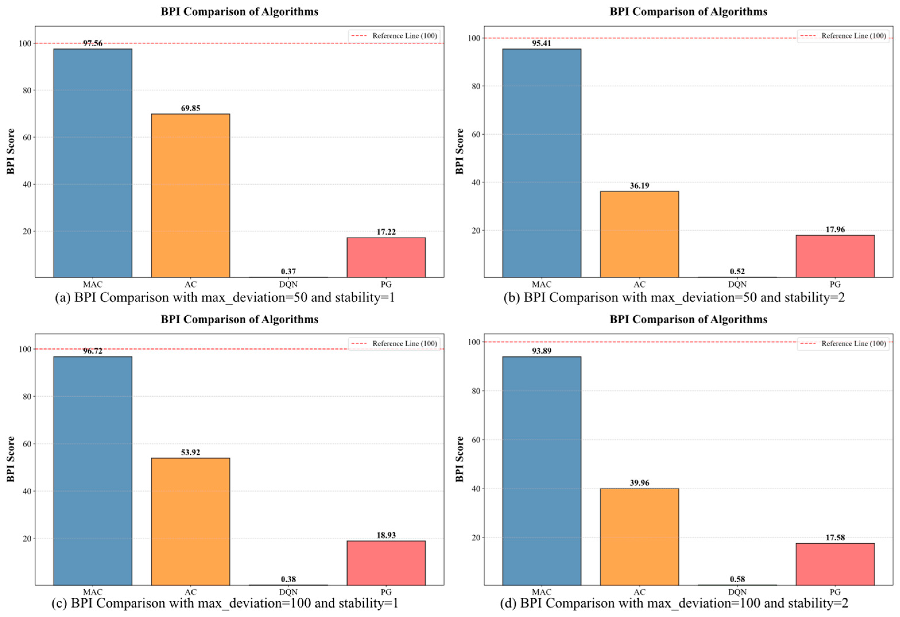
We repeated the algorithm comparison experiments under different environmental conditions, conducting generalization tests by adjusting the normal range size and maximum deviation range size, and presented the results in Figure 9.
Results show scores from 93.89 to 97.56, showcasing strong environmental adaptation capabilities. In contrast, the AC algorithm’s performance is significantly affected by changes in environmental parameters, with scores fluctuating from 36.19 to 69.85, particularly achieving its best performance under conditions with maximum deviation of 50 and stability parameter of 1, but showing notable performance degradation under other configurations. The DQN algorithm performs extremely poorly across all testing environments, with scores consistently below 1 point, indicating that this algorithm lacks basic adaptability to environmental changes. The PG algorithm exhibits relatively stable mid-level performance, with scores fluctuating slightly between 17.22 and 18.93, and although its absolute performance is limited, it at least maintains a certain level of consistency. Overall, this set of generalization test experiments fully validates that the MAC algorithm not only possesses excellent absolute performance, but, more importantly, demonstrates strong robustness when facing changes in different environmental parameters [19], making the MAC algorithm more reliable and practically valuable in real-world applications.

6. Experimental Results Analysis

6.1. Performance Superiority Under Data Scarcity

The most significant finding emerges from the algorithm’s performance under data-scarce conditions. With only 10 training samples, the MAC algorithm achieves a BPI score of 99.701, substantially outperforming traditional methods. The reward difference analysis reveals that MAC consistently outperforms AC by margins exceeding 25,000 points, while the gap with DQN and PG algorithms reaches 100,000 and 140,000 points, respectively, under minimal data conditions. This exceptional sample efficiency stems directly from the meta-learning architecture, which enables the model to leverage knowledge acquired from prior tasks. By learning an effective initialization or policy gradient update rule, MAC rapidly adapts to new tasks with minimal data, highlighting a fundamental advantage of meta-learning in low-data regimes [20].

6.2. Robustness Validation

The multi-seed experimental validation confirms the algorithm’s robustness across different initialization conditions. MAC maintains BPI scores between 96.68 and 99.94 across all tested random seeds, with an average approaching 99 points. This consistency contrasts sharply with the AC algorithm’s volatile performance, which fluctuates between 34.65 and 73.87 points depending on initialization conditions. The standard deviation of MAC’s performance across seeds is minimal, indicating reliable deployment potential in production environments. Such robustness is a hallmark of meta-learning approaches, which are designed to generalize across varying conditions through structured prior experience. The meta-training process allows MAC to avoid overfitting to specific random initializations, thereby producing more stable and reproducible outcomes—an essential feature for real-world applications [21].

6.3. Environmental Adaptability

The generalization experiments under varying environmental conditions provide crucial insights into the algorithm’s practical applicability. Across four different parameter configurations testing normal range and maximum deviation variations, MAC demonstrates exceptional environmental adaptability with BPI scores ranging from 93.89 to 97.56. The relatively narrow performance band indicates that the algorithm’s effectiveness remains largely independent of specific environmental parameters, a critical requirement for enterprise deployment where operational conditions may vary significantly [22]. This adaptability is enhanced by meta-learning, which trains the model on a distribution of tasks, thereby inoculating it against environmental shifts. The ability to maintain high performance across diverse settings underscores how meta-learning promotes generalizable policy learning, far surpassing the narrow adaptability of conventional algorithms.

6.4. Decision Quality Assessment

The comparative decision process analysis reveals MAC’s superior strategic selection capability. In all tested scenarios, MAC algorithms consistently guide system states back to normal intervals more rapidly than baseline methods. This behavior validates the meta-learning framework’s ability to identify optimal decision sequences efficiently, even when baseline algorithms eventually converge to similar solutions. The rapid convergence capability translates directly to reduced operational risk in real-world enterprise anomaly correction scenarios. The improved decision quality arises from meta-learning’s emphasis on learning high-level strategies rather than task-specific policies. By distilling broadly useful decision principles, MAC achieves more efficient and robust sequential decision-making—a key benefit in dynamic and time-sensitive environments.

7. Conclusions

Research on intelligent decision analysis holds significant implications, driving progress in technological fields like artificial intelligence and machine learning while demonstrating substantial practical value. However, existing intelligent decision analysis systems still exhibit certain shortcomings.
Within decision systems, the process is susceptible to negative influences such as decision-maker preferences, cognitive biases, and the rationality of decision quantification, potentially leading to irrational decisions and significant losses. To address this, this paper proposes an AHP-CRITIC weight quantification method, providing decision quantification that balances subjective and objective factors for effective decision-making. The AHP method constructs judgment matrices based on the decision-maker’s expertise and experience to determine the relative importance of different criteria and alternatives. Conversely, the CRITIC method focuses on utilizing inherent data characteristics, such as the coefficient of variation and conflict degree, to evaluate the importance of criteria or alternatives, enhancing the objectivity and scientific rigor of decisions.
Addressing limitations of Reinforcement Learning algorithms widely used in intelligent decision-making—namely, high data dependency and slow generalization—this paper proposes an Actor–Critic algorithm based on the MAML framework. The MAML-based Actor–Critic algorithm enables rapid adaptation to new tasks with minimal gradient updates, reducing training time and data requirements. Through meta-learning across multiple tasks, the model achieves superior generalization to unseen tasks, enhancing adaptability. The integration of these elements forms the intelligent decision analysis model proposed in this paper, combining the MAML framework with the Actor–Critic algorithm.
Comparative experiments validated the superior performance of the proposed MAML-based Actor–Critic decision analysis model. By comparing the total task reward values of different algorithms across varying training data volumes, the model’s advantage under low-data conditions was evident: its average total task reward consistently matched or exceeded that of the two baseline algorithms. Comparisons of time consumption across data volumes also demonstrated the model’s effective improvement in training speed. Utilizing the BPI metric we proposed, the experiment further verified the effectiveness of the AHP-CRITIC method and the Actor-Critic algorithm based on MAML in terms of rapid generalization and adaptability, particularly in scenarios where training data is scarce.
Despite the progress achieved, this study has limitations and suggests future research directions. For instance, the model was primarily tested within the designed simulated environment of enterprise indicator anomaly decision-making; future work could extend its application to more diverse environments. Moreover, while the MAML framework effectively enhances model generalization, its computational cost is relatively high. Finding ways to reduce computational resource consumption while maintaining performance remains a key focus for future research.
In conclusion, this research provides a viable pathway for the development of intelligent decision models and identifies directions for future investigation. With continuous technological advancement, we can reasonably expect intelligent decision models to play increasingly important roles across diverse domains, delivering greater value to human society.

Author Contributions

Conceptualization, X.Z., B.Z. and H.L.; methodology, X.Z.; software, X.Z.; validation, X.Z.; formal analysis, H.W.; investigation, Y.H.; resources, B.Z.; data curation, X.Z.; writing—original draft preparation, X.Z.; writing—review and editing, X.Z. and B.Z.; visualization, X.Z.; supervision, B.Z.; project administration, H.L.; funding acquisition, B.Z. All authors have read and agreed to the published version of the manuscript.

Funding

This research was funded by the Natural Science Foundation of Shaanxi Province, China (Grant No. 2021JM-344), the Independent Research Project of Shaanxi Provincial Key Laboratory of Network Computing and Security Technology (Grant No. NCST2021YB-05), and the Shaanxi Provincial Key R&D Program (Grant No. 2018ZDXM-GY-036). The APC was funded by the authors’ institution.

Conflicts of Interest

The authors declare no conflict of interest.

References

  1. Sutton, R.S.; Barto, A.G. Reinforcement Learning: An Introduction. IEEE Trans. Neural Netw. 1998, 9, 1054. [Google Scholar] [CrossRef]
  2. Konda, V.R.; Tsitsiklis, J.N. On Actor-Critic Algorithms. In Proceedings of the International Conference on Machine Learning, Los Angeles, CA, USA, 23–24 June 2003; Society for Industrial and Applied Mathematics: Washington, DC, USA, 2003; pp. 1008–1014. [Google Scholar]
  3. Mnih, V.; Badia, A.P.; Mirza, M.; Graves, A.; Lillicrap, T.; Harley, T.; Silver, D.; Kavukcuoglu, K. Asynchronous Methods for Deep Reinforcement Learning. In Proceedings of the 33rd International Conference on Machine Learning (ICML 2016), New York, NY, USA, 19–24 June 2016; ICML Press: New York, NY, USA, 2016; pp. 1928–1937. [Google Scholar]
  4. Mnih, V.; Kavukcuoglu, K.; Silver, D.; Rusu, A.A.; Veness, J.; Bellemare, M.G.; Graves, A.; Riedmiller, M.; Fidjeland, A.K.; Ostrovski, G.; et al. Human-Level Control through Deep Reinforcement Learning. Nature 2015, 518, 529–533. [Google Scholar] [CrossRef] [PubMed]
  5. Schulman, J.; Wolski, F.; Dhariwal, P.; Radford, A.; Klimov, O. Proximal Policy Optimization Algorithms. arXiv 2017, arXiv:1707.06347. Available online: https://arxiv.org/abs/1707.06347 (accessed on 16 July 2025). [CrossRef]
  6. Fujimoto, S.; Van Hoof, H.; Meger, D. Addressing Function Approximation Error in Actor-Critic Methods. arXiv 2018, arXiv:1802.09477. Available online: https://arxiv.org/abs/1802.09477 (accessed on 16 July 2025). [CrossRef]
  7. Jiang, S.; Zeng, Y.; Zhu, Y.; Pou, J.; Konstantinou, G. Stability-Oriented Multiobjective Control Design for Power Converters Assisted by Deep Reinforcement Learning. IEEE Trans. Power Electron. 2023, 38, 12394–12400. [Google Scholar] [CrossRef]
  8. Zeng, Y.; Jiang, S.; Konstantinou, G.; Pou, J.; Zou, G.; Zhang, X. Multi-Objective Controller Design for Grid-Following Converters with Easy Transfer Reinforcement Learning. IEEE Trans. Power Electron. 2025, 40, 6566–6577. [Google Scholar] [CrossRef]
  9. Finn, C.; Abbeel, P.; Levine, S. Model-Agnostic Meta-Learning for Fast Adaptation of Deep Networks. In Proceedings of the 34th International Conference on Machine Learning (ICML 2017), Sydney, Australia, 6–11 August 2017; ICML Press: Sydney, Australia, 2017; Volume 3, pp. 1126–1135. [Google Scholar]
  10. Chen, Y.Y.; Huo, J.; Ding, T.Y.; Gao, Y. A Survey of Meta Reinforcement Learning. Ruan Jian Xue Bao (J. Softw.) 2024, 35, 1618–1650. [Google Scholar] [CrossRef]
  11. Munikoti, S.; Natarajan, B.; Halappanavar, M. GraMeR: Graph Meta Reinforcement Learning for Multi-Objective Influence Maximization. J. Parallel Distrib. Comput. 2024, 192, 109–123. [Google Scholar] [CrossRef]
  12. Shi, Y.G.; Cao, Y.; Chen, Y.; Zhang, L. Meta Learning Based Residual Network for Industrial Production Quality Prediction with Limited Data. Sci. Rep. 2024, 14, 8122. [Google Scholar] [CrossRef] [PubMed]
  13. Zhang, L.; Li, D.; Xi, Y.; Jia, S. Reinforcement Learning with Actor-Critic for Knowledge Graph Reasoning. Sci. China Inf. Sci. 2020, 63, 223–225. [Google Scholar] [CrossRef]
  14. Mazouchi, M.; Nageshrao, S.; Modares, H. Conflict-Aware Safe Reinforcement Learning: A Meta-Cognitive Learning Framework. IEEE/CAA J. Autom. Sin. 2022, 9, 466–481. [Google Scholar] [CrossRef]
  15. Saaty, T.L. The Analytic Hierarchy Process; McGraw-Hill: New York, NY, USA, 2001. [Google Scholar]
  16. Diakoulaki, D.; Mavrotas, G.; Papayannakis, L. Determining Objective Weights in Multiple Criteria Problems: The CRITIC Method. Comput. Oper. Res. 1995, 22, 763–770. [Google Scholar] [CrossRef]
  17. Zhang, H.G.; Liu, C.; Wang, J.; Ma, L.; Koniusz, P.; Torr, P.H.; Yang, L. Saliency-Guided Meta-Hallucinator for Few-Shot Learning. Sci. China Inf. Sci. 2024, 67, 132101. [Google Scholar] [CrossRef]
  18. Zhou, S.; Cheng, Y.; Lei, X.; Duan, H. Multi-Agent Few-Shot Meta Reinforcement Learning for Trajectory Design and Channel Selection in UAV-Assisted Networks. In Proceedings of the IEEE International Conference on Communications (ICC 2022), Seoul, Republic of Korea, 16–20 May 2022; IEEE Press: Shanghai, China, 2022; pp. 166–176. [Google Scholar]
  19. Guo, S.; Du, Y.; Liu, L. A Meta Reinforcement Learning Approach for SFC Placement in Dynamic IoT-MEC Networks. Appl. Sci. 2023, 13, 9960. [Google Scholar] [CrossRef]
  20. Zhao, T.T.; Li, G.; Song, Y.; Wang, Y.; Chen, Y.; Yang, J. A Multi-Scenario Text Generation Method Based on Meta Reinforcement Learning. Pattern Recognit. Lett. 2023, 165, 47–54. [Google Scholar] [CrossRef]
  21. Wei, Z.C.; Zhao, Y.; Lyu, Z.; Yuan, X.; Zhang, Y.; Feng, L. Cooperative Caching Algorithm for Mobile Edge Networks Based on Multi-Agent Meta Reinforcement Learning. Comput. Netw. 2024, 242, 110247. [Google Scholar] [CrossRef]
  22. Xi, X.; Li, J.; Long, Y.; Wu, W. MRLCC: An Adaptive Cloud Task Scheduling Method Based on Meta Reinforcement Learning. J. Cloud Comput. 2023, 12, 75. [Google Scholar] [CrossRef]
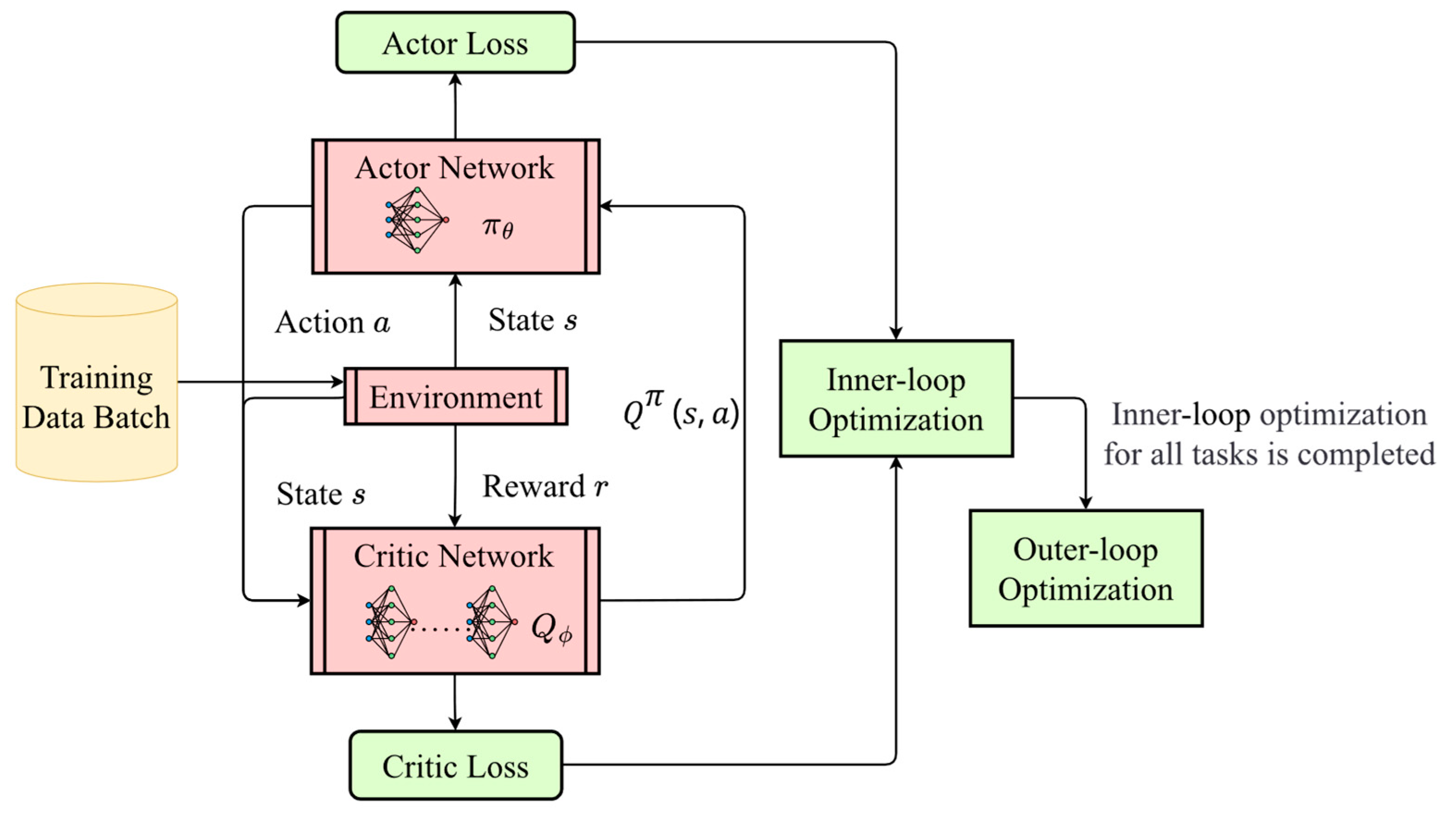
Figure 1. Training flowchart of the Actor–Critic algorithm based on the MAML framework.
Ai 06 00231 g001
Figure 2. Flowchart of the AHP-CRITIC weight calculation method.
Ai 06 00231 g002
Figure 3. Decision process diagram for part of test tasks.
Ai 06 00231 g003
Figure 4. Performance of different algorithms under various training data volumes.
Ai 06 00231 g004
Figure 5. Comparison of average total reward values.
Ai 06 00231 g005
Figure 6. Comparison of time consumption.
Ai 06 00231 g006
Figure 7. BPI contrast.
Ai 06 00231 g007
Figure 8. BPI scores across different algorithms and random seeds.
Ai 06 00231 g008
Figure 9. Comparison of BPI under different environmental conditions.
Ai 06 00231 g009
Table 1. Partial view of the strategy rating table.
Abnormal Interval (Percentage)Strategy GroupParticipant AConstraint CriteriaRating (0–9)
10~201Strategy aa1Criteria 12
Criteria 24
Criteria 34
2Strategy aa2Criteria 17
Criteria 22
Criteria 31
3Strategy aa3Criteria 16
Criteria 22
Criteria 32
Table 2. Strategy group setup.
Abnormal IntervalStrategy Group 1
(Strategy Name, Benefit Value)
Strategy Group 2
(Strategy Name, Benefit Value)
Strategy Group 3
(Strategy Name, Benefit Value)
[−50%, 20%)“A1”, 35“A2”, 25“A3”, 15
[−20%, 10%)“B1”, 15“B2”, 11“B3”, 8
[−10%, −5%)“C1”, 8“C2”, 6“C3”, 4
[−5%, 0%)“D1”, 1“D2”, 0.5“D3”, 0.2
[0%, 5%)“E1”, −1“E2”, −0.5“E3”, −0.2
[5%, 10%)“F1”, −8“F2”, −6“F3”, −4
[10%, 20%)“G1”, −15“G2”, −11“G3”, −8
[20%, 50%)“H1”, −35“H2”, −25“H3”, −15
Table 3. Network parameter settings.
ParameterValue
MAML inner learning rate0.01
MAML outer learning rate0.01
Meta-task batch size5
the learning rate of the Actor and Critic networks0.001
Discount factor0.98
Number of hidden layers in the Actor network3
Number of hidden layers in the Critic network3
Number of neurons in each hidden layer of
the Actor network and Critic network
128, 256, 128
Activation function of the Actor networkSoftmax, ReLU
Activation function of the Critic networkReLU
OptimizerAdam
Learning rate schedulerStepLR
Learning rate decay step size200
Learning rate decay factor0.5
AHP-CRITIC weight coefficient0.6
Disclaimer/Publisher’s Note: The statements, opinions and data contained in all publications are solely those of the individual author(s) and contributor(s) and not of MDPI and/or the editor(s). MDPI and/or the editor(s) disclaim responsibility for any injury to people or property resulting from any ideas, methods, instructions or products referred to in the content.