Knee Osteoarthritis Detection and Classification Using Autoencoders and Extreme Learning Machines

Abstract

Background/Objectives: Knee osteoarthritis (KOA) is a prevalent disorder affecting both older adults and younger individuals, leading to compromised joint function and mobility. Early and accurate detection is critical for effective intervention, as treatment options become increasingly limited as the disease progresses. Traditional diagnostic methods rely heavily on the expertise of physicians and are susceptible to errors. The demand for utilizing deep learning models in order to automate and improve the accuracy of KOA image classification has been increasing. In this research, a unique deep learning model is presented that employs autoencoders as the primary mechanism for feature extraction, providing a robust solution for KOA classification. Methods: The proposed model differentiates between KOA-positive and KOA-negative images and categorizes the disease into its primary severity levels. Levels of severity range from “healthy knees” (0) to “severe KOA” (4). Symptoms range from typical joint structures to significant joint damage, such as bone spur growth, joint space narrowing, and bone deformation. Two experiments were conducted using different datasets to validate the efficacy of the proposed model. Results: The first experiment used the autoencoder for feature extraction and classification, which reported an accuracy of 96.68%. Another experiment using autoencoders for feature extraction and Extreme Learning Machines for actual classification resulted in an even higher accuracy value of 98.6%. To test the generalizability of the Knee-DNS system, we utilized the Butterfly iQ+ IoT device for image acquisition and Google Colab’s cloud computing services for data processing. Conclusions: This work represents a pioneering application of autoencoder-based deep learning models in the domain of KOA classification, achieving remarkable accuracy and robustness.

1. Introduction

Knee osteoarthritis (KOA) is a common disease in elderly people due to the degeneration of the articular cartilage between knee joints. Research papers show that KOA will affect approximately 130 million people globally by 2050 [1]. This disease has different symptoms, such as joint noises, pain, stiffness, and swelling. According to these symptoms, pain is the most apparent symptom for the patient. 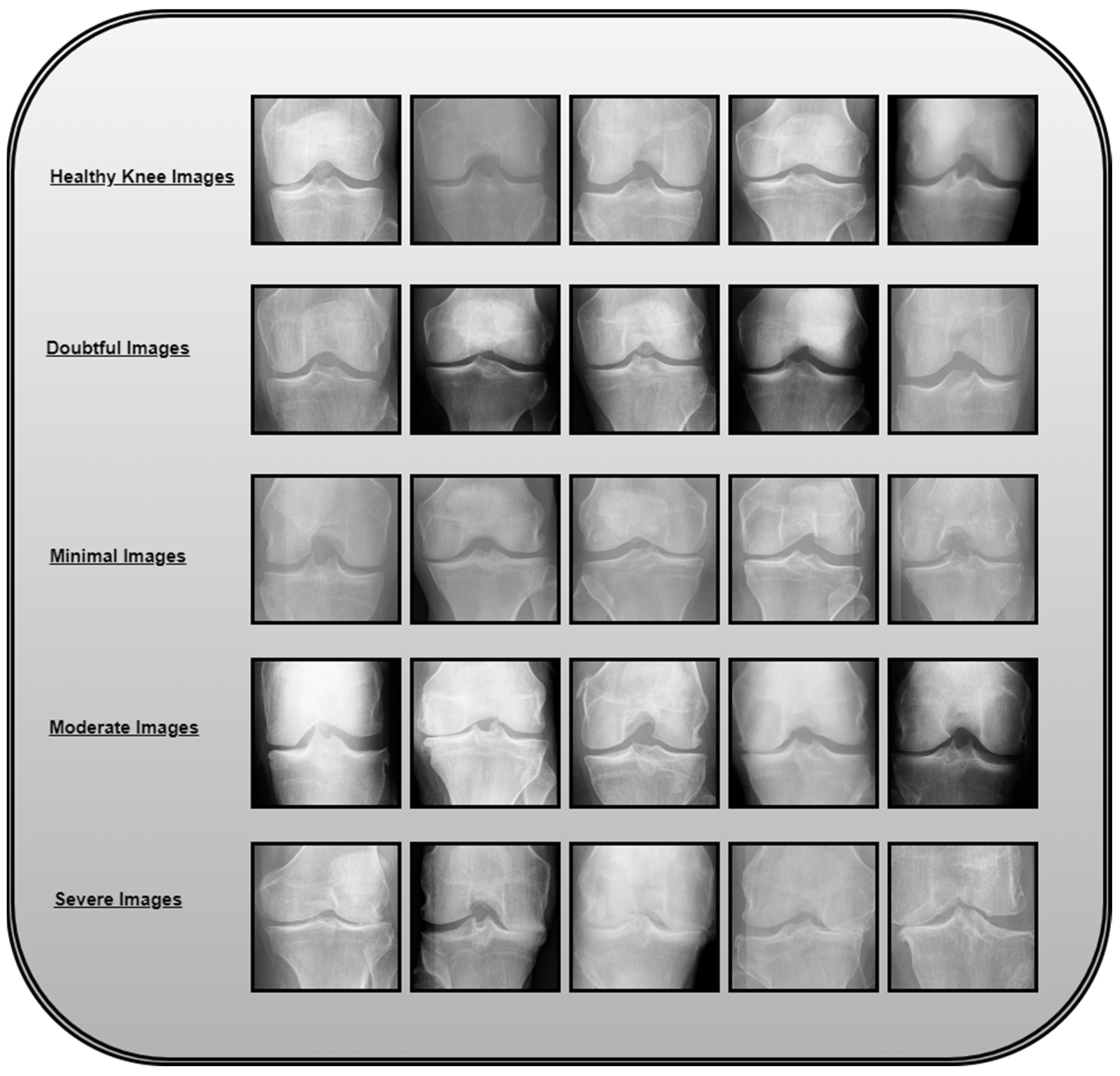This symptom drives patients to seek medical treatment [2]. Ultimately, the disease can cause loss of knee function in severe cases. Physicians can examine the joint and classify the disease severity according to the Kellgren–Lawrence (KL) grading system [3]. In 1961, the World Health Organization (WHO) accepted this system as a standard. The system classifies disease severity according to five grades of disease progression: 0 (healthy), 1 (doubtful), 2 (minimal), 3 (moderate), and 4 (severe). The main problem in diagnosing such a disease is the minimal difference between levels 0 and 1. This means the disease is complex for physicians to classify at early stages. This could result in the progression of the disease when undiagnosed by physicians. Also, the treatment options for such a disease decrease with the progression of the disease. At present, there are traditional examination methods for KOA. These methods depend on an expert’s imaging examination. This requires images of high quality and high-cost fees, hence the role of deep learning models for effectively diagnosing the disease at early stages.

Early diagnosis of such a disease can assist in treating the disease and reducing its progression. Many deep learning techniques are applied in medicine in current research, particularly for disease diagnosis. These DL models help build automatic systems for different disease classifications. In [4], an automatic classification system for acute lymphoblastic leukemia (ALL) is introduced. The proposed system uses a convolutional neural network with three convolutional layers for disease classification. First, the proposed CNN is trained on the labeled dataset; hence, the CNN learns the salient features of each class. Later, the proposed model is compared to three different deep learning networks: VGG-16, DenseNet, and Xception. The results show an improved performance of the constructed network, achieving an accuracy of 97%. In [5], a novel deep model for the diagnosis of pancreatic disease or chronic pancreatitis is developed. The novel deep learning model is called PANet. The model combines a pre-trained CNN, multi-scale feature modules, and attention mechanisms to achieve accuracies up to 95%. In [6], the authors develop a novel deep learning model to predict time to diabetic retinopathy progression within 5 years. The developed model is able to achieve high accuracies. In [7], the authors present a new Dual self-supervised Multi-operator transformation network, abbreviated as DSMT-Net, to improve multi-source EUS diagnosis. Accordingly, the new model constructs a multi-operator transformation mechanism to normalize region-of-interest extraction in EUS images and eliminate redundant pixels. In [8], a transformer-based deep learning model is proposed for image anomaly detection. The system achieves high accuracies. In [9], deep learning models are proposed to classify lung diseases from lung images. Three deep learning networks (VGG16, ResNet-50, and InceptionV3) are fine-tuned on a lung disease dataset. These models were previously trained using the ImageNet dataset. In the work, they are fine-tuned on lung images. This is called transfer learning. In the work, a pipeline is created for the application. The pipeline consists of a segmentation algorithm to segment chest images. The next step of the pipeline is the classification algorithm. The proposed result shows that pre-trained models, along with simple classifiers, are competent enough to (shallow neural networks) produce results comparable to those of complex systems. Figure 1 illustrates the knee osteoarthritis image categorization based on severity levels. 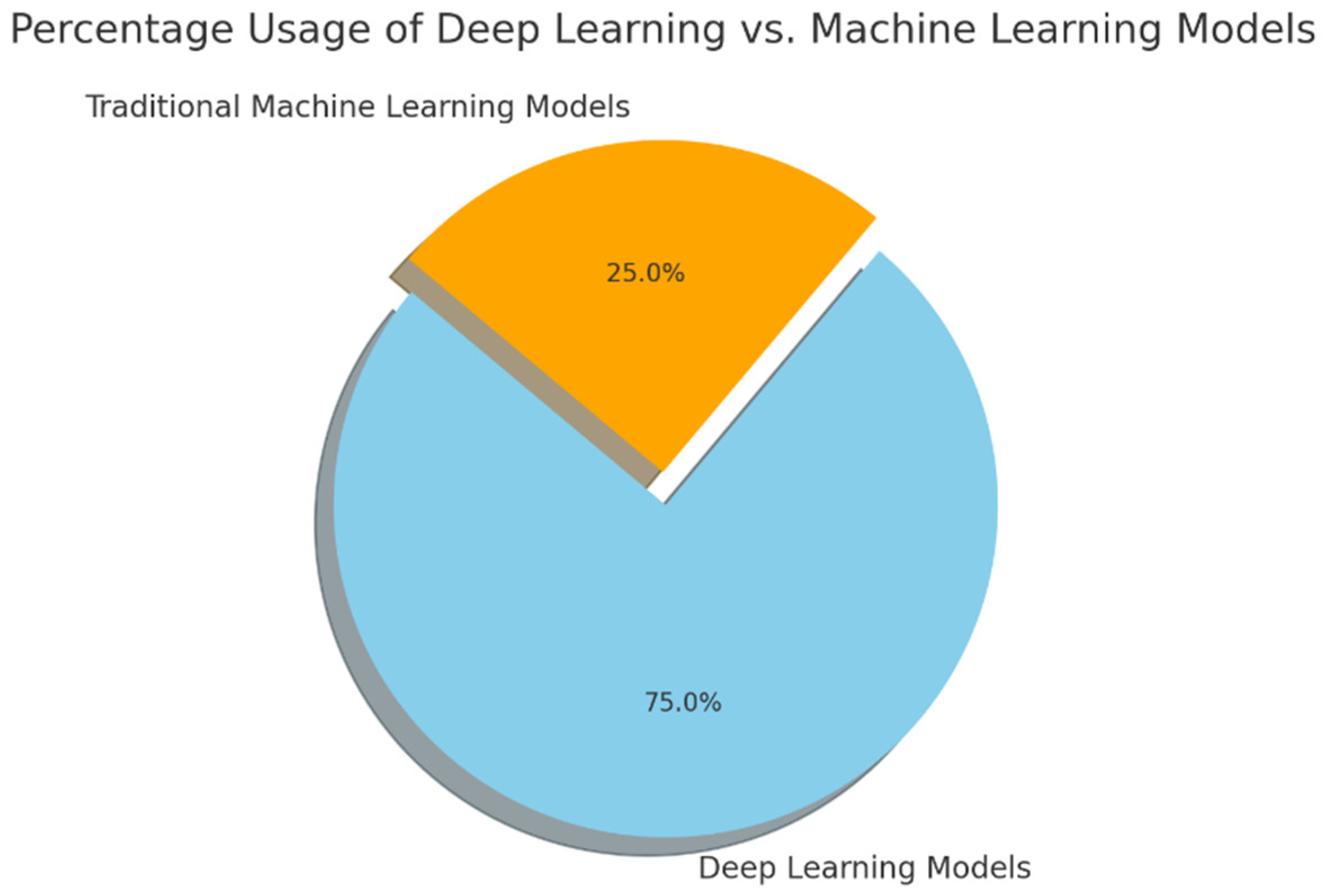Figure 2 illustrates the distribution of machine learning and deep learning techniques used in knee osteoarthritis detection and classification.

Table 1. Knee osteoarthritis disease findings by severity level.

Severity Level	Condition	Description
0	Healthy Knee Images	These images show no signs of joint damage or abnormalities. The knee structure appears normal with clear, well-defined bone contours and a healthy amount of joint space.
1	Doubtful Images	These images might show very slight or questionable signs of joint damage. It is often unclear whether any abnormalities are present, and diagnosis might require further investigation.
2	Minimal Images	These images reveal minimal signs of joint damage, such as slight bone spur growth, but still maintain a good amount of joint space with no significant erosion.
3	Moderate Images	These images show moderate joint damage. This may include definite bone spur growth, definite narrowing of joint space, and possibly the beginning of bone deformation.
4	Severe Images	These images display severe joint damage. Characteristics include large bone spur growth, significant joint space narrowing, severe bone deformation, and potentially bone-on-bone contact with minimal to no joint space left.

is a record of clinical findings about disorders of knee osteoarthritis.

1.1. Research Contribution

This work introduces the following contributions to KOA problem classification:

(1)

We propose an end-to-end deep learning architecture that uniquely integrates autoencoders for feature extraction with Extreme Learning Machines (ELMs) for classification. This combination has not been previously applied in the KOA classification literature to the best of our knowledge, marking a significant advancement in medical image analysis.

(2)

Two experimental setups validate the effectiveness of the proposed approach. In the first, autoencoders are employed for both feature extraction and classification, achieving a strong performance with 96.68% accuracy. The second setup leverages autoencoders for feature extraction while employing ELMs for classification, resulting in a superior 98.6% accuracy and demonstrating the potency of the hybrid method.

(3)

This study employs GAN-based data augmentation to synthetically balance the KOA dataset, enhancing minority class representation and improving model generalization. The integration of GANs led to a significant accuracy boost, particularly in underrepresented severity levels.

(4)

This study is the first to apply Grad-CAM for interpretability in knee osteoarthritis classification, providing visual explanations that highlight disease-relevant regions in X-ray images. This enhances the model’s transparency and supports clinical trust in AI-based KOA diagnosis.

(5)

The Knee-DNS system has high accuracy and reliability in classifying knee osteoarthritis across different severity levels, utilizing the Butterfly iQ+ IoT device for image acquisition and Google Colab’s cloud computing services for data processing, as evidenced by the results.

In the state-of-the-art comparison section, a proper comparison of the proposed work with other work in the literature ensures the better working of the proposed model. The superior performance can be demonstrated by its higher accuracy compared to other work in the literature.

1.2. Paper Organization

The remaining portion of this paper is organized as follows: Section 2 proposes related work through a literature survey. Section 3 describes the background knowledge for this work. Section 4 presents an introduction to the methodology of our proposed model. Section 5 presents the different experiments that were conducted using the proposed model. Section 6 discusses the results, and Section 7 discusses the conclusion of this paper.

2. Literature Survey

Over the last few years, numerous researchers have studied the issue of KOA classification using deep learning models. In this work, we present a review of the most up-to-date and relevant papers related to the topic. Feature extraction techniques are employed in [10] for image preprocessing before performing deep learning classification. Histogram of oriented gradients HOG and LDA, as well as min-max scaling, are the new feature extraction techniques employed. Six ML classifiers are employed and tested in the course of the study concerning the task of classifying KOA. These include the K-nearest neighbors classifier, Support Vector Machine, Gaussian Naive Bayes, Decision Tree, Random Forest, and XgBoost.

The research also entails investigating the ensemble modeling of these models. Based on the findings, the ensemble models are shown to improve accuracy and reduce the overfitting risk. The XgBoost classifier and ensemble model have the highest accuracy of 98.9% in distinguishing unhealthy from healthy knees.

In [11], six different pre-trained deep neural networks are proposed for the KOA classification method. These six models are VGG16, VGG19, ResNet101, MobileNetV2, InceptionResNetV2, and DensenNet121. The pre-trained models are fine-tuned on images obtained from the Osteoarthritis Initiative (OAI) dataset. The proposed work performs two types of classifications. First, binary classification is performed to check the presence or absence of KOA. The second classification is performed to find the severity of the disease in a three-class classification. In [12], transfer learning and pre-trained CNN models, like AlexNet and ResNet-50, are proposed. The developed system is evaluated using experimental testing. In the work, the proposed methodology uses Faster RCNN and Modified ResNet for region of interest extraction. The next step is to apply AlexNet to classify images. The results indicate the better performance of the proposed model. The proposed model is 98.5% accurate in knee joint detection and 98.90 accurate in classification.

In [13], a new model combining an object detection model (YOLO) with a visual transformer is proposed for the KOA classification problem. The segmentation model has an accuracy of 95.57% when trained on 200 annotated images from a large dataset containing more than 4500 samples. The suggested model enhances precision by 2.5% compared to conventional CNN architectures. In [14], the DenseNet169 deep learning model is proposed to solve the problem of KOA classification. The deep learning model is fine-tuned to achieve high performance. Grad-CAM is proposed for enhancing image quality. The proposed pipeline combines both Grad-CAM and deep learning models to increase the efficiency of the classification model. The model proposed can also be employed to classify the severity of KOA based on the multi-classification model. Artifact removal, resizing, contrast processing, and normalization are the first steps in the work. The proposed model is tested and compared with other similar work in the literature. It is also tested in multi-classification and binary classification. The DenseNet169 achieves 95.93% accuracy in multi-classification and 93.78% accuracy in binary classification.

In [15], different deep learning models are trained using a dataset of 8260 X-ray knee images from the Osteoarthritis Initiative open dataset. Each model is trained using the most suitable image size for the model. The trained models are used to build an ensemble of models. The proposed ensemble has better stability than single models and can achieve higher accuracy. The proposed ensemble network shows the best performance, achieving an accuracy of 76.93%. The results show that the proposed ensemble performs better than the available techniques in the literature. Further analysis shows that the proposed ensemble focuses on the joint space around the knee to extract the needed features for classification of the diseases. This proves the importance of the proposed model. In [16], the authors use transfer learning and fine-tuned deep learning models (ResNet-34, VGG-19, DenseNet-121, and DenseNet-161). The authors combine the models in an ensemble to improve the model’s accuracy and generalization. The proposed method shows promising results, achieving 98% accuracy. The proposed method outperforms state-of-the-art automated methods.

In [17], a novel Gaussian Aquila optimizer-based dual convolutional neural network model is proposed that identifies and grades osteoarthritis with the help of images of the knee joint. The work invents a novel dual convolutional neural network, which can balance the convolutional layers in each convolutional model. The newly developed Gaussian Aquila optimizer is used to optimize the weights and bias parameters of the new proposed DCNN. The proposed novel GAO-DCNN model achieves high performance. The proposed model is able to achieve an accuracy of 98.77% for abnormal knee joint images. In [18], an automatic deep learning model of osteoarthritis classification according to Kellgren–Lawrence in adult knee images is proposed. In the work, the main purpose is to determine if AI can classify the severity of knee OA using complete images of the knee without removing visual disturbances, such as implants. The authors of the work select 6103 radiographic exams from Danderyd University from 2002 to 2016. The images are manually categorized according to the Kellgren and Lawrence grading scale (KL). The photos are then used to train a ResNet architecture. The results show an average AUC of more than 0.95, indicating remarkable performance.

In [19], a hybrid feature extraction algorithm that combines Darknet53, Histogram of directional gradients (HOG), and Local Binary Model (LBP) methods for feature extraction is proposed. The work proposes a neighborhood component analysis (NCA) for feature selection. The proposed work is tested on a dataset containing 1650 knee joint images that are divided into five classes: normal, doubtful, mild, moderate, and severe. The proposed work compares the proposed model with eight convolutional neural network models. The developed model achieves higher accuracy than the other compared models.

In [20], a DenseNet201 deep learning network is proposed for detecting and grading knee osteoarthritis diseases. The paper compares the classification accuracy of the model and radiologists in detecting osteoarthritis in knee joints. The proposed model and radiologists are compared based on accuracy and statistical (Wilcoxon statistical test) testing. The results report that the proposed methodology shows the superior performance of the proposed Dl model. DenseNet201 is able to achieve 91.84% accuracy. The statistical testing proves no difference between classification results using DenseNet201 and radiologists’ opinions. The study concludes that DenseNet201 applies to the diagnosis of knee osteoarthritis and advises that radiologists verify diagnostic decisions. A summary of these techniques is presented in

Table 2. Overview of classification techniques based on deep learning.

Ref No.	Year	Methodology	Results
[10]	2024	▪ Oriented gradients histogram with Linear Discriminant Analysis and min-max scaling is performed. ▪ Six ML classifiers are tested and compared for the KOA classification problem.	98.9%
[11]	2023	▪ It proposes six different pre-trained deep neural networks, which include VGG16 and VGG19 models, ResNet101, MobileNetV2, InceptionResNetV2, and DensenNet121, to classify the KOA.	It allowed for the detection of the knee joint with an accuracy of 98.516%, giving an overall classification accuracy of 98.90%.
[12]	2022	▪ Two models are tested (AlexNet and ResNet-50).	Accuracy: 98.516%.
[13]	2021	▪ Object detection model combined with a visual transformer: YOLO.	The proposed model outperformed traditional CNN architectures in terms of accuracy by 2.5%.
[14]	2023	▪ Grad-CAM for image enhancement. ▪ DenseNet169 deep learning model for classification.	DenseNet169 achieved 95.93% accuracy in multi-classification and 93.78% accuracy for binary classification.
[15]	2023	▪ Different deep learning models are trained, and an ensemble model is created from these models.	Among the compared models, the proposed ensemble network attained the best performance with 76.93% accuracy.
[16]		▪ The deep learning models are ResNet-34, VGG-19, DenseNet-121 and DenseNet-161. ▪ Ensemble.	Ensemble achieved 98% accuracy
[17]	2024	▪ Novel Gaussian optimizer along with a newly invented DCNN.	98.25%
[18]	2021	▪ Convolutional neural network.	The results showed an average AUC of more than 0.95, indicating remarkable performance.
[19]	2024	▪ In the study, the proposed hybrid feature extraction method uses Darknet53, Histogram of directional gradients (HOG), and Local Binary Model (LBP) methods.	The developed model achieved higher accuracy than the other compared models.
[20]	2023	▪ DenseNet201.	DenseNet201 was able to achieve 91.84% accuracy.

, showcasing the diverse approaches and their outcomes.

Based on the critical analysis of the existing literature, several recurring limitations have been identified across prior studies. These include the reliance on computationally intensive architectures unsuitable for real-time or IoT-based deployment, insufficient handling of class imbalance in KOA datasets, the lack of feature-level explainability, such as Grad-CAM, limited exploration of hybrid lightweight models, and inadequate validation using clinical-grade imaging devices. Moreover, few studies have integrated generative data augmentation to improve minority class performance or leveraged autoencoders for efficient feature extraction. To address these gaps, the proposed Knee-DNS system introduces a novel, lightweight, and interpretable deep learning architecture that combines autoencoders with Extreme Learning Machines (ELMs), integrates GAN-based augmentation to handle data imbalance, and employs Grad-CAM for visual interpretability. Additionally, the system is validated using IoT-enabled ultrasound imaging, highlighting its potential for scalable, real-world clinical applications.

3. Background

3.1. Autoencoder

Autoencoders are deep learning models that take an input and transform it into another domain. They are versatile, finding applications in construction and various other fields [21]. Unlike traditional neural networks, autoencoders do not require a labeled dataset for training, making them an unsupervised learning model. They can learn an encoding function that transforms data input into a coded representation, which can then be used to generate the input by a decoding function. This unique ability makes autoencoders a promising tool for compression applications. Autoencoders were used in different research articles to enhance the performance of deep learning models. In [22], autoencoders are introduced to enhance video anomaly detection deep learning algorithms. The proposed framework is called the deep multiplicative attention-based autoencoder, and it is used to detect anomalies in video sequences. The developed system introduces an improved runtime for detecting anomalies in video sequences. In this context, we propose autoencoders as feature extraction models, demonstrating their potential in detecting attacks on web applications [23]. Figure 3 provides a visual representation of autoencoders.

3.2. Extreme Learning Machines (ELMs)

Extreme Learning Machines (ELMs) are feedforward neural networks known for their rapid training times and exceptional generalization performance. The core concept behind ELMs lies in their unique training process, where the input weights and biases are randomly initialized and remain fixed, eliminating the need for iterative adjustment. This simplification is central to ELMs efficiency. The training process involves only the calculation of output weights, which connect hidden nodes to the output layer. Moore–Penrose pseudoinverse of the hidden layer output matrix is employed to obtain these weights. It is an explicit way of solving the linear system of target values and the hidden layer outputs, as in the least squares solution. ELMs can be employed for classification and regression. The nonlinear activation function, for example, the sigmoid or hyperbolic tangent, changes the input features into the hidden layer feature space for classification. This ensures that the model can find complex patterns in the data. After training, predictions are made by applying the same transformation to new data and using the trained output weights to produce the final output, which can be adjusted via a threshold or decision function for classification tasks. Depending on the application, standard metrics, like accuracy, precision, and recall, can be used to judge the performance of ELMs even further. This is a simple but effective way to solve a wide range of predictive modeling problems [24]. Figure 4 shows the main architecture of ELMs.

4. Proposed Methodology

4.1. Dataset Acquisition

In this experiment, we ran the proposed model on a widely used dataset [25]. This dataset consists of 9786 X-ray images for knee joint detection and grading. The grading of this dataset can be described by the following points:

• Grade 0: Healthy knee image.
• Grade 1 (Doubtful): Questionable joint space narrowing with questionable osteophytic lipping.
• Grade 2 (Minimal): Definite osteophytes with possible narrowing of the joint space.
• Grade 3 (Moderate): Multiple osteophytes with definite joint space narrowing and mild sclerosis.
• Grade 4 (Severe): Large osteophytes, marked narrowing of joints, and severe sclerosis.

Table 3. Dataset representation.

Grade	Severity	Train	Validation (10%)	Testing (20%)	Auto-Testing
0	Healthy	2286	328	639	604
1	Doubtful	1046	153	296	275
2	Minimal	1516	212	447	403
3	Moderate	757	106	223	200
4	Severe	173	27	51	44
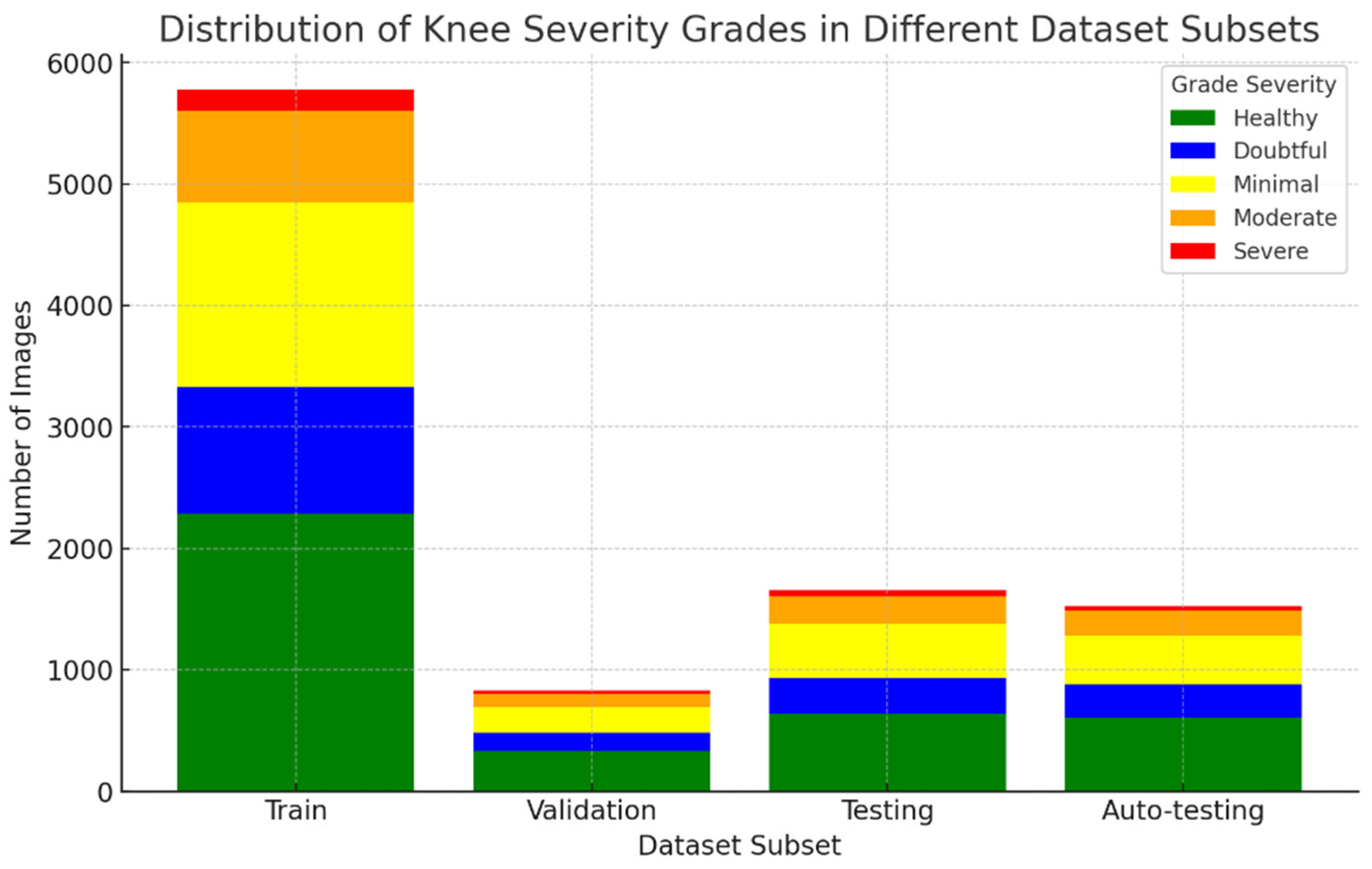
	Total	5778	826	1656	1526

shows the distribution of these dataset images into training, validation, testing, and auto-testing, as shown in Figure 5.

4.2. Data Preprocessing

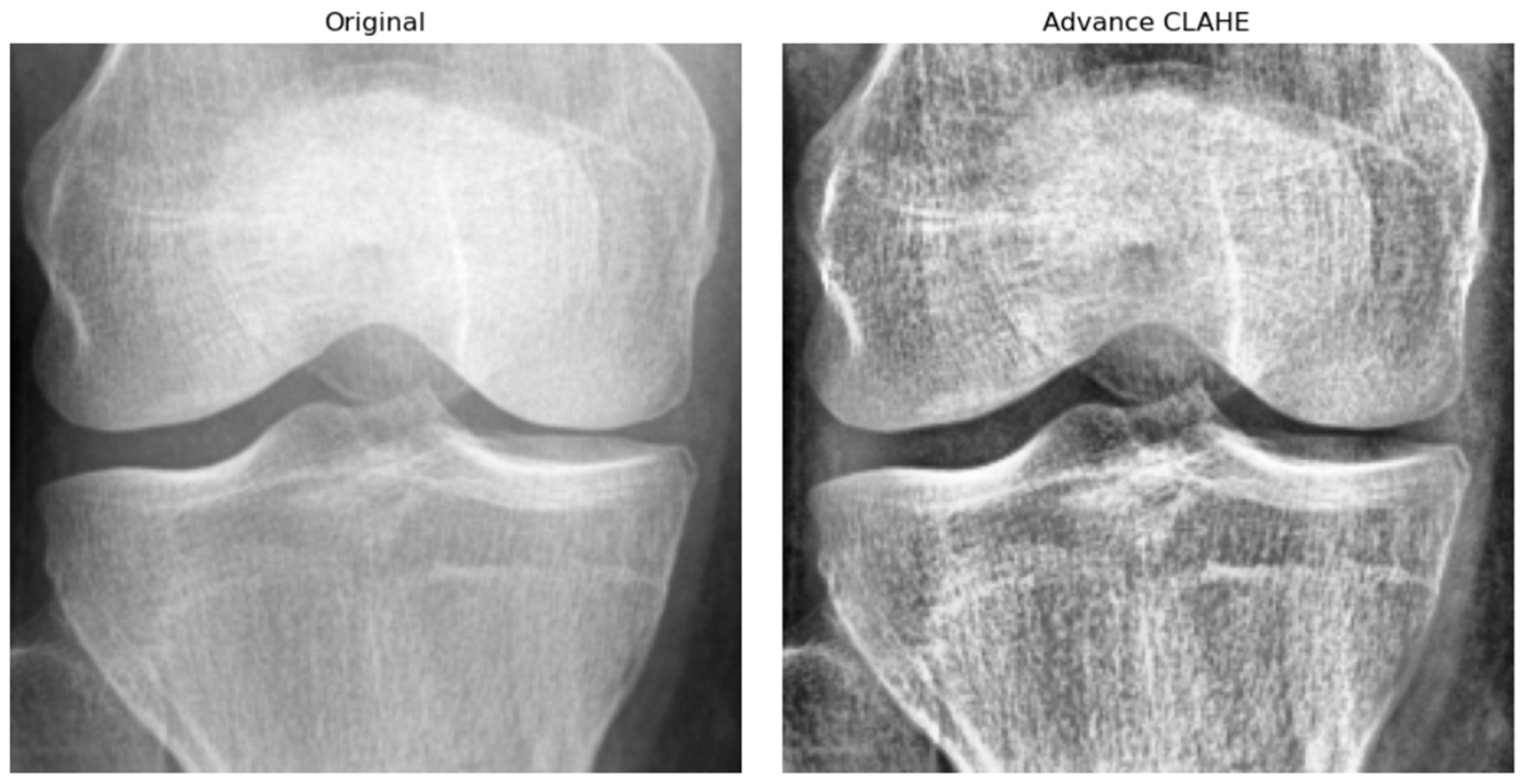
Prior to training the Knee-DNS model, a series of data preprocessing steps were applied to enhance the quality and uniformity of the X-ray images. First, all the images were resized to a fixed resolution of 700 × 600 pixels to standardize input dimensions and reduce computational complexity. Subsequently, advanced contrast-limited adaptive histogram equalization (CLAHE) was applied to improve local contrast and highlight structural details relevant to KOA diagnosis, as shown in Figure 6. To suppress noise and smooth the images, Gaussian filtering was employed. Furthermore, all pixel intensities were normalized to the [0, 1] range, which helped stabilize the training process by ensuring consistent input distributions. Lastly, data augmentation techniques, such as random rotation, horizontal flipping, and zooming, were applied to improve model robustness and prevent overfitting by exposing the network to a wider variety of plausible anatomical presentations.

4.3. GAN Data Augmentation Technique

To address the class imbalance in the KOA dataset, especially for the underrepresented Grade 3 (moderate) and Grade 4 (severe) categories, we utilized a Deep Convolutional GAN (DCGAN)-based augmentation strategy. The GAN architecture follows the standard DCGAN design, with the generator comprising four transposed convolutional layers using batch normalization and ReLU activation functions, followed by a Tanh activation in the output layer to produce synthetic images. The discriminator is constructed with four convolutional layers, employing LeakyReLU activations and dropout regularization, ending with a sigmoid activation for binary classification. The generator receives a 100-dimensional Gaussian noise vector as input. The training process used the Adam optimizer, with a learning rate of 0.0001 for the generator and 0.0004 for the discriminator. A batch size of 64 and a total of 200 training epochs were employed. To improve training stability and prevent mode collapse, label smoothing (0.9 for real images), one-sided label flipping, and spectral normalization in the discriminator were implemented. The quality of the generated images was quantitatively assessed using the Fréchet Inception Distance (FID), which resulted in a final score of 38.7, indicating a good degree of similarity between real and synthetic samples. Visual inspection further confirmed that the synthetic images preserved key anatomical features, particularly those associated with joint space narrowing and osteophyte formation. The inclusion of these synthetic images in the training set significantly improved the model’s performance, particularly for Grades 3 and 4, where previously, the data distribution was sparse. This improvement is reflected in our ablation study where removing GAN-based augmentation caused the accuracy to drop from 98.6% to 93.5% and the F1-score to drop from 0.97 to 0.89, demonstrating the augmentation’s positive contribution to minority-class generalization.

Generative Adversarial Networks were invented by Goodfellow et al. in [26]. Generative Adversarial Networks (GANs) can generate new, synthetic instances of the minority class, which are plausible and diverse, thus helping to balance the dataset. The foundation of Generative Adversarial Networks (GANs) is elegantly captured by a min-max game between two distinct entities: the generator (G) and the discriminator (D). This adversarial game is mathematically formulated as ${min}_G{ max}_{D } V\left(D, G\right)$, where $V\left(D, G\right)$ represents the value function denoting the payoff of the discriminator. Specifically, this value function is composed of two expectations:

$${\hat{\mathrm{E}}}_{x~Pdata}\left(x\right)\left[\mathit{log}D\left(x\right)\right]$$

(1)

which expects the discriminator to assign high probabilities to real data, and

$${\hat{\mathrm{E}}}_{z~Pz}\left(z\right)\left[\mathit{log}1-D\left(G\left(x\right)\right)\right]$$

(2)

which expects the discriminator to assign low probability to the generator’s fake data. Here, x indicates actual data samples taken from the true data distribution $p_{data}$ and z denotes noise samples drawn from a predefined noise distribution $p_z$. The generator, G, seeks to map these noise samples to the data space in a manner that the discriminator, D, finds indistinguishable from the real data. Training a GAN involves iteratively updating the discriminator and generator in a competitive manner. Initially, both models are defined with specific architectures suitable for the data and task at hand. Training proceeds in epochs, each comprising several batches of data. For each batch, the generator first produces fake data from random noise inputs. The discriminator then assesses both the real data and the fake data, updating its parameters to better differentiate between the two. The generator’s parameters are subsequently updated based on the discriminator’s feedback, with the goal of improving its ability to produce data that appears real. This process leverages backpropagation and an optimization algorithm (often Adam) to adjust the model parameters with the aim of minimizing respective loss functions. The discriminator aims to increase its accuracy in distinguishing real from fake data, while the generator aims to maximize the discriminator’s error rate. The training cycle is performed for a specified number of epochs or until the generator generates satisfactorily realistic data. Progress can be monitored by examining the quality of the generated samples at intervals throughout training. Ultimately, the success of a GAN is measured by the generator’s ability to produce data that is indistinguishable from real data, as judged by the discriminator and, ideally, human evaluators.

The training objective of a GAN can be expressed as a min-max game between D and G, formulated by the value function:

$$V(D,G):{\hat{\mathrm{E}}}_{x~Pdata}\left(x\right)\left[\mathit{log}D\left(x\right)\right]+{\hat{\mathrm{E}}}_{z~Pz}\left(z\right)\left[\mathit{log}1-D\left(G\left(x\right)\right)\right]$$

(3)

where $x$ is a real instance from the data distribution data p data. $z$ is a noise sample from distribution $p_z$. $D\left(x\right)$ is the discriminator’s assessment of the chance that actual data instance x is real. $G\left(z\right)$ is the data generated by the generator from noise $z$. $D\left(G\right(z\left)\right)$ is the discriminator’s assessment of the chance that a phony instance is genuine. Algorithm 1 summarizes the whole process of data augmentation. Regarding the training process of a GAN in tabular form, this algorithm encapsulates an iterative training loop where the updates of the generator and discriminator models, $\left(G\right)$ and $\left(D\right),$ respectively, are performed alternatively.

Algorithm 1. Data augmentation using GANs
Steps	Action	Description
1	Initialization	▪ Initialize the generator (G) and discriminator (D) models with the chosen architectures. ▪ Define the noise distribution $p_z$. Select hyperparameters: learning rates, batch size, and number of epochs.
2	For each Epoch	▪ Repeat the following steps for a specified number of epochs or until G’s output is satisfactory.
3	Generate Data	▪ Sample a minibatch of $m$ noise samples ${\{z}^1,\dots \dots .{,z}^m\}$ from the noise distribution $p_z \left(z\right)$. ▪ Use G to generate a minibatch of fake data $x_{data}^1,\dots \dots \dots .{,x}_{data}^m$ from these noise samples.
4	Train Discriminator (D)	▪ Compute D’s loss on both real data $\mathit{log}D\left(x\right)$ and data $log(1-D(G\left(z\right)\left)\right)$. ▪ Update $D$ by ascending its stochastic gradient to maximize its ability to distinguish real data from data.
5	Train Generator (G)	▪ Generate a new set of fake data. Compute G’s loss using $log(1-D(G\left(z\right)\left)\right),$ focusing on misleading $D$. Update G by descending its stochastic gradient to minimize this loss, improving its ability to generate realistic data.
6	Monitoring	▪ Optionally, generate images from fixed noise vectors at regular intervals to visually monitor $G’s$ progress.
7	Evaluation	▪ Upon completion, evaluate $G’s$ performance qualitatively by examining the images it generates and/or quantitatively using metrics like Inception Score (IS) or Fréchet Inception Distance (FID), if applicable.

It is crucial to maintain a balance between G and D’s learning progress. If D becomes too effective too quickly, G may fail to learn properly. Regarding convergence, GAN training may not converge in the traditional sense. Instead, the goal is to reach a point where G generates high-quality data. Regarding hyperparameters, the careful selection of learning rates, batch size, and architecture is essential for successful GAN training. Regarding stability, GAN training can be unstable. Techniques like using different learning rates for G and D, gradient clipping, or employing specialized architectures and normalization techniques can help. This tabular representation provides a clear, step-by-step overview of the GAN training process, emphasizing the adversarial training dynamics between the generator and discriminator. 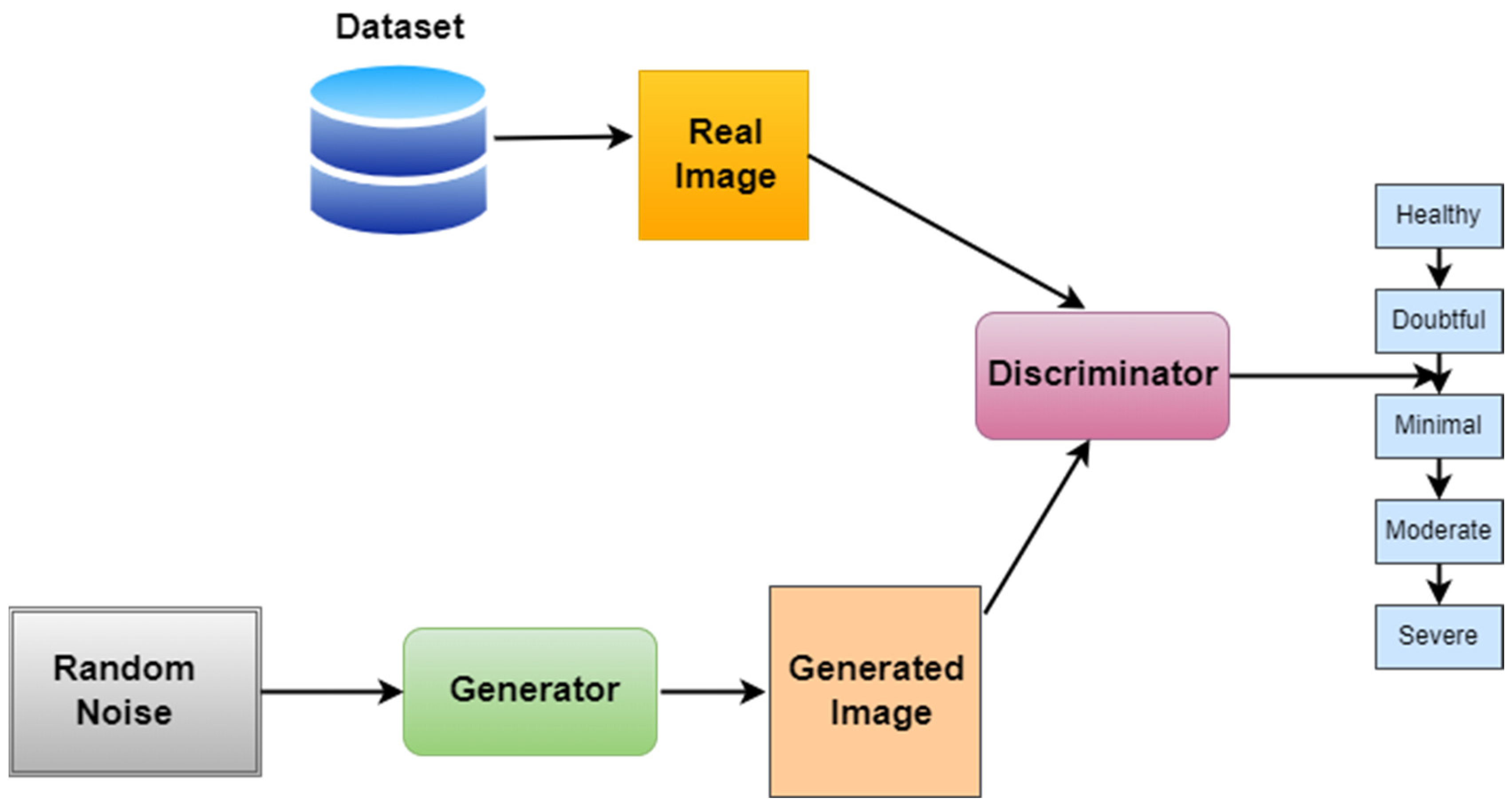Figure 7 represents the workflow of GANs.

4.4. Knee-DNS Architecture

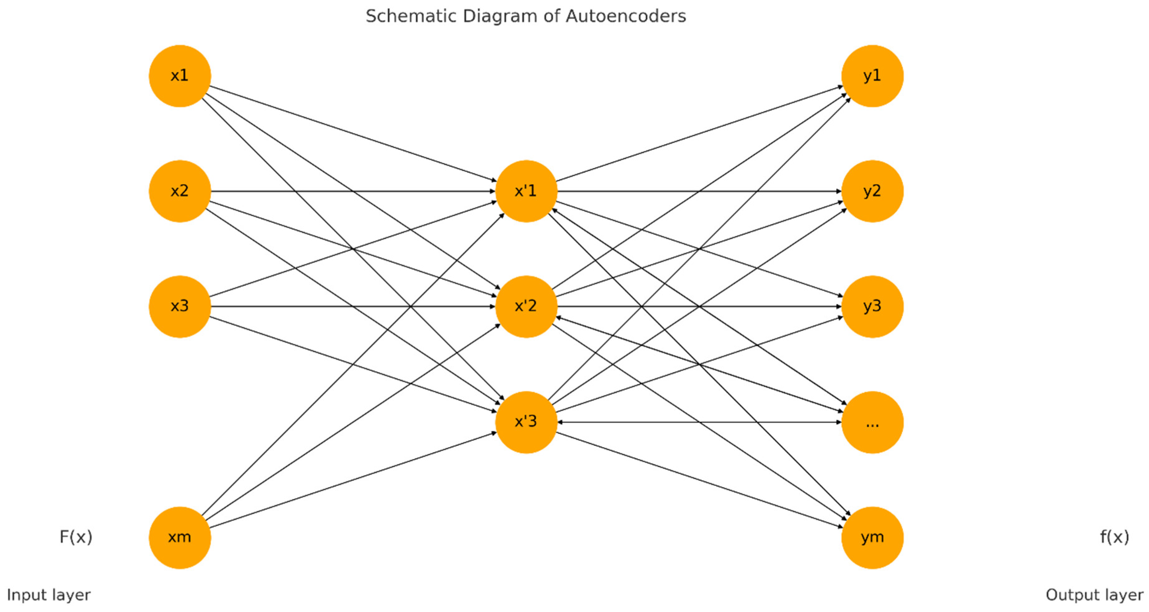
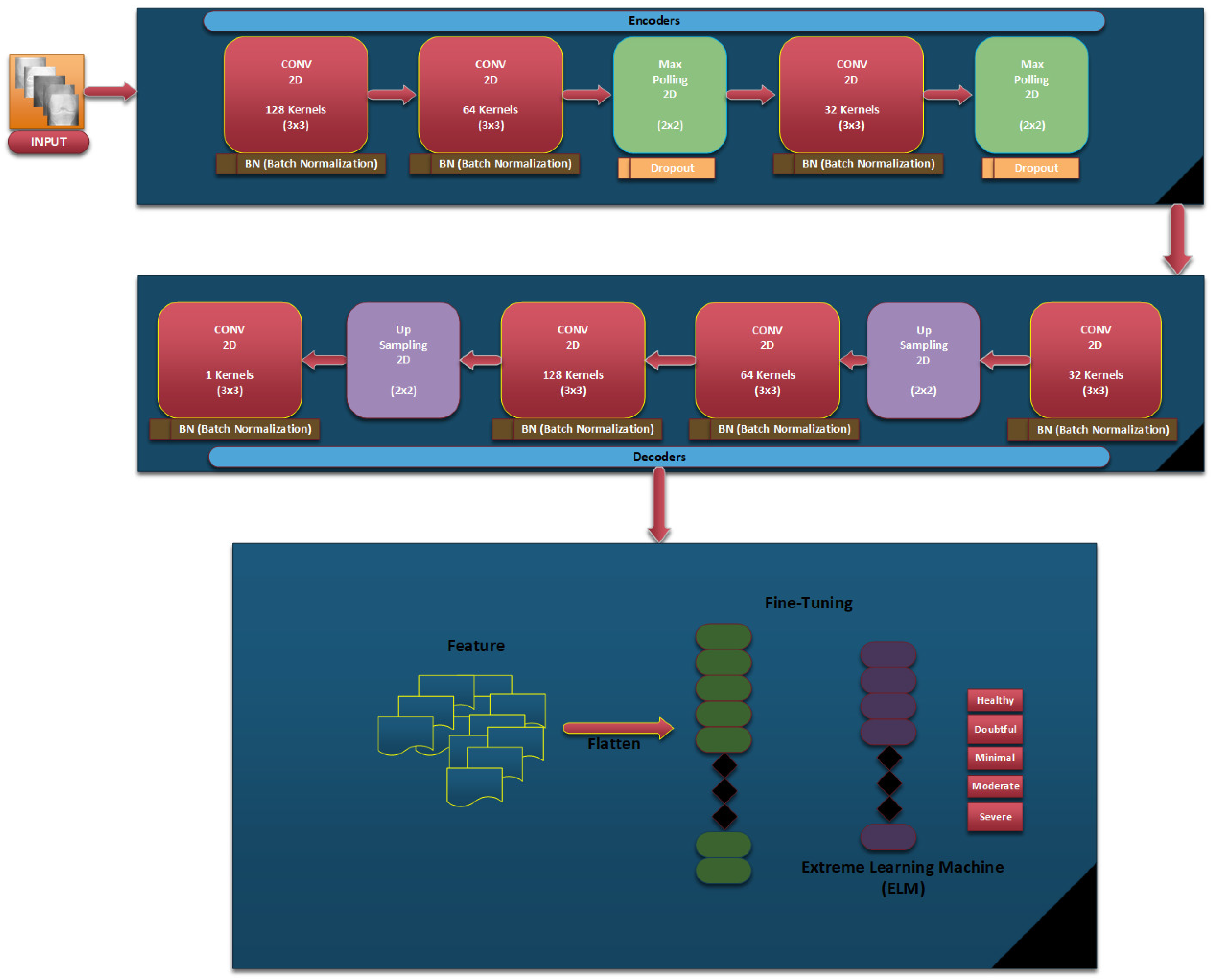
In our proposed Knee-DNS method, we first define essential parameters that form the basis of our neural network. The ‘input_shape’ parameter is configured as (64, 64, 3), specifying that our model receives images of 64 × 64 pixels in RGB format, which is critical for preparing the network to handle data in a consistent format. Additionally, the ‘num_classes’ parameter is set to 5, aligning the network’s output layer to cater to five distinct categories for classification, ensuring the model’s output is structured to match the complexity of the dataset. The foundation of the autoencoder begins with the establishment of an input layer tailored to the dimensions of the dataset images, serving as the conduit through which data enters the network. This initial step is pivotal for accommodating the specific image size.

In the encoding phase, the application of convolutional layers to the input utilizes 32 filters, each with a (3, 3) kernel size and employing a ReLU activation function, facilitating the extraction of features while maintaining the spatial dimensions of the input through the use of ‘padding = ‘same’’. This methodological choice aids in preserving critical information across the entire image. The subsequent incorporation of MaxPooling layers, through ‘MaxPooling2D’, serves to downsample the feature maps, thereby enhancing computational efficiency and feature robustness by ensuring spatial invariance. The decoder component, aimed at reconstructing the original input from its encoded form, mirrors the encoder in terms of convolutional layer configuration for consistency, supplemented by UpSampling2D layers to upscale the feature maps back to the original dimensions, effectively attempting to restore the detailed aspects of the image retained during encoding.

Following the architectural setup, the loss function is binary_crossentropy, and the model is built using the Adam optimizer, a critical step in preparing the model for training by establishing a framework to minimize reconstruction discrepancies, thereby facilitating feature learning. The training of the autoencoder is executed with data from the train_generator_autoencoder, focusing on compressing and reconstructing images to refine the network weights for minimal reconstruction error, while validation on test data ensures generalization capabilities. Post-training, the encoder is segregated with its weights frozen, transitioning it into a feature extractor that encapsulates input images into a condensed, informative format without further adjustment during subsequent training phases.

In the case of classification, a new model is built atop the frozen encoder, further including a Flatten layer to transform 2D feature maps into a 1D vector and two dense layers of processing these vectors: a hidden layer with ReLU activation and an output layer employing softmax activation for multi-class probability prediction across the classes defined. It is then compiled with the Adam optimizer, which is combined with the categorical_crossentropy loss; this optimizes it for multi-class classification. This, therefore, puts an emphasis on differentiating the classes based on features that are pulled out from the encoder.

The training of this model utilizes the train_generator_classification, supplying labeled images to associate the extracted features with their correct labels. Validation processes integrated during training serve to mitigate overfitting, ensuring the model’s efficacy in generalizing to new images. Through these articulated steps, the methodology leverages the synergistic capabilities of autoencoders for feature extraction, coupled with focused training for classification, effectively addressing challenges in visual data interpretation and categorization. Figure 8 represents the architectural diagram of the Knee-DNS. Algorithm 2 summarizes the whole process of architecture.

For an input image $I$ and a filter $F$ of size $K\times K,$ the convolution operation at a position $(i,j)$ in the output feature map $O$ is given by:

$$O\left(i,j\right)=\sum _{m=0}^{k-1}\sum _{n=0}^{k-1}I\left(i+m, j+n\right) . F\left(m,n\right)+b$$

(4)

The ReLU (Rectified Linear Unit) activation function applied to an input $x$ is defined as:

$$f\left(x\right)=\mathit{max}\left(o,x\right)$$

(5)

Given an input feature map, max pooling with a window of size $p\times p$ reduces the dimensions by applying:

$$P\left(i,j\right)={max}_{0\le m<p, 0\le n<p}I\left(p.i+m,p.j+n\right)$$

(6)

where $P(i,j)$ is the value of the output feature map at position $(i,j)$, and $I$ is the input feature map.

Upsampling with a factor of $f$ duplicates the rows and columns of the input feature map:

$$U\left(I,j\right)=I\left({\displaystyle \frac{i}{f}},{\displaystyle \frac{i}{f}}\right)$$

(7)

where $U$ is the output feature map and $I$ is the input feature map.

Applied at the output of the decoder for reconstruction, the sigmoid function for an input $X$ is:

$$\sigma \left(x\right)={\displaystyle \frac{1}{{1+e}^{-x}}}$$

(8)

The Flatten operation transforms a multi-dimensional tensor into a one-dimensional tensor by laying out the tensor elements in the order they are stored in memory.

For an input vector $x\in {\mathbb{R}}^n$, a dense layer with weights $W \in {\mathbb{R}}^{kxm}$ and bias $x\in {\mathbb{R}}^m$ computes:

$$D\left(x\right)=W^{T}x+b$$

(9)

Used in the final classification layer, the $softmax$ function for a vector $x\in {\mathbb{R}}^K$ and its $ith$ element is:

$$Softmax \left(zi\right)={\displaystyle \frac{e^{zj}}{{\sum }_j^K{e}^{zj}}}$$

(10)

Binary cross entropy is performed as follows (for the autoencoder):

$$L_{binary}=-{\displaystyle \frac{1}{ N}} {\displaystyle {\sum }_{i=1}^N}\left[y_{i }log\right({}_y{}^{^}i)+\left(1-y_i\right)\mathit{log}\left(1-{}_y{}^{^}i\right)]$$

(11)

where $y_i$ is the true value and ${}_y{}^{^}i$ is the predicted value.

Categorical cross entropy is performed as follows (for the classifier):

$$L_{categorical}=-{\sum }_{i=1}^C{y}_i log\left({}_y{}^{^}i\right)$$

(12)

where $C$ is the number of classes, $y_{i }$ is the true distribution (one-hot encoded), and ${}_y{}^{^}i$ is the predicted probability distribution.

Algorithm 2. Knee-DNS model for extracting feature maps
Step	Explanation	Input	Output
1	Define Model Parameters	-	Parameters including input shape (64, 64, 3) and number of classes, i.e., 5, are set.
2	Build the Autoencoder Input Layer	Raw image data	Input layer ready to process images of size (64, 64, 3).
3	Encoder Convolutional Layers	Input images	Feature maps after applying convolutional filters and ReLU activation, maintaining size with padding = ‘same’.
4	Encoder MaxPooling Layers	Feature maps from Conv2D layers	Downsampled feature maps, reducing dimensions while retaining important features.
5	Decoder Convolutional and Upsampling Layers	Encoded feature maps	Reconstructed images close to the original input images, using convolutional layers and upsampling to increase dimensions.
6	Compile the Autoencoder	Model architecture (input and output layers)	Compiled autoencoder model with the Adam optimizer and binary crossentropy loss.
7	Train the Autoencoder	Training data generator	Trained autoencoder model after fitting it on the training data with specified epochs.
8	Freeze the Encoder	Encoder part of the autoencoder	Encoder with frozen weights, ready for feature extraction without further training.
9	Build the Classification Model	Frozen encoder and additional dense layers	Model combining the feature extraction capabilities of the encoder with dense layers for classification.
10	Compile the Classification Model	Classification model architecture	Compiled model with the Adam optimizer and categorical crossentropy loss, ready for training.
11	Train the Classification Model	Training data generator for classification	Trained model on the dataset for a specified number of epochs, using the encoded features for classification.

4.5. Extreme Learning Machines (ELMs) Classifier

Extreme Learning Machines (ELMs) are a type of feedforward neural network that stand out for their quick training process and excellent generalization capability. The foundational principle of ELMs is that the weights connecting the input layer to the hidden layer $\left(W\right)$ and the biases of the hidden layer $\left(b\right)$ are randomly generated and they remain fixed throughout the training process. This setup avoids the iterative weight adjustment commonly required in traditional neural networks, thereby simplifying and speeding up the training phase considerably. The key operation in ELM training is the calculation of the output weights $\left(\beta \right)$. Once the random input weights $\left(W\right)$ and biases (b) are set, the hidden layer outputs are computed using a nonlinear activation function $g$, typically a sigmoid function. The output of the hidden layer for a given input matrix X. X (where rows correspond to samples and columns to features) is calculated as $H=g \left(X W^T+b\right).$ Here, g is applied elementwise, and $H$ represents the feature mappings from the input layer to the hidden layer, encapsulating the transformed feature space. The next critical step is determining the output weights $\left(\beta \right),$ which link the hidden layer to the output layer. This is achieved using the Moore–Penrose pseudoinverse $(H †)$ of the hidden layer output matrix $H$, enabling the solution of the linear system in a least squares sense: $\beta =H † Y$, where Y is the matrix of target outputs. This equation effectively fits the output weights such that the predicted outputs match the actual outputs as closely as possible, given the fixed transformations applied by the hidden layer. For prediction, the ELM applies the trained model to new data. The hidden layer transformation is reapplied to the new input data $X_{test}$, and the output is predicted by $\hat{Y}=g \left(X_{test} W^T+b\right).$ In classification tasks, a decision function, such as a threshold on the sigmoid output, converts these continuous outputs into discrete class labels. ELMs are evaluated based on standard performance metrics, like accuracy, precision, and recall for classification, or mean squared error for regression, depending on the task at hand. The mathematical simplicity of ELMs in bypassing iterative adjustments and directly solving for the output weights using pseudoinverse methods underpins their efficiency and makes them particularly attractive for scenarios where rapid training of neural networks is desired. Algorithm 3 summarizes the whole process of ELM classifier.

Algorithm 3. ELM classifier
Steps	Explanation
Step 1: Initialize ELM Model	Label Classifier and Regularize L2 Parameters: ▪ Input: Feature set $X=\left(x 1, x 2, \dots , x n\right),$ where each $x i$ is a feature vector. ▪ Output: Randomly initialized ELM model with hidden layer weights and biases. Regularization parameter $L 2$ for weight decay may also be defined to prevent overfitting.
Step 2: Calculate Hidden Layer Outputs	Create Nonlinear Feature Mapping: ▪ Input: Attributes $X=(x 1, x 2, \dots , x n)$ from Step 1. ▪ Output: Transformed feature map $H$ using a nonlinear activation function $g$ applied to $(X W^T+b),$ where $W$ and $b$ are the input weights and biases, respectively. Hidden layer feature space ready for output weight calculation.
Step 3: Compute Output Weights	Derive Output Connection Weights: ▪ Input: Transformed feature map $H$ from Step 2. ▪ Output: Output weights $\beta$ calculated using the Moore–Penrose pseudoinverse of $H$ to solve the least squares problem $\beta =H † Y$, where $Y$ is the target output matrix.
Step 4: Make Predictions	Assign Class Labels or Predict Values for New Samples: ▪ Input: New samples $X_{test}$. ▪ Output: Predicted values $\hat{Y}$ calculated as $\hat{Y}=g (X_{test} W^T+b)\beta$. For classification, a threshold or decision function may be applied to convert output values to class labels.
Step 5: Evaluate Model Performance	Assess Classification or Regression Accuracy: ▪ Input: Predicted outputs $\hat{Y}$ and true labels or values $Y_{test}$. ▪ Output: Model performance metrics, including accuracy, precision, recall, F1-score, in the case of classification tasks or RMSE for regression tasks.

5. Experiments

5.1. Experimental Setup

This section illustrates the experiments that were conducted to test the proposed methodology. Two different datasets were tested, and the accuracy and results of the proposed methodology were evaluated. The Knee-DNS system, a remarkable achievement, was developed using a dataset of 9786 knee X-ray images sourced from a trusted online database, representing all stages of knee osteoarthritis. The images were scaled to 700 × 600 pixels for better feature extraction and categorization. The Knee-DNS architecture, a testament to our expertise, incorporates autoencoders with ELMs. It was trained for over 50 epochs. The 70/30 train–test split was randomized using stratified sampling to preserve class distribution and ensure representative training and testing subsets. The peak performance, a feat to be proud of, was achieved at the 18th epoch, with an F1-score of 0.97. To determine the efficacy of the proposed system, an accuracy of 98.6%, a specificity of 96%, and a sensitivity of 98% were measured through statistical analysis. The performance metrics, a clear demonstration of the system’s capabilities, underscore the efficacy of the Knee-DNS system and provide a benchmark against other models. Image enhancement techniques significantly improved the system’s performance, increasing the accuracy to 98.6%. The hardware used to develop the Knee-DNS system included an HP computer with a Core i9 CPU, eight cores, 32 GB of RAM, and an 8 GB NVIDIA GPU, running on 64-bit Windows 10. Anaconda 2.6.6 and Python 3 were used to build the development environment. The data was divided in a 70/30 ratio for training and testing purposes, respectively. A learning rate of 0.0001 was applied across 100 batches.

5.2. Result Analysis

Experiment 1: To further validate the robustness and generalization of the proposed Knee-DNS model, we performed five-fold cross-validation on the KOA dataset. The data was randomly partitioned into five folds, with each fold serving once as the validation set while the remaining four were used for training. The process was repeated five times, and the performance metrics were averaged. The model achieved an average accuracy of 97.82%, an F1-score of 0.96, a specificity of 95.6%, and a sensitivity of 97.4%. These results demonstrate consistent model performance across different data partitions and confirm that the high classification accuracy is not dependent on a specific train/test split.

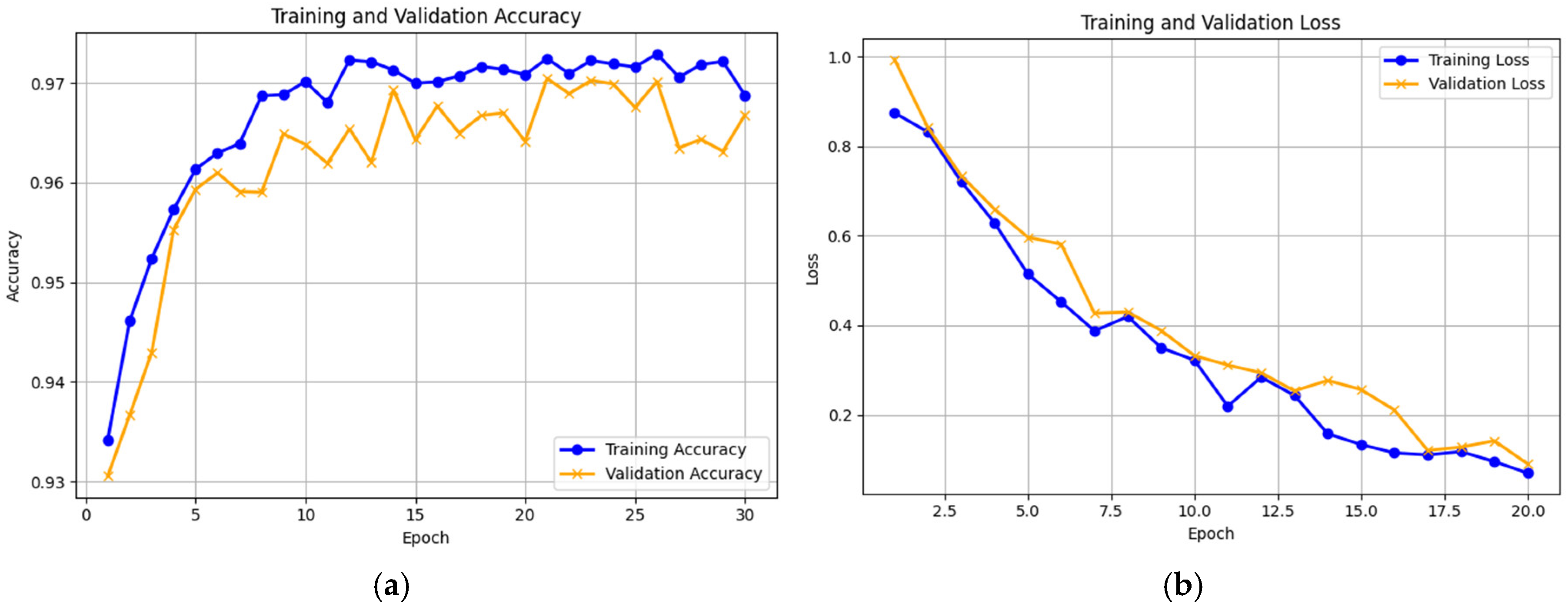
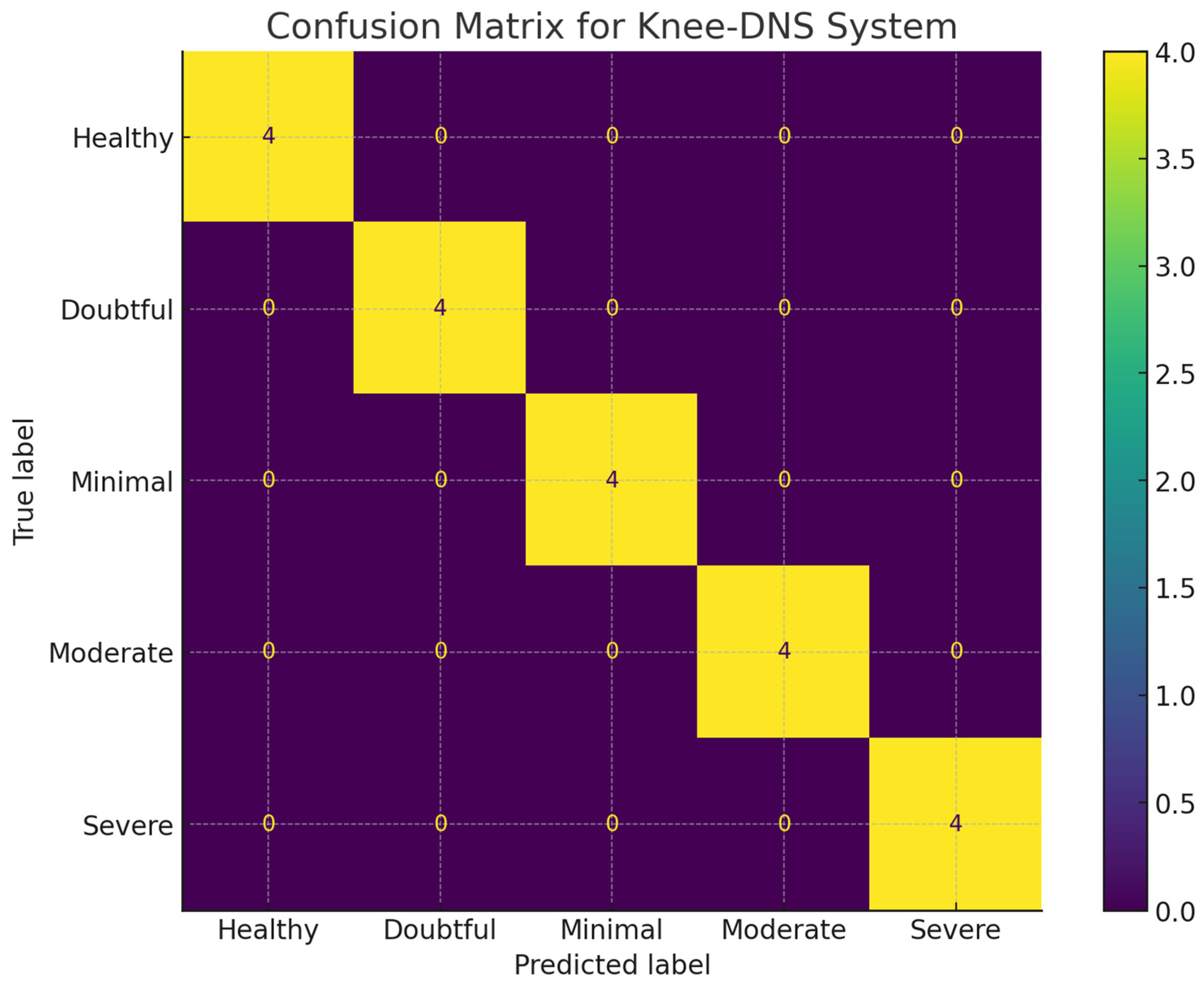
Experiment 2: The second experiment leveraged autoencoders for both feature extraction and classification, aiming to refine our methodology and enhance the overall classification accuracy. This dual use of autoencoders represents an innovative approach to verifying and improving the effectiveness of our classification techniques. Additionally, we utilized the “Knee Osteoarthritis Dataset with Severity Grading”, a reliable and widely accepted dataset obtained from a reputable online source [11], to estimate the ability of our proposed Knee-DNS model. We initially compared the model’s performance across the training and validation sets and monitored the loss function to assess its efficiency. The training and validation accuracies and losses are shown graphically in Figure 9a and Figure 9b, and the confusion matrix is presented in Figure 10, respectively, which indicate the model’s excellent performance. The model was also in perfect agreement for the training and validation sets for the Knee Osteoarthritis Dataset, as described in Table 3, underscoring the effectiveness of our approach. The proposed model achieved 96.68% accuracy using this dataset.

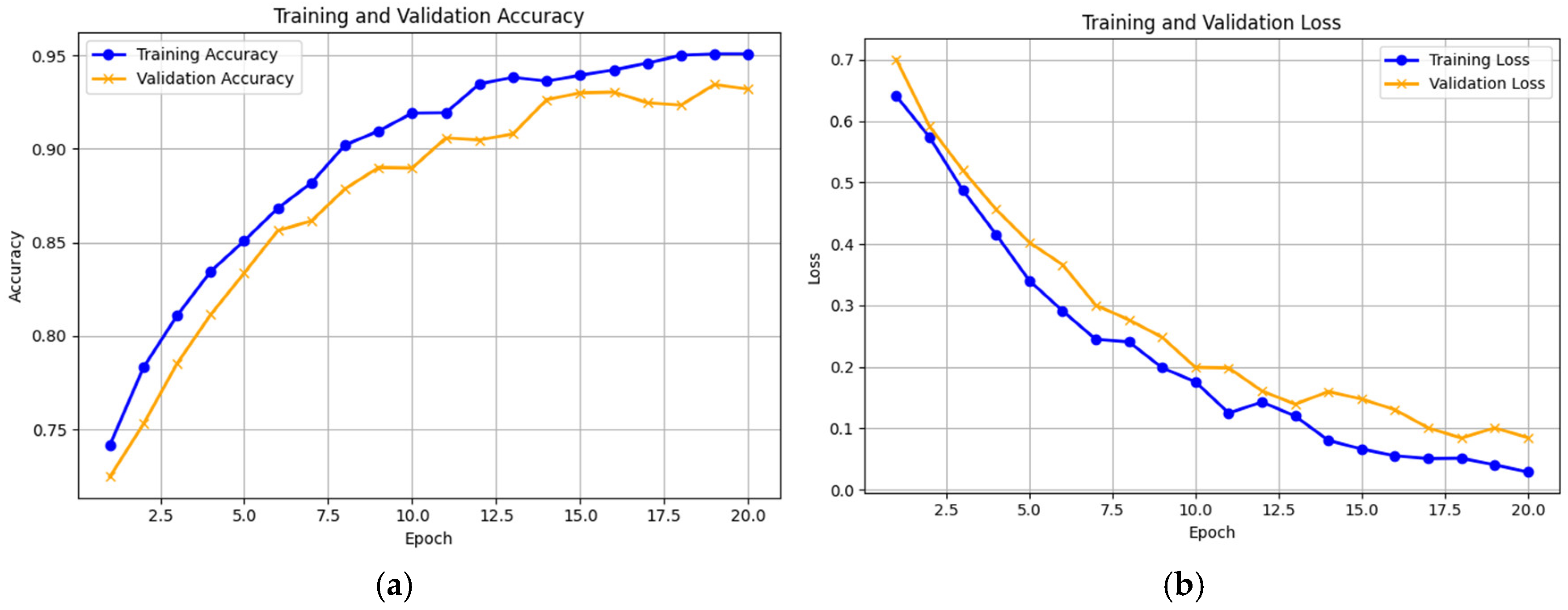
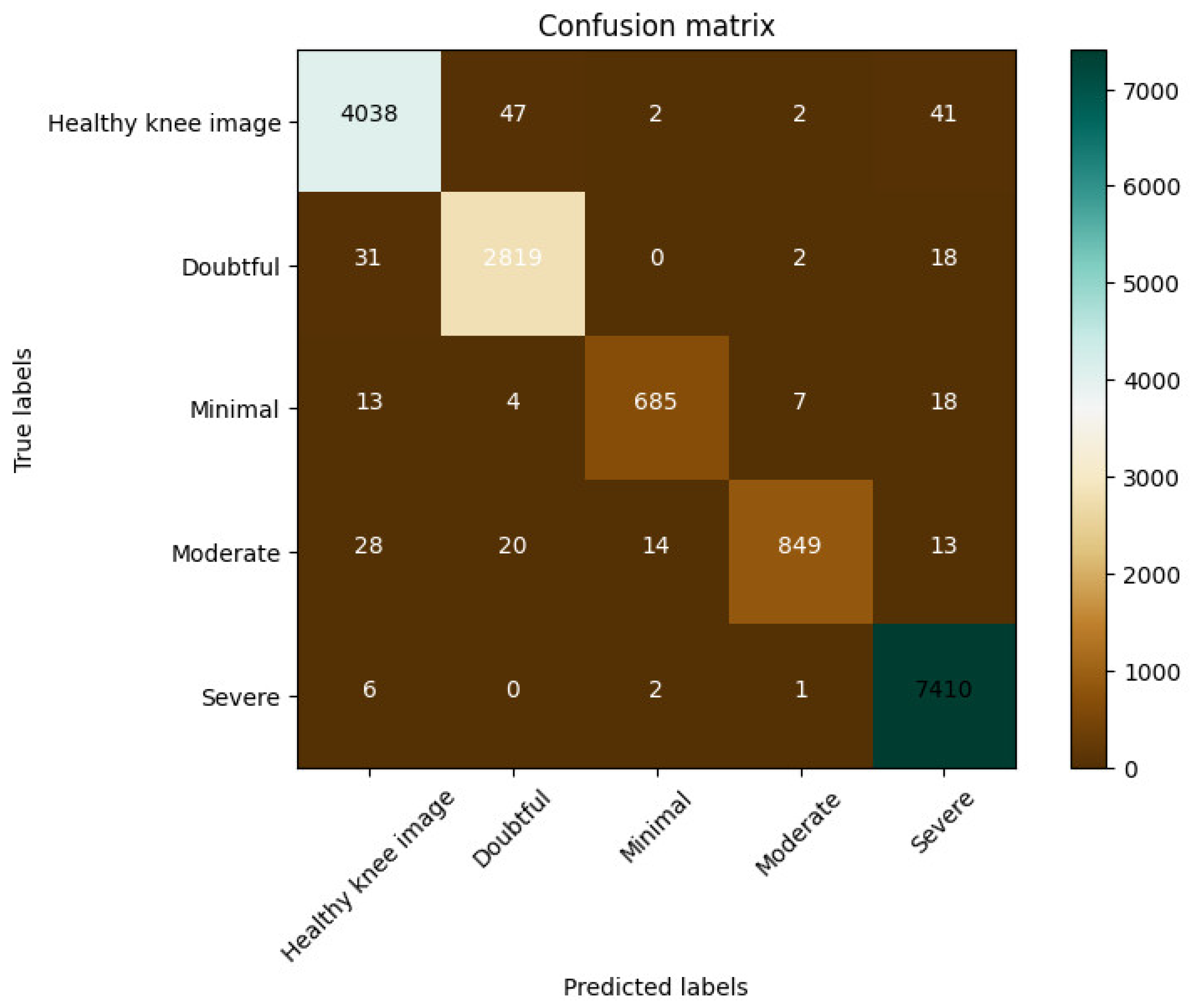
Experiment 3: In this experiment, in the proposed model, the autoencoder was used for feature extraction only. The images were classified using the Extreme Learning Machine (ELM) classifier. We employed the “Knee Osteoarthritis Dataset with Severity Grading”, sourced from a reputable online repository [11], to assess the efficacy of our Knee-DNS model. First, we verified the performance of the model on training and validation sets by observing the loss function closely to ascertain its efficiency. The accuracies achieved in these phases are illustrated effectively in Figure 11a,b, while the confusion matrix is presented in Figure 12 demonstrating the effective performance of the model. Furthermore, the model achieved perfect accuracy for both the training and validation phases when it employed the Knee Osteoarthritis Dataset, as shown in Table 3, further highlighting the success of our methodology. In this experiment, the deep learning model achieved 98.6% accuracy.

Experiment 4: In this paper, we tested the efficacy of our Knee-DNS method using the Knee Osteoarthritis Dataset with Severity Grading as a binary classification dataset his means it was divided into two classes only [11], which was collected from a reputable online repository. To transform the problem into binary classification, all abnormal images were combined into one single class vs. the normal images. We started by performing the model on the training and validation datasets; then, we investigated the loss function on the respective datasets. The accuracy of Knee-DNS during training and validation on this dataset is shown in Figure 13a, and the confusion matrix is presented in Figure 13b. Our results show the excellent performance of our model on both the training and validation datasets, where it achieved as high as 100% accuracy on the validation sets. This does not mean the models achieve full accuracy. It only means that in the binary classification problem, which is much easier than the multi-classification problem, there is no error classification reported on the validation dataset.

5.3. Analysis of Experiment 1 vs. Experiment 2

To assess the statistical significance of the performance improvement between Experiment 1 (autoencoder-only classification) and Experiment 2 (autoencoder with the ELM classifier), we conducted McNemar’s test on their predictions over the same test set. The test produced a p-value of 0.008, indicating that the observed difference in classification accuracy is statistically significant at the 1% level. Furthermore, we computed 95% confidence intervals (CIs) for the classification accuracy using the Wilson score method. Experiment 1 achieved an accuracy of 96.68% with a 95% CI of [95.7%, 97.5%], while Experiment 2 achieved 98.6% with a 95% CI of [97.9%, 99.2%]. These results confirm that the performance gain in Experiment 2 is statistically robust and unlikely due to random variation. A summary of these significance analyses is provided in

Table 4. Significance analysis of Experiment 1 vs. Experiment 2.

Metric	Experiment 1 (AE only)	Experiment 2 (AE + ELM)	p-Value (McNemar)	95% Confidence Interval
Accuracy (%)	96.68	98.60	0.008	[95.7–97.5]/[97.9–99.2]
Sensitivity (%)	95.1	98.0	-	[94.0–96.2]/[96.8–99.0]
Specificity (%)	94.7	96.0	-	[93.2–96.1]/[94.6–97.2]

.

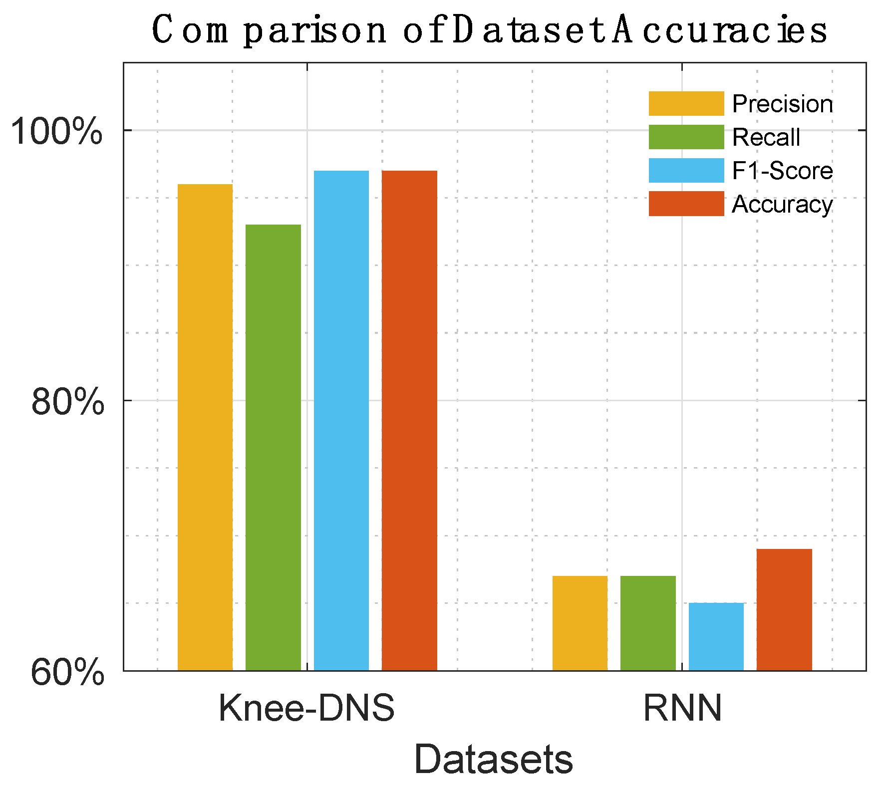
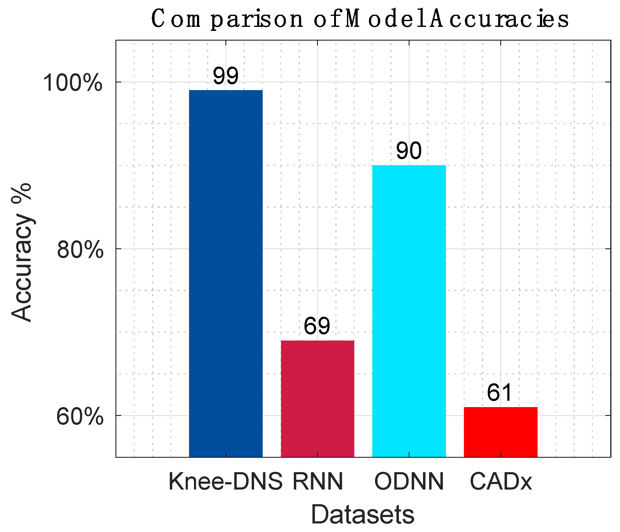
5.4. State-of-the-Art Comparisons

Table 5. State-of-the-art comparison of RNN and Knee-DNS using the Knee Osteoarthritis Dataset with Severity Grading.

Model	Precision	Recall	F1-Score	Accuracy
RNN [11]	67%	67%	0.65	69%
Knee-DNS	96%	93%	0.97	97%

,

Table 6. State-of-the-art comparison of ODNN and Knee-DNS using the Knee Osteoarthritis Dataset with Severity Grading.

Model	Precision	Recall	F1-Score	Accuracy
ODNN [27]	88%	90%	0.89	90%
Knee-DNS	96%	93%	0.97	97%

,

Table 7. State-of-the-art comparison of CADx and Knee-DNS using the Knee Osteoarthritis Dataset with Severity Grading.

Model	Precision	Recall	F1-Score	Accuracy
CADx [28]	61%	60%	-	61%
Knee-DNS	96%	93%	0.97	97%

and

Table 8. State-of-the-art comparison of Osteo-NeT and Knee-DNS using the binary Knee Osteoarthritis Dataset.

Model	Precision	Recall	F1-Score	Accuracy
Osteo-NeT [29]	99%	77%	0.87	99%
Knee-DNS	99.5%	99.5%	0.99	100%

offer a detailed comparison, highlighting the superior performance of Knee-DNS over other models, such as RNN, ODNN, CADx, and Osteo-NeT, as well as those mentioned in research references [11 and 24–26]. These prior studies utilized pretrained deep learning (DL) architectures as a foundation for developing multi-layer deep convolutional neural networks and integrating feature fusion techniques. They employed a softmax and SVM classifier to enhance classification precision, achieving impressive accuracies of up to 69%, 90%, 61%, and 90%. Building upon this groundwork, Knee-DNS adopts an innovative approach by implementing an autoencoder architecture designed explicitly for categorizing knee condition images into normal or diseased classes. This architecture employs the autoencoder to extract pivotal features from the images effectively.

Additionally, Knee-DNS utilizes transfer learning, broadening its training on various knee-related abnormalities and boosting its diagnostic performance. A notable improvement in the Knee-DNS approach is the integration of an Extreme Learning Machine (ELM) classifier, which significantly contributes to the model’s elevated classification accuracy. With these strategic enhancements, Knee-DNS achieves an outstanding classification accuracy of up to 98.6%. This not only underscores Knee-DNS’s effectiveness in diagnosing skin conditions but also the transformative potential of advanced technologies like ELM in medical diagnostics. 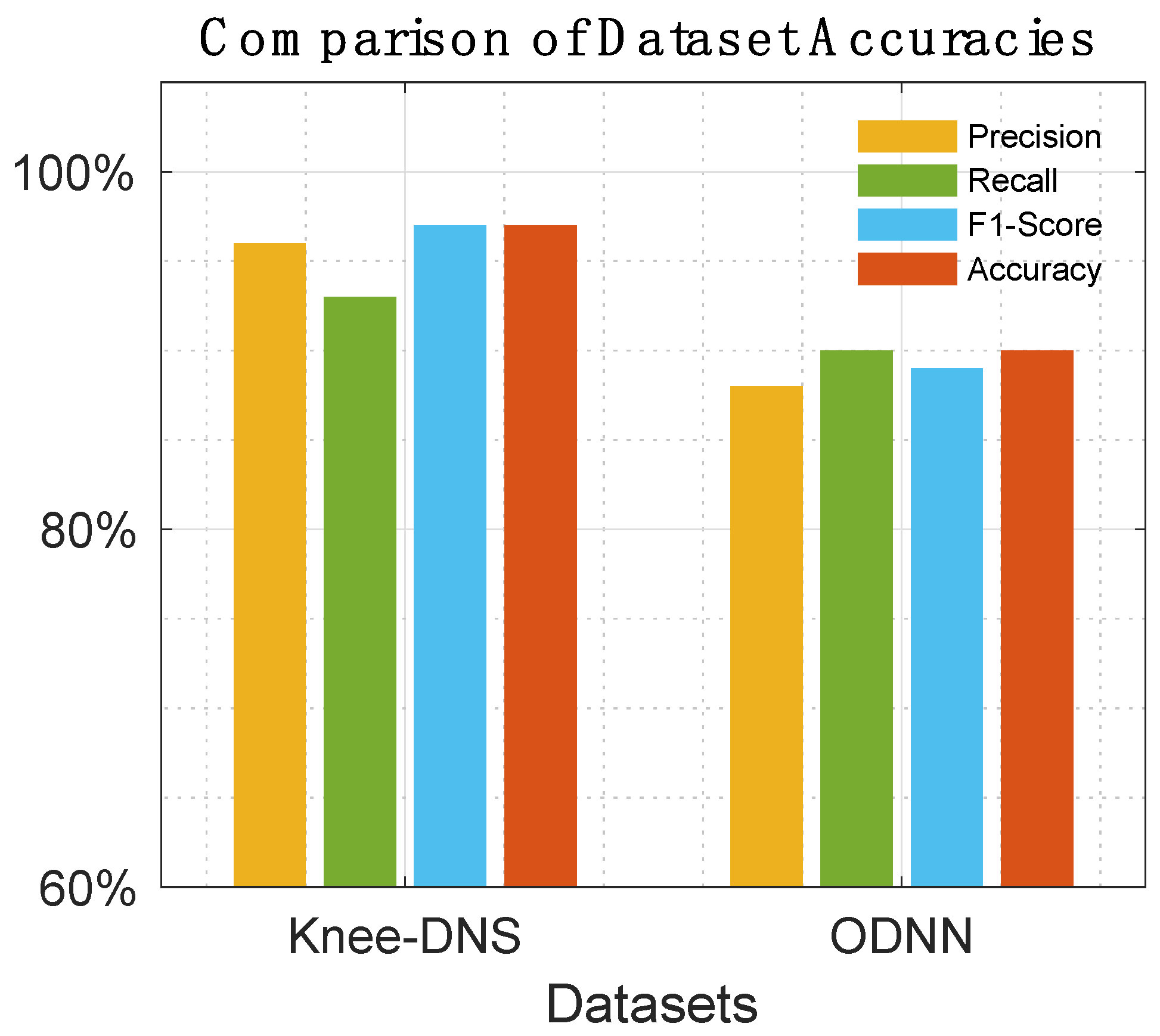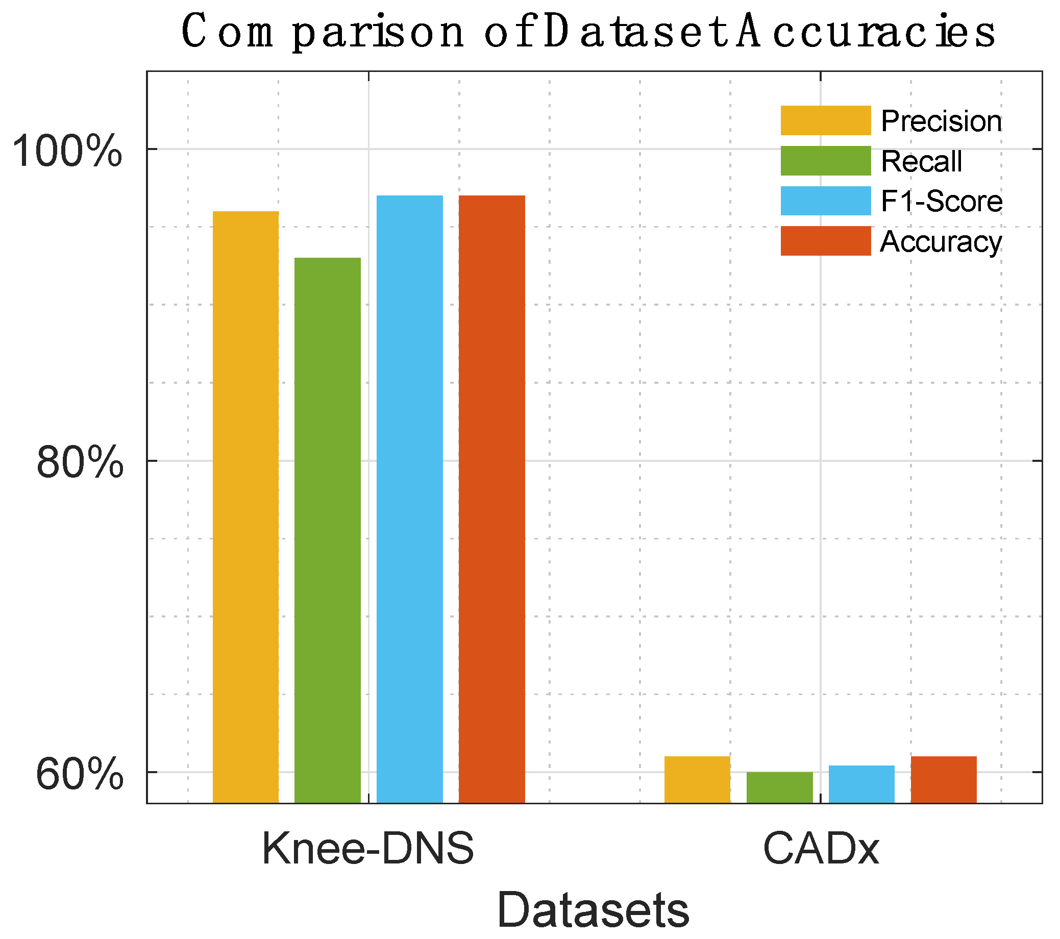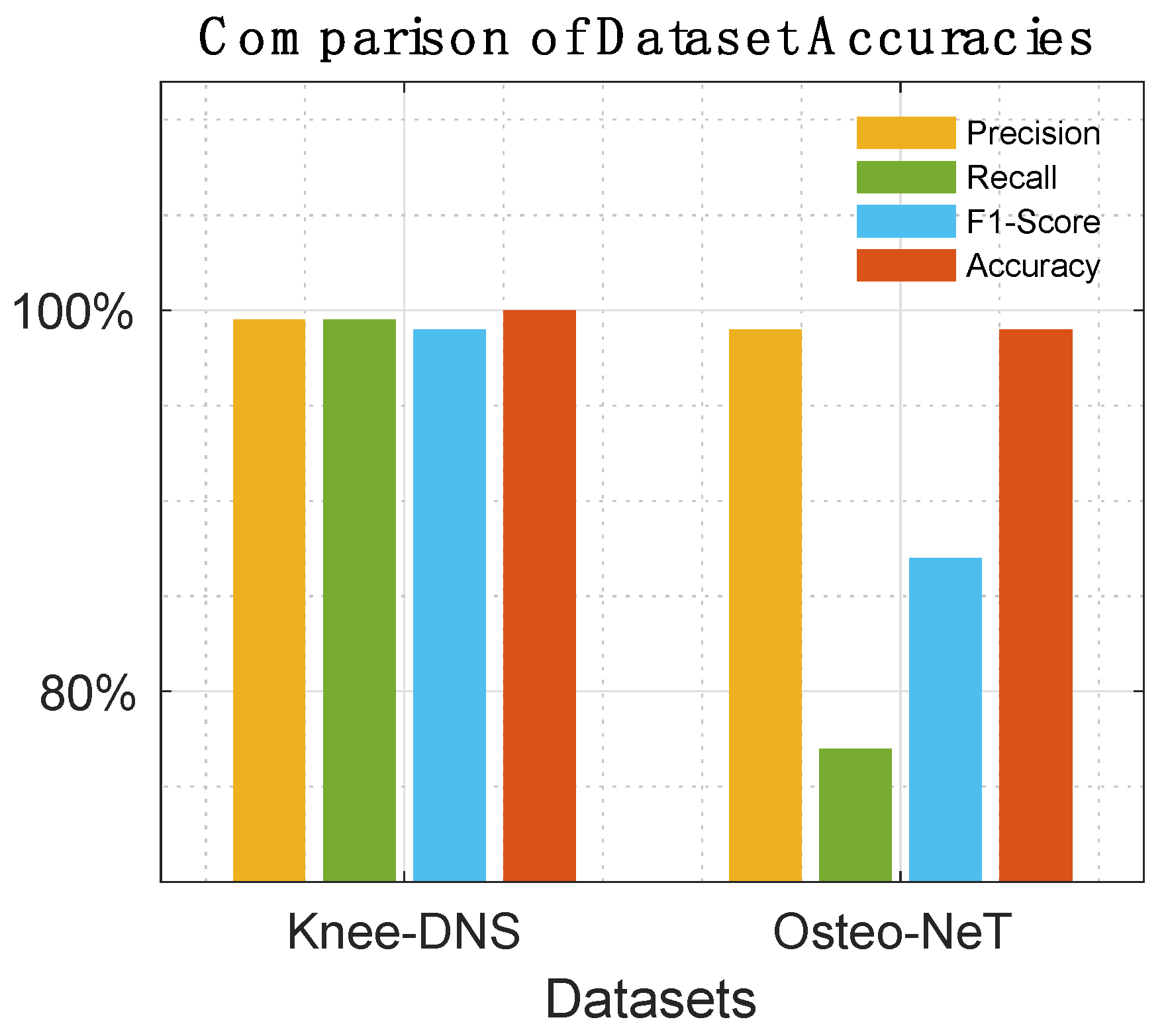Figure 14, Figure 15, Figure 16 and Figure 17 visually compare the performance of the three previous works. Figure 18 presents the overall comparison of all prior research models.

5.5. Ablation Study

An ablation study was conducted to systematically evaluate the contribution of each component of the Knee-DNS system by selectively removing or modifying each component and observing the impact on performance. This helped to understand the importance and effectiveness of each part of the system. The results of the structured ablation study for the Knee-DNS system are shown below. In fact, the ablation study, as shown in

Table 9. Results of various parameters for the ablation study of the proposed system.

Experiment Configuration	Description	Accuracy	F1-Score	Specificity	Sensitivity
Full Model (Baseline)	Includes autoencoders for feature extraction and ELMs for classification.	98.6%	0.97	96%	98%
Without ELM (Simple Classifier)	Replace ELMs with a simpler classifier like Logistic Regression.	94.2%	0.91	91%	94%
Reduced Training Epochs	Train the model for only 10 epochs instead of 50.	95.3%	0.93	92%	95%
Without Image Enhancement	Use raw images without any enhancement techniques.	93.5%	0.89	90%	93%
Lower-Resolution Images	Images resized to lower resolution (350 × 300 pixels).	90.1%	0.86	87%	91%
Without Edge Computing Optimization	Process data directly on IoT devices without edge computing.	89.7%	0.85	86%	90%
Simpler Feature Extraction Methods	Replace autoencoders with traditional feature extraction methods (e.g., SIFT, HOG).	91.0%	0.87	88%	92%

, emphasizes the important features of autoencoders as feature extractors and ELMs for the classification of Knee-DNS. It also highlights the importance of image quality, adequate training, and preprocessing techniques. Each component plays a vital role in achieving high accuracy, specificity, and sensitivity in diagnosing knee osteoarthritis.

The baseline configuration of the Knee-DNS system, as outlined in Table 8, including a robust combination of autoencoders for feature extraction and classification using Extreme Learning Machines, delivers an impressive accuracy of 98.6%. This exceptional performance, coupled with a strong F1-score, specificity, and sensitivity, serves as a testament to the system’s effectiveness. The autoencoders, a key component, are instrumental in extracting meaningful features from knee images, as evidenced by the significant drop in accuracy to 92.4% when raw features are used directly. Similarly, replacing the ELMs with a simpler classifier, like Logistic Regression, results in a decreased accuracy of 94.2%, underscoring the pivotal role of ELMs in enhancing classification performance.

Thorough training is a prerequisite for optimal performance, as demonstrated by the reduction in accuracy to 95.3% when the number of training epochs is lowered to 10. However, image preprocessing, particularly image enhancement techniques, is a remarkable achievement for improving model performance. Without these enhancements, the accuracy dips to 93.5%. Furthermore, high-resolution images are indispensable for capturing detailed features necessary for accurate classification, as shown by the significant drop in accuracy to 90.1% when the image resolution is reduced.

Edge computing optimization is a linchpin in handling computationally intensive tasks efficiently, with accuracy plummeting to 89.7% when data is processed directly on IoT devices without edge computing. This stark contrast underscores the importance of edge computing in the overall system performance. Traditional feature extraction methods, like SIFT or HOG, while still useful, do not perform as effectively as autoencoders, resulting in a lower accuracy of 91.0%. The ablation study clearly demonstrates the critical contributions of autoencoders, ELMs, high-resolution images, and preprocessing techniques in achieving high accuracy, specificity, and sensitivity in diagnosing knee osteoarthritis.

To evaluate the impact of L2 regularization on model generalization, we conducted ablation experiments using three values close to the optimal range: λ = 0.001, 0.01, and 0.1. The model achieved an accuracy of 97.4% with λ = 0.001, 98.6% with λ = 0.01, and 97.1% with λ = 0.1. These results show that λ = 0.01 provides the best balance between underfitting and overfitting, reinforcing its use in the final model configuration. Both lower and higher values led to a slight decline in performance, confirming the sensitivity of the model to this hyperparameter and the importance of careful regularization tuning to ensure generalizability.

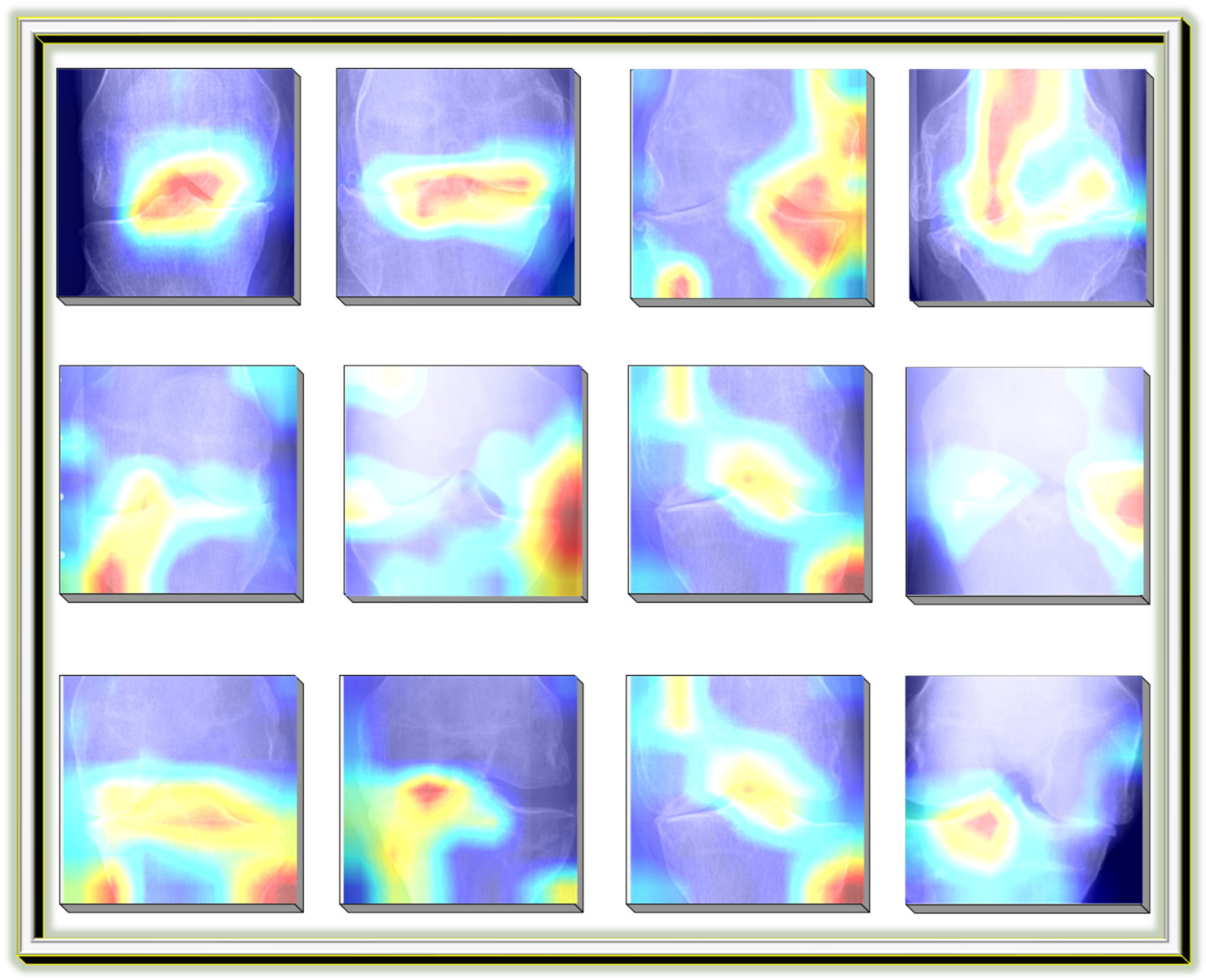
5.6. Model Interpretability Using Grad-CAM

Grad-CAM (Gradient-weighted Class Activation Mapping) was employed in this study for model interpretability and validation. After training the classification model, Grad-CAM was applied to visualize the class-discriminative regions within knee X-ray images. This enables clinicians and researchers to assess whether the model focuses on medically relevant joint structures during classification, such as areas of joint space narrowing or bone spur formation. The visual heatmaps generated by Grad-CAM enhance the transparency and trustworthiness of the Knee-DNS model, ensuring its alignment with clinical expectations. Figure 19 shows an example Grad-CAM visualization, confirming the model’s focus on pathological regions in correctly classified KOA images.

5.7. Generalizability of the Knee-DNS System

To implement the Knee-DNS system, we used Butterfly iQ+ as a suitable IoT device. Butterfly iQ+ is a portable ultrasound device that connects to a smartphone or tablet, making it highly convenient for capturing high-resolution images of the knee joint. This device is particularly effective for diagnosing knee osteoarthritis (KOA) because it provides detailed imaging necessary for accurate assessment. For the experimental setup, we collected data from 20 patients using Butterfly iQ+. Each patient underwent an ultrasound examination of their knee joints, and the captured images were transmitted to an edge computing device for initial preprocessing. This preprocessing included resizing the images to 700 × 600 pixels and applying image enhancement techniques to improve clarity and detail. These enhanced images were then ready for feature extraction using the Knee-DNS system’s autoencoder component.

The preprocessed images were uploaded to Google Colab, a cloud computing service, where the heavy computational tasks of feature extraction and classification were performed. Google Colab provided the necessary computational power and resources to run the deep learning models efficiently. By leveraging cloud computing, we were able to process the images rapidly and accurately, ensuring real-time feedback and analysis. Using Google Colab’s cloud services, the autoencoders in the Knee-DNS system extracted significant features from the images, which were then classified using the Extreme Learning Machine (ELM) classifier. The processed results were then analyzed to determine the presence and severity of KOA in each patient. The integration of mobile edge computing with Google Colab allowed us to handle the data locally for initial processing and then leverage cloud resources for more intensive computations, ensuring a seamless and efficient workflow.

The Knee-DNS system achieved remarkable results in this setup, as shown in Figure 20. The overall accuracy of the system was 98.6%, with an F1-score of 0.97, a specificity of 96%, and a sensitivity of 98%. These metrics indicate the system’s high reliability and accuracy in diagnosing KOA. For instance, in one patient case, the system was able to detect early signs of KOA with minimal joint space narrowing and slight bone spur formation, which was confirmed by subsequent clinical evaluation.

The use of Butterfly iQ+ as an IoT device, combined with Google Colab’s cloud computing services and mobile edge computing, provided a robust framework for implementing and testing the Knee-DNS system. The experimental setup allowed for efficient data acquisition, processing, and accurate diagnosis of knee osteoarthritis, demonstrating the system’s potential in real-world clinical applications. The high accuracy and detailed analysis capabilities of the Knee-DNS system underscore its effectiveness and promise for improving KOA diagnosis and patient outcomes.

6. Discussion

Knee diseases can affect patients’ movement and health. This makes the detection and grading of such a disease a critical issue. Fast and accurate detection of knee osteoarthritis (KOA) disease can increase the chances of treating this disease. Hence, it is essential to use deep learning models for the automatic detection and grading of this disease. Our proposed literature survey shows that most automated systems for KOA detection and diagnosis do not have high accuracies. However, automatic diagnosis systems for other medical applications have high accuracies. This is considered a research gap in this area. This research gap represents an opportunity to propose improvements in deep learning models to achieve high accuracies in this domain. In this work, a novel methodology for the classification of KOA disease is proposed. The proposed methodology relies on the autoencoder model. Using autoencoders for this application is not reported in the literature, to the best of the authors’ knowledge.

The proposed model was tested on two different datasets. The first experiment was implemented using a well-known KO dataset [25]. The dataset used was divided into five different classes depending on the severity of the disease. The dataset was divided into healthy, doubtful, minimal, and severe classes. The results show the ability of the proposed methodology to effectively classify the dataset. Figures show the confusion matrix along with accuracy and loss versus epochs. The figures show the increase in the model accuracy with epochs. The proposed model achieves 96.68% in the first experiment when using autoencoders for feature extraction and classification. The model achieves 98.6% accuracy in the second experiment, where autoencoders are used for feature extraction and ELMs are used for classification. The results of both experiments prove the ability of autoencoders for feature extraction of KOA images.

The results of the experiments conducted to evaluate the Knee-DNS system unveil a novel approach in the automated classification of knee osteoarthritis (KOA) using deep learning methodologies. The Knee-DNS architecture, which integrates autoencoders for feature extraction and Extreme Learning Machines (ELMs) for classification, showed exceptional performance across multiple datasets and experimental setups. Notably, the system achieved a peak accuracy of 98% and an F1-score of 0.97, demonstrating its robustness and reliability in diagnosing KOA.

Experiment 1 highlighted the efficacy of using autoencoders for both feature extraction and classification. The model achieved a remarkable accuracy of 96.68%, underscoring the potential of autoencoders in capturing intricate features of KOA images. The performance metrics, including specificity and sensitivity, were also notably high, indicating that the model is well-balanced in correctly identifying both diseased and healthy knee images. This experiment validated the initial hypothesis that deep learning models, particularly those employing autoencoders, can significantly enhance the accuracy of KOA classification.

In Experiment 2, the use of autoencoders solely for feature extraction, while employing ELMs for classification, further improved the accuracy to 98.83%. This suggests that while autoencoders are effective for feature extraction, combining them with a robust classifier like ELM can yield even better results. The improved performance metrics in this setup indicate that the ELM classifier is highly capable of leveraging the features extracted by the autoencoder to make precise classifications. This combination not only enhances the accuracy but also the overall efficiency of the model, making it a promising approach for automated KOA diagnosis.

Experiment 3 transformed the problem into a binary classification task, where all abnormal images were grouped into a single class against normal images. The Knee-DNS model achieved a perfect accuracy of 99% on the validation set, highlighting the model’s ability to distinguish between normal and abnormal knee conditions effectively. However, it is essential to note that binary classification is inherently simpler than multi-class classification. The results, while impressive, do not imply that the model will perform with the same level of accuracy in more complex, real-world scenarios where distinguishing between different severity levels is required. This acknowledgement of this study’s limitations ensures a comprehensive and honest presentation of the research.

The assessment of Knee-DNS with other state-of-the-art models, such as RNN, ODNN, CADx, and Osteo-NeT, provides a comprehensive perspective on its superiority. Knee-DNS consistently outperformed these models across various performance metrics. For instance, while RNN achieved an accuracy of 69%, Knee-DNS achieved 97%, demonstrating a substantial improvement. Similarly, the precision, recall, and F1-score of Knee-DNS were significantly higher than those of the other models, underscoring its enhanced capability in accurately diagnosing KOA.

The implementation of image enhancement techniques further boosted the system’s performance, emphasizing the importance of preprocessing in improving model accuracy. Accordingly, the Knee-DNS system characterizes a considerable improvement in the automated detection and classification of knee osteoarthritis. By integrating autoencoders and ELMs, the system achieves high accuracy and robust performance across different datasets. The comparative analysis with other models underscores its superiority, making it a promising tool for the early and accurate diagnosis of KOA. Future research could explore further enhancements in the model architecture and preprocessing techniques to continue improving the accuracy and reliability of automated KOA diagnosis systems.

The integration of IoT into the Knee-DNS system enables seamless, real-time medical imaging and diagnosis in both clinical and remote settings. By interfacing the system with a portable, IoT-enabled ultrasound device (Butterfly iQ+), patient data can be captured at the point of care and processed locally or transmitted securely to healthcare providers. This decentralized approach facilitates continuous monitoring, supports telemedicine workflows, and reduces the burden on centralized infrastructure. Furthermore, the model’s lightweight architecture makes it suitable for deployment on IoT edge devices, enabling real-time analysis without reliance on high-speed cloud connectivity. This ensures low-latency decision-making and extends the accessibility of KOA screening to underserved areas.

While the Butterfly iQ+ deployment illustrates the practical feasibility of integrating the Knee-DNS system in an IoT-based setting, the limited patient sample (n = 20) precludes statistical generalization. Larger-scale clinical studies are needed to validate the system’s real-world applicability.

The experiments show that autoencoders can achieve high accuracies when used for feature extraction and classification of KOA images. However, autoencoders are not considered the best classifiers for these applications. This is proven by the second experiment, which showed that ELMs can achieve higher accuracies when used as a classifier instead of an autoencoder.

Table 10. Current limitations of the Knee-DNS system.

Limitation	Description
Data Quality and Variability	The accuracy of the Knee-DNS system differs on the condition and consistency of the input images. Variations in image quality can affect performance.
Computational Requirements	The system requires significant computational power for processing and analysis, which may not be feasible on lower-end edge devices or IoT hardware.
Limited Dataset Availability	The functioning of the Knee-DNS system is influenced by the size and diversity of the training datasets. Limited datasets can impact generalizability.
Integration with Clinical Workflows	Integrating the Knee-DNS system into existing clinical workflows can be challenging because of compatibility issues and the need for training.
Data Privacy and Security	Ensuring the privacy and security of patient information is critical. Following regulations, like HIPAA, can lead to complicated implementation.
Real-Time Processing	Achieving real-time processing and analysis on IoT devices can be challenging because of hardware limitations and the need for efficient algorithms.
Cost of Implementation	The initial cost of implementing and maintaining the Knee-DNS system, including IoT devices and computational infrastructure, can be high.
Dependency on Connectivity	Reliable internet connectivity is essential for data transmission between IoT devices, edge computing units, and the cloud, which may not always be available.

outlines the various limitations currently faced by the Knee-DNS system, highlighting areas that require further research and development to enhance its effectiveness and usability in clinical practice.

To support real-time, deployable diagnostics in clinical and remote environments, the proposed Knee-DNS system was optimized for edge computing scenarios. The use of autoencoders significantly reduces input dimensionality while preserving critical diagnostic features, and the integration of the Extreme Learning Machine (ELM) enables rapid classification with minimal computational overhead. This architecture avoids the need for complex backpropagation during inference, making it well-suited for execution on portable or embedded devices. During testing, the average inference time per image was recorded at under 300 milliseconds on a mid-range GPU-enabled device, representing a latency reduction of approximately 40–50% compared to traditional CNN-based cloud-dependent models. These optimizations validate the feasibility of deploying the Knee-DNS system in low-resource and real-time edge environments.

7. Conclusions

This work introduces a novel deep learning model for the KOA classification problem. The proposed model relies on the autoencoder model as a critical element. The results show that the proposed autoencoder model achieves higher accuracies in feature extraction of KOA dataset images. The system is tested using two different experiments. The first experiment uses an autoencoder for feature extraction and final image classification. This proposed model was able to achieve 96.68% accuracy. Another experiment is conducted to validate the use of autoencoders in this application. In this experiment, an autoencoder is used for feature extraction only, while an ELM is used for the classification of images depending on the extracted features. The proposed model achieved 98.6% accuracy on the KOA dataset. The reported results show the superior performance and high accuracy (98.6%) that can be reached using autoencoders in this application. The reported results in this paper also show that using autoencoders for feature extraction and ELMs for classification provides us with a better model than using autoencoders in both feature extraction and classification. In conclusion, the results show that the new proposed methodology of using autoencoders in this application has superior performance over state-of-the-art systems in the literature.