
ODEI: Object Detector Efficiency Index


Independent Researcher, Oak Brook, IL 60523, USA
AI 2025, 6(7), 141; https://doi.org/10.3390/ai6070141
Submission received: 9 June 2025
/
Revised: 25 June 2025
/
Accepted: 27 June 2025
/
Published: 1 July 2025
(This article belongs to the Topic State-of-the-Art Object Detection, Tracking, and Recognition Techniques)
Abstract
Object detectors often rely on multiple metrics to reflect their accuracy and speed performances independently. This article introduces object detector efficiency index (ODEI), a hardware-agnostic metric designed to assess object detector efficiency based on speed-normalized accuracy, utilizing established concepts including mean average precision (mAP) and floating-point operations (FLOPs). By defining seven mandatory parameters that must be specified when ODEI is invoked, the article aims to clarify long-standing confusions within literature regarding evaluation metrics and promote fair and transparent benchmarking research in the object detection space. Usage demonstration of ODEI using state-of-the-art (SOTA) YOLOv12 and RT-DETRv3 studies is also included.
1. Introduction
Object detector performance encompasses two aspects: accuracy and speed. Accuracy, as a generic concept, refers to detectors’ ability in correctly locating and classifying target objects with reasonable confidence. It is commonly evaluated using metrics such as precision [1], recall [1], F1 score [1], precision–recall (PR) curve [2], average precision (AP) [2], mean AP (mAP) [2], etc. Speed, on the other hand, implies the required durations for detectors to complete detection operations on images, which is commonly expressed in terms of inference time, latency, frames per second (FPS), etc. Detector speed is correlated with, and can be approximated by, the computational complexity of detection processes, typically measured in terms of floating-point operations (FLOPs) [3], number of parameters, etc.
The definition, calculation, and usage of the accuracy metrics involves numerous nuances, which, arguably, are greatly overlooked, frequently misunderstood, and poorly documented in a significant portion of current literature. Technically speaking, precision, recall, and F1 score by themselves are class-specific, and are confidence and intersection over union (IoU) thresholds-dependent. PR curve is constructed using precision and recall values at varying confidence ranks and is also intended to be class-specific. However, in many, if not most, object detection studies, precision, recall, F1 score, and PR curve are presented as metrics for evaluating overall object detector performance, implying averaging operations must have been applied to make them non-class-specific. Not only are the confidence and IoU thresholds typically left unreported, but it is also seldom clarified whether micro-averaging or macro-averaging was used [4]. For precision and recall, micro-averaging involves combining all true positives (TPs), false positives (FPs), and false negatives (FNs) across all classes to directly calculate overall values, while macro-averaging involves computing class-specific metrics independently and then averaging them to obtain overall values [4]. For F1 score, micro-averaging calculates the overall score directly using micro-averaged precision and recall, whereas macro-averaging computes class-specific scores and then averages them [5]. For PR curve, micro-averaging aggregates predictions and ground truths across all classes to calculate precisions and recalls and construct a single curve based on the micro-averaged values, while macro-averaging computes separate PR curves for each class and averages them to generate an overall curve. AP is class-specific and derived from the area under the curve (AUC) of PR curve, and mAP is calculated as the average of APs across different classes [2]. Yet, the specific PR curve interpolation method used in a study is rarely discussed. Furthermore, AP and mAP are sometimes incorrectly used to represent overall and class-wise object detector performance, respectively, at least in terms of naming.
While the speed metrics are generally more straightforward and intuitive than the accuracy metrics, confusion often arises, particularly between inference time and latency. Inference time refers specifically to the core model execution time, but it can vary significantly depending on factors such as hardware, model weight format, batch size, computation precision, etc. Unfortunately, these details are rarely comprehensively provided in studies. Latency, on the other hand, may refer to either inference time alone or the end-to-end processing time, which includes preprocessing, postprocessing, network delays, and other overheads in addition to inference [6]. Similarly, FPS can be reported based solely on inference time or the entire processing time. Once again, existing studies do not always clarify these distinctions.
Although both high accuracy and fast speed are desirable for object detectors, they often involve a tradeoff in practice, with more accurate detectors typically being slower than less accurate ones. In that sense, striking a balance between accuracy and speed, or pursuing greater efficiency, should be the ultimate objective of object detection research [7]. After all, an extremely accurate but painfully slow detector can be just as undesirable as a lightning-fast detector with poor accuracy. The selection of superior detectors, however, regardless of the evaluation criteria, should be based on fair comparisons conducted under identical experimental setups. Even subtle differences, such as variations in confidence thresholds, IoU thresholds, or PR curve interpolation methods, can undermine the validity of comparative results. Given the lack of a standardized efficiency metric and consistent benchmarking protocols for object detectors in current literature, this article introduces a simple, hardware-independent metric named object detector efficiency index (ODEI), which normalizes mAP50–95 by giga FLOPs (GFLOPs). The goals of this article are threefold. First, it aims to thoroughly revisit the fundamentals of calculating mAP50–95 to educate beginner researchers and clarify common confusions within literature. Second, it proposes a user-friendly efficiency metric that facilitates easier comparison and selection of detectors, eliminating the need for subjective decision making based on multiple accuracy and speed metrics. Third, it seeks to promote fair and transparent object detector benchmarking by rigorously defining the mandatory parameters that must be reported when using the metric, thereby minimizing ambiguity and ensuring reproducibility in future research. The remainder of the article provides a detailed step-by-step breakdown of ODEI calculation, sample ODEI applications based on two state-of-the-art (SOTA) object detection studies, a discussion of ODEI’s implications for object detection research, and a concluding summary.
2. Metric Calculation Breakdown
2.1. Acronym List
- A: bounding box annotation;
- B: inference batch size;
- C: training dataset object class number;
- DTest: test dataset;
- DTrain: training dataset;
- N: test dataset image number;
- OD: object detector;
- P: bounding box prediction;
- R: object detector input image resolution;
- TC: prediction confidence threshold;
- TNMS: IoU threshold for non-maximum suppression (NMS);
- TTFP: IoU threshold for TP and FP prediction identification.
2.2. Problem Formulation
An object detector OD is trained on a dataset DTrain with C object classes. DTrain images are resized or padded to the resolution R × R before being fed into OD. OD accuracy is to be evaluated using a dataset DTest with N annotated images, in terms of mAP50–95. The annotations can be created manually by humans or algorithmically by pretrained models, and serve as ground truth for OD predictions on DTest. OD speed is to be represented by the number of GFLOPs of its forward pass per image. ODEI of OD is to be calculated as the final model evaluation metric.
2.3. OD Raw Output
When fed with an image formatted to the appropriate resolution, object detectors do not always produce raw outputs with the same format, as it depends on the model architecture and programming library. Using a YOLO OD from Ultralytics Python library, version 8.3.160, as an example, its raw prediction output when fed with B images in a batch is a tensor of size B × (4 + C) × 8400, where B is the inference batch size, (4 + C) includes the bounding box x-center, y-center, width, height, and C class confidences for the C object classes, respectively, and 8400 is a fixed number of predictions [8].
2.4. Prediction Class Determination
Prediction Pi,j,k represents bounding box k for class j from DTest image i, where i ranges from 1 to N, j ranges from 1 to C, and k ranges from 1 to 8400. Any given Pi,j,k includes 4 + C values, as explained above. The confidence of Pi,j,k is the highest class confidence value among the C values, and the class of Pi,j,k is the corresponding class of that highest confidence value [8].
2.5. Confidence Filtering
A confidence threshold TC is specified to filter out low-confidence predictions. For a given image i, its 8400 predictions are filtered using TC, such that the predictions with confidence values lower than TC are removed [9].
2.6. Non-Maximum Suppression
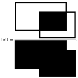
For the remaining predictions, an IoU threshold TNMS is specified to filter out redundant, highly overlapping predictions with relatively low confidences based on their bounding box positions through NMS, which is usually class-specific instead of class-agnostic. Traditional greedy NMS first sorts the predictions belonging to the same class in descending order based on their confidences, and then iterates through them following the same procedure as described below. It uses the top prediction as the base prediction to keep, and then computes the IoU between the base prediction and the remaining predictions, which all have lower confidences than the base prediction. IoU between two bounding box predictions is defined as the ratio between the area of overlap and the area of union, as illustrated by Equation (1):
![Ai 06 00141 i001]() When a prediction has an IoU larger than TNMS with the base prediction, it is removed. After NMS completes one iteration over the entire list, it moves on to the second top prediction and uses that as the new base prediction. This process is repeated until all the prediction lists of all the classes are iterated through [9].
When a prediction has an IoU larger than TNMS with the base prediction, it is removed. After NMS completes one iteration over the entire list, it moves on to the second top prediction and uses that as the new base prediction. This process is repeated until all the prediction lists of all the classes are iterated through [9].
2.7. TP and FP Identification
In image i, assuming Pi,j valid predictions are left for class j after confidence and NMS filtering, and Ai,j annotations exist for class j, the predictions are classified as either TP or FP based on a specified IoU threshold TTFP, which is typically no less than 50%. As the prediction and annotation bounding boxes should form unique one-to-one matching relationships, where each prediction is matched with at most one annotation, and each annotation is matched with at most one prediction, the IoUs between all predictions and annotations are exhaustively calculated, producing Pi,j × Ai,j prediction–annotation pairs. The pairs with IoUs below TTFP are removed. The remaining pairs are sorted in descending order of IoU, and filtered in two stages, by retaining only the first occurrence of each unique prediction and annotation, respectively. Finally, the predictions with matched annotations are classified as TPs, while the unmatched predictions are classified as FPs [10]. It is important to clarify that, for the purpose of constructing PR curves, FNs do not need to be explicitly identified, unlike when precision and recall are used as standalone metrics for evaluating object detector’s overall performance.
2.8. PR Curve Construction
After the TPs and FPs of all C classes in all N DTest images are identified, predictions across all images are pooled into C groups based on their classes, and each group is further utilized to construct a PR curve for the corresponding class. According to The PASCAL Visual Object Classes (VOC) Challenge by Everingham et al. [2], “For a given task and class, the precision/recall curve is computed from a method’s ranked output. Recall is defined as the proportion of all positive examples ranked above a given rank. Precision is the proportion of all examples above that rank which are from the positive class.” Assuming there are in total Pj valid predictions, TPj TP predictions, and Aj annotations for class j, the predictions are first sorted in descending order based on their confidences, and Pj pairs of precision and recall values are calculated at each prediction confidence rank, as illustrated by Table 1. Under the context of constructing PR curves, for a given ranked prediction, precision is calculated as cumulative TP over prediction rank, while recall is calculated as cumulative TP over total annotation Aj.
After calculating the precision and recall values at all prediction confidence ranks, the PR curve is constructed by plotting all precision–recall pairs, with the x-axis representing recall, and the y-axis representing precision.
2.9. AP Calculation
Raw PR curves often have a zigzag appearance (Figure 1), since precision can fluctuate with prediction confidence rank while recall consistently increases. While the concept of AP is meant to simply represent the AUC of a PR curve, the calculation of AP typically involves interpolation operations to stabilize and smooth the curve, and the AUC approximation methods vary depending on the interpolation techniques used. Below are four notable implementations of AP calculation in current literature.
2.9.1. 11-Point Interpolation
11-point interpolation was introduced by Everingham et al. in 2007 for the PASCAL Visual Object Classes Challenge 2007 (VOC2007) [11], and was officially documented in [2]. It approximates the area under a PR curve by averaging precisions at 11 recall levels, from 0 to 1 in steps of 0.1. The precision at each point is interpolated as the maximum precision observed at any recall greater than or equal to that point’s recall level. If no such point exists beyond a given recall level, the interpolated precision is assumed to be 0. For clarification, 11-point interpolation does not compute true AUC. Rather, it simplifies the AUC calculation by averaging a fixed set of interpolated precisions (Figure 1). The official code implementation can be found at [12]. Mathematically, 11-point interpolation is expressed as:
where,
2.9.2. All-Point Interpolation
All-point interpolation was introduced by Everingham et al. in 2010 for the PASCAL Visual Object Classes Challenge 2010 (VOC2010) [13], though it was never formally documented in a publication. It approximates the area under a PR curve as the right Riemann sum over all available points. The precision at each point is interpolated as the maximum precision observed at any recall greater than or equal to that point’s recall level, with sentinel points including (0,0) and (1,0) appended to the PR curve. For clarification, all-point interpolation does compute AUC based on step-wise interpolated PR curve (Figure 1). The official code implementation can be found at [14]. Mathematically, all-point interpolation is expressed as:
where,
and n ranges from 1 to Pj + 1 for class j due to the two appended sentinel points.
2.9.3. 101-Point Interpolation
101-point interpolation was introduced by Lin et al. in 2014 for the Microsoft COCO dataset [15], though it was never formally documented in a publication. It is very similar to the 11-point interpolation in nature, by approximating the area under a PR curve by averaging precisions at 101 recall levels, from 0 to 1 in steps of 0.01. The precision at each point is interpolated as the maximum precision observed at any recall greater than or equal to that point’s recall level. If no such point exists beyond a given recall level, the interpolated precision is assumed to be 0. For clarification, 101-point interpolation does not compute true AUC. Rather, it simplifies the AUC calculation by averaging a fixed set of interpolated precisions, and is more precise than 11-point interpolation (Figure 1). The official code implementation can be found at [16]. Mathematically, 101-point interpolation is expressed as:
where,
2.9.4. 101-Point Trapezoidal Interpolation
101-point trapezoidal interpolation, as implemented in the popular Ultralytics Python library, has not been formally documented in a publication. The name for this interpolation method is introduced in this article to distinguish it from existing methods while maintaining consistent naming conventions. Ultralytics’s default PR curve interpolation method, which is hard-coded and not user-configurable despite two interpolation options being present in the codebase, attempts to replicate the 101-point interpolation approach but deviates from the original definition in implementation. It approximates the area under a PR curve by summing 100 trapezoids formed by 101 points at recall levels from 0 to 1 in steps of 0.01. This method applies double interpolation. First, sentinel points (0,1) and (1,0) are appended to the PR curve. These differ slightly from the sentinel points used in all-point interpolation, but they do not materially affect the final AUC after interpolation. Second, all-point interpolation is applied to enforce a non-increasing PR curve. Finally, linear interpolation is performed at the fixed recall intervals to obtain the precision values used in the trapezoidal AUC calculation. For clarification, 101-point trapezoidal interpolation does compute AUC based on linearly interpolated PR curve, and typically yields results that more closely approximate the true AUC than the original all-point interpolation method (Figure 1). The official code implementation can be found at [17]. Mathematically, 101-point trapezoidal interpolation is expressed as:
where,
and n ranges from 1 to Pj + 1 for class j due to the two appended sentinel points.
2.10. mAP Calculation
To calculate mAP50–95, which is also variably denoted in literature as mAP@50–95, mAP@0.5–0.95, mAP@[0.5, 0.95], mAP50…95, etc., and often confusingly referred to simply as AP in studies involving the COCO dataset [18], a total of 10 × C APs for the C classes at 10 TTFP thresholds ranging from 0.5 to 0.95 with a step of 0.05 need to be calculated and then averaged. Mathematically:
where,
2.11. GFLOPs Counting
Commonly, only multiplication and addition operations in network layers are counted toward the total FLOPs of object detectors. From an implementation perspective, multiply–accumulate (MAC) operations are typically measured first, and FLOPs are subsequently calculated from them. Mathematically, for a single image forward pass:
where,
Using Ultralytics’s modified THOP library [19] as an example, by default, the following layers are included in the MAC count [20]:
- torch.nn.AdaptiveAvgPool1d;
- torch.nn.AdaptiveAvgPool2d;
- torch.nn.AdaptiveAvgPool3d;
- torch.nn.AvgPool1d;
- torch.nn.AvgPool2d;
- torch.nn.AvgPool3d;
- torch.nn.BatchNorm1d;
- torch.nn.BatchNorm2d;
- torch.nn.BatchNorm3d;
- torch.nn.Conv1d;
- torch.nn.Conv2d;
- torch.nn.Conv3d;
- torch.nn.ConvTranspose1d;
- torch.nn.ConvTranspose2d;
- torch.nn.ConvTranspose3d;
- torch.nn.GRU;
- torch.nn.GRUCell;
- torch.nn.InstanceNorm1d;
- torch.nn.InstanceNorm2d;
- torch.nn.InstanceNorm3d;
- torch.nn.LayerNorm;
- torch.nn.LeakyReLU;
- torch.nn.Linear;
- torch.nn.LSTM;
- torch.nn.LSTMCell;
- torch.nn.PReLU;
- torch.nn.RNN;
- torch.nn.RNNCell;
- torch.nn.Softmax;
- torch.nn.SyncBatchNorm;
- torch.nn.Upsample;
- torch.nn.UpsamplingBilinear2d;
- torch.nn.UpsamplingNearest2d.
The following layers, along with any others not explicitly listed, are ignored [20]:
- torch.nn.AdaptiveMaxPool1d;
- torch.nn.AdaptiveMaxPool2d;
- torch.nn.AdaptiveMaxPool3d;
- torch.nn.Dropout;
- torch.nn.MaxPool1d;
- torch.nn.MaxPool2d;
- torch.nn.MaxPool3d;
- torch.nn.PixelShuffle;
- torch.nn.ReLU;
- torch.nn.ReLU6;
- torch.nn.Sequential;
- torch.nn.ZeroPad2d.
2.12. ODEI Calculation
ODEI is mathematically expressed as:
A higher ODEI value indicates a more efficient object detector. Note, mAP50–95 should be expressed as a percentage, which ensures that the resulting ODEI values typically fall within a more interpretable range, such as tenths to single-digit integers, rather than extremely small decimal values with many digits.
2.13. Mandatory Parameter Declaration
For fair and transparent benchmarking of object detectors, ODEIs are only comparable when calculated under identical environment setups and evaluation configurations. To avoid ambiguity or future misinterpretation of reported ODEI values, this article, as the originator of the ODEI metric, proposes that the following seven parameters must be explicitly declared whenever an ODEI is invoked:
- Dataset name: name of the benchmarking dataset, which must be open-source and publicly accessible. Examples from the FiftyOne Dataset Zoo [21] include VOC-2007, VOC-2012, COCO-2014, COCO-2017, etc.
- Dataset split: portion of the dataset used for benchmarking. Common options include Train, Validation, Test, and Full, where Full means the entire dataset is used.
- Weight format: model weight file format. Examples include PyTorch, TensorFlow, TensorFlow Lite, TensorRT, ONNX, etc.
- Image size: model input image resolution. Examples include 320 representing 320 × 320, 480 representing 480 × 480, 640 representing 640 × 640, etc.
- Confidence threshold: minimum confidence score used to filter low-confidence predictions during postprocessing. Values range from 0 to 1.
- IoU threshold: maximum IoU allowed during NMS to filter overlapping predictions. Values range from 0 to 1. Use NA when NMS is not applicable to a model.
- Interpolation method: PR curve interpolation method for AP calculation as described in Section 2.9. Examples include 11-point, All-point, 101-point, 101-point trapezoidal, etc.
This list is intended to capture key benchmarking aspects that often vary across studies and to provide a standardized summary of the evaluation setup. Dataset is the foundation of any benchmarking activity and defines the task itself. Model weight format can affect GFLOPs depending on backend optimizations. Image input size determines the richness of raw pixel data and directly affects both detection accuracy and computational cost. Confidence threshold influences which predictions are retained for evaluation, and typically varies between lightweight and heavyweight models for the same detection tasks. NMS IoU threshold is tied to the object spatial density of the dataset, as higher thresholds may suit densely packed scenes, while lower ones are preferable for sparse layouts. PR curve interpolation method directly impacts the granularity of AP calculation, especially under lower confidence regimes. The list may evolve with future developments in object detection. For instance, certain state-of-the-art (SOTA) models such as DETR do not use NMS, making that parameter inapplicable. When necessary, an updated list of required parameters will be proposed and published accordingly. When calculating ODEIs for published studies, use NR as a placeholder for any parameters that are not explicitly reported. Table 2 provides a concise reference for the seven mandatory ODEI parameters abbreviated.
3. Example Metric Usage
This section demonstrates the application of ODEI using two SOTA object detection studies: YOLOv12 [22] and RT-DETRv3 [23]. YOLOv12 is an attention-centric detector and the latest addition to the YOLO family. It introduces the area attention module (A2) for efficient large receptive fields with reduced attention cost, residual efficient layer aggregation networks (R-ELAN) for stable optimization in large models, and architectural refinements such as FlashAttention integration, simplified attention design, adjusted multi-layer perceptron (MLP) ratios, and convolution-heavy blocks for better speed and memory efficiency. RT-DETRv3, on the other hand, is a training-optimized detector and the newest member of the RT-DETR family. It introduces a convolutional neural network (CNN)-based auxiliary head for dense supervision, a self-attention perturbation strategy to diversify label assignment across query groups, and a shared-weight decoder branch to improve query-ground truth matching, all implemented as training-only modules.
3.1. YOLOv12
The first two columns of Table 3 reproduce data from Table 1 in the article YOLOv12: Attention-Centric Real-Time Object Detectors by Tian et al. [22], published in 2025. Most mandatory parameters required for ODEI were not explicitly stated in the paper, and are therefore marked as NR in the table title. However, reasonable assumptions can be made based on contextual information. The authors specified, “We validate the proposed method on the MSCOCO 2017 dataset”, which implies the Validation split of the COCO-2017 dataset was likely used. They also noted, “The latencies of all models are tested on a T4 GPU with TensorRT FP16”, suggesting that the TensorRT format was likely also used when reporting GFLOPs. The title of Table 1 in the original article explicitly states, “All results are obtained using 640 × 640 inputs”, confirming an image input size of 640. Confidence and IoU thresholds were not disclosed in the paper. The authors stated they “report the standard mean average precision (mAP) on different object scales and IoU thresholds”, which implies the use of a 101-point-style interpolation method for the COCO dataset, while the references to the Ultralytics GitHub repository suggest the likely use of the 101-point trapezoidal interpolation method.
Based on the results in Table 3, YOLOv12-X is the most accurate object detector, achieving a 55.2% mAP50–95. YOLOv11-N and YOLOv12-N are the lightest models, each with a total of 6.5 GFLOPs. Among all models, YOLOv12-N demonstrates the highest efficiency, reaching an ODEI of 6.25. In the original publication, the authors grouped the evaluated detectors into five categories based on model size: N-scale, S-scale, M-scale, L-scale, and X-scale. As illustrated in Figure 2, model efficiency generally decreases as model size increases, despite larger models tending to achieve higher accuracy. In addition, newer YOLO versions are generally more efficient than their predecessors. In comparison, RT-DETR models exhibit significantly lower efficiency than their YOLO counterparts, particularly at the smaller model scales.
Figure 3 shows scatter plots of the mAP50–95 and GFLOPs values against their corresponding ODEI values from Table 3. It can be observed that mAP50–95 is generally negatively correlated with ODEI, which may seem counterintuitive since a higher mAP would be expected to result in a higher ODEI when GFLOPs remain constant. For the larger, more accurate models, their ODEI values are clustered closely together, indicating little differentiation in efficiency. In contrast, the lighter and less accurate models exhibit a more dispersed distribution, suggesting greater variation in efficiency among the smaller models. Interestingly, GFLOPs and ODEI follow a near-perfect hyperbolic decay relationship, where increasing computational complexity leads to an exponential decrease in efficiency.
3.2. RT-DETRv3
The first two columns of Table 4 reproduce data from Table 2 in the article RT-DETRv3: Real-time End-to-End Object Detection with Hierarchical Dense Positive Supervision by Wang et al. [23], published in 2024. Most mandatory parameters required for ODEI were not explicitly stated in the paper, and are therefore marked as NR in the table title. However, reasonable assumptions can be made based on contextual information. The title of Table 2 in the original article explicitly states “COCO val2017”, confirming the Validation split of the COCO-2017 dataset was used. The authors noted, “the latencies of all models are tested on T4 GPU with TensorRT FP16”, suggesting that the TensorRT format was likely also used when reporting GFLOPs. Model input image size, confidence thresholds, and IoU thresholds for the compared YOLO models were not disclosed in the paper. Regarding the PR curve interpolation method, the authors stated that “We adopted the same evaluation metric, AP, as used in the RT-DETR approach”, while the original RT-DETR publication [24] mentioned “We report the standard COCO metrics”, implying the use of a 101-point-style interpolation method.
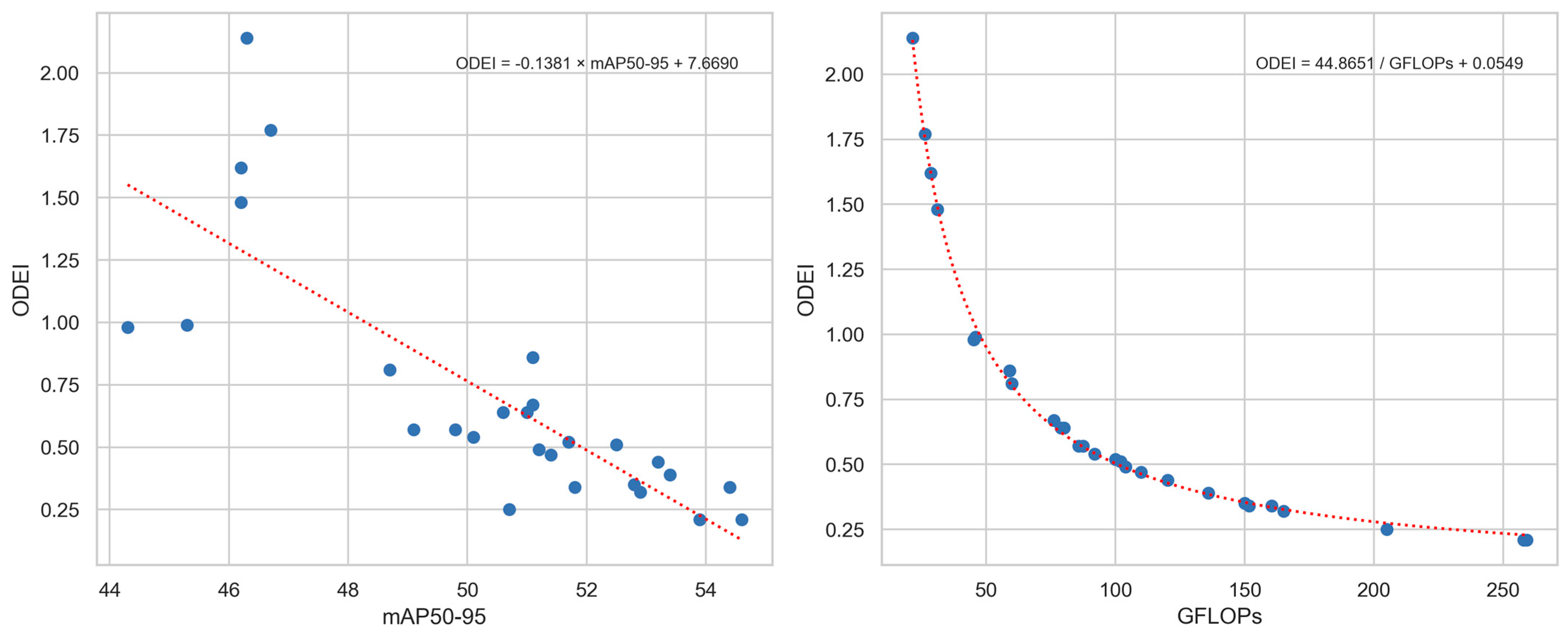
Based on the results in Table 4, RT-DETRv3-R101 is the most accurate object detector, achieving a 54.6% mAP50–95. YOLOV10-S is the lightest model, with a total of 21.6 GFLOPs. Among all models, YOLOV10-S demonstrates the highest efficiency, reaching an ODEI of 2.14. In the original publication, the authors grouped the evaluated detectors into four categories based on model size: S-scale, M-scale, L-scale, and X-scale. The ODEI distributions and trends are illustrated in Figure 4, while Figure 5 shows scatter plots of the mAP50–95 and GFLOPs values against their corresponding ODEI values. Both figures follow the same patterns observed in Figure 2 and Figure 3, and are therefore not redundantly described here.
4. Discussion
As deep learning continues to gain traction in academic research, object detectors are being increasingly applied across a wide range of disciplines. However, many application-oriented studies lack a fundamental understanding of object detector evaluation, and fail to thoroughly document their experimental setups. This to a large degree is due to the widespread use of open-source, user-friendly evaluation tools and application programming interfaces (APIs), which require minimal input but differ in default parameters and internal implementations. For example, the author’s prior work has utilized YOLOv4 [25,26,27], YOLOv7 [26], YOLOv8 [28], and YOLO11 [29] in different default configurations. YOLOv4 uses a default input image size of 608 × 608 [30], confidence threshold of 0.25 [31], IoU threshold of 0.45 [31], and all-point interpolation [31]. YOLOv7 uses a default input image size of 640 × 640 [32], confidence threshold of 0.001 [32], IoU threshold of 0.65 [32], and 101-point trapezoidal interpolation [33]. YOLOv8 and YOLO11 use a default input image size of 640 × 640 [34], confidence threshold of 0.001 [10], IoU threshold of 0.7 [34], and 101-point trapezoidal interpolation [17].
The incomprehensive documentation issue is exemplified in the YOLOv12 and RT-DETRv3 studies, as shown in the titles of Table 3 and Table 4. Both demonstrate this common shortcoming in modern object detection literature. While some missing details can be inferred from context, scientific research should aim for clarity and replicability. Any ambiguity, such as omitting the confidence threshold or the PR curve interpolation method, prevents fair and direct model comparison across studies, even if such parameters have a minor effect on results. Due to these inconsistencies, researchers often resort to isolated benchmarking within their own studies. While high-profile papers introducing SOTA models such as YOLOv12 and RT-DETRv3 generally use large public benchmark datasets and offer somewhat better documentation, many papers claiming SOTA detector performance use private datasets with vague or incomplete setup descriptions.
To address these issues, this article proposes a set of mandatory parameters that must be reported when invoking ODEI. The goal is to standardize object detector evaluation practices and enable reliable cross-study model comparisons. By requiring detailed reporting and promoting a universal efficiency index, ODEI helps bridge the gap between disparate studies and fosters a more coherent benchmarking ecosystem.
Hardware inconsistency is another common limitation that hinders cross-study compatibility of object detector evaluation results. The primary reason GFLOPs are used in ODEI instead of time-based metrics such as inference time is to eliminate hardware dependency, thereby enabling consistent and reproducible evaluations across different studies. While time-based metrics more accurately reflect real-world inference speed, they are heavily influenced by hardware configurations and runtime environments. In contrast, GFLOPs provide a hardware-agnostic, purely software-based measure, which, while less representative of practical deployment speed, ensures comparability. This tradeoff can be viewed as a limitation of ODEI. Nevertheless, since GFLOPs and inference time are typically highly correlated, GFLOPs remain a reliable proxy for measuring model computational efficiency.
In both the YOLOv12 and RT-DETRv3 studies, ODEI effectively identified the most efficient or best-balanced object detectors. The results suggest that the computational cost of improving detector accuracy is currently too high: slight gains in mAP50–95 require disproportionately large increases in GFLOPs, resulting in significantly lower ODEIs for larger-scale models compared to their lighter counterparts. For future research aimed at developing efficient object detectors, prioritizing lightweight models that maintain reasonable accuracy may be more promising than chasing marginal accuracy improvements through heavier architectures.
The current landscape of object detector benchmarking is fragmented and inconsistently maintained. Platforms such as Papers With Code [35], Hugging Face [36], Roboflow [37], COCO [38], etc., each provide their own leaderboards, often covering different datasets and model subsets. Notably, SOTA models such as YOLOv12 and RT-DETRv3 are not always included. While mAP50–95 remains the dominant metric on these leaderboards, model computational complexity is rarely accounted for. ODEI has the potential to supplement, or even replace, mAP50–95 as a more comprehensive efficiency metric, providing a balanced view of both accuracy and speed. In doing so, it could serve as a new gold standard for guiding future object detection research and industrial benchmarking.
5. Conclusions
ODEI, defined with seven mandatory parameters, is designed as a universal metric for evaluating object detector efficiency and promoting fair, transparent benchmarking in research. However, the list of mandatory parameters may require updates in response to future trends in object detection. The author intends to take the initiative in establishing an object detector leaderboard using ODEI and AriAplBud [28] in a forthcoming publication.
Funding
This research received no external funding.
Institutional Review Board Statement
Not applicable.
Informed Consent Statement
Not applicable.
Data Availability Statement
The original contributions presented in this study are included in the article. Further inquiries can be directed to the corresponding author.
Conflicts of Interest
The author declare no conflicts of interest.
References
- Goutte, C.; Gaussier, E. A Probabilistic Interpretation of Precision, Recall and f-Score. In Advances in Information Retrieval; Springer: Berlin/Heidelberg, Germany, 2005; pp. 345–359. [Google Scholar] [CrossRef]
- Everingham, M.; Van Gool, L.; Williams, C.K.I.; Winn, J.; Zisserman, A. The Pascal Visual Object Classes (VOC) Challenge. Int. J. Comput. Vis. 2010, 88, 303–338. [Google Scholar] [CrossRef]
- Ríos, J.O. Dynamically Adapting Floating-Point Precision to Accelerate Deep Neural Network Training. 2023. Available online: https://upcommons.upc.edu/bitstream/handle/2117/404063/TJHOR1de1.pdf?sequence=1&isAllowed=y (accessed on 24 June 2025).
- Suhaimi, N.S.; Othman, Z.; Yaakub, M.R. Comparative Analysis Between Macro and Micro-Accuracy in Imbalance Dataset for Movie Review Classification. In Proceedings of the Seventh International Congress on Information and Communication Technology, London, UK, 21–24 February 2022; pp. 83–93. [Google Scholar]
- Takahashi, K.; Yamamoto, K.; Kuchiba, A.; Koyama, T. Confidence Interval for Micro-Averaged F 1 and Macro-Averaged F 1 Scores. Appl. Intell. 2022, 52, 4961–4972. [Google Scholar] [CrossRef] [PubMed]
- Oh, S.; Kwon, Y.; Lee, J. Optimizing Real-Time Object Detection in a Multi-Neural Processing Unit System. Sensors 2025, 25, 1376. [Google Scholar] [CrossRef] [PubMed]
- Ryu, J.; Kim, H. Adaptive Object Detection: Balancing Accuracy and Inference Time. In Proceedings of the 2023 IEEE International Conference on Consumer Electronics-Asia (ICCE-Asia), Busan, Republic of Korea, 23–25 October 2023. [Google Scholar]
- Ultralytics/Ultralytics/Nn/Modules/Head.Py. Available online: https://github.com/ultralytics/ultralytics/blob/main/ultralytics/nn/modules/head.py (accessed on 24 June 2025).
- Ultralytics/Ultralytics/Utils/Ops.Py. Available online: https://github.com/ultralytics/ultralytics/blob/main/ultralytics/utils/ops.py (accessed on 24 June 2025).
- Ultralytics/Ultralytics/Engine/Validator.Py. Available online: https://github.com/ultralytics/ultralytics/blob/main/ultralytics/engine/validator.py (accessed on 24 June 2025).
- Everingham, M.; Van Gool, L.; Williams, C.K.I.; Winn, J.; Zisserman, A. The PASCAL Visual Object Classes Challenge 2007. Available online: http://host.robots.ox.ac.uk/pascal/VOC/voc2007/index.html (accessed on 24 June 2025).
- Everingham, M.; Van Gool, L.; Williams, C.K.I.; Winn, J.; Zisserman, A. VOCdevkit_08-Jun-2007.Tar. Available online: http://host.robots.ox.ac.uk/pascal/VOC/voc2007/VOCdevkit_08-Jun-2007.tar (accessed on 24 June 2025).
- Everingham, M.; Van Gool, L.; Williams, C.K.I.; Winn, J.; Zisserman, A. Visual Object Classes Challenge 2010 (VOC2010). Available online: http://host.robots.ox.ac.uk/pascal/VOC/voc2010/index.html (accessed on 24 June 2025).
- Everingham, M.; Van Gool, L.; Williams, C.K.I.; Winn, J.; Zisserman, A. VOCdevkit_08-May-2010.Tar. Available online: http://host.robots.ox.ac.uk/pascal/VOC/voc2010/VOCdevkit_08-May-2010.tar (accessed on 24 June 2025).
- Lin, T.-Y.; Maire, M.; Belongie, S.; Bourdev, L.; Girshick, R.; Hays, J.; Perona, P.; Ramanan, D.; Zitnick, C.L.; Dollár, P. Microsoft COCO: Common Objects in Context. In Proceedings of the 13th European Conference on Computer Vision (ECCV), Zurich, Switzerland, 6–12 September 2014; pp. 740–755. [Google Scholar]
- Cocoapi/PythonAPI/Pycocotools/Cocoeval.Py. Available online: https://github.com/cocodataset/cocoapi/blob/master/PythonAPI/pycocotools/cocoeval.py (accessed on 24 June 2025).
- Ultralytics/Ultralytics/Utils/Metrics.Py. Available online: https://github.com/ultralytics/ultralytics/blob/main/ultralytics/utils/metrics.py (accessed on 24 June 2025).
- Detection Evaluation. Available online: https://cocodataset.org/#detection-eval (accessed on 24 June 2025).
- THOP: PyTorch-OpCounter. Available online: https://github.com/ultralytics/thop/tree/main (accessed on 24 June 2025).
- Thop/Thop/Profile.Py. Available online: https://github.com/ultralytics/thop/blob/main/thop/profile.py (accessed on 24 June 2025).
- FiftyOne Dataset Zoo. Available online: https://docs.voxel51.com/dataset_zoo/index.html (accessed on 24 June 2025).
- Tian, Y.; Ye, Q.; Doermann, D. YOLOv12: Attention-Centric Real-Time Object Detectors. arXiv 2025, arXiv:2502.12524. [Google Scholar]
- Wang, S.; Xia, C.; Lv, F.; Shi, Y. RT-DETRv3: Real-Time End-to-End Object Detection with Hierarchical Dense Positive Supervision. arXiv 2024, arXiv:2409.08475. [Google Scholar]
- Zhao, Y.; Lv, W.; Xu, S.; Wei, J.; Wang, G.; Dang, Q.; Liu, Y.; Chen, J. DETRs Beat YOLOs on Real-Time Object Detection. In Proceedings of the 2024 IEEE/CVF Conference on Computer Vision and Pattern Recognition (CVPR), Seattle, WA, USA, 16–22 June 2024. [Google Scholar] [CrossRef]
- Yuan, W.; Choi, D. UAV-Based Heating Requirement Determination for Frost Management in Apple Orchard. Remote Sens. 2021, 13, 273. [Google Scholar] [CrossRef]
- Yuan, W. Accuracy Comparison of YOLOv7 and YOLOv4 Regarding Image Annotation Quality for Apple Flower Bud Classification. AgriEngineering 2023, 5, 413–424. [Google Scholar] [CrossRef]
- Yuan, W.; Choi, D.; Bolkas, D.; Heinemann, P.H.; He, L. Sensitivity Examination of YOLOv4 Regarding Test Image Distortion and Training Dataset Attribute for Apple Flower Bud Classification. Int. J. Remote Sens. 2022, 43, 3106–3130. [Google Scholar] [CrossRef]
- Yuan, W. AriAplBud: An Aerial Multi-Growth Stage Apple Flower Bud Dataset for Agricultural Object Detection Benchmarking. Data 2024, 9, 36. [Google Scholar] [CrossRef]
- Yuan, W.; Li, P. Lightweight GAN-Assisted Class Imbalance Mitigation for Apple Flower Bud Detection. Big Data Cogn. Comput. 2025, 9, 28. [Google Scholar] [CrossRef]
- Darknet/Cfg/Yolov4.Cfg. Available online: https://github.com/AlexeyAB/darknet/blob/master/cfg/yolov4.cfg (accessed on 24 June 2025).
- Darknet/Src/Detector.C. Available online: https://github.com/AlexeyAB/darknet/blob/master/src/detector.c (accessed on 24 June 2025).
- Yolov7/Test.Py. Available online: https://github.com/WongKinYiu/yolov7/blob/main/test.py (accessed on 24 June 2025).
- Yolov7/Utils/Metrics.Py. Available online: https://github.com/WongKinYiu/yolov7/blob/main/utils/metrics.py (accessed on 24 June 2025).
- Ultralytics/Ultralytics/Cfg/Default.Yaml. Available online: https://github.com/ultralytics/ultralytics/blob/main/ultralytics/cfg/default.yaml (accessed on 24 June 2025).
- Object Detection. Available online: https://paperswithcode.com/task/object-detection (accessed on 24 June 2025).
- Object Detection Leaderboard. Available online: https://huggingface.co/spaces/hf-vision/object_detection_leaderboard (accessed on 24 June 2025).
- Computer Vision Model Leaderboard. Available online: https://leaderboard.roboflow.com/ (accessed on 24 June 2025).
- Detection Leaderboard. Available online: https://cocodataset.org/#detection-leaderboard (accessed on 24 June 2025).
Figure 1.
Sample raw PR curve and corresponding interpolation results of four different methods.
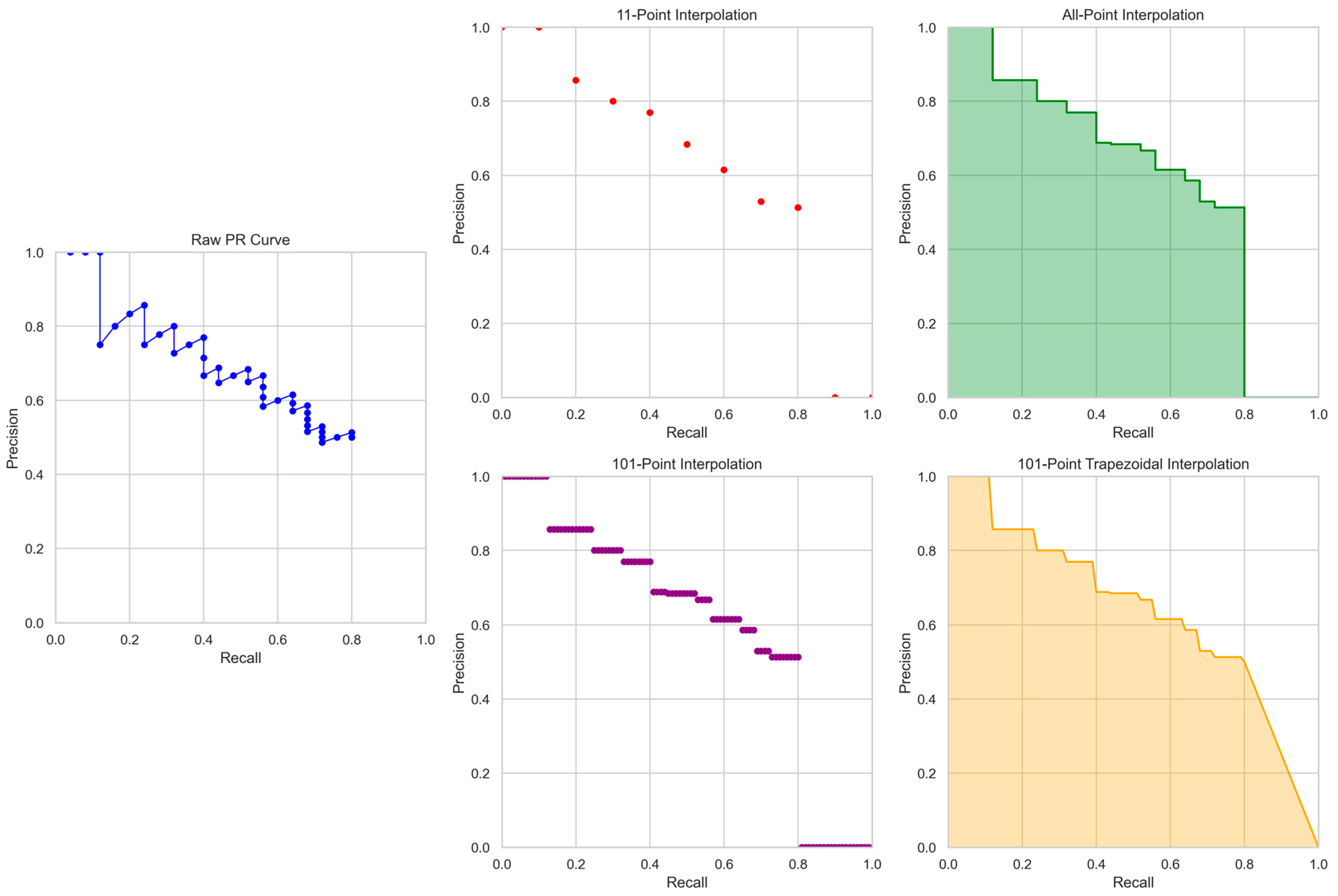
Figure 2.
Box and line plots showing ODEI distributions by model scale and ODEI trends by object detector in the YOLOv12 study.
Figure 2.
Box and line plots showing ODEI distributions by model scale and ODEI trends by object detector in the YOLOv12 study.
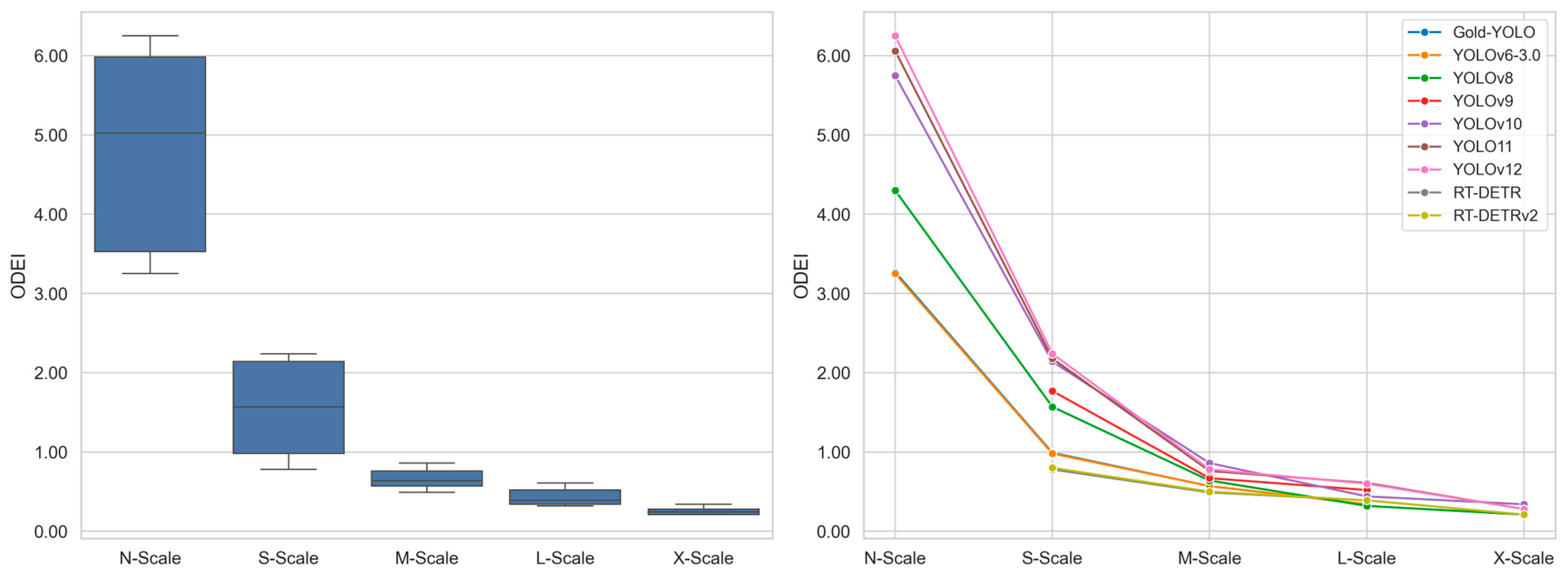
Figure 3.
Scatter plots of mAP50–95, GFLOPs, and ODEI values from the YOLOv12 study.
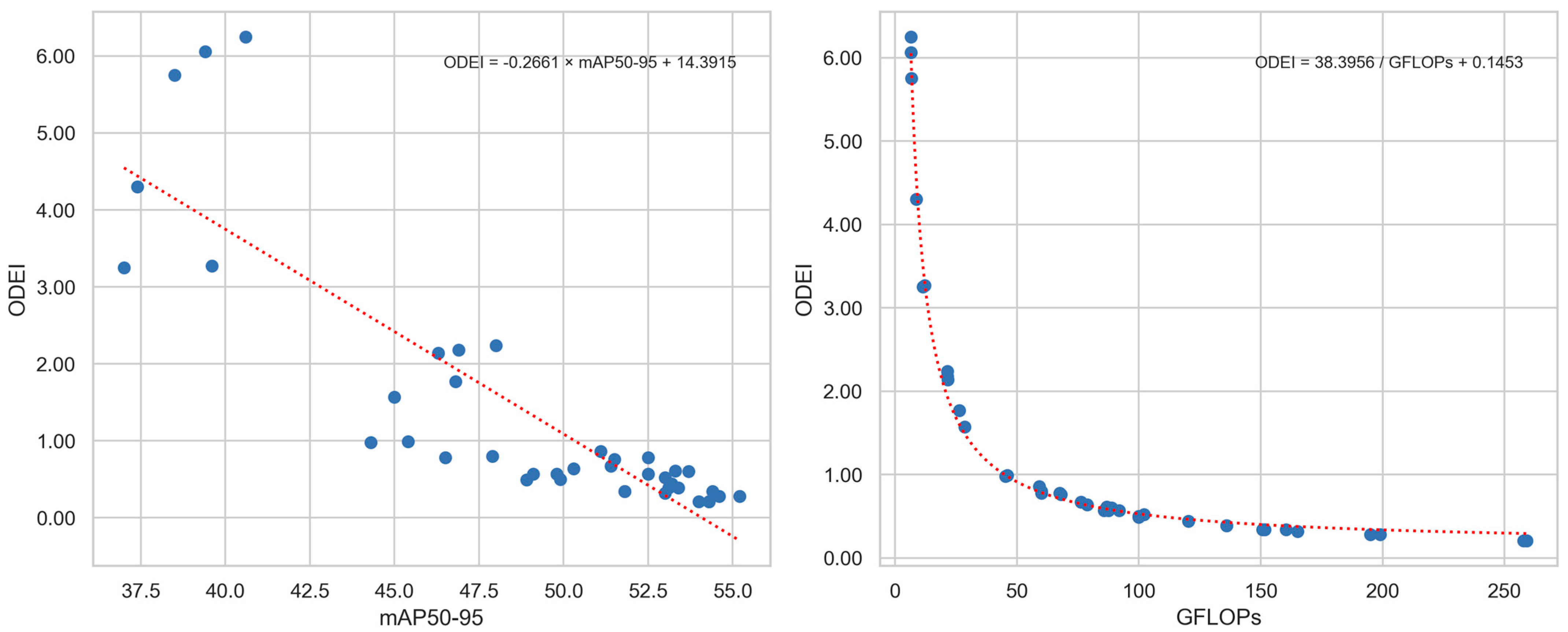
Figure 4.
Box and line plots showing ODEI distributions by model scale and ODEI trends by object detector in the RT-DETRv3 study.
Figure 4.
Box and line plots showing ODEI distributions by model scale and ODEI trends by object detector in the RT-DETRv3 study.
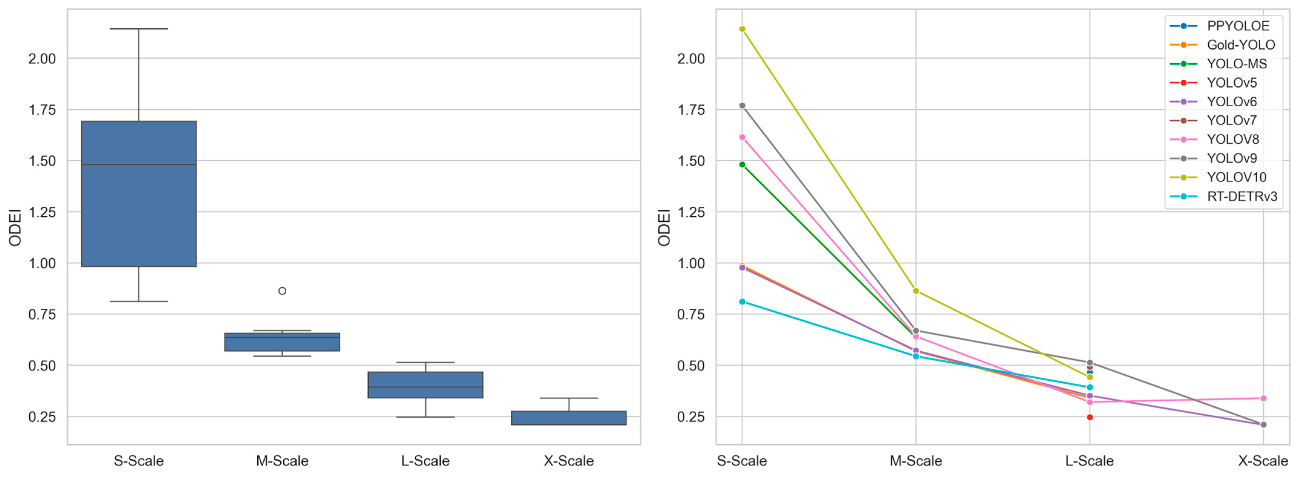
Figure 5.
Scatter plots of mAP50–95, GFLOPs, and ODEI values from the RT-DETRv3 study.

Table 1.
Illustration of precision and recall calculation for PR curve construction of class j in dataset DTest, assuming Pj total predictions, TPj total TP predictions, and Aj total annotations.
Table 1.
Illustration of precision and recall calculation for PR curve construction of class j in dataset DTest, assuming Pj total predictions, TPj total TP predictions, and Aj total annotations.
| Prediction Rank | Confidence | TP/FP | Cumulative TP | Precision | Recall |
|---|---|---|---|---|---|
| 1 | 0.99 | TP | 1 | 1/1 | 1/Aj |
| 2 | 0.98 | FP | 1 | 1/2 | 1/Aj |
| 3 | 0.92 | TP | 2 | 2/3 | 2/Aj |
| 4 | 0.91 | FP | 2 | 2/4 | 2/Aj |
| 5 | 0.85 | FP | 2 | 2/5 | 2/Aj |
| 6 | 0.83 | TP | 3 | 3/6 | 3/Aj |
| … | |||||
| Pj | 0.69 | TP | TPj | TPj/Pj | TPj/Aj |
Table 2.
ODEI mandatory parameter quick reference guide.
| Parameter | Description | Example |
|---|---|---|
| DN | Dataset name | VOC-2007, VOC-2012, COCO-2014, COCO-2017, NR |
| DS | Dataset split | Train, Validation, Test, Full, NR |
| WF | Model weight format | PyTorch, TensorFlow, TensorFlow Lite, TensorRT, ONNX, NR |
| IS | Image input size | 320, 480, 640, NR |
| CT | Confidence threshold | 0.001, 0.25, 0.5, NR |
| IT | NMS IoU threshold | 0.45, 0.65, 0.7, NA, NR |
| IM | PR curve interpolation method | 11-point, All-point, 101-point, 101-point trapezoidal, NR |
Table 3.
ODEIs of the compared object detectors in the YOLOv12 study @ (COCO-2017, NR, NR, 640, NR, NR/NA, NR).
Table 3.
ODEIs of the compared object detectors in the YOLOv12 study @ (COCO-2017, NR, NR, 640, NR, NR/NA, NR).
| Model | mAP50–95 | GFLOPs | ODEI |
|---|---|---|---|
| YOLOv6-3.0-N | 37.0 | 11.4 | 3.25 |
| Gold-YOLO-N | 39.6 | 12.1 | 3.27 |
| YOLOv8-N | 37.4 | 8.7 | 4.30 |
| YOLOv10-N | 38.5 | 6.7 | 5.75 |
| YOLO11-N | 39.4 | 6.5 | 6.06 |
| YOLOv12-N | 40.6 | 6.5 | 6.25 |
| YOLOv6-3.0-S | 44.3 | 45.3 | 0.98 |
| Gold-YOLO-S | 45.4 | 46.0 | 0.99 |
| YOLOv8-S | 45.0 | 28.6 | 1.57 |
| RT-DETR-R18 | 46.5 | 60.0 | 0.78 |
| RT-DETRv2-R18 | 47.9 | 60.0 | 0.80 |
| YOLOv9-S | 46.8 | 26.4 | 1.77 |
| YOLOv10-S | 46.3 | 21.6 | 2.14 |
| YOLO11-S | 46.9 | 21.5 | 2.18 |
| YOLOv12-S | 48.0 | 21.4 | 2.24 |
| YOLOv6-3.0-M | 49.1 | 85.8 | 0.57 |
| Gold-YOLO-M | 49.8 | 87.5 | 0.57 |
| YOLOv8-M | 50.3 | 78.9 | 0.64 |
| RT-DETR-R34 | 48.9 | 100.0 | 0.49 |
| RT-DETRv2-R34 | 49.9 | 100.0 | 0.50 |
| YOLOv9-M | 51.4 | 76.3 | 0.67 |
| YOLOv10-M | 51.1 | 59.1 | 0.86 |
| YOLO11-M | 51.5 | 68.0 | 0.76 |
| YOLOv12-M | 52.5 | 67.5 | 0.78 |
| YOLOv6-3.0-L | 51.8 | 150.7 | 0.34 |
| Gold-YOLO-L | 51.8 | 151.7 | 0.34 |
| YOLOv8-L | 53.0 | 165.2 | 0.32 |
| RT-DETR-R50 | 53.1 | 136.0 | 0.39 |
| RT-DETRv2-R50 | 53.4 | 136.0 | 0.39 |
| YOLOv9-C | 53.0 | 102.1 | 0.52 |
| YOLOv10-B | 52.5 | 92.0 | 0.57 |
| YOLOv10-L | 53.2 | 120.3 | 0.44 |
| YOLO11-L | 53.3 | 86.9 | 0.61 |
| YOLOv12-L | 53.7 | 88.9 | 0.60 |
| YOLOv8-X | 54.0 | 257.8 | 0.21 |
| RT-DETR-R101 | 54.3 | 259.0 | 0.21 |
| RT-DETRv2-R101 | 54.3 | 259.0 | 0.21 |
| YOLOv10-X | 54.4 | 160.4 | 0.34 |
| YOLO11-X | 54.6 | 194.9 | 0.28 |
| YOLOv12-X | 55.2 | 199.0 | 0.28 |
Table 4.
ODEIs of the compared object detectors in the RT-DETRv3 study @ (COCO-2017, Validation, NR, NR, NR, NR/NA, NR).
Table 4.
ODEIs of the compared object detectors in the RT-DETRv3 study @ (COCO-2017, Validation, NR, NR, NR, NR/NA, NR).
| Model | mAP50–95 | GFLOPs | ODEI |
|---|---|---|---|
| YOLOv6-3.0-S | 44.3 | 45.3 | 0.98 |
| Gold-YOLO-S | 45.4 | 46.0 | 0.99 |
| YOLO-MS-S | 46.2 | 31.2 | 1.48 |
| YOLOv8-S | 46.2 | 28.6 | 1.62 |
| YOLOv9-S | 46.7 | 26.4 | 1.77 |
| YOLOV10-S | 46.3 | 21.6 | 2.14 |
| RT-DETRv3-R18 | 48.7 | 60.0 | 0.81 |
| YOLOv6-3.0-M | 49.1 | 85.8 | 0.57 |
| Gold-YOLO-M | 49.8 | 87.5 | 0.57 |
| YOLO-MS | 51.0 | 80.2 | 0.64 |
| YOLOv8-M | 50.6 | 78.9 | 0.64 |
| YOLOv9-M | 51.1 | 76.3 | 0.67 |
| YOLOV10-M | 51.1 | 59.1 | 0.86 |
| RT-DETRv3-R34 | 50.1 | 92.0 | 0.54 |
| RT-DETRv3-R50m | 51.7 | 100.0 | 0.52 |
| Gold-YOLO-L | 51.8 | 151.7 | 0.34 |
| YOLOv5-X | 50.7 | 205.0 | 0.25 |
| PPYOLOE-L | 51.4 | 110.0 | 0.47 |
| YOLOv6-L | 52.8 | 150.0 | 0.35 |
| YOLOv7-L | 51.2 | 104.0 | 0.49 |
| YOLOV8-L | 52.9 | 165.0 | 0.32 |
| YOLOv9-C | 52.5 | 102.1 | 0.51 |
| YOLOV10-L | 53.2 | 120.3 | 0.44 |
| RT-DETRv3-R50 | 53.4 | 136.0 | 0.39 |
| YOLOv8-X | 53.9 | 257.8 | 0.21 |
| YOLOv10-X | 54.4 | 160.4 | 0.34 |
| RT-DETRv3-R101 | 54.6 | 259.0 | 0.21 |
Disclaimer/Publisher’s Note: The statements, opinions and data contained in all publications are solely those of the individual author(s) and contributor(s) and not of MDPI and/or the editor(s). MDPI and/or the editor(s) disclaim responsibility for any injury to people or property resulting from any ideas, methods, instructions or products referred to in the content. |
© 2025 by the author. Licensee MDPI, Basel, Switzerland. This article is an open access article distributed under the terms and conditions of the Creative Commons Attribution (CC BY) license (https://creativecommons.org/licenses/by/4.0/).
Share and Cite
MDPI and ACS Style
Yuan, W. ODEI: Object Detector Efficiency Index. AI 2025, 6, 141. https://doi.org/10.3390/ai6070141
AMA Style
Yuan W. ODEI: Object Detector Efficiency Index. AI. 2025; 6(7):141. https://doi.org/10.3390/ai6070141
Chicago/Turabian StyleYuan, Wenan. 2025. "ODEI: Object Detector Efficiency Index" AI 6, no. 7: 141. https://doi.org/10.3390/ai6070141
APA StyleYuan, W. (2025). ODEI: Object Detector Efficiency Index. AI, 6(7), 141. https://doi.org/10.3390/ai6070141