Fusing Horizon Information for Visual Localization

Abstract

Localization is the foundation and core of autonomous driving. Current visual localization methods rely heavily on high-definition maps. However, high-definition maps are not only costly but also have poor real-time performance. In autonomous driving, place recognition is equally crucial and of great significance. Existing place recognition methods are deficient in local feature extraction and position and orientation errors can occur during the matching process. To address these limitations, this paper presents a robust multi-dimensional feature fusion framework for place recognition. Unlike existing methods such as OrienterNet, which homogenously process images and maps at the underlying feature level while neglecting modal disparities, our framework—applied to existing 2D maps—introduces a heterogeneous structural-semantic approach inspired by OrienterNet. It employs structured Stixel features (containing positional information) to capture image geometry, while representing the OSM environment through polar coordinate-based building distributions. Dedicated encoders are designed to adapt to each modality. Additionally, global relational features are generated by computing distances and angles between the current position and building pixels in the map, providing the system with detailed spatial relationship information. Subsequently, individual Stixel features are rotationally matched with global relations to achieve feature matching at diverse angles. During the BEV map matching process in OrienterNet, visual localization relies primarily on horizontal image information. In contrast, the novel method proposed herein performs matching based on vertical image information while fusing horizontal cues to complete place recognition. Extensive experimental results demonstrate that the proposed method significantly outperforms the mentioned state-of-the-art approaches in localization accuracy, effectively resolving the existing limitations.

1. Introduction

The innovation of localization technologies has propelled the transformation of autonomous driving and travel modalities. There has been a continuous evolution from GPS to high-precision sensor positioning technologies. The Global Navigation Satellite System (GNSS) is capable of efficiently and precisely locating vehicles; however, achieving higher precision incurs greater costs and is readily subject to environmental disturbances. To reduce the dependence on GNSS and improve the positioning reliability in complex environments, positioning methods based on sensors such as vision and LiDAR [1] have been widely studied. Visual localization determines the location and orientation of the camera in the scene through the given query image, which has become a fundamental task in computer vision and robotics and is very important in automatic driving, robot navigation, augmented reality, and other scenes [2].

Sarlin et al. first proposed an end-to-end algorithm called OrienterNet [3], which estimates the location and orientation of the query image by matching the Bird’s-Eye View (BEV) with the OpenStreetMap (OSM), without a HD map [4]. Due to the advantages of OSM, such as global consistency, a lightweight map-building process, and a large amount of publicly available road information, Mu et al. used OSM information as the environmental representation for global planning during the global navigation process [5,6].

However, as shown in Figure 1, the traditional deep learning algorithm cannot effectively extract the deep information of the image in the process of feature extraction, the resolution of the deep feature is greatly reduced, some key details are lost, and the feature map shows a relatively large fuzzy area. In addition, the OrienterNet algorithm has the problem of position and orientation errors in the process of BEV and OSM map matching.

We propose a new algorithm to solve the above problems. In the process of feature extraction, the input image is deeply analyzed to extract the Stixel [7] feature, and the corresponding Stixel feature is extracted from the OSM. This not only enhances the feature representation ability but also makes the features more discriminative, which is beneficial for the subsequent matching process. Then, a partitioning method based on distance and angle is proposed. In the process of feature matching, according to different distances and angles, the matching process is divided into different intensity levels. The single rod pixel feature and the global relationship feature are rotated to achieve feature matching from different angles. The relationship between the image and the global feature is considered more meticulously, and the information contained in the distance and angle is fully used, so as to achieve more accurate and reliable matching effects.

2. Related Work

In autonomous driving, visual localization provides the position and attitude information of autonomous vehicles in the global environment, which is like establishing a “coordinate system” for the vehicles, enabling them to know where they are and in which direction they are heading. Traditional visual positioning may mainly establish a global reference system and determine the position and direction of the vehicle based on the feature comparison between the camera images and the map or model. However, it has deficiencies in the perception of local environmental details. As a result of the research, it was found that the Stixel representation can be utilized to focus on the perception of the local environment around the vehicle. By extracting features from camera images, it can identify road obstacles and obtain road feature information. It is a further refined analysis of the vehicle’s surrounding environment based on the global position determined by visual localization. It can be said that visual localization tells the vehicle “where I am”, while Stixel representation further answers “what is around me”, providing more specific environmental information for the vehicle’s safe driving and path planning, and complementing the deficiency of visual localization in terms of environmental details. Feature matching accurately determines the position coordinates of the vehicle by comparing the features in the sensor data with those in the map or model. It relies on the global position framework provided by visual localization and the local environmental features extracted by Stixel representation and is a further optimization and refinement of the vehicle’s position information. Feature matching uses the information provided by the former two and, through more meticulous feature comparison and matching algorithms, can more accurately determine the position of the vehicle in complex environments.

2.1. Visual Localization

Sarlin proposed OrienterNet [3], which estimates the pose of query images by matching the Bird’s-Eye View with the available maps in OpenStreetMap, achieving certain results in positioning based on lightweight navigation maps. Samano et al. [8] utilized low-dimensional embedding spaces to geolocate panoramic images on two-dimensional navigation maps [9]. Park et al. [10] significantly enhanced the model’s spatial recognition and structural understanding ability of lane lines by using BEV features [11]. However, the 2D projection of BEV based on the orthographic projection principle inevitably loses height information, rendering it unable to accurately identify multi-layered structures. Moreover, large nearby occluding objects create extensive blind areas, severing the transmission of spatial information and undermining the integrity of far-end features, Therefore, simply using the features of BEV images for matching will still result in certain directional errors, like OrienterNet [3]. He et al. proposed an end-to-end positioning network called EgoVM [12], which uses lightweight vectorized maps to achieve precise self-positioning instead of heavy point-based maps [13]. While it is true that in many cases vector maps are useful, in some scenarios vector maps have difficulty adapting to complex road conditions such as temporary buildings, lack the ability to adapt to the environment, and the semantic information of the maps fails to match the ever-changing scenarios. Wu et al. [14] adopted coarse-to-fine feature matching and hierarchical strategies to achieve sub-meter level positioning using only navigation maps, fusing surround-view images and navigation maps and aligning BEV and map features. Sarlin et al. [15] proposed a self-supervised neural map method for visual localization and semantic understanding. Through self-supervised learning, the model can automatically learn the feature representation of the environment without a large number of annotation data, so as to achieve accurate location estimation and in-depth understanding of scene semantics [16]. Zhao et al. proposed a visual localization framework, PNeRFLoc [2], that combines the neural radiance field with the visual localization task. By optimizing the parameters of the neural radiance field, the model can accurately estimate the localization and attitude of the camera in the scene according to the input image. Using the strong modeling ability of the neural radiance field, the positioning accuracy and robustness are improved. Recently, some methods have leveraged Transformer architectures to address localization problems. TransGeo [17], the first pure Transformer-based model for cross-view localization, employs attention-guided cropping to optimize the alignment between street-view and aerial images, achieving high accuracy but suffering from weak cross-domain generalization and heavy data dependency. In contrast, LoFTR [18] uses Transformer to enable detector-free dense feature matching, solving the challenge of feature matching in low-texture or occluded scenes, yet it shows limited adaptability to extreme scale variations or irregular viewpoints. LocNet [19] achieves efficient matching between LiDAR point clouds and static maps via Siamese networks, but it suffers from poor robustness in dynamic environments, sensitivity to environmental interference, and ambiguity in low-texture scenarios. TransFusion [20] achieves cross-modal spatial alignment between images and point clouds via Transformer self-attention, but it suffers from failure in sparse scenarios and insufficient semantic fusion.

2.2. Stixel Representation

In the complex scenarios of autonomous driving, extracting Stixel features from camera images is of great significance. It can efficiently identify various potential obstacles on the road, and the effect is even better when combined with a binocular vision system. It can acquire stereo information to assist in estimating depth and distance, improving the accuracy and reliability of obstacle detection and ensuring the safety of vehicles. In the process of road environment perception, dividing the road area into Stixels can extract key features such as the texture and color of the road, helping vehicles to recognize information such as lane markings and providing basic data for path planning and navigation. Moreover, Stixels show strong robustness in the face of complex situations such as illumination changes and partial occlusions.

On the one hand, as shown in Figure 1, the resolution of high-level features in traditional deep learning decreases, and key details are lost. However, the Stixel feature map can better handle depth, edge, and height information; distinguish regions through colors; and has relatively better expressiveness. On the other hand, compared with the static map information of OSM, the environmental information it can provide is relatively simple, while the Stixel representation can more comprehensively reflect the environmental features. Thus, the selection of Stixel features derived from both the input image and the OSM (OpenStreetMap) image not only strengthens the feature representation capability but also enhances the distinctiveness of these features for more effective matching.

Moreover, for the angular matching of Stixel features, it can more meticulously consider the relationship between the image and the global features. The angular feature matching has good perspective invariance and scale adaptability, performs better in handling distant objects and maintaining boundary details, effectively weakens the influence of local errors, and enhances the adaptability to occluded and sparse scenes.

2.3. Feature Matching in Place Recognition

Positioning technology provides a framework and range for place recognition. Before place recognition, it is necessary to know the approximate area in order to search for features. Feature matching determines the position coordinates by comparing the features in the sensor data with those in the known map or model. In autonomous driving, the real-time point cloud data [21] is matched with the high-precision map data. For example, the point cloud models of objects such as roads have been stored in the map. LiDAR distinguishes different objects according to the reflection intensity of laser signals. In addition to the geometric features, the reflection intensity features can also be used in the matching process. In the method we have proposed, the crucial step of feature extraction is first carried out [22]. Specifically, an in-depth analysis is conducted on the input image to extract the Stixel features therein. At the same time, the corresponding Stixel features are also extracted from the global data of OpenStreetMap (OSM). Subsequently, in the critical stage of rotational matching between a single image and the global features, we introduced a partitioning method based on distance and angle differences. According to different distance and angle situations, the matching process is divided into different intensity levels. In this way, the relationship between the image and the global features can be considered more meticulously, and the information contained in the distance and angle can be fully utilized, so as to achieve a more accurate and reliable matching effect.

3. Method

The visual localization method proposed in this paper effectively fuses multiple types of information to achieve precise positioning through four closely integrated modules. As illustrated in Figure 2, the framework incorporates two critical matching processes. First, the BEV-Map Matching module aligns the Neural BEV (generated by Image-CNN) with the Neural Map (encoded by Map-CNN) to compute feature correspondence and similarity. Second, the Angle Rotate Matching module leverages the OSM Relationship Map—encoding angular and distance relationships between the current position and map elements—to perform rotational feature matching, optimizing the alignment across different viewpoints. Firstly, the Image-CNN module extracts key features from the input image and converts them into the orthographic BEV form T. The Map-CNN module encodes the OSM map to generate the neural map F, which contains rich geographical and semantic information. Subsequently, the BEV-Map Matching module conducts a comprehensive and detailed matching between T and F, and then infers the camera pose, providing a basis for device positioning. Finally, the Image-OSM-Stixel module processes the image to obtain Stixel pixels and their features. By combining with the OSM map, it calculates the spatial relationship features and realizes feature matching at multiple angles through rotational operations. These four modules cooperate with each other to jointly construct a multi-modal feature fusion and matching framework. In the process of matching images of different dimensions, the localization problem is transformed into the estimation of the Three Degrees of Freedom (3-DoF) pose.

In our method, we use Fourier-domain convolution for feature matching instead of direct spatial correlation. This offers key advantages: computational efficiency improves from $O\left(n^2\right)$ to $O(nlogn)$ via the Fast Fourier Transform, crucial for high-dimensional feature maps; the Fourier transform’s magnitude spectrum provides better rotation invariance for handling viewpoint changes; multi-scale analysis is possible by examining different frequency components; and a single operation can search all possible translation parameters. These enable more robust and efficient feature matching, especially in complex urban environments with large viewpoint changes and partial occlusions.

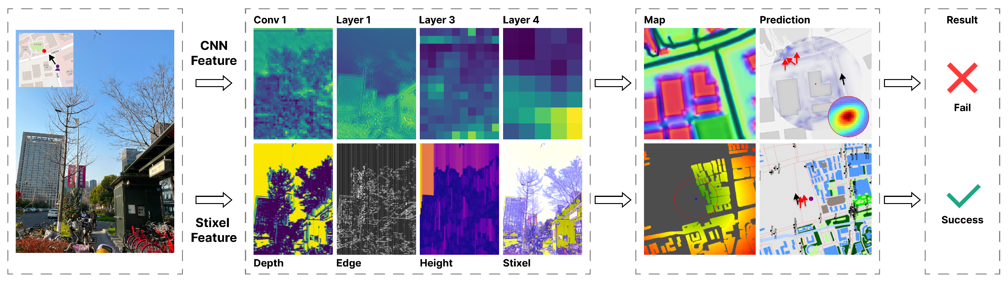
3.1. Image-CNN

The CNN $\mathrm{\Phi }$image extracts a feature map $X\in {\mathbb{R}}^{U\times V\times R}$ of size $U\times V$ from the image. Then, the image features are converted into a polar coordinate representation and subsequently mapped onto a Cartesian grid; the coordinate transformation process can be seen in Figure 3. Finally, the small CNN $\mathrm{\Phi }$BEV processes it to obtain the neural Bird’s-Eye View (BEV) T and confidence C. By predicting for each polar coordinate unit $(u,d)$, the image is regarded as being composed of multiple columns, and the pixel probability distribution is $\mathrm{\alpha }$u,d. For each column, calculate the angle between it and the center of the image, as well as the distance from the pixels on this column to the center of the image, and determine the corresponding ray in the polar coordinate system, thus obtaining $X\in {\mathbb{R}}^{U\times D\times V}$. Then, convert each pixel in the image into the corresponding point in the polar coordinate system according to its column and row positions. Next, resample the polar coordinate grid into a Cartesian grid. The size of the Cartesian grid is L × D = 32 × 32 m, and the resolution $\Delta$ = 50 cm. The CNN is ResNet101; when converting the image features into a polar coordinate representation, the sampling of D depth planes is taken into account, which involves depth-related calculations. Therefore, depth features will be generated.

3.2. Map-CNN

Here, we focus on the OSM encoding part. The Map-CNN module encodes OSM into a neural map F containing semantic and geographic information useful for localization. In this stage, geographical elements such as areas, lines, and points in OpenStreetMap are rasterized into three-channel images at a fixed ground sampling distance of 50 cm/pixel. Subsequently, each semantic class is associated with an N-dimensional embedding vector obtained through learning. On this basis, a feature map is obtained with dimensions W × H × 3N.

Finally, a convolutional neural network ${\mathrm{\Phi }}_{\mathrm{map}}$, constructed based on the VGG-16 encoder, is used to encode the feature map. As a result, a neural map F with dimensions $W\times H\times N$ is obtained. Meanwhile, ${\mathrm{\Phi }}_{\mathrm{map}}$ predicts a unary location prior $\mathrm{\Omega }$ for each cell of the map, with dimensions also being $W\times H$.

3.3. Image-OSM-Stixel

We propose a hybrid voxel-pixel method that combines traditional rule-based voxel-pixel generation and modern deep learning-based feature extraction techniques. Specifically, the generation of voxel-pixels employs a traditional segmentation method based on depth variation, maintaining computational efficiency and interpretability. For feature extraction, a combination of convolutional neural networks, statistical analysis, and Fourier transform is adopted to enhance the feature representation ability.

First, the initial step is to obtain the image-Stixel representation. The image I is input, and a depth map $D(x,y)$ is generated through edge detection, thereby obtaining the distance information of each pixel. In the specific implementation, we apply the Canny operator (with thresholds 100 and 200) to detect edges. Then, we perform a dilation operation with a 5 × 5 kernel on the detection results. The relative depth value $D(x,y)$ of each pixel is calculated through the formula $D(x,y)={\displaystyle \frac{255-\mathrm{edge\_density}(x,y)}{255}}$, thus establishing a mapping between the image structure and the depth relationship. The image I is divided into vertical strips according to the width. For each vertical strip t, the depth value $d_t$ of the current column is considered, and the depth discontinuity points are detected. The rate of depth change is $\Delta d=\left|D\right(x,y)-D(x,y+1\left)\right|$. The average of the depth values and color values of the current column are taken to obtain the depth distribution and color distribution, which respectively represent the average depth and color of each pixel in the current column. According to the boundary points of depth changes, the current column is divided into several vertical regions, and each region represents a Stixel; a Stixel sequence $A_i=\{a_1,a_2,\dots ,a_k\}$ is generated, where $a_j=(x,y_{\mathrm{bottom}},y_{\mathrm{top}},w,\mathrm{depth},\mathrm{color})$.

The color classification process of a Stixel is to classify it into ground, near objects, medium-distance objects, or distant objects according to the depth value and position attributes of each Stixel.

$$\mathrm{color}=\left\{\begin{array}{cc}(0,255,0),\hfill & \mathrm{if}{y}_{\mathrm{bottom}}=\mathrm{height}-1\left(\mathrm{ground}\right)\hfill \\ (255,0,0),\hfill & \mathrm{if}\mathrm{depth}<0.3\left(\mathrm{near}\right)\hfill \\ (0,0,255),\hfill & \mathrm{if}0.3\le \mathrm{depth}<0.6\left(\mathrm{medium}\right)\hfill \\ (255,255,0),\hfill & \mathrm{if}\mathrm{depth}\ge 0.6\left(\mathrm{distant}\right)\hfill \end{array}\right.$$

The process of converting Stixel representation into tensors is as follows:

$$T_i=[x_i,y_{\mathrm{bottom},i},y_{\mathrm{top},i},{\mathrm{width}}_i,{\mathrm{depth}}_i,R_i,G_i,B_i]$$

Use CNN to extract features of A:

$$F_{\mathrm{CNN}}=\mathrm{CNN}\left(A\right)\to {\mathbb{R}}^c$$

(1)

The statistical feature extraction process is as follows:

$$\begin{array}{cc}\hfill F_{\mathrm{STAT}}& =[\mathrm{mean},\mathrm{std},\mathrm{median},\dots ,\hfill \\ \hfill & \mathrm{percentile}25,\mathrm{percentile}75]\to {\mathbb{R}}^s\hfill \end{array}$$

(2)

The image-Stixel feature can be expressed as:

$$\begin{array}{c}\hfill F_{\mathrm{stixel}}=\left[F_{\mathrm{CNN}}\mid F_{\mathrm{STAT}}\right]\end{array}$$

(3)

Secondly, the next step is to obtain the OSM-Stixel features. Due to the existence of a prior position $P(u,v)$, a grid map M, with dimensions $L\times H\times W$, can be received. The orientation angle $\phi$ is obtained; it is calculated from the prior position $P(u,v)$, and the grid map M, and the positions of building pixels are extracted from the grid map to generate a set of building coordinates B. Through polar coordinate conversion and calculation, $\mathrm{\Theta }=[{\theta }_1,{\theta }_2,\dots ,{\theta }_n]$ and $R=[r_1,r_2,\dots ,r_n]$ are obtained. To comprehensively capture the spatial distribution characteristics of buildings, we divide the 360° space into 36 uniform intervals, each with a span of 10°. For each angular interval, $k\in [0,35]$. The weighted angular distribution feature is defined as

$$O_w\left[k\right]=\sum _{{\theta }_i\in \left[k\Delta \theta ,(k+1)\Delta \theta \right)}{r}_i$$

(4)

The unweighted angular distribution feature is defined as:

$$O_u\left[k\right]=\mathrm{count}\left({\theta }_i\right),{\theta }_i\in \left[k\Delta \theta ,(k+1)\Delta \theta \right).$$

(5)

The normalized weighted distribution is given by:

$$O_n\left[k\right]={\displaystyle \frac{O_w\left[k\right]}{{\displaystyle \sum _{j=0}^{35}}{O}_w\left[j\right]}}.$$

(6)

Within its spatial distribution range, for each angular interval, the maximum distance distribution is calculated as:

$$R_{\max }\left[k\right]=max\left\{r_i\mid {\theta }_i\in [k·\Delta \theta ,(k+1)·\Delta \theta )\right\}.$$

(7)

According to the current orientation $\phi$, the distance feature $d_{\phi }$ in the directional feature and ${\theta }^{*}$ obtained through weighted calculation are derived.

For the k-th angular interval $[k·\Delta \theta ,(k+1)·\Delta \theta )$:

$$F_{\mathrm{osm}}\left[k\right]=\left\{\begin{array}{cc}{\displaystyle \sum _{{\theta }_i\in [k·\Delta \theta ,(k+1)·\Delta \theta )}}{r}_i\hfill & \left(\mathrm{i}\right)\hfill \\ \mathrm{count}\left({\theta }_i\right),{\theta }_i\in [k·\Delta \theta ,(k+1)·\Delta \theta )\hfill & \left(\mathrm{ii}\right)\hfill \\ {\displaystyle \frac{{\displaystyle \sum _{{\theta }_i\in [k·\Delta \theta ,(k+1)·\Delta \theta )}}{r}_i}{{\displaystyle \sum _{j\in [0,35]}}{\displaystyle \sum _{{\theta }_i\in [j·\Delta \theta ,(j+1)·\Delta \theta )}}{r}_i}}\hfill & \left(\mathrm{iii}\right)\hfill \\ max\{r_i\mid {\theta }_i\in [k·\Delta \theta ,(k+1)·\Delta \theta )\}\hfill & \left(\mathrm{iv}\right)\hfill \end{array}\right.$$

where:

(i)

Distance-weighted sum of building pixels

(ii)

Pixel count in angular interval

(iii)

Normalized orientation distribution

(iv)

Maximum distance in angular interval

To ensure that the Stixel feature map and the OSM feature map are consistent in dimensions, we use the $dim\left(F_{\mathrm{stixel}}\right)=dim\left(F_{\mathrm{osm}}\right)$. A linear projection layer is employed to map features of different dimensions to a common feature space. After the two types of features are projected to a common dimension, batch normalization is applied to ensure that the features of different modalities are comparable in terms of the numerical range.

After alignment, one of the following methods is adopted for feature fusion:

Feature concatenation: $F_{fused}=[F_{stixel}\left|\right|F_{osm}]$,

Weighted fusion: $F_{fused}=\alpha ·F_{stixel}+(1-\alpha )·F_{osm}$,

Attention mechanism: $F_{fused}=Attention(F_{stixel},F_{osm})$.

3.4. Match

The distance features have significant disadvantages in the matching process, such as strong dependence on the viewing angle, sensitivity to scale, reduced accuracy at long distances, and vulnerability to environmental interference. These lead to large feature differences of the same object under different viewing angles, unstable features of near and far objects, and low quality of feature extraction. In contrast, angle feature matching successfully overcomes these defects with its good viewing angle invariance and scale adaptability. It not only enables the same object to maintain stable feature expressions under different viewing angles and distances but also performs excellently in handling distant objects and maintaining boundary details.

Suppose the probability distribution of the camera pose is denoted as $\xi$. For instance, in a complex environment, the camera may have several different reasonable positions and orientations. Each position and orientation corresponds to a possible pose, and these different possible poses form multiple peaks with relatively high probabilities. This multi-modal probability distribution enables us to easily fuse the camera pose estimation with other additional sensors, such as GPS. Calculating this probability distribution is relatively straightforward. This is because the pose space of the camera has been reduced to three dimensions. Moreover, this probability distribution is discretized to each map location, which means that we discretize the continuous space, making the calculation simpler. Sampling the rotation K times at a fixed interval avoids complex continuous calculations and improves the calculation efficiency. Therefore,

$$P\left(\xi \right|\mathrm{I},\mathrm{map},{\xi }_{\mathrm{prior}})=P\left(\xi \right).$$

(8)

The neural map F and the BEV T are thoroughly matched to obtain the score M. Each element is calculated by correlating F with the correspondingly transformed T after pose transformation. $\xi \left(p\right)$ is equivalent to a coordinate transformation that can convert the point p from the BEV coordinate system to the coordinate system corresponding to the coordinate frame of the map. The confidence level C can play a screening role. In the BEV space, there may be some parts that are unreliable and can cause interference. Through the confidence level, the correlation between these parts and other parts can be reduced. T is rotated for K times and a single convolution is performed in the Fourier domain, which can achieve efficient parallel computing.

$$M\left[\xi \right]={\displaystyle \frac{1}{UZ}}\sum _{p\in (U\times Z)}F{\left[\xi \left(p\right)\right]}^{\top }(T\odot C)\left[p\right].$$

(9)

$H_{\mathrm{stixel}}$ counts the directions of the rod-like features of the entire image, with each Stixel representing the vertical edge of a building. The number of Stixels in the image is M, the orientation angle of each Stixel is ${\beta }_{\mathrm{i}},i=1,2,3,\dots ,M$, and we divide the orientation range $[0^{\circ },{360}^{\circ }]$ into K intervals (for example, when each bin is ${10}^{\circ }$, then $K=36$). Based on the Stixel centroid $(x_c,y_c)$ and image center $(x_{\mathrm{center}},y_{\mathrm{center}})$:

$${\beta }_i=arctan2(y_c-y_{\mathrm{center}},x_c-x_{\mathrm{center}}).$$

(10)

Therefore, the Stixel feature direction of the entire image is

$$H_{\mathrm{stixel}}\left[j\right]={\displaystyle \frac{1}{M}}\sum _{i=1}^M\delta \left(j,⌊{\displaystyle \frac{{\beta }_i}{\Delta \beta }}⌋\right),j=1,2,\dots ,K.$$

(11)

The symbol $\delta$ here represents the Kronecker delta. It is equal to 1 when the two parameters match and is 0 otherwise. It is used to count the number of times an angle falls into a specific interval.

$H_{\mathrm{osm}}$ counts the directions of the building edges in the $OSM$ map and extracts the main orientations of the building outlines. The building boundaries in OSM are represented as boundary line segments of polygons. Each boundary line segment is uniquely determined by its two endpoints: $(x_1,y_1)$ and $(x_2,y_2)$. The orientation angle $\theta$ (i.e., edge direction) of each boundary line segment can be computed using:

$$\theta =arctan2(y_2-y_1,x_2-x_1).$$

(12)

$$H_{\mathrm{osm}}\left[j\right]=\sum _{i=1}^N\delta \left(j,\mathrm{bin}\left({\theta }_i\right)\right),j\in \{1,2,\dots ,K\}.$$

(13)

$H_{\mathrm{osm}}(i+\theta )$, where $\theta$ represents the rotation angle, performs a cyclic shift on the OSM angles; $w_i$ represents the weight factor applied to each bin during the angular histogram matching process.

$$S_{\mathrm{angle}}\left(\theta \right)=\sum _i{w}_{i}min(H_{\mathrm{stixel}}\left(i\right),H_{\mathrm{osm}}(i+\theta )).$$

(14)

$$S_{\mathrm{total}}(x,y,\theta )=(1-\alpha )M(x,y,\theta )+\alpha S_{\mathrm{angle}}\left(\theta \right).$$

(15)

Lastly, we fuse the two sets of features after matching.

The angle matching method based on Stixel features achieves the enhancement of features from local to global by introducing angle distribution. It naturally combines the directional information of the Stixel itself with angle matching, effectively weakening the influence of local errors and enhancing the adaptability to occlusion and sparse scenes. Meanwhile, this method can realize the efficient cross-modal alignment between the Stixel features of images and OSM maps. It quickly solves the rotation problem through angle distribution, reducing the computational complexity. It is particularly suitable for distinguishing scenes with significant directional differences. Moreover, the lightweight scheme using sparse features in combination with angle distribution significantly reduces the computational and storage costs.

Processing Mechanism for Non-Map Objects in the Scene: This paper implements a multi-level anomaly detection and filtering architecture to handle interfering objects that appear in the scene but are not present in the OSM map. This mainly includes feature confidence weighting based on semantic reliability, an adaptive outlier detector utilizing matching probabilities, graph-model filtering based on k-nearest neighbor spatial consistency, and a multi-hypothesis matching and verification strategy inspired by the RANSAC concept. These mechanisms work in concert to ensure that the system can achieve robust feature matching in complex scenarios containing a large number of dynamic objects (such as vehicles and pedestrians) and unmodeled structures.

3.5. Loss

Throughout the training process, in order to accurately estimate the pose, we utilize the Negative Log Likelihood (NLL) loss. After training and calculation, the predicted pose is p and its corresponding ground truth pose is $p^{*}$.

The formula for the localization loss is as follows:

$$L_{\mathrm{loc}}=-logP\left(p^{*}|p\right)$$

(16)

To address the inherent uncertainties in pose estimation, Gaussian smoothing is employed:

$$L_{\mathrm{loc}}=-log\left[N(x^{*}\mid x,{\sigma }_{xy})·N(y^{*}\mid y,{\sigma }_{xy})·N({\theta }^{*}\mid \theta ,{\sigma }_r)\right].$$

(17)

where ${\sigma }_{xy}$ and ${\sigma }_r$ are hyperparameters representing the standard deviations of the position components $(x,y)$ and the rotation component r in the positioning uncertainty model, respectively.

After feature matching, the obtained similarity loss is as follows:

$$L_{\mathrm{sim}}=-{\displaystyle \frac{1}{D}}\sum _i{\displaystyle \frac{{\mathbf{f}}_{{\mathrm{stixel}}_i}·{\mathbf{f}}_{{\mathrm{osm}}_i}}{\parallel {\mathbf{f}}_{{\mathrm{stixel}}_i}\parallel \parallel {\mathbf{f}}_{{\mathrm{osm}}_i}\parallel }}.$$

(18)

Therefore, in order to obtain a more accurate pose, the loss is updated as follows:

$$L_{\mathrm{total}}=L_{\mathrm{loc}}+\lambda ·L_{\mathrm{sim}}.$$

(19)

Systematic dataset experiments show that $\lambda =0.2$ yields the steadiest training curve, fastest convergence, oscillation-free training, and optimal positional-angular accuracy balance.

Algorithm Fusing Horizon Information for Visual Localization

Input: image, map, camera parameters, bev_valid Initialization: Initialize image encoder, map encoder Initialize scale classifier Initialize coordinate transformation and projection modules Initialize OSM feature extractor Update: Image feature extraction: f_image = image_encoder(image) Stixel feature extraction: (a) depth_map = estimate_depth(image) (b) stixels = generate_stixels(image, depth_map) (c) stixel_representation = stixels_to_feature_input(stixels) (d) stixel_features = stixel_extractor(stixel_tensor) Feature projection: (a) f_polar = projection_polar(f_image, scales, camera) (b) f_bev = projection_bev(f_polar) OSM feature extraction and similarity calculation: (a) angles, distances = visualize_map_with_pose_and_tile(map) (b) osm_features = extract_polar_features(angles, distances) Similarity-weighted score calculation: (a) stixel_angle_features = Compress Stixel Angular Features using Fourier Transform (b) osm_angle_features = Normalize OSM Angular Features (c) best_angle, best_similarity = find_best_rotation(stixel_normalized, osm_normalized) Score calculation: (a) scores = exhaustive_vote(f_bev, f_map, valid_bev, confidence, similarity) Loss calculation: (a) nll = nll_loss_xyr(log_probs, xy_gt, yaw_gt) (b) similarity_loss = -mean(similarity) (c) total_loss = nll + $\lambda ·$ similarity_loss

4. Experiments and Results

Experiment device

In the experimental setup, the relevant hardware and software information is presented as follows:

• Hardware: NVIDIA GeForce RTX 3090
• Code Language: python-3.9.21
• Framework: torch-2.5.1

Dataset Selection

The Mapillary Geo-Localization (MGL) dataset [23] and KITTI dataset [24] are used in this experiment, and they have the following characteristics:

• Data Source and Scale: MGL is collected from the Mapillary street view platform; it widely covers 12 major cities in Europe and America, with a total of 760,000 street view images. KITT is sourced from Karlsruhe, Germany, and its surrounding areas and was first released in 2012. It contains over 6 h of traffic scene recordings, covers a driving distance of about 39.2 km, and has over 200,000 3D-labeled objects and more than 30,000 pairs of stereo images.
• Capture Devices and Scenes: The capture devices of the MGL dataset are rich and diverse, including hand-held cameras, vehicle-mounted cameras, and bicycle-mounted cameras, thus capturing a variety of scenes, such as city streets, various buildings, and transportation facilities. Moreover, the perspectives of the images also show diversity in height and angle. The KITTI is collected using a modified Volkswagen Passat station wagon equipped with 2 PointGrey Flea2 color cameras (1392 × 512 pixels) and 2 PointGrey Flea2 grayscale cameras (1392 × 512 pixels), 1 Velodyne HDL-64E LiDAR, and 1 OXTS RT3003 high-precision GPS/IMU system. The scenes include urban roads, residential areas, highways, and rural roads and cover different weather and lighting conditions.
• Currently, studies focus on the localization technology between ground images and satellite images from different perspectives. Therefore, in addition to using OpenStreetMap (OSM), we have also employed satellite maps.
• Annotation Information and Acquisition Method: It has 6-Degree-of-Freedom pose information (6-DoF), including 3 translation parameters (x, y, z) and 3 rotation parameters (roll, pitch, yaw). This pose information is obtained through the combination of Structure from Motion (SfM) technology and GPS data fusion.

Evaluation Metrics

• Position Recall: The evaluation thresholds are set as 1 m, 3 m, and 5 m. The proportion of samples whose predicted position is within the corresponding threshold distance from the ground truth position to the total samples is calculated to evaluate the spatial accuracy of the model’s positioning.
• Orientation Recall: 1 degree, 3 degrees, and 5 degrees are used as the evaluation thresholds. The proportion of samples whose angle difference between the predicted orientation and the ground truth orientation is within the threshold is calculated to measure the accuracy of the model’s orientation estimation.
• Error Calculation: The position error is measured by the Euclidean distance between the predicted position and the ground truth position, and the orientation error is represented by the angle difference between the predicted orientation and the ground truth orientation.

Baseline Model Setup

OrienterNet is selected as the baseline model and adjusted and adapted according to the research method to ensure effective comparative analysis in the experiment.

The experiment took one and a half months to complete and used different autonomous driving scenario datasets and various positioning methods; the results are as shown in

Table 1. Comparison of lateral accuracy at different distances.

Map	Approach	Training Dataset	Lateral@Xm			Runtime
			1 m	3 m	5 m	(ms)
OpenStreetMap	retrieval [8,25]	MGL	37.47	66.24	72.89	145
	refinement [26]	MGL	50.83	78.10	82.22	210
	OrienterNet [3]	MGL	53.51	88.85	94.47	125
	BEV + Stixel	MGL	56.00	88.20	95.10	85
	BEV + Angle	MGL	54.80	89.50	94.70	80
	Ours	MGL	57.25	87.65	95.62	105
Satellite	DSM [27]	KITTI	10.77	31.37	48.24	180
	VIGOR [28]	KITTI	17.38	48.20	70.79	155
	refinement [26]	KITTI	27.82	59.79	72.89	210
	OrienterNet [3]	KITTI	51.26	84.77	91.81	125
	BEV + Stixel	KITTI	53.50	84.10	92.00	87
	BEV + Angle	KITTI	53.00	85.00	92.50	82
	Ours	KITTI	54.84	83.56	92.35	107

,

Table 2. Comparison of longitudinal recall at different distances.

Map	Approach	Training Dataset	Longitudinal R@Xm			Runtime
			1 m	3 m	5 m	(ms)
OpenStreetMap	retrieval [8,25]	MGL	5.94	16.88	26.97	145
	refinement [26]	MGL	17.75	40.32	52.40	210
	OrienterNet [3]	MGL	26.25	59.84	70.76	125
	BEV + Stixel	MGL	27.50	62.00	71.00	85
	BEV + Angle	MGL	26.80	61.50	70.90	80
	Ours	MGL	28.07	63.73	71.51	105
Satellite	DSM [27]	KITTI	3.87	11.73	19.50	180
	VIGOR [28]	KITTI	4.07	12.52	20.14	155
	refinement [26]	KITTI	5.75	16.36	26.48	210
	OrienterNet [3]	KITTI	22.39	46.79	57.81	125
	BEV + Stixel	KITTI	23.00	48.50	60.50	87
	BEV + Angle	KITTI	22.80	47.50	58.50	82
	Ours	KITTI	23.4	49.83	61.27	107

and

Table 3. Comparison of orientation recall at different angles.

Map	Approach	Training Dataset	Orientation R@X°			Runtime
			1°	3°	5°	(ms)
OpenStreetMap	retrieval [8,25]	MGL	2.97	12.32	23.27	145
	refinement [26]	MGL	31.03	66.76	76.07	210
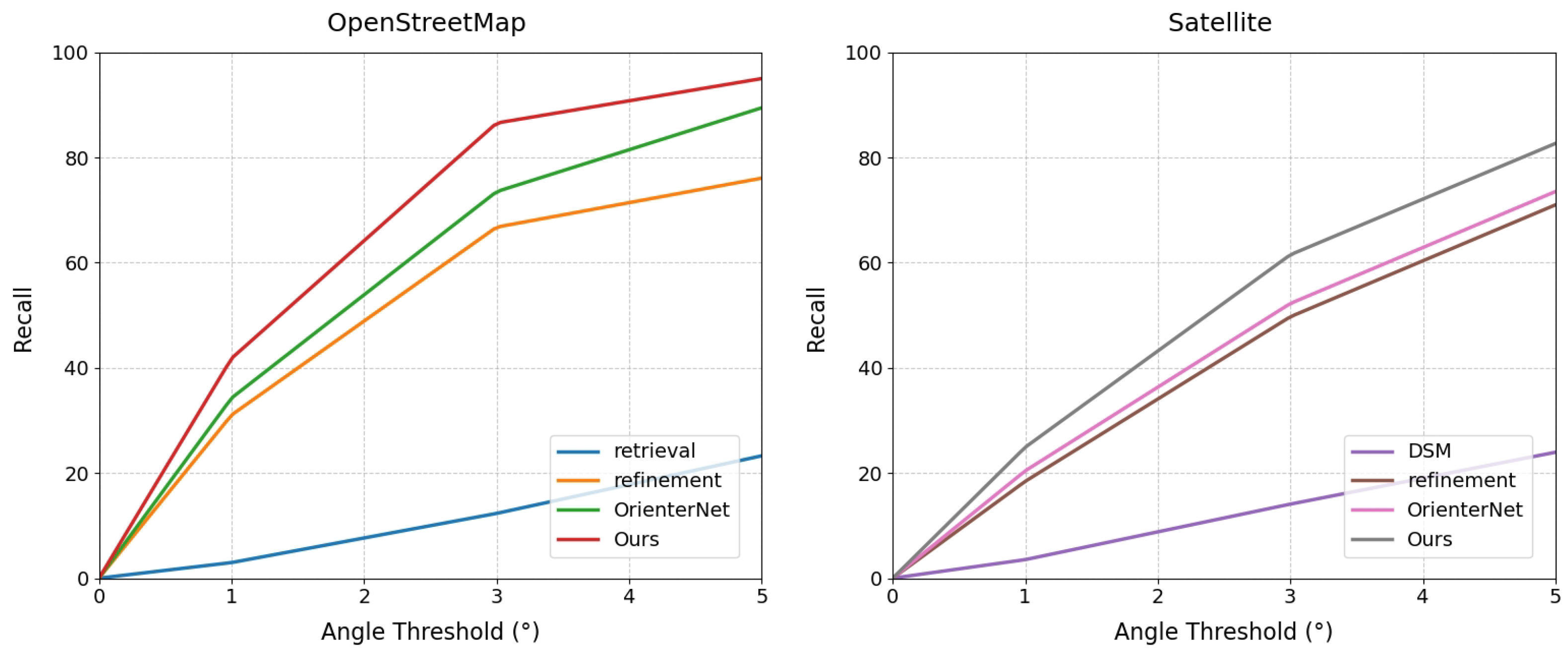
	OrienterNet [3]	MGL	34.26	73.51	89.45	125
	BEV + Angle	MGL	40.80	85.20	94.70	80
	BEV + Stixel	MGL	36.50	75.00	89.80	85
	Ours	MGL	41.80	86.55	95.01	105
Satellite	DSM [27]	KITTI	3.53	14.09	23.95	180
	VIGOR [28]	KITTI	-	-	-	155
	refinement [26]	KITTI	18.42	49.72	71.00	210
	OrienterNet [3]	KITTI	20.41	52.24	73.53	125
	BEV + Angle	KITTI	24.00	60.00	81.50	82
	BEV + Stixel	KITTI	22.00	55.00	78.00	87
	Ours	KITTI	24.90	61.51	82.68	107

. When trained on the KITTI dataset, in terms of lateral and longitudinal positional errors, the localization recall rate of our proposed FHVL method is higher than that of other methods. When trained on the MGL dataset, in terms of positional errors, it is also slightly higher than other methods. Additionally, as depicted in Figure 4, in terms of the recall rate of orientation positions on both datasets, the FHVL method outperforms other methods more significantly and exhibits more robust performance. As shown in Figure 5, the model can accurately capture features such as building contours in typical urban scenes, with minimal error between the predicted position and the ground truth, further validating the improvement of positioning accuracy through multi-modal feature fusion. These experimental indicators are all kept consistent with those of the baseline experiment.

5. Algorithm Complexity Analysis

Time Complexity

• OrienterNet: The dominant computational step is exhaustive voting with complexity $O\left(R{M}^2{N}^2\right)$. Other steps include feature extraction $O\left(CHW\right)$, BEV projection $O\left(CDH\right)$, etc.
• Our Method: Additional computations introduced on top of OrienterNet:

  –

  Stixel generation and feature extraction: $O(W{D}_s+S·C_s)$

  –

  OSM feature extraction: $O\left(B\right)$

  –

  Similarity computation: $O\left(C_f\right)$

  –

  Additional voting step: $O\left(R{M}^2{N}^2\right)$

  Overall Complexity: $O(2R{M}^2{N}^2+CHW+CDH+C{M}^2+\mathrm{other}\mathrm{minor}\mathrm{terms})$
• Theoretical Complexity: The theoretical complexity is approximately twice that of the original method, dominated by the two voting operations.
• Actual Runtime: The average measured increase is 46%, attributed to:

  –

  Reuse of intermediate results through hardware acceleration

  –

  Parallel execution of Stixel and OSM feature extraction

  –

  Reduced computational load via compressed feature representations

Space Complexity

• OrienterNet: Major memory overheads include BEV features $O\left(C{N}^2\right)$ and voting templates $O\left(RC{N}^2\right)$.
• Our Method: Additional memory requirements:

  –

  Depth map: $O\left(HW\right)$

  –

  Stixel and OSM features: $O(SW+C_o)$

  –

  Second score tensor: $O\left(R{M}^2\right)$

  Overall Complexity: $O(RC{N}^2+C{M}^2+2R{M}^2+\mathrm{other}\mathrm{minor}\mathrm{terms})$
• Summary: The primary increase comes from storing the second score tensor, which is relatively small compared to the original method’s total memory footprint.

Model Parameters

• Additional Stixel feature extractor: ∼68 K parameters
• Extra feature projection layers: ∼4 K parameters
• Total increase: $0.5\%$ relative to OrienterNet’s $14.5\mathrm{M}$ parameters

6. Conclusions

Firstly, the model we proposed incorporates a multi-modal feature fusion mechanism, effectively integrating BEV features, Stixel structural features, and OpenStreetMap (OSM) features, providing a more comprehensive scene understanding ability. Secondly, by introducing a geometric-constraint-based similarity calculation mechanism, the model can more accurately evaluate the consistency between different features, thereby improving the positioning accuracy. These improvements enable the model to better handle complex real-world scenarios, reduce the dependence on a single feature, and enhance the model’s adaptability to environmental changes. Experimental results show that the model we proposed has achieved significant improvements in positioning accuracy, orientation estimation, and scene understanding, demonstrating stronger practical value and generalization ability. Future optimizations focus on three aspects: integrating multi-sensor data (e.g., LiDAR, radar) into the heterogeneous framework via customized extractors to enhance robustness in harsh environments; introducing temporal similarity metrics and feature accumulation to improve continuous localization consistency/accuracy for autonomous driving/robot navigation; developing dynamic feature importance evaluation to adaptively adjust feature dependency based on environmental changes, strengthening generalization/stability across scenarios.

References

- Zhang, J.; Singh, S. LOAM: Lidar Odometry and Mapping. In Proceedings of the IEEE/RSJ International Conference on Intelligent Robots and Systems (IROS), Chicago, IL, USA, 14–18 September 2014; pp. 1271–1278. [Google Scholar]
- Zhao, B.; Yang, L.; Mao, M.; Bao, H.; Cui, Z. Pnerfloc: Visual localization with point-based neural radiance fields. Proc. AAAI Conf. Artif. Intell. 2024, 38, 7450–7459. [Google Scholar] [CrossRef]
- Sarlin, P.; DeTone, D.; Yang, T.; Avetisyan, A.; Straub, J.; Malisiewicz, T.; Bulo, S.; Newcombe, R.; Kontschieder, P.; Balntas, V. OrienterNet: Visual localization in 2D public maps with neural matching. In Proceedings of the IEEE/CVF Conference on Computer Vision and Pattern Recognition, Vancouver, BC, Canada, 17–24 June 2023; pp. 21632–21642. [Google Scholar]
- Li, Q.; Wang, Y.; Wang, Y.; Zhao, H. Hdmapnet: An online hd map construction and evaluation framework. In Proceedings of the 2022 International Conference on Robotics and Automation (ICRA), Philadelphia, PA, USA, 23–27 May 2022; IEEE: Piscataway, NJ, USA, 2022; pp. 4628–4634. [Google Scholar]
- Muñoz-Bañón, M.A.; Velasco-Sánchez, E.; Candelas, F.A.; Torres, F. Openstreetmap-based autonomous navigation with lidar naive-valley-path obstacle avoidance. IEEE Trans. Intell. Transp. Syst. 2022, 23, 22284–22296. [Google Scholar] [CrossRef]
- Barros, T.; Garrote, L.; Pereira, R.; Premebida, C.; Nunes, U.J. Improving localization by learning pole-like landmarks using a semi-supervised approach. In Proceedings of the Robot 2019 The Fourth Iberian Robotics Conference, Porto, Portugal, 20–22 November 2020; Silva, M.F., Lima, J.L., Reis, L.P., Sanfeliu, A., Tardioli, D., Eds.; Springer International Publishing: Cham, Switzerland, 2020; pp. 255–266. [Google Scholar]
- Levi, D.; Garnett, N.; Fetaya, E.; Herzlyia, I. Stixelnet: A deep convolutional network for obstacle detection and road segmentation. In Proceedings of the British Machine Vision Conference 2015, Swansea, UK, 7–10 September 2015; Volume 1, p. 4. [Google Scholar]
- Samano, N.; Zhou, M.; Calway, A. You are here: Geolocation by embedding maps and images. In Proceedings of the Computer Vision—ECCV 2020: 16th European Conference, Glasgow, UK, 23–28 August 2020; Springer: Cham, Switzerland, 2020; pp. 502–518. [Google Scholar]
- O’Keefe, J.; Nadel, L. The Hippocampus as a Cognitive Map; Clarendon Press: Oxford, UK, 1978. [Google Scholar]
- Park, C.; Seo, E.; Lim, J. Heightlane: Bev heightmap guided 3d lane detection. arXiv 2024, arXiv:2408.08270. [Google Scholar]
- Wang, R.; Qin, J.; Li, K.; Li, Y.; Cao, D.; Xu, J. Bev-lanedet: A simple and effective 3d lane detection baseline. arXiv 2023, arXiv:2210.06006. [Google Scholar]
- He, Y.; Liang, S.; Rui, X.; Cai, C.; Wan, G. Egovm: Achieving precise ego-localization using lightweight vectorized maps. In Proceedings of the 2024 IEEE/RSJ International Conference on Intelligent Robots and Systems (IROS), Abu Dhabi, United Arab Emirates, 14–18 October 2024; IEEE: Piscataway, NJ, USA, 2024; pp. 12248–12255. [Google Scholar]
- Lin, Z.; Wang, Y.; Qi, S.; Dong, N.; Yang, M.H. Bev-mae: Bird’s eye view masked autoencoders for point cloud pre-training in autonomous driving scenarios. arXiv 2024, arXiv:2212.05758. [Google Scholar] [CrossRef]
- Wu, H.; Zhang, Z.; Lin, S.; Mu, X.; Zhao, Q.; Yang, M.; Qin, T. Maplocnet: Coarse-to-fine feature registration for visual re-localization in navigation maps. In Proceedings of the 2024 IEEE/RSJ International Conference on Intelligent Robots and Systems (IROS), Abu Dhabi, United Arab Emirates, 14–18 October 2024; IEEE: Piscataway, NJ, USA, 2024; pp. 13198–13205. [Google Scholar]
- Sarlin, P.; Trulls, E.; Pollefeys, M.; Hosang, J.; Lynen, S. Snap: Self-supervised neural maps for visual positioning and semantic understanding. Adv. Neural Inf. Process. Syst. 2023, 36, 7697–7729. [Google Scholar]
- Lobben, A.K. Navigational map reading: Predicting performance and identifying relative influence of map-related abilities. Ann. Assoc. Am. Geogr. 2007, 97, 64–85. [Google Scholar] [CrossRef]
- Zhu, S.; Shah, M.; Chen, C. TransGeo: Transformer Is All You Need for Cross-view Image Geo-localization. arXiv 2022, arXiv:2204.00097. [Google Scholar]
- Sun, J.; Shen, Z.; Wang, Y.; Bao, H.; Zhou, X. LoFTR: Detector-Free Local Feature Matching with Transformers. In Proceedings of the IEEE/CVF Conference on Computer Vision and Pattern Recognition (CVPR), Nashville, TN, USA, 20–25 June 2021; pp. 1–9. [Google Scholar]
- Yin, H.; Wang, Y.; Tang, L.; Ding, X. LocNet: Global Localization in 3D Point Clouds for Mobile Robots. In Proceedings of the 2018 IEEE Intelligent Vehicles Symposium (IV), Changshu, China, 26–30 June 2018; IEEE: Piscataway, NJ, USA, 2018; pp. 1355–1360. [Google Scholar]
- Bai, X.; Hu, Z.; Zhu, X.; Huang, Q.; Chen, Y.; Fu, H.; Tai, C.-L. TransFusion: Robust LiDAR-Camera Fusion for 3D Object Detection with Transformers. In Proceedings of the IEEE/CVF Conference on Computer Vision and Pattern Recognition (CVPR), New Orleans, LA, USA, 18–24 June 2022; pp. 1–10. [Google Scholar]
- Cordts, M.; Omran, M.; Ramos, T.; Rehfeld, M.; Enzweiler, R.; Benenson, U.; Franke, S.; Roth, B.; Schiele, B. The cityscapes dataset for semantic urban scene understanding. In Proceedings of the IEEE Conference on Computer Vision and Pattern Recognition, Las Vegas, NV, USA, 27–30 June 2016; IEEE: Piscataway, NJ, USA, 2016; pp. 3213–3223. [Google Scholar]
- Omama, M.; Inani, P.; Paul, P.; Yellapragada, S.C.; Jatavallabhula, K.M.; Chinchali, S.; Krishna, M. Alt-pilot: Autonomous navigation with language augmented topometric maps. arXiv 2023, arXiv:2310.02324. [Google Scholar]
- Antequera, M.L.; Gargallo, P.; Hofinger, M.; Bulo, S.R.; Kuang, Y.; Kontschieder, P. Mapillary planet-scale depth dataset. In Proceedings of the European Conference on Computer Vision, Glasgow, UK, 23–28 August 2020; Springer: Cham, Switzerland, 2020; pp. 3–4. [Google Scholar]
- Geiger, A.; Lenz, P.; Stiller, C.; Urtasun, R. Vision meets robotics: The kitti dataset. Int. J. Robot. Res. 2013, 32, 1231–1237. [Google Scholar] [CrossRef]
- Xia, Z.; Booij, O.; Manfredi, M.; Kooij, J.F. Visual cross-view metric localization with dense uncertainty estimates. In Proceedings of the European Conference on Computer Vision, Tel Aviv, Israel, 23–27 October 2022; Springer: Cham, Switzerland, 2022; pp. 2–13. [Google Scholar]
- Shi, Y.; Li, H. Beyond cross-view image retrieval: Highly accurate vehicle localization using satellite image. In Proceedings of the IEEE/CVF Conference on Computer Vision and Pattern Recognition, New Orleans, LA, USA, 18–24 June 2022; IEEE: Piscataway, NJ, USA, 2022; pp. 2–13. [Google Scholar]
- Shi, Y.; Yu, X.; Campbell, D.; Li, H. Where am i looking at? Joint location and orientation estimation by cross-view matching. In Proceedings of the IEEE/CVF Conference on Computer Vision and Pattern Recognition, Seattle, WA, USA, 13–19 June 2020; IEEE: Piscataway, NJ, USA, 2020; pp. 2–7. [Google Scholar]
- Zhu, S.; Yang, T.; Chen, C. Vigor: Crossview image geo-localization beyond one-to-one retrieval. In Proceedings of the IEEE/CVF Conference on Computer Vision and Pattern Recognition, Nashville, TN, USA, 20–25 June 2021; IEEE: Piscataway, NJ, USA, 2021; pp. 2–7. [Google Scholar]