GT-STAFG: Graph Transformer with Spatiotemporal Attention Fusion Gate for Epileptic Seizure Detection in Imbalanced EEG Data

Abstract

Background: Electroencephalography (EEG) assists clinicians in diagnosing epileptic seizures by recording brain electrical activity. Existing models process spatiotemporal features inefficiently either through cascaded spatiotemporal architectures or static functional connectivity, limiting their ability to capture deeper spatial–temporal correlations. Objectives: To address these limitations, we propose a Graph Transformer with Spatiotemporal Attention Fusion Gate (GT-STAFG). Methods: We analyzed 18-channel EEG data sampled at 200 Hz, transformed into the frequency domain, and segmented into 30- second windows. The graph transformer exploits dynamic graph data, while STAFG leverages self-attention and gating mechanisms to capture complex interactions by augmenting graph features with both spatial and temporal information. The clinical significance of extracted features was validated using the Integrated Gradients attribution method, emphasizing the clinical relevance of the proposed model. Results: GT-STAFG achieves the highest area under the precision–recall curve (AUPRC) scores of 0.605 on the TUSZ dataset and 0.498 on the CHB-MIT dataset, surpassing baseline models and demonstrating strong cross-patient generalization on imbalanced datasets. We applied transfer learning to leverage knowledge from the TUSZ dataset when analyzing the CHB-MIT dataset, yielding an average improvement of 8.3 percentage points in AUPRC. Conclusions: Our approach has the potential to enhance patient outcomes and optimize healthcare utilization.

1. Introduction

Epilepsy is a neurological disorder affecting around 50 million people around the world [1]. Epileptic seizures involve abnormal brain electrical activity which is characterized by sudden and excessive discharges that disrupt neural communication. These discharges affect the brain neurotransmitters, causing sensory disturbances, and may lead to loss of consciousness, which can be life-threatening. EEGs help clinicians measure and record brain activity to diagnose different types of seizures based on visually inspected electrical patterns. Diagnosing epileptic events heavily relies on the clinicians’ expertise to analyze EEG recordings, which is demanding and time-consuming. Clinicians often examine EEG pages spanning 10 to 20 s each and sometimes require more pages for accurate diagnosis [2,3]. To assist with faster analysis, and alleviate the burden of the manual reviewing process, developing automatic seizure recognition algorithms is highly desirable.

The advent of deep learning has revolutionized the field of epileptic seizure recognition, showing promising results. Key architectures in EEG data analysis include Convolutional Neural Networks (CNNs), Recurrent Neural Networks (RNNs) [4], Graph Neural Networks (GNNs) [5], and transformers [6]. Although CNNs are widely used for seizure recognition [7], they struggle to capture spatial dependencies and complex interactions between different brain regions [8]. Additionally, their spatial receptive field is limited by their kernel size. RNN suffers from vanishing gradients, heavily affecting the performance on long EEG sequences. Both CNNs and RNNs do not take the spatial arrangement and proximity of EEG electrodes, which is not true for EEG data. GNNs address these limitations by modeling EEG data as graphs, with nodes representing electrodes and edges representing structural or functional connectivity [9]; however, they still encounter limitations.

Graph Convolution Networks (GCNs) have been utilized across various domains for EEG analysis [8]. GCNs generalize a convolution operation on graphs through a message-passing mechanism, where features from neighboring nodes are aggregated. Adding more layers allows aggregation of information from distant nodes, but can lead to over-smoothing, where node features become diluted. This reduction in feature diversity impacts the expressiveness of GNNs, which can potentially lead to poor generalization performance. Unlike GCNs, Graph Attention Networks (GATs) employ multi-headed attention mechanisms rather than fixed convolution operations [10]. This design enables the model to dynamically determine the importance of neighboring nodes, effectively capturing complex relationships within the graph structure. However, their attention mechanism design limits the ability to capture full-graph context, reducing effectiveness in identifying interactions between distant brain regions during seizures. Additionally, GATs are not able to process edge features, which limits their ability to capture interactions in functional connectivity

While some works extended attention to all graph nodes for global attention, this increases computational complexity and limits inductive bias which is considered important in graph structure learning [11]. Graph transformers (GTs) overcome this limitation by extending the message passing with self-attention mechanism akin to transformers. They also leverage a structural (spatial) positional encoding (SPE) that captures global graph structure, all while keeping graphs sparse. Additionally, it allows processing edge features and incorporating them into the attention mechanism. In EEG analysis, SPE can be leveraged to provide spatial information through graph connectivity [11]. However, existing GTs are limited to exploiting structural aspects in graphs, such as those in protein molecules and social networks.

Since EEG data features both spatial and temporal properties, employing models that utilize architectures that exploit both spatial and temporal features are required. In the case of GNNs, it requires architectures capable of leveraging temporal dependencies, such as RNNs. This combination results in Spatiotemporal GNNs (STGNNs), which are widely used in fields like traffic forecasting and human kinematics [12]. Although STGNNs have been applied to EEG tasks, few studies have thoroughly explored their capabilities [13,14]. Transformers are now favored over RNNs for their scalability and ability to handle long-range dependencies [15]. Consequently, transformers are increasingly used in EEG research [16,17]. Spatial features are often extracted via CNNs or channel attention modules, while temporal patterns are captured using transformers. However, full self-attention in transformers demands high computational resources in addition to a well-crafted positional encoding to implicitly represent EEG electrodes connectivity.

A notable limitation of the previously mentioned models, which combine multiple architectures, is the sequential processing of spatial–temporal properties. The design of these models typically depends on cascaded processing, where the spatial processing is performed first, followed by the extraction of temporal information from the preprocessed spatial features. This sequential design prevents spatial and temporal features from interacting effectively during the learning process, as the spatial features are compressed into a fixed representation before the temporal processing. Such an information bottleneck results in the loss of crucial spatial information that could influence temporal feature learning, especially in tasks sensitive to subtle brain dynamics, like seizure detection. Consequently, cascaded models inherently struggle to capture complex interactions between spatial and temporal aspects of EEG data.

These issues combined make cascaded models struggle to capture complex spatial and temporal interdependencies, such as how subtle spatial events evolve over time. In [18], a Diffusion Convolution Gated Recurrent Unit (DCGRU) was employed to capture spatial and temporal information through a tightly coupled approach. In this model, the standard matrix multiplication in GRUs is replaced with diffusion convolution operations combined with a temporal gating mechanism, which enables the GRU to process graph structures. Although this integration is more sophisticated than fully cascaded models with completely separate spatial–temporal processing, the model still fundamentally adopts a sequential spatial-then-temporal approach. Spatial relationships are first captured through diffusion convolutions, then the GRU gates for temporal processing are updated using these preprocessed spatial features. Additionally, the assumption that spatial connectivity is static over time contradicts with the inherently dynamic nature of EEG data. A promising advantage of graph transformers is their potential to integrate temporal positional encoding (TPE) with structural (spatial) positional encoding, thereby eliminating the sequential spatial–temporal processing; however, effectively combining these positional encodings remains a challenge.

To address the challenges presented by cascaded models and fully exploit the dynamic complexity of EEG signals, it is essential to enable adaptive and simultaneous interaction between spatial and temporal features. Thus, motivated by the potential of graph transformers, and inspired by the attention mechanisms in kinematics [19], we contribute the following:

• To the best of our knowledge, we are the first to propose a graph transformer (GT) integrating both spatial and temporal positional encodings for cross-patient seizure detection. The original graph transformer is extended to additionally handle temporal graph sequences with dynamic and evolving functional brain connectivity for EEG seizure detection, omitting the need for a cascaded model design.
• We propose a Spatiotemporal Attention Fusion Gate (STAFG) technique that incorporates self-attention and a fusion gate mechanism to dynamically combine spatial and temporal positional encodings. This technique constructs node embeddings augmented with spatiotemporal information to enhance the learning potential of the original graph transformer.
• We perform cross-patient evaluation in addition to transfer learning experiments to demonstrate the robustness of the proposed model in realistic clinical settings.
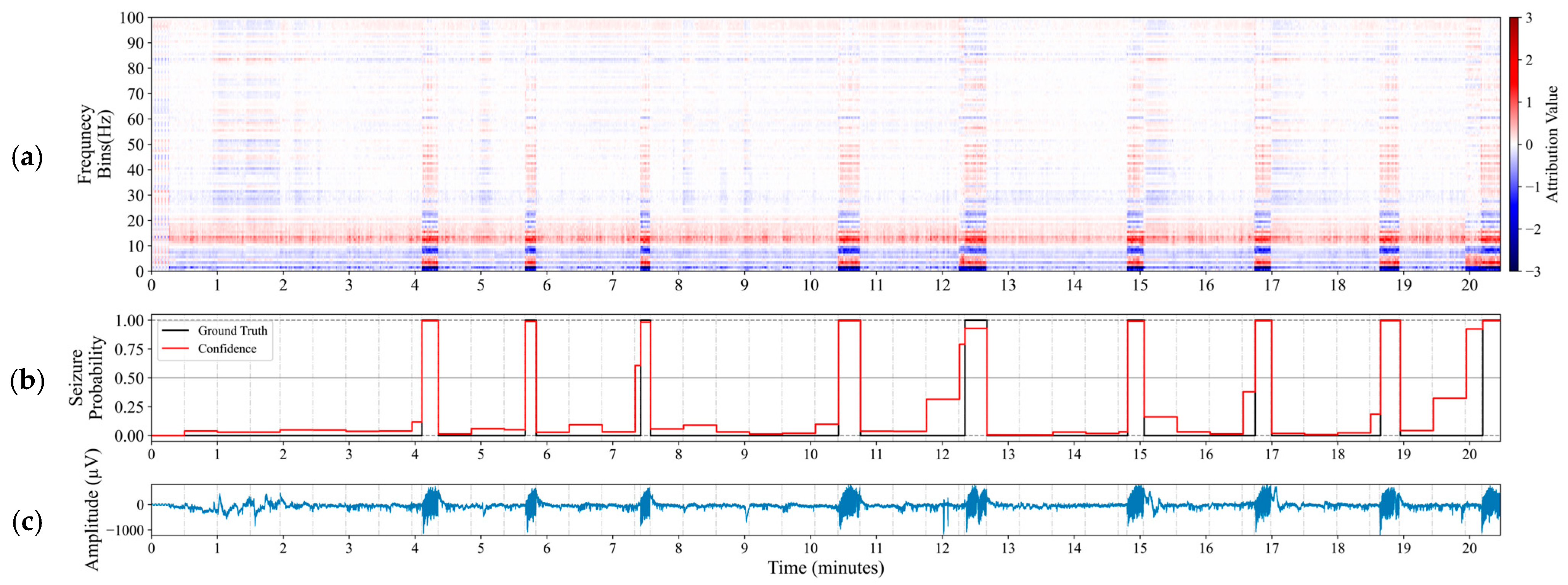
• We utilize Integrated Gradients attribution method to reveal influential frequency bands for identifying seizures and assess the relevance of the proposed model with established clinical biomarkers.

The remainder of the paper is structured as follows: Section 2 reviews related work. Section 3 details the proposed model design and methodology. Section 4 describes the datasets, preprocessing steps, and experimental settings. And Section 5 presents the experimental results and discusses this work. Finally, Section 6 concludes this work and outlines future research directions.

2. Related Works

Recent works in seizure detection have employed deep learning to analyze complex EEG patterns by combining spatial and temporal information. This section reviews key approaches, ranging from CNNs and GNNs to transformers, advancing the contribution of deep learning approaches in leveraging EEG data for epileptic seizure analysis.

2.1. Deep Learning for Seizure Detection

Epileptic seizures exhibit diverse patterns, making precise detection critical for prompt intervention. Recently, much research has been dedicated to developing advanced deep learning models to improve the accuracy and dependability of seizure detection models.

Li et al. [20] proposed CE-stSENet, a spectral–temporal model which leverages EEG’s features using squeeze-and-excitation blocks to improve seizure detection and classification. Peng et al. [21] enhanced EEGNet with sinusoidal temporal information, similar to transformers [15], to expand its receptive field. Thuwajit et al. [22] presented EEGWaveNet, a multi-scale convolution model which is designed to capture complex temporal patterns. While CNNs can effectively exploit short-term dependencies, their performance declines with longer sequences. This limitation arises since CNNs typically rely on fixed-size kernels, which constrain their temporal receptive field. As a result, CNNs struggle to effectively model relationships between distant time points, which are crucial in seizure dynamics, consequently affecting their ability to capture long-term temporal patterns.

2.2. Spatiotemporal Graph Neural Networks

STGNNs excel in capturing spatial structures through using GNNs and temporal dependencies using RNNs. This combination provides advanced architecture for analyzing complex EEG patterns. Tang et al. [18] proposed a model for both seizure detection and classification. The model captures spatiotemporal dependencies by modeling EEG data as a graph sequence. EEG recordings are segmented into 1 s intervals and grouped into a maximum sequence length of either 12 s or 60 s clips. Electrode geometry and functional connectivity are modeled using cross-correlation. As previously mentioned, this model, named Diffusion Convolution Recurrent Neural Network (DCRNN), utilizes DCGRU blocks which assume static spatial structure across EEG clips. Although this captures changes in channel (node) features across time, functional connectivity remains static across a clip, which limits the model’s ability to capture evolving and dynamic functional connectivity patterns over time.

Wang et al. [23] proposed a spatiotemporal graph attention network (STGAT) model for seizure prediction, combining graph attention network (GAT) for spatial exploration and GRUs for temporal dynamics. EEG data is represented as graphs, where functional connectivity is modeled using the Phase Locking Value (PLV). While the model accounts for changes in functional connectivity (edges) across time, the adjacency matrix is binarized. This binarization limits the model’s ability to learn from the intensity of the edge features, which hinders the potential to capture subtle variations in functional connectivity.

Feng et al. [24] proposed a spatial–temporal graph convolutional Long Short-Term Memory (ST-GCLSTM) model for EEG-based emotion recognition. This hybrid model combines a spatial graph convolutional network (SGCN) with an attention-enhanced bidirectional LSTM (Bi-LSTM) to capture EEG dynamics. The SGCN layers extract spatial features while the attention-based Bi-LSTM learns temporal patterns. The functional connectivity for the graph EEG data is computed based on Pearson’s correlation coefficient (PCC) of different frequency sub-bands, resulting in a static functional connectivity graph for each sequence. Since each processed EEG graph connectivity is static, temporal evolution within a given sequence is not captured.

He et al. [13] proposed a graph attention network with a bidirectional LSTM (GAT + Bi-LSTM) model for seizure detection. In this model, the GAT captures spatial relationships between channels, while the Bi-LSTM models temporal dynamics. It relies on fully connected graphs derived from the correlation matrix, and because the spatial module uses attention, the computational cost can rise significantly.

Shan et al. [14] proposed a spatiotemporal graph convolutional network (ST-GCN) model for Alzheimer classification. They experiment with EEG graphs constructed from different functional connectivity measures, such as PCC, PLV, phase lag index (PLI), magnitude squared coherence (MSC), imaginary part of coherence (IPC), and wavelet coherence (WC). GCN layers leverage the statically constructed adjacency matrix for spatial exploitation, while the temporal dynamics are learned via 1D convolutions. As with the GAT model, using a fully connected adjacency matrix can substantially increase computational cost.

2.3. Transformers and Self-Attention

Transformers excel in capturing long-range dependencies, making them highly effective for identifying complex temporal patterns in EEG data. However, they face challenges with spatial data. To address this challenge, CNNs are often employed to extract spatial features from EEG channels, combining the strengths of both architectures for a more comprehensive EEG analysis.

Li et al. [16] proposed a spatial–temporal (ST) transformer model for EEG brain decoding. This model leverages 1D convolutions and a channel attention module to extract spatial features, while a transformer encoder is then applied to capture temporal features.

Yang et al. [17] proposed a bio-signal transformer (BIOT) for various EEG tasks featuring a tokenization module and a linear transformer encoder. EEG recordings are divided into segments, embedded, and combined with spatial (channel) and relative positional (temporal) embeddings via a sum operation. This fusion method assumes equal importance of spatial and temporal information, restricting the model’s flexibility to capture seizure-specific patterns. The resulting restriction may not capture subtle interactions that are critical for accurately modeling brain dynamics during seizures. Moreover, both ST-TRANSFORMER and BIOT struggle to capture functional connectivity, since it was not inherently modeled, which is essential for learning interactions between different brain regions.

Wang et al. [25] introduced a hierarchical spatial-learning transformer (HSLT) for emotion recognition. The model captures spatial structures at multiple scales by grouping electrodes into regions on the scalp. A transformer encoder at the electrode level learns local spatial dependencies, while a second encoder at the region-to-region level captures interactions among brain regions. Although this design effectively models intra-region and inter-region spatial relationships, it does not explicitly address temporal sequences and thus, it may overlook fine-grained temporal dynamics.

Wan et al. [26] proposed EEGformer, which consists of three sequential transformer modules: regional, synchronous, and temporal. The regional module focuses on learning local spatial patterns within channel groups. The synchronous module captures global inter-channel correlations. Finally, the temporal module models temporal dependencies. Sequentially stacking three transformer modules result in a model with high computational demands.

Zhao et al. [27] proposed a convolutional transformer network (CTNet) model for motor imaginary classification. The model utilizes CNN architecture inspired by EEGNet [28] to learn local spatial filters. Those feature sequences are passed to a transformer encoder, which can model long-range temporal dependency interactions across all channels’ features globally.

Xiang et al. [29] proposed a synchronization-based graph spatial–temporal attention network (SGSTAN) model for seizure prediction. In this model, GAT is used for exploiting spatial features, while a transformer encoder is used for learning temporal patterns. Static brain graphs are computed based on PLV. Since the graphs are static, it limits the model’s ability to track fine changes in the functional connectivity.

3. Methods

A typical seizure detection workflow involves recording EEG signals via brain electrodes, preprocessing the data to reduce noise and artifacts, and splitting it into time segments to facilitate machine learning analysis, followed by any additional processing needed. The preprocessed EEG data is fed to a detection model to obtain results. A fine-tuning step may be required later to improve its performance on specific tasks or other datasets related. In our proposed model, the EEG signals are first transformed into the frequency domain. Afterwards, sequential graph structures (EEG clips) are constructed to allow for a comprehensive analysis of spatiotemporal relationships of the EEG data. Finally, the proposed deep learning model is trained and fine-tuned for optimal detection performance.

3.1. Preliminaries

An EEG clip graph $\mathcal{G}$ is defined as a variable-length sequence of graphs. A single graph within the sequence is represented as ${\mathcal{G}}_t=\left\{\mathcal{V},\mathcal{E},\mathit{A}\right\}$, where $\mathcal{V}$ denotes a set of nodes (electrodes), $\mathcal{E}$ denotes a set of edges (functional connectivity), $\mathit{A}$ is the adjacency matrix, and $t$ represents the position of a graph within the sequence. A graph edge is constructed as shown in [18], where ${\mathit{A}}_{i,j}=\left|h_i\ast h_j\right|$ if $v_j\in 𝒩\left(v_i\right)$, else 0. Here, $h_i$ and $h_j$ denote the node features for $v_i$ and $v_j$, respectively, $\ast$ represents normalized cross-correlation operation, and $𝒩\left(v_i\right)$ refers to the top-$\tau$ neighbor nodes of $v_i$. For each node, only its top-$\tau$ edges are retained, resulting in a sparser graph structure for each ${\mathcal{G}}_t$.

3.2. Proposed Spatiotemporal Attention Fusion Gate

To allow a node to perceive its relative spatial position in a graph and temporal position in a sequence, positional encodings are necessary. Dwivedi et al. proposed two structural (spatial) positional encodings (SPE): Laplacian eigenvalues as a positional encoding (LPE) [11] and random walks positional encoding (RWPE) [30]. We employ these two positional encodings as SPE. For temporal positional encoding (TPE), we employ the original sine and cosine functions introduced in [15].

Firstly, all node $h$ and edge $e_{ij}$ features, along with SPE and TPE, are each processed through their respective embedding layer $E_d$, with a hidden dimension size $d$. This results in node $h^l$ and edge $e_{ij}^l$embeddings. Both SPE and TPE are embedded to produce positional encoding (PE) embeddings ${SPE}^l$ and ${TPE}^l$, with the same embedding dimension as the node and edge embeddings. Afterwards, the node embeddings $h^l$, SPE embeddings ${SPE}^l,$ and TPE embeddings ${TPE}^l$ are fed to the proposed Spatiotemporal Attention Fusion Gate (STAFG). Secondly, to enrich the node representations with spatially aware context, a target node embedding $h_i^l$, a set of neighbor node embeddings $\left\{h_j^l\right\}$, and ${SPE}^l$ are passed to a self-attention spatial module. This module enables the model to focus on node feature similarity in relation to spatial adjacency. Similarly, the target node and set of neighboring nodes, along with ${TPE}^l$, are passed to a self-attention temporal module, which enables the model to focus on node feature similarity as it evolves over time. Consequently, the node embeddings are updated as follows:

$${\alpha }_{ij}^{k,l}={\mathrm{s}\mathrm{o}\mathrm{f}\mathrm{t}\mathrm{m}\mathrm{a}\mathrm{x}}_j\left({\displaystyle \frac{Q^{k,l}\left(h_i^l+{PE}_i^l\right)\cdot K^{k,l}\left(h_j^l+{PE}_j^l\right)}{\sqrt{d_k}}}\right)$$

(1)

$$h_{i,PE}^l=W_h^l‖{}_{k=1}{}^H\left(\sum _{j\in {𝒩}_i}{\alpha }_{ij}^{k,l}\cdot V^{k,l}\left(h_j^l+{PE}_j^l\right)\right)$$

(2)

In (1), the attention scores ${\alpha }_{ij}^k$ quantify the correlation between the target node embedding $h_i^l$ and its neighboring node embeddings $h_j^l$ after adding their respective positional encoding ${PE}^l$. This correlation is projected through learnable transformation layers, $Q^{k,l}$ and $K^{k,l}$, which are scaled by $\sqrt{d_k}$, where $d_k$ is the dimensionality of the $k$-th attention head, and then normalized using a softmax activation. In (2), the updated node embedding $h_i^l$ is computed by aggregating information from the neighboring nodes $j\in {𝒩}_i$using the attention scores ${\alpha }_{ij}^k$. Each neighboring node embedding $h_j^l$, combined with its positional encoding ${PE}_j^l$, is projected using a learnable transformation layer $V^{k,l}$. Outputs from all attention heads are concatenated and refined through a linear transformation $W_h^l$.

Given the distinct properties of seizures, it is essential for the model to dynamically learn which aspects of the spatial and temporal information are most relevant to seizure detection. By treating both positional encodings as multi-modal inputs, we can adopt the concept of the fusion gate proposed in [31]. A fusion gate is a modulation mechanism that enables the model to dynamically combine spatial and temporal cues. It assigns different weights to the inputs, allowing the model to focus on relevant spatial–temporal features while reducing the impact of less significant ones. The output of the fusion gate is a refined representation of the combined features, making the model adaptable to various spatial and temporal patterns. This adaptability is particularly valuable in clinical settings, where patient variability is high. The fusion process is as follows:

$$z=\mathrm{s}\mathrm{i}\mathrm{g}\mathrm{m}\mathrm{o}\mathrm{i}\mathrm{d}\left(W_z^l\cdot \left[h_{SPE}^l\parallel h_{TPE}^l\right]\right)$$

(3)

$$X_s=\tanh \left(h_{SPE}^l\right)$$

(4)

$$X_t=\tanh \left(h_{TPE}^l\right)$$

(5)

$$X_o=z\times X_s+\left(1-z\right)\times X_t$$

(6)

$$\ddot{h^l}=h^l+X_o$$

(7)

In (3), a gating mechanism is implemented to dynamically assign weights to the spatial $h_{SPE}^l$ and temporal $h_{TPE}^l$embeddings of the refined nodes coming from each of the spatial and temporal attention blocks, respectively. A gating variable $z$ is computed by applying a sigmoid activation to a learnable transformation layer $W_z^l$. The input to $W_z^l$ is the concatenation of $h_{SPE}^l$ and $h_{TPE}^l$. In (4) and (5), the embeddings $h_{SPE}^l$ and $h_{TPE}^l$ are passed through a tanh activation to produce the transformed features $X_s$ and $X_t$, respectively. In (6), the gating variable $z$ dynamically weighs $X_s$ and $X_t$ to generate the attention fusion gate representation $X_o$. In (7), the node embeddings $\ddot{h^l}$ are generated by adding the output of the attention fusion gate $X_o$ to the original node embeddings $h^l$ via a residual connection to retain information for the original embeddings and improve gradient flow. Figure 1 illustrates the proposed architecture, where spatial and temporal embeddings are integrated with node embeddings through the attention fusion gate, constructing node representations enriched with spatiotemporal context.

After the node embeddings are augmented with the spatiotemporal information, they are passed to the graph transformer model [11], which is used as a feature encoder. The graph transformer processes node and edge embeddings through multiple stacked layers to learn from the enriched graph features. Since the graph transformer layers contain normalization, we used layer normalization (LN) instead of batch normalization (BN), as LN can handle dynamic sequences more effectively. Lastly, we chose GeLU instead of ReLU as an activation function for all model layers, motivated by previous findings in [32]. More details about the design of the graph transformer can be found in Appendix A.

3.3. Feature Attribution Using Integrated Gradients

Deep learning interpretability techniques aim to help in understanding the decision-making process of deep learning models. Researchers can use techniques such as feature attribution methods to identify the contributions of specific input features to model predictions, aiming to connect performance evaluation metrics with human understanding.

The analysis of EEG frequency-domain features, such as delta (1–4 Hz), theta (4–8 Hz), alpha (8–13 Hz), beta (13–30 Hz), and gamma bands (30–70 Hz), plays an important role in seizure detection as it captures the oscillatory dynamics of brain activity [27]. For clinical transparency, it is essential to understand how these models generated their output based on the input features. However, interpreting the rationale behind these predictions remains a challenge. Integrated Gradients (IGs) [33] is a powerful attribution method that addresses model interpretability by highlighting the contributions of features (frequency domain features), by attributing the predictions of a deep learning model to their inputs. This approach can provide detailed insights into the contribution of specific frequencies in identifying seizure patterns, improving our human understanding of a deep learning model’s predictions.

The Integrated Gradients method computes an attribution score (IG score) of a feature $i$, using the Gauss–Legendre quadrature equation to approximate the integral of gradients. Equation (8) shows that by integrating the gradients of the model’s prediction with respect to the feature along a path from the baseline input $x\prime$ to the actual input $x$, an attribution score can be obtained. $F\left(x\right)$ denotes the output of the model, and $\alpha$ is an interpolation factor ranging from 0 to 1. To apply the Integrated Gradients attribution method, a patient session was divided into segments, each with a maximum length of 30 s. Afterwards, IG scores were computed for each graph node. To simplify the visualization, the average attribution score for each feature across all nodes was calculated.

$${\mathrm{I}\mathrm{G}}_i\left(x\right)=\left(x_i-x_i^{\prime }\right){\int }_{\alpha =0}^1{\displaystyle \frac{\partial F\left(x^{\prime }+\alpha \cdot \left(x-x^{\prime }\right)\right)}{\partial x_i}}\partial \alpha$$

(8)

4. Datasets and Experimental Setup

In this section, we describe the TUSZ and CHB-MIT datasets and outline the data preprocessing steps used to prepare the EEG data. We detail the segmentation, feature extraction and class balancing techniques, followed by data splitting, evaluation strategies, and performance metrics for evaluating the models. Moreover, we discuss the key parameters, hyperparameter tuning, and the training setup of the proposed model and other baseline models. All experiments are carried out using Python 3.9.7 and PyTorch 2.2.0 (CUDA 12.1) on an AMD Ryzen 9 7900X CPU @4.70 GHz with 64 GB of RAM and a single NVIDIA RTX 4090 GPU.

4.1. Dataset Description and Preparation

To assess the cross-patient generalization of the proposed model, benchmark it against existing baselines, and explore transfer learning performance, we utilized two publicly available datasets: TUSZ (v1.5.2) [34] and CHB-MIT [35].

4.1.1. TUSZ Dataset

The Temple University Hospital EEG (TUH EEG) Corpus is the largest publicly available dataset, collected over 14 years, containing recordings from 10,874 unique patients across 16,986 sessions. All data is stored in European Data Format (EDF), with protected health information (PHI) redacted and rigorous de-identification performed in accordance with HIPAA privacy regulations.

The Temple University Hospital Seizure Corpus (TUSZ) is a subset of the TUH EEG dataset that specifically focuses on seizure events. All annotations are performed manually by a team of experts [34]. It comprises 638 patients of diverse age groups aged from less than 1 year to over 90 years, including 337 female and 301 male patients. Five patients were removed due to data inconsistences. The sampling rate for this dataset ranges from 250 Hz up to 512 Hz. To facilitate the use of the EEG recordings for machine learning analysis, EEG clips are extracted using a non-overlapping 1 s window as a time step. This processing applies for both seizure (SZ) and non-seizure (NSZ) samples.

4.1.2. CHB-MIT Dataset

The CHB-MIT dataset is provided by Children’s Hospital Boston, focusing on pediatric patients who suffer from intractable focal epilepsy aged from 1.5 to 22 years. It contains 23 pediatric patients, who are grouped as 24 cases. Case chb21 is a follow-up of case chb01 1.5 years later. The dataset includes 17 female and 5 male patients, with 1 patient’s gender unspecified. The sampling rate for this dataset is consistent at 256 Hz across all recordings. Similarly to the TUSZ dataset, proper ethical protocols were followed regarding the redaction of patient information. To address the high scarcity of seizure samples, overlapping windows are used, where EEG clips are extracted using 1 s time step with 75% overlap. Non-seizure samples are extracted using non-overlapping 1 s windows for both clip lengths. This approach is expected to aid in adequately representing seizure samples.

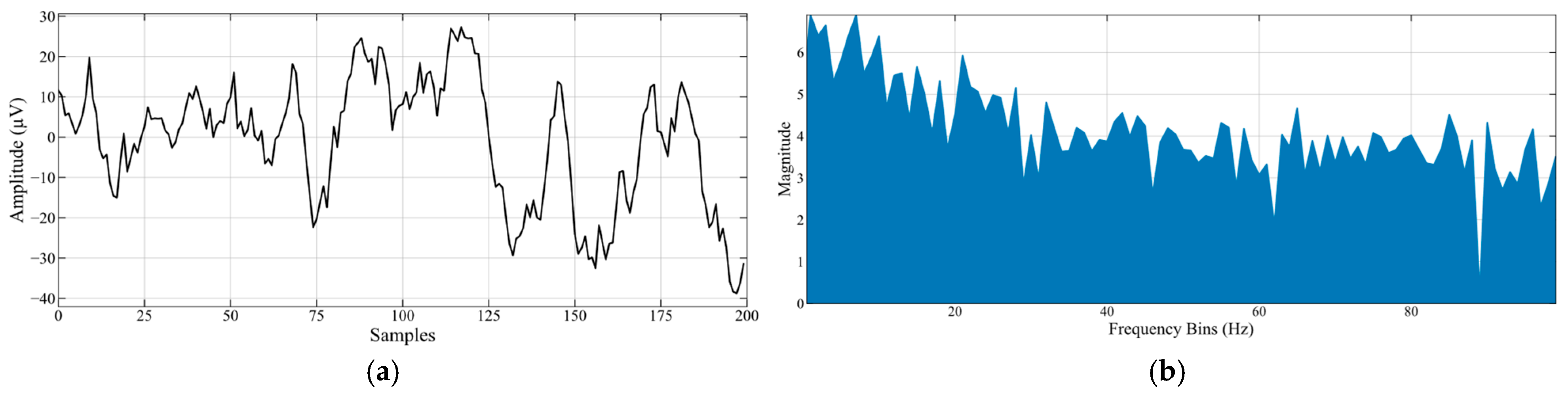
4.1.3. EEG Data Preprocessing

TUSZ employs two different referencing methods for EEG recordings, using two unipolar montages—Average Reference (AR) and Linked Ear Reference (LE). To ensure consistency, we selected 18 channel pairs that are common in every patient under both montages. For the CHB-MIT dataset, we chose 18 channel pairs shared across all patients. All EEG samples from both datasets were resampled to 200 Hz, then a 60 Hz Butterworth notch filter was applied to clean the signal from power-line artifacts. Figure 2 depicts a 1 s segment of a single-channel EEG after preprocessing. EEG clips were then extracted with a maximum sequence length of 30 s (30 s). Based on prior research as in [18], the raw EEG data was transformed using fast Fourier transform (FFT), then only the log-amplitude of the positive frequency components was retained, producing 100 features per EEG channel. FFT features effectively capture the spectral properties of EEG data, while representing them in the log-amplitude domain compresses extreme values and preserves the relative differences between amplitudes. This reduction in scale disparity enables neural networks to learn more effectively from the data. Figure 3b depicts the output of the FFT after the log transformation. The resulting data was then normalized using the mean and standard deviation of the training data. Finally, an EEG clip can be represented as $\mathit{X}\in {\mathbb{R}}^{T\times C\times F}$, where T = 30 denotes the clip length in seconds, C = 18 represents the number of EEG channels, and F = 100 represents the transformed FFT feature dimension.

4.1.4. Class Balancing, Data Splitting, and Evaluation Strategy

Since the data is highly imbalanced for both datasets as shown in Figure 3, we balance the number of samples for each class in the training set. Non-seizure samples are randomly down-sampled to match the number of seizure samples per session for each patient. In sessions with only non-seizure events, samples are randomly chosen based on the patient’s average seizure sample count per session. Validation and test sets include all available samples for the included patients, regardless of the class imbalance. This is performed to reflect real-world conditions, ensuring realistic model evaluation where seizure events are rare.

To further evaluate the model under conditions that reflect real-world scenarios, we use cross-patient evaluation, where models are trained, validated, and tested on distinct patients to measure the model’s performance on unseen patient data. For TUSZ, we follow the distinct patient-level splits provided in [18], with 527 patients used for training, 61 for validation, and 45 for testing. However, for CHB-MIT, we extend the experimental setup in [17] by employing a Leave-One-Patient-Out (LOPO) approach with validation splits for all of the 24 cases. In this cyclic setup, each fold reserves one patient’s data for testing, the preceding two patients for validation, and the remaining data for training. For example, the first fold will consist of the training data from patients chb02 to chb22, validation data from patients chb23 and chb24, and test data from patient chb01.

Table 1. Dataset summary for training, validation, and test splits.

Dataset	Split	Number of EEG Clips (Non-Seizure)	Number of EEG Clips (Seizure)
TUSZ	Training	6314	5853
	Validation	10,764	1058
	Test	16,671	1986
CHB-MIT	Training *	1386	1311
	Validation *	9687	124
	Test *	4843	62

* The values are the average number of samples across all folds for each class.

summarizes the number of patients and seizure events for both classes across both datasets.

4.2. Performance and Evaluation Metrics

Due to the highly imbalanced number of seizure samples per class in the test set, we adopted the evaluation metrics used in [17]. We use balanced accuracy (BA) which measures the average recall per class. In binary classification, balanced accuracy assigns equal weight to both sensitivity and specificity, helping to address class imbalance during evaluation. Sensitivity, or recall, measures the proportion of true positives correctly identified, while specificity measures the proportion of true negatives correctly identified. It offers a concise summary of a model’s performance on both positive and negative classes.

The Area Under the Receiver Operating Characteristic (AUROC) curve evaluates the discrimination ability across different thresholds by summarizing the ROC curve in a single metric. These thresholds are automatically defined in a data-driven manner using scikit-learn library [36]. The ROC curve quantifies the trade-off between the true positive rate (TPR) and false positive rate (FPR) across these thresholds. Additionally, we use the area under the precision–recall curve (AUPRC), which calculates the trade-off between the positive predictive value (PPV), or precision, and the TPR, or recall, across different thresholds, and summarizes the results in a single metric. Precision is the proportion of correctly identified positive cases among all samples predicted as positive. The AUPRC metric is especially useful when evaluating a model’s performance on imbalanced datasets, where seizure samples are scarce compared to abundant non-seizure samples.

Moreover, the non-linear dynamics of deep neural networks make their performance sensitive to a range of stochastic factors, including random-seed selection, weight-initialization methods, mini-batch data shuffling, regularization techniques like dropout, choice of optimization algorithm, learning rate schedule, and the timing of early stopping. To account for this variability and assess the statistical significance of deep learning models, we employ almost stochastic order (ASO) [37,38], as implemented in [39] using Bonferroni correction. The ASO statistic test evaluates whether a stochastic order exists between two models according to their score distributions across multiple runs with different random seeds. When comparing two models, A and B, the ASO test calculates a statistic ${\epsilon }_{min}$ that measures how model A outperforms model B across multiple runs. Given a significance level $\alpha \in (0, 1)$, an ${\epsilon }_{min}=0.0$ signifies that model A is stochastically dominant over model B. When ${\epsilon }_{min}<\tau$, where $\tau$ = 0.2, we can say model A is almost stochastically dominant over model B. The lower ${\epsilon }_{min}$ is, the higher the confidence to claim that model A outperforms model B. We set $\alpha =0.05$ (95% confidence interval) with bootstrap resampling of 5000 iterations.

4.3. Training Setup and Key Parameters

All models are trained with a batch size of 8, utilizing Adam optimizer with a cosine annealing learning rate scheduler [40]. The initial learning rate is 1 × 10⁻⁴ with a weight decay of 5 × 10⁻⁴ utilizing binary cross-entropy loss function followed by a sigmoid activation for binary classification. All models are trained for a maximum of 50 epochs, with early stopping of 5 epochs. The best performing model state is selected based on the highest BA score evaluated on the validation set. All models are run 5 times with different random seeds. The average results are then reported.

To optimize the GT-STAFG parameters and balance complexity with performance, we employed Bayesian optimization (BO) [41]. The BO search ends after exploring 5% of the search space or upon convergence, whichever comes first. Model parameters are chosen based on the highest BA performance on the validation set, with the final decision guided by the count of trainable parameters. The selected model results in 1,008,513 trainable parameters. For the baseline models, the default settings suggested by the authors are used.

Table 2. Hyperparameter ranges and optimal values for GT-STAFG.

Key Parameter	Value Range	Optimal Value
$\mathrm{Top} \mathrm{Neighbor} \mathrm{edges} \mathrm{per} \mathrm{node} (\tau$)	{2, 3, 4}	3
Hidden dimension size (d)	{64, 128, 256}	128
Spatial positional encoding (SPE)	{LPE, RWPE}	RWPE
Number of Random Walk steps	{3, 4, 5, 6}	4
Number of graph transformer layers	{1, 2, 4, 8}	4
Attention heads (H)/(P)	{4, 8, 16}	8/8
Number of FC layers (Classifier Head)	{1, 2, 3, 4}	2
Dropout probability (GT Layers)	{0.0, 0.1, 0.2}	0.2
Dropout probability (Classifier Head)	{0.0, 0.1, 0.2}	0.0

(H) is the number of attention heads per GT Layer. (P) is the number of attentions heads in STAFG.

summarizes the range of the explored hyperparameters, and the optimal values found, while

Table 3. The architecture of the GT-STAFG model.

Layer		Input Size	Output Size	Other Parameters
Input Layers	Node embedding	$\left(\text{\#}, \mathrm{T}, \mathrm{C}, 100\right)$	$\left(\text{\#}, \mathrm{T}, \mathrm{C}, 128\right)$	$-$
	Edge embedding	$\left(\text{\#}, \mathrm{T},\mathcal{E},\mathit{A}\right)$	$\left(\text{\#}, \mathrm{T},\mathcal{E},\mathit{A}, 128\right)$	$-$
Node Positional Encoding	TPE embedding	$\left(\mathrm{T}, \mathrm{C}, 128\right)$	$\left(\mathrm{T}, \mathrm{C}, 128\right)$	$-$
	SPE embedding	$\left(\text{\#}, \mathrm{T}, \mathrm{C}, 4\right)$	$\left(\text{\#},\mathrm{T}, \mathrm{C}, 128\right)$	$-$
Spatiotemporal Attention Fusion Gate (STAFG)	TPE attention module	$\left(\text{\#}, \mathrm{T}, \mathrm{C}, 128\right)$ ${\left(\mathrm{T}, \mathrm{C}, 128\right) }^{\text{†}}$	$\left(\text{\#}, \mathrm{T},\mathrm{C}, 128\right)$	$\mathrm{P}\text{:} 8$
	SPE attention module	$\left(\text{\#}, \mathrm{T}, \mathrm{C}, 128\right)$ ${\left(\text{\#}, \mathrm{T}, \mathrm{C}, 128\right)}^{ \text{†}}$	$\left(\text{\#}, \mathrm{T},\mathrm{C}, 128\right)$	$\mathrm{P}\text{:} 8$
	Fusion Gate	$\left(\text{\#}, \mathrm{T}, \mathrm{C}, 256\right)$	$\left(\text{\#}, \mathrm{T}, \mathrm{C}, 128\right)$	$-$
Graph Transformer (GT) Block	$\mathrm{GT} \mathrm{Layer} \times$ 4	$\left(\text{\#}, \mathrm{T}, \mathrm{C}, 128\right)$ $\left(\text{\#}, \mathrm{T}, \mathit{A},128\right)$	$\left(\text{\#}, \mathrm{T}, \mathrm{C}, 128\right)$ $\left(\text{\#}, \mathrm{T}, \mathit{A}, 128\right)$	$\mathrm{H}\text{:} 8$ $\mathrm{D}\text{:} 0.2$ $\mathrm{R}\text{:} \mathrm{GeLU}$
Graph Readout (mean)		$\left(\text{\#}, \mathrm{T}, \mathrm{C}, 128\right)$	$\left(\text{\#}, 128\right)$	$-$
Classifier Head	FC layer 1	$\left(\text{\#}, 128\right)$	$\left(\text{\#}, 128\right)$	$\mathrm{D}\text{:} 0.0$ $\mathrm{R}\text{:} \mathrm{GeLU}$
	FC layer 2	$\left(\text{\#}, 128\right)$	$\left(\text{\#}, 1\right)$	$-$

# is the batch size. ^† is the positional encoding embedding. D is the dropout probability rate; R is the activation function.

details the proposed GT-STAFG architecture.

Notably, RWPE was selected as an optimal SPE, as it can effectively capture how local regions of the EEG brain network evolve across time. Since seizures often involve bursts of synchronization or desynchronization, RWPE can exploit interconnected sub-graphs by focusing on local edge dynamics. This localization enables capturing finer temporal characteristics, allowing subtle changes in brain network dynamics to be detected. In contrast, LPE’s global graph representation reduces its discriminatory power due to the sparse connections (top-$\tau$ = 3) and small graph structure (18 nodes per graph). Additional experiments on the graph-based datasets reported in [42] verify our conclusion regarding RWPE.

5. Results and Discussion

In this section, we demonstrate that GT-STAFG consistently surpasses baseline models across multiple performance metrics. We also show that the proposed Spatiotemporal Attention Fusion Gate outperforms classical fusion strategies. We use Integrated Gradients to visualize features that align with clinically relevant EEG patterns. Finally, we conduct transfer learning experiments to explore the model’s performance in a domain-shift scenario.

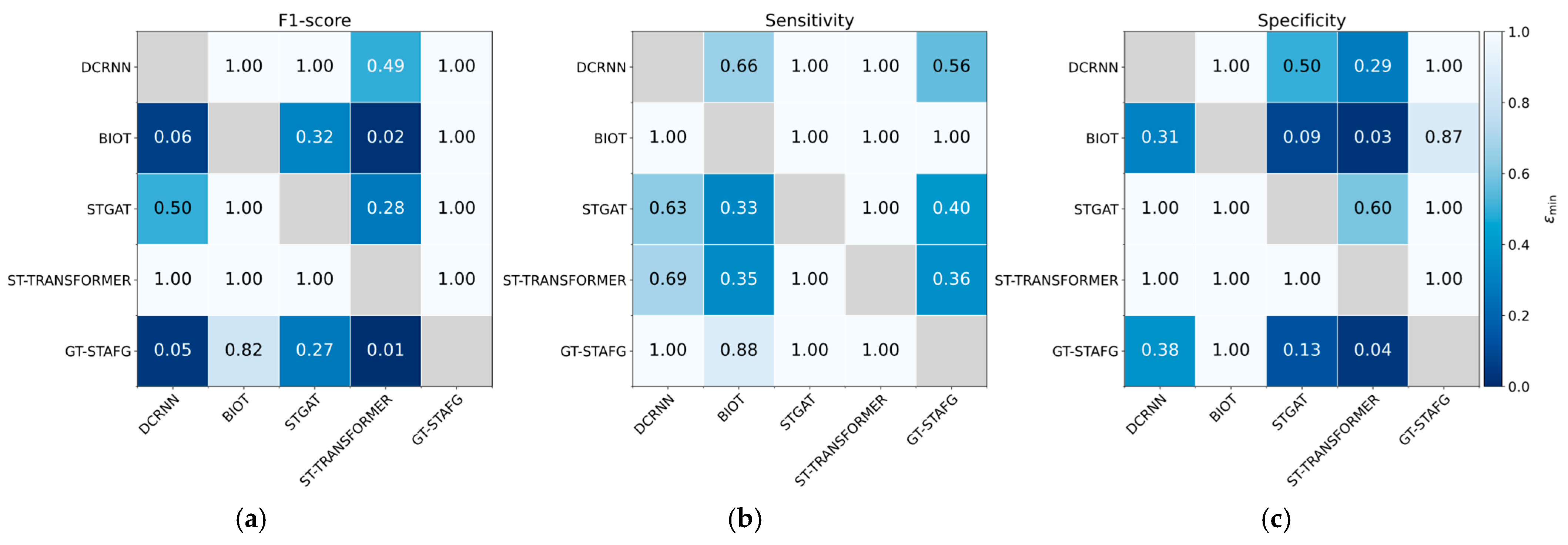
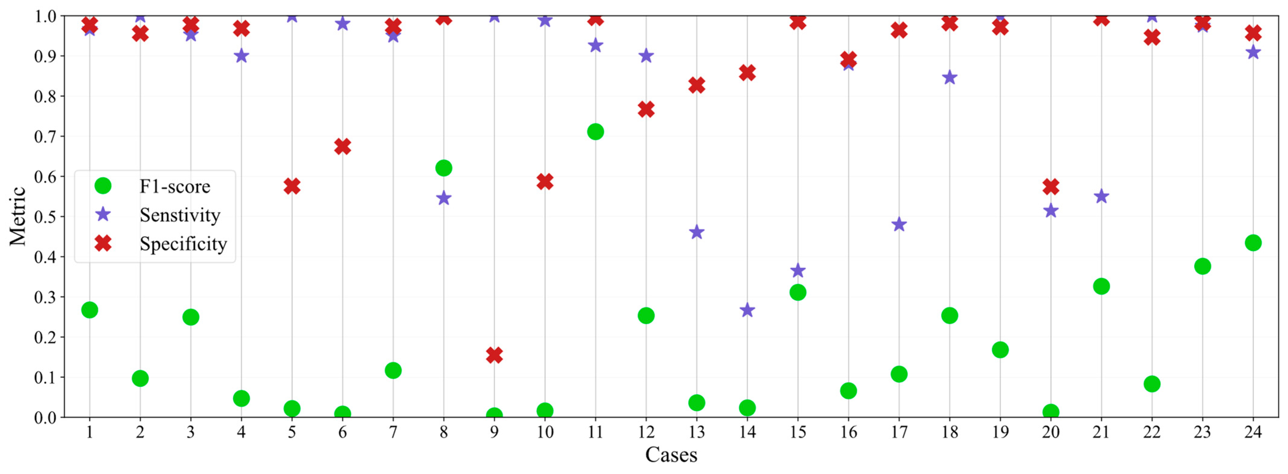
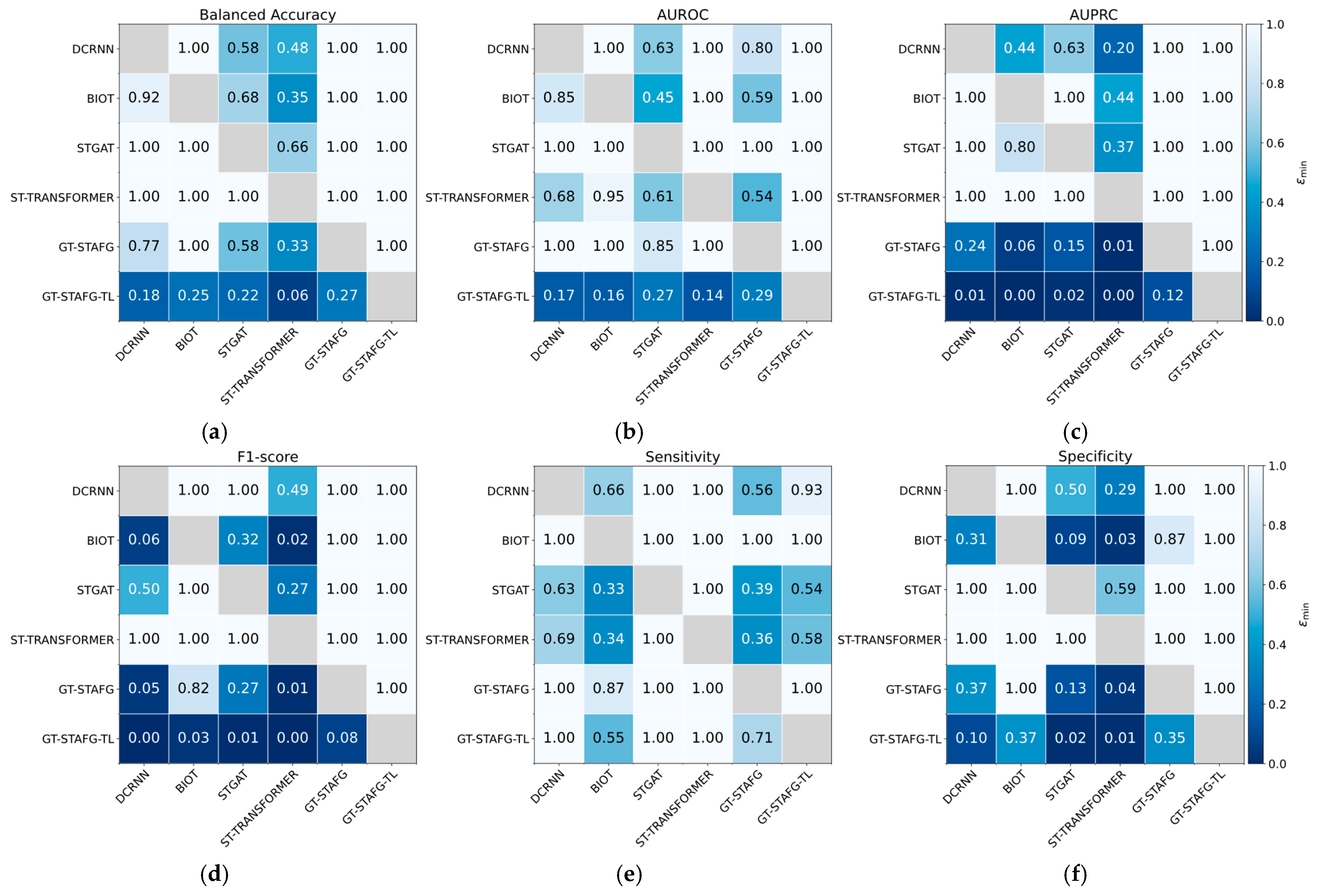
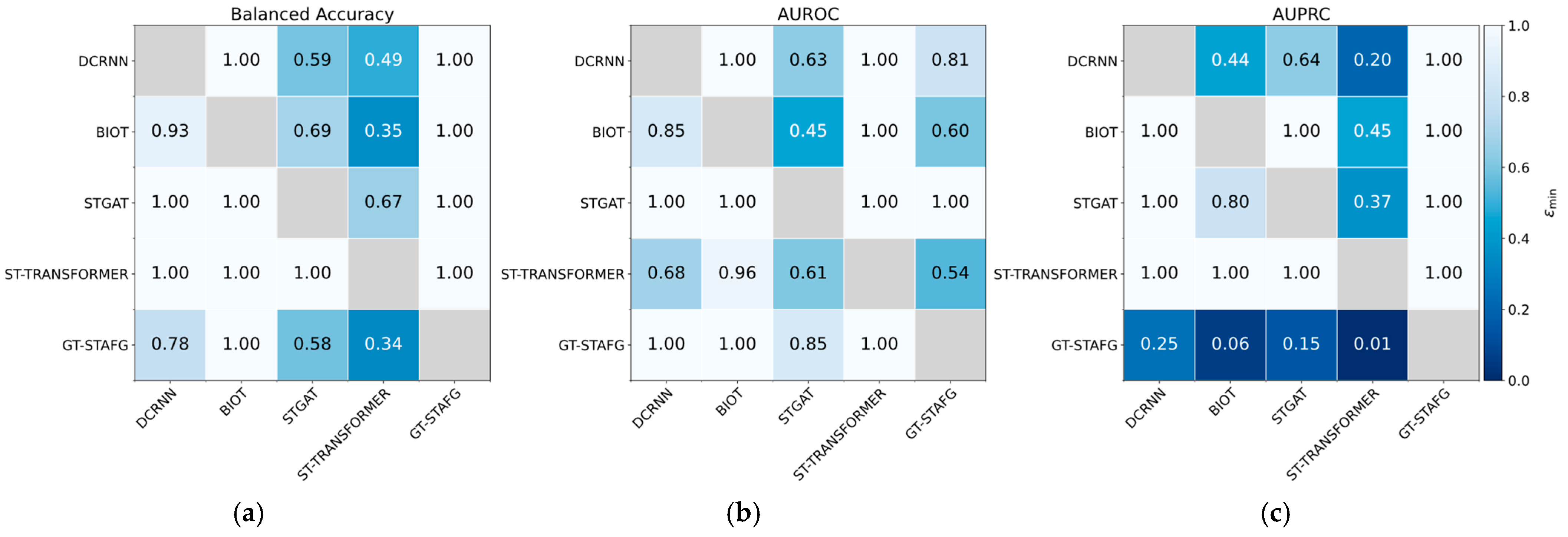
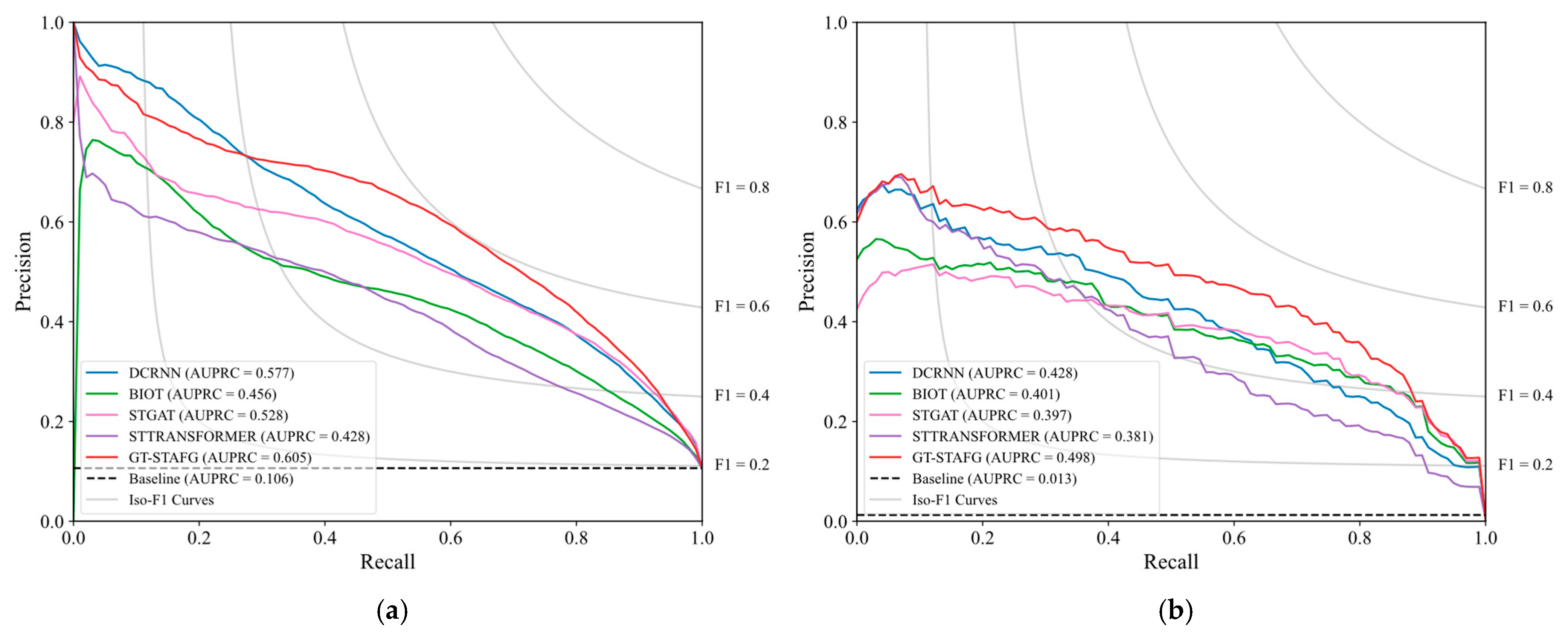
5.1. Performance Compared to Baselines

The proposed GT-STAFG model is compared to four end-to-end deep learning models. These models are DCRNN [18], BIOT [17], STGAT [23], and ST-TRANSFORMER [16]. DCRNN integrates graph convolution within GRU units, STGAT combines graph attention with GRU, while BIOT and ST-TRANSFORMER leverage transformer architectures with different spatial encoding strategies.

Table 4. Performance metrics (mean ± std) of various baseline models for TUSZ and CHB-MIT datasets compared to the proposed GT-STAFG.

Model	TUSZ			CHB-MIT
	BA	AUROC	AUPRC	BA	AUROC	AUPRC
DCRNN	0.820 ± 0.003	0.899 ± 0.003	0.577 ± 0.023	0.819 ± 0.027	0.918 ± 0.023	0.428 ± 0.054
BIOT	0.784 ± 0.008	0.864 ± 0.006	0.456 ± 0.030	0.827 ± 0.025	0.924 ± 0.020	0.387 ± 0.050
STGAT	0.818 ± 0.015	0.899 ± 0.008	0.528 ± 0.028	0.810 ± 0.029	0.914 ± 0.028	0.397 ± 0.059
ST-TRANSFORMER	0.757 ± 0.008	0.847 ± 0.003	0.428 ± 0.025	0.797 ±0.027	0.919 ± 0.017	0.351 ± 0.041
GT-STAFG (proposed)	0.835 ± 0.009	0.911 ± 0.004	0.605 ± 0.013	0.831 ± 0.028	0.921 ± 0.027	0.498 ± 0.045

presents the performance of the proposed GT-STAFG model with other baseline models across the TUSZ and CHB-MIT datasets using the aforementioned performance metrics. For each metric, the best performance is highlighted in bold, while the second-best is underlined. The standard baseline for threshold-specific metrics such as balanced accuracy is 0.5. Refer to Appendix B.1 for additional performance metrics scores.

On the TUSZ dataset, GT-STAFG demonstrates robust performance, surpassing all baselines across all metrics. Although the performance difference between DCRNN, the overall second-best, is marginal for BA (1.5 percentage points) and AUROC (1.2 percentage points), GT-STAFG surpasses DCRNN by 2.8 percentage points in AUPRC. This indicates that GT-STAFG is better at accurately identifying true positive instances in highly imbalanced datasets. Consequently, fewer missed seizures and false alarms improve patient outcomes, as timely intervention becomes more likely and healthcare providers gain greater trust in the model, reducing unnecessary clinical workload. It is important to note that both balanced accuracy (BA) and AUROC are not considered the most reliable metrics for measuring performance in imbalanced datasets. Although balanced accuracy accounts for the minority class, high specificity can mask poor recall performance, making it less discriminative for seizure detection. Similarly, although AUROC is widely used for binary classification tasks, it can give an overly optimistic performance in highly imbalanced datasets, since the abundance of negative samples keeps the false positive rate low [43]. In contrast, AUPRC provides a more clinically meaningful assessment, as it focuses exclusively on the model’s ability to correctly identify seizure instances without being affected by the abundance of non-seizure samples. On the CHB-MIT dataset, GT-STAFG shows the best performance across most of the metrics. Although it marginally surpasses DCRNN and BIOT in BA by 1.2 and 0.4 percentage points, respectively, it demonstrates superior performance in AUPRC, exceeding DCRNN and BIOT by a substantial margin of 7.0 and 11.1 percentage points, respectively. Again, this reflects GT-STAFG’s high sensitivity in detecting rare seizure events across various detection thresholds. Although GT-STAFG is ranked second in AUROC, all models performed similarly, within the range of 1.0 percentage points’ difference between the best performer (BIOT) and the poorest performer (STGAT).

Figure 4 and Figure 5 present the ASO statistic test for balanced accuracy, AUROC, and AUPRC metrics for all models across TUSZ and CHB-MIT datasets, respectively. In Figure 4, it is evident that GT-STAFG almost stochastically dominates all baseline models in these performance metrics for the TUSZ dataset. In Figure 5, no dominance is seen in both balanced accuracy and AUROC metrics, which aligns with the results observed in Table 4, where a significant overlap exists in both of these metrics scores across all models. In contrast, GT-STAFG almost stochastically dominates every baseline in the AUPRC metric, except for DCRNN which presents the least level of confidence $\left({ϵ}_{min}=0.25\right)$.

Figure 6 illustrates the area under the precision–recall curve for the proposed model, GT-STAFG, along with baseline models evaluated on both the TUSZ and CHB-MIT datasets. The curves clearly highlight GT-STAFG’s comparative advantage in imbalanced scenarios. With proper detection threshold fine-tuning, GT-STAFG can deliver superior performance compared to the other baseline models. Remarkably, AUPRC on CHB-MIT dataset remains lower than on TUSZ, suggesting persistent challenges in capturing rare seizure events due to high class imbalance [44], since the class imbalance in CHB-MIT is more severe compared to TUSZ. This performance discrepancy between datasets is observed across all models. However, graph-based models, such as GT-STAFG and DCRNN, have demonstrated robustness, achieving the top two AUPRC scores on both datasets. Notably, GT-STAFG consistently tops the AUPRC score, reflecting greater diagnostic confidence with fewer false positive rates.

To assess the cross-patient generalization performance of our proposed model on the CHB-MIT dataset, we evaluate GT-STAFG’s performance by conducting Leave-One-Patient-Out (LOPO) with validation splits across the 24 cases. As shown in Figure 7, most cases show high BA performance, while reaching near-perfect or perfect scores for AUROC, except for patients #5 and #11. These patients may reflect patient-specific variability, with their rare seizure patterns absent from the training data [44]. Remarkably, the performance of AUPRC for most cases is considered relatively low. This observation implies two important aspects. First, it emphasizes the high imbalance between seizure and non-seizure samples. Second, case-by-case AURPC values vary significantly, indicating that the model’s precision is very low for certain patients due to significant inter-subject variability [44]. This pattern suggests the need for per-subject threshold calibration. Overall, these results highlight GT-STAFG’s clinical promise as it delivers high seizure detection performance while keeping false alarms low. Additionally, its robust cross-patient performance suggests it can reduce the burden of manual EEG review. Refer to Appendix B.2 for additional performance metrics scores.

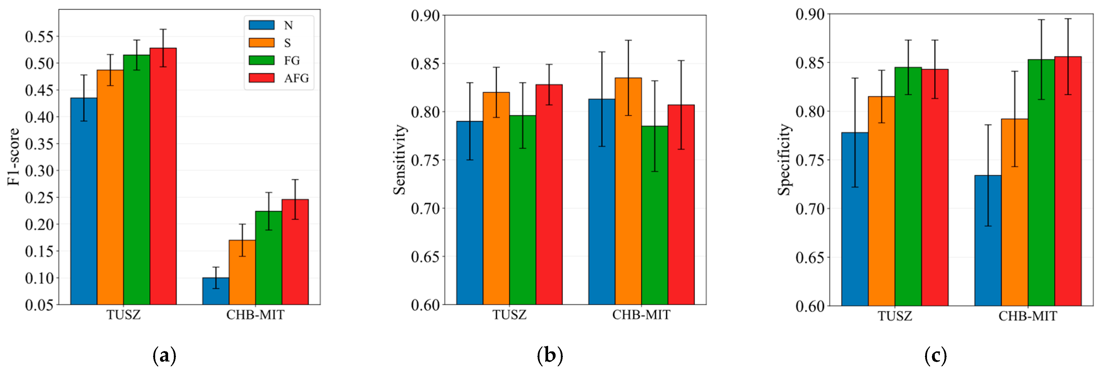
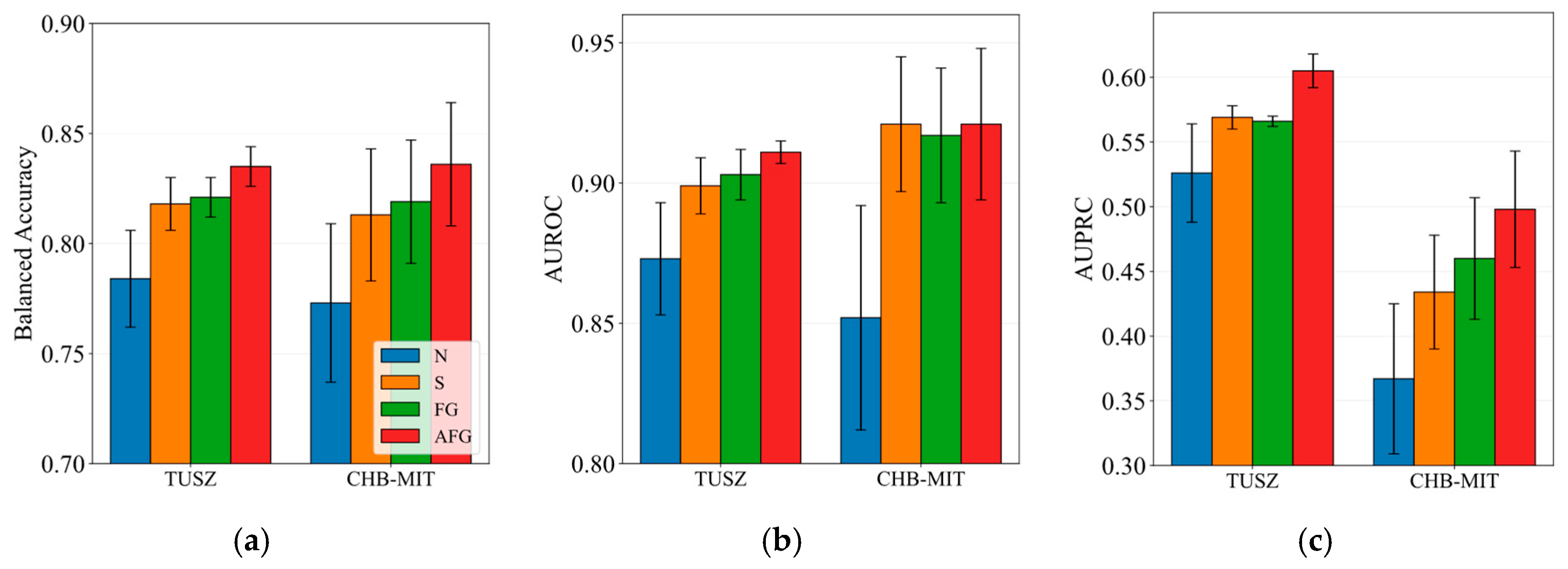
5.2. Impact of Spatiotemporal Attention Fusion Gate

To demonstrate the effectiveness of the proposed technique with the graph transformer, we compare it to classical positional encoding combination techniques from [17,31]. We evaluate the different scenarios according to the following configurations outlined in

Table 5. Different techniques for the positional encodings using graph transformer.

Technique	Description
N	No positional encodings are used.
S	Spatial and temporal positional encodings are directly added to the node embeddings.
FG	Spatial and temporal positional encodings are fused via a fusion gate, then added to the node embeddings.
AFG (proposed)	Spatial and temporal positional encodings are separately added to the node embeddings, processed by separate attention mechanisms, fused via a fusion gate, and combined with original node embeddings via a residual connection.

. The proposed attention fusion gate technique is referred to as (AFG). Since hyperparameter tuning selected RWPE as optimal, we use it as the spatial positional encoding (SPE) across all techniques. All the approaches have the same setting as detailed in Section 4.3. Figure 8 compares the proposed attention fusion gate (AFG) to the techniques in Table 5, with (N) as a baseline reference. (AFG) achieves the highest performance across both TUSZ and CHB-MIT datasets, except for AUROC on CHB-MIT, where (S) performs similarly. For AUPRC, AFG shows statistically significant gains over all other methods on TUSZ and comparably higher performance on CHB-MIT. Error bars indicate low variance across independent runs, highlighting the consistency of (AFG). The AUPRC gains demonstrate superior positive-predictive power in across both datasets, which is considered a critical factor for reducing false alarms in clinical practice. Moreover, AFG’s strong performance across both datasets emphasizes its robustness and adaptability to different patient populations. Compared to (N), (S), and (FG), the proposed (AFG) enriches node features with dynamic spatial and temporal information, enabling more effective integration of positional encodings. Refer to Appendix B.3 for additional performance metrics scores.

5.3. Feature Attribution and Clinical Practicality

As previously mentioned, visualizing influential frequency features offers insights into the underlying patterns driving deep learning model predictions, enhancing model transparency and holding potential for clinical applications. Figure 9 presents the IG scores of a sample’s input FFT features, the predictions of the proposed model compared to ground truth annotations for each segment, and a single channel from the original time-domain EEG signal. The intuition for positive IG scores is that a feature’s deviation from the baseline pushes the prediction toward a seizure class, while negative IG scores indicate the opposite. Since a baseline is required for computing IG scores, a zero-scaled vector is used, representing the average of all normalized training samples.

As shown in Figure 9a, elevated IG scores reveal two regions of interest. The first region spans approximately from 1 to 5 Hz, suggesting it aligns with the delta band. The second region extends roughly from 11 to 16 Hz, which aligns with low beta band frequencies [45]. For the first region associated with the delta band, the attributions shifted from negative to positive during seizure events, indicating that these frequencies serve as critical biomarkers guiding the model’s decisions towards seizure detection. This observation is consistent with literature that highlights increased delta power during seizure activity [46]. Furthermore, it can be observed that within the 1 to 5 Hz range, the highest positive attribution occurs at 3 Hz, which may correlate with absence seizures. This type of seizure can be usually identified through their characteristic 3 Hz spike–wave complexes (SWCs) [47]. Nevertheless, since the scope of this work is seizure detection rather than seizure type classification, the current work may be extended in the future to differentiate between different types of seizures. For the second region, associated with lower beta band frequencies (beta-1), positive attributions are already present during non-seizure states; however, these positive attributions appear to be higher during seizures. One possible interpretation is that this patient’s beta activity is normally higher than the average; thus, the consistently positive attributions during non-seizure events reflect an elevated baseline rather than an indication of seizure activity. In contrast, the additional increase in positive attributions during seizures may be a direct result of the seizure itself.

Figure 9b illustrates the predictions of the proposed model compared to the manually annotated expert labels. The model successfully detects all seizure segments with near-perfect accuracy. For non-seizure segments, most predictions fall below the detection threshold (0.5) by a reasonable margin. Interestingly, some of the segments preceding the seizure events show a higher prediction probability, compared to preceding non-seizure segments, with only one event falsely identified as a seizure. This indicates that the model may have the ability to detect subtle pre-seizure activity. Although detecting these patterns looks promising, further exploration of these patterns is beyond the scope of this work. In conclusion, by attributing specific frequency features, the Integrated Gradients method identifies which frequencies are influential in detecting epileptic seizures. This insight offers clinicians a clearer understanding of the model’s decision-making process and builds trust between clinicians and artificial intelligence-based tools.

5.4. Transfer Learning

Machine learning often assumes similar distributions between source and target data, which is not true for TUSZ and CHB-MIT datasets. TUSZ covers diverse age groups, while CHB-MIT focuses on pediatric patients. This discrepancy could lead to poor cross-performance. Training from scratch could be impractical due to limited resources and scarce labels. Herein, transfer learning (TL) solves this by leveraging the knowledge from one dataset to improve performance on the other [48].

We perform transfer learning by fine-tuning the models pre-trained on the TUSZ dataset using the CHB-MIT dataset. Transferring from CHB-MIT to TUSZ was not performed due to the small number of patients and scarce seizure events in CHB-MIT. The learning rate of fine-tuning process was set to 5 × 10⁻⁵ with cosine annealing scheduler for 25 epochs, allowing the model to adapt to the patients’ features in the CHB-MIT dataset, while preserving generalizable features from the pretrained weights of TUSZ patients. The rest of the training setup remains the same as detailed in Section 4.3.

Table 6. Transfer learning performance metrics from TUSZ to CHB-MIT.

BA	AUROC	AUPRC
0.860 ± 0.022 (+0.029) †	0.955 ± 0.015 (+0.034) †	0.581 ± 0.041 (+0.083) †

^† The result represents the performance gain achieved through transfer learning compared to training the model from scratch.

presents the performance of the fine-tuned models via transfer learning compared to training from scratch. The fine-tuned models consistently outperform the scratch-trained models across all performance metrics. Remarkably, the fine-tuning process significantly enhanced performance, improving AUPRC on average by 8.3 percentage points, with BA and AUROC also showing gains of 2.9 and 3.4 percentage points, respectively. These results demonstrate GT-STAFG’s capacity to effectively enhance its performance on highly imbalanced datasets such as CHB-MIT. Overall, the findings indicate that the proposed model has learned generalizable features from the TUSZ dataset, leading to enhanced seizure detection performance on the CHB-MIT dataset. Refer to Appendix B.4 for additional performance metrics scores and ASO statistic test results for GT-STAFG transfer-learning variant.

Figure 10 illustrates the performance differences of GT-STAFG after applying transfer learning across all 24 cases in the CHB-MIT dataset. Overall, transfer learning improved performance for most cases, particularly cases #16 and #17 where initial performance across all metrics was very low. However, a subset of patients experienced varying degrees of performance decline, especially cases #5 and #8, which experienced the highest drop in AUPRC. This drop suggests that certain patient-specific patterns might limit the effectiveness of the transfer learning approach applied. Given the scope of the current work, we have not analyzed these individual cases in depth. Future research will aim to identify the underlying reasons for these declines, potentially leading to more personalized model adjustments.

6. Conclusions

In this work, we present a Graph Transformer with a Spatiotemporal Attention Fusion Gate (GT-STAFG) for efficient and improved seizure detection in EEG data. The proposed method enhances performance and improves EEG features learning by overcoming the limitations in traditional cascaded spatial–temporal feature processing, which restricts the interaction between spatial and temporal features, limiting deeper contextual learning. By enhancing the EEG feature representation, GT-STAFG enables richer feature learning and achieves robust performance. Experimental results show that GT-STAFG outperforms four baseline models across two datasets, TUSZ and CHB-MIT. Moreover, combining the Attention Fusion Gate with the Graph Transformer delivers superior performance compared to other positional encoding combination techniques.

Transfer learning from the TUSZ to the CHB-MIT dataset further emphasizes the model’s potential for improved cross-patient generalization, enhancing its promise in diverse clinical settings across multiple patient cases. Nevertheless, the demonstrated model’s performance relies on consistent EEG data, and variations in data collection or missing data may affect its real-world use. Moreover, the Integrated Gradients (IGs) attribution method demonstrates that the delta sub-band frequency is key for identifying seizures and provides interpretable insights into the model’s decision-making process, which is crucial for clinical translation. However, the analysis in this work is limited to interpreting the direct effects of individual frequency sub-bands without exploring their interactions which might affect the interpretability of the IG scores.

Overall, GT-STAFG shows robust cross-patient performance in seizure detection. This advancement can streamline clinical workflows by reducing manual reviews, alleviating the burden on clinical resources and improving patient outcomes. In the future, we plan to focus our research on the following directions:

• Examine the model’s performance across a range of detection thresholds to find the optimal threshold that aligns with the practical clinical deployment needs.
• Investigate the performance of GT-STAFG on noisy and incomplete EEG data, such as missing and noisy EEG channels.
• Explore Integrated Gradient feature interactions to assess frequency band influence on seizure detection.
• Improve the performance of the transfer learning application.
• Extend the study for seizure type classification and on additional datasets.

References

1. Nafea, M.S.; Ismail, Z.H. Supervised Machine Learning and Deep Learning Techniques for Epileptic Seizure Recognition Using EEG Signals: A Systematic Literature Review. Bioengineering 2022, 9, 781. [Google Scholar] [CrossRef]
2. Saab, K.; Dunnmon, J.; Ré, C.; Rubin, D.; Lee-Messer, C. Weak Supervision as an Efficient Approach for Automated Seizure Detection in Electroencephalography. NPJ Digit. Med. 2020, 3, 59. [Google Scholar] [CrossRef]
3. Sinha, S.R.; Sullivan, L.; Sabau, D.; San-Juan, D.; Dombrowski, K.E.; Halford, J.J.; Hani, A.J.; Drislane, F.W.; Stecker, M.M. American Clinical Neurophysiology Society Guideline 1: Minimum Technical Requirements for Performing Clinical Electroencephalography. J. Clin. Neurophysiol. 2016, 33, 303–307. [Google Scholar] [CrossRef] [PubMed]
4. Shoeibi, A.; Khodatars, M.; Ghassemi, N.; Jafari, M.; Moridian, P.; Alizadehsani, R.; Panahiazar, M.; Khozeimeh, F.; Zare, A.; Hosseini-Nejad, H.; et al. Epileptic Seizures Detection Using Deep Learning Techniques: A Review. Int. J. Environ. Res. Public Health 2021, 18, 5780. [Google Scholar] [CrossRef] [PubMed]
5. Li, R.; Yuan, X.; Radfar, M.; Marendy, P.; Ni, W.; O’Brien, T.J.; Casillas-Espinosa, P. Graph Signal Processing, Graph Neural Network and Graph Learning on Biological Data: A Systematic Review. IEEE Rev. Biomed. Eng. 2023, 16, 109–135. [Google Scholar] [CrossRef] [PubMed]
6. Cong, S.; Wang, H.; Zhou, Y.; Wang, Z.; Yao, X.; Yang, C. Comprehensive Review of Transformer-based Models in Neuroscience, Neurology, and Psychiatry. Brain-X 2024, 2, e57. [Google Scholar] [CrossRef]
7. Craik, A.; He, Y.; Contreras-Vidal, J.L. Deep Learning for Electroencephalogram (EEG) Classification Tasks: A Review. J. Neural Eng. 2019, 16, 031001. [Google Scholar] [CrossRef]
8. Klepl, D.; Wu, M.; He, F. Graph Neural Network-Based EEG Classification: A Survey. IEEE Trans. Neural Syst. Rehabil. Eng. 2024, 32, 493–503. [Google Scholar] [CrossRef]
9. Jang, S.; Moon, S.-E.; Lee, J.S. EEG-Based Video Identification Using Graph Signal Modeling and Graph Convolutional Neural Network. In Proceedings of the 2018 IEEE International Conference on Acoustics, Speech and Signal Processing (ICASSP), Calgary, AB, Canada, 15–20 April 2018; pp. 3066–3070. [Google Scholar]
10. Veličković, P.; Casanova, A.; Liò, P.; Cucurull, G.; Romero, A.; Bengio, Y. Graph Attention Networks. In Proceedings of the 6th International Conference on Learning Representations, ICLR 2018—Conference Track Proceedings, Vancouver, BC, Canada, 30 April–3 May 2018; pp. 1–12. [Google Scholar]
11. Dwivedi, V.P.; Bresson, X. A Generalization of Transformer Networks to Graphs. arXiv 2020, arXiv:2012.09699. [Google Scholar]
12. Ye, Z.; Kumar, Y.J.; Sing, G.O.; Song, F.; Wang, J. A Comprehensive Survey of Graph Neural Networks for Knowledge Graphs. IEEE Access 2022, 10, 75729–75741. [Google Scholar] [CrossRef]
13. He, J.; Cui, J.; Zhao, Y.; Zhang, G.; Xue, M.; Chu, D. Spatial-Temporal Seizure Detection with Graph Attention Network and Bi-Directional LSTM Architecture. Biomed. Signal Process Control 2022, 78, 103908. [Google Scholar] [CrossRef]
14. Shan, X.; Cao, J.; Huo, S.; Chen, L.; Sarrigiannis, P.G.; Zhao, Y. Spatial–Temporal Graph Convolutional Network for Alzheimer Classification Based on Brain Functional Connectivity Imaging of Electroencephalogram. Hum. Brain Mapp. 2022, 43, 5194–5209. [Google Scholar] [CrossRef] [PubMed]
15. Vaswani, A.; Shazeer, N.; Parmar, N.; Uszkoreit, J.; Jones, L.; Gomez, A.N.; Kaiser, Ł.; Polosukhin, I. Attention Is All You Need. In Proceedings of the Advances in Neural Information Processing Systems, Long Beach, CA, USA, 4–9 December 2017; pp. 5999–6009. [Google Scholar]
16. Li, Q.; Zhang, T.; Song, Y.; Sun, M. Transformer-Based Spatial-Temporal Feature Learning for P300. In Proceedings of the 2022 16th ICME International Conference on Complex Medical Engineering, CME 2022, Zhongshan, China, 4–6 November 2022; pp. 310–313. [Google Scholar]
17. Yang, C.; Brandon Westover, M.; Sun, J. BIOT: Biosignal Transformer for Cross-Data Learning in the Wild. Adv. Neural Inf. Process Syst. 2023, 36, 78240–78260. [Google Scholar]
18. Tang, S.; Dunnmon, J.A.; Saab, K.; Zhang, X.; Huang, Q.; Dubost, F.; Rubin, D.L.; Lee-Messer, C. Self-Supervised Graph Neural Networks for Improved Electroencephalographic Seizure Analysis. In Proceedings of the International Conference on Learning Representations, Virtual, 25–29 April 2022. [Google Scholar]
19. Tian, X.; Jin, Y.; Zhang, Z.; Liu, P.; Tang, X. Spatial-Temporal Graph Transformer Network for Skeleton-Based Temporal Action Segmentation. Multimed. Tools Appl. 2023, 83, 44273–44297. [Google Scholar] [CrossRef]
20. Li, Y.; Liu, Y.; Cui, W.G.; Guo, Y.Z.; Huang, H.; Hu, Z.Y. Epileptic Seizure Detection in EEG Signals Using a Unified Temporal-Spectral Squeeze-and-Excitation Network. IEEE Trans. Neural Syst. Rehabil. Eng. 2020, 28, 782–794. [Google Scholar] [CrossRef]
21. Peng, R.; Zhao, C.; Jiang, J.; Kuang, G.; Cui, Y.; Xu, Y.; Du, H.; Shao, J.; Wu, D. TIE-EEGNet: Temporal Information Enhanced EEGNet for Seizure Subtype Classification. IEEE Trans. Neural Syst. Rehabil. Eng. 2022, 30, 2567–2576. [Google Scholar] [CrossRef]
22. Thuwajit, P.; Rangpong, P.; Sawangjai, P.; Autthasan, P.; Chaisaen, R.; Banluesombatkul, N.; Boonchit, P.; Tatsaringkansakul, N.; Sudhawiyangkul, T.; Wilaiprasitporn, T. EEGWaveNet: Multiscale CNN-Based Spatiotemporal Feature Extraction for EEG Seizure Detection. IEEE Trans. Industr Inform. 2022, 18, 5547–5557. [Google Scholar] [CrossRef]
23. Wang, Y.; Shi, Y.; Cheng, Y.; He, Z.; Wei, X.; Chen, Z.; Zhou, Y. A Spatiotemporal Graph Attention Network Based on Synchronization for Epileptic Seizure Prediction. IEEE J. Biomed. Health Inform. 2023, 27, 900–911. [Google Scholar] [CrossRef]
24. Feng, L.; Cheng, C.; Zhao, M.; Deng, H.; Zhang, Y. EEG-Based Emotion Recognition Using Spatial-Temporal Graph Convolutional LSTM with Attention Mechanism. IEEE J. Biomed. Health Inform. 2022, 26, 5406–5417. [Google Scholar] [CrossRef]
25. Wang, Z.; Wang, Y.; Hu, C.; Yin, Z.; Song, Y. Transformers for EEG-Based Emotion Recognition: A Hierarchical Spatial Information Learning Model. IEEE Sens. J. 2022, 22, 4359–4368. [Google Scholar] [CrossRef]
26. Wan, Z.; Li, M.; Liu, S.; Huang, J.; Tan, H.; Duan, W. EEGformer: A Transformer–Based Brain Activity Classification Method Using EEG Signal. Front. Neurosci. 2023, 17, 1148855. [Google Scholar] [CrossRef]
27. Zhao, W.; Jiang, X.; Zhang, B.; Xiao, S.; Weng, S. CTNet: A Convolutional Transformer Network for EEG-Based Motor Imagery Classification. Sci. Rep. 2024, 14, 20237. [Google Scholar] [CrossRef]
28. Lawhern, V.J.; Solon, A.J.; Waytowich, N.R.; Gordon, S.M.; Hung, C.P.; Lance, B.J. EEGNet: A Compact Convolutional Neural Network for EEG-Based Brain–Computer Interfaces. J. Neural Eng. 2018, 15, 56013. [Google Scholar] [CrossRef] [PubMed]
29. Xiang, J.; Li, Y.; Wu, X.; Dong, Y.; Wen, X.; Niu, Y. Synchronization-Based Graph Spatio-Temporal Attention Network for Seizure Prediction. Sci. Rep. 2025, 15, 4080. [Google Scholar] [CrossRef] [PubMed]
30. Dwivedi, V.P.; Luu, A.T.; Laurent, T.; Bengio, Y.; Bresson, X. Graph Neural Networks With Learnable Structural and Positional Representations. In Proceedings of the ICLR 2022—10th International Conference on Learning Representations, Virtual, 25–29 April 2022. [Google Scholar]
31. Arevalo, J.; Solorio, T.; Montes-Y-Gómez, M.; González, F.A. Gated Multimodal Units for Information Fusion. In Proceedings of the 5th International Conference on Learning Representations, ICLR 2017—Workshop Track Proceedings, Toulon, France, 24–26 April 2017. [Google Scholar]
32. Hendrycks, D.; Gimpel, K. Gaussian Error Linear Units (GELUs). arXiv 2016, arXiv:1606.08415. [Google Scholar]
33. Sundararajan, M.; Taly, A.; Yan, Q. (Integrated Gradient) Axiomatic Attribution for Deep Networks. In Proceedings of the 34th International Conference on Machine Learning, ICML 2017, Sydney, Australia, 6–11 August 2017; Volume 7, pp. 5109–5118. [Google Scholar]
34. Shah, V.; von Weltin, E.; Lopez, S.; McHugh, J.R.; Veloso, L.; Golmohammadi, M.; Obeid, I.; Picone, J. The Temple University Hospital Seizure Detection Corpus. Front. Neuroinform. 2018, 12, 83. [Google Scholar] [CrossRef]
35. Shoeb, A.; Guttag, J. CHB-MIT Dataset. In Proceedings of the ICML 2010—Proceedings, 27th International Conference on Machine Learning, Haifa, Israel, 21–24 June 2010; pp. 975–982. [Google Scholar]
36. Pedregosa, F.; Varoquaux, G.; Gramfort, A.; Michel, V.; Thirion, B.; Grisel, O.; Blondel, M.; Prettenhofer, P.; Weiss, R.; Dubourg, V.; et al. Scikit-Learn: Machine Learning in Python. J. Mach. Learn. Res. 2011, 12, 2825–2830. [Google Scholar]
37. Del Barrio, E.; Cuesta-Albertos, J.A.; Matrán, C. An Optimal Transportation Approach for Assessing Almost Stochastic Order BT—The Mathematics of the Uncertain: A Tribute to Pedro Gil; Gil, E., Gil, E., Gil, J., Gil, M.Á., Eds.; Springer International Publishing: Cham, Switzerland, 2018; pp. 33–44. ISBN 978-3-319-73848-2. [Google Scholar]
38. Dror, R.; Shlomov, S.; Reichart, R. Deep Dominance—How to Properly Compare Deep Neural Models. In Proceedings of the ACL 2019—57th Annual Meeting of the Association for Computational Linguistics, Proceedings of the Conference, Florence, Italy, 28 July–2 August 2019; pp. 2773–2785. [Google Scholar]
39. Ulmer, D.; Hardmeier, C.; Frellsen, J. Deep-Significance—Easy and Meaningful Statistical Significance Testing in the Age of Neural Networks. arXiv 2022, arXiv:2204.06815. [Google Scholar]
40. Loshchilov, I.; Hutter, F. SGDR: Stochastic Gradient Descent with Warm Restarts. In Proceedings of the International Conference on Learning Representations, Toulon, France, 24–26 April 2017. [Google Scholar]
41. Snoek, J.; Larochelle, H.; Adams, R.P. Practical Bayesian Optimization of Machine Learning Algorithms. Adv. Neural Inf. Process Syst. 2012, 4, 2951–2959. [Google Scholar]
42. Rampášek, L.; Galkin, M.; Dwivedi, V.P.; Luu, A.T.; Wolf, G.; Beaini, D. Recipe for a General, Powerful, Scalable Graph Transformer. In Proceedings of the Advances in Neural Information Processing Systems, New Orleans, LA, USA, 28 November–9 December 2022; Volume 35. [Google Scholar]
43. Saito, T.; Rehmsmeier, M. The Precision-Recall Plot Is More Informative than the ROC Plot When Evaluating Binary Classifiers on Imbalanced Datasets. PLoS ONE 2015, 10, e0118432. [Google Scholar] [CrossRef]
44. Ali, E.; Angelova, M.; Karmakar, C. Epileptic Seizure Detection Using CHB-MIT Dataset: The Overlooked Perspectives. R. Soc. Open Sci. 2024, 11, 230601. [Google Scholar] [CrossRef] [PubMed]
45. Weiss, S.; Mueller, H.M. “Too Many Betas Do Not Spoil the Broth”: The Role of Beta Brain Oscillations in Language Processing. Front. Psychol. 2012, 3, 201. [Google Scholar] [CrossRef] [PubMed]
46. De Stefano, P.; Carboni, M.; Marquis, R.; Spinelli, L.; Seeck, M.; Vulliemoz, S. Increased Delta Power as a Scalp Marker of Epileptic Activity: A Simultaneous Scalp and Intracranial Electroencephalography Study. Eur. J. Neurol. 2022, 29, 26–35. [Google Scholar] [CrossRef] [PubMed]
47. Kakisaka, Y.; Alexopoulos, A.V.; Gupta, A.; Wang, Z.I.; Mosher, J.C.; Iwasaki, M.; Burgess, R.C. Generalized 3-Hz Spike-and-Wave Complexes Emanating from Focal Epileptic Activity in Pediatric Patients. Epilepsy Behav. 2011, 20, 103–106. [Google Scholar] [CrossRef]
48. Pan, S.J.; Yang, Q. A Survey on Transfer Learning. IEEE Trans. Knowl. Data Eng. 2010, 22, 1345–1359. [Google Scholar] [CrossRef]
49. Chen, X.; Morehead, A.; Liu, J.; Cheng, J. A Gated Graph Transformer for Protein Complex Structure Quality Assessment and Its Performance in CASP15. Bioinformatics 2023, 39, I308–I317. [Google Scholar] [CrossRef]
Figure 1. Architecture overview with proposed Spatiotemporal Attention Fusion Gate (STAFG) (highlighted in yellow) for augmenting node embeddings with spatiotemporal information using graph transformer.
Ai 06 00120 g001
Figure 2. A 200 Hz 1 s segment from a single-channel EEG in (a) time-domain, (b) log-amplitude of positive frequency components.
Ai 06 00120 g002
Figure 3. Ratio of seizure vs. non-seizure durations for (a) TUSZ and (b) CHB-MIT datasets prior to resampling and class balancing.
Ai 06 00120 g003
Figure 4. ASO test statistics ϵ m i n for TUSZ dataset, using significance level α = 0.05 for (a) balanced accuracy, (b) AUROC, and (c) AUPRC performance metrics. The results are read from row to column. For example, in terms on balanced accuracy, GT-STAFG (row) is stochastically dominant over DCRNN (column) with ϵ m i n   of 0.00.
Ai 06 00120 g004
Figure 5. ASO test statistics ϵ m i n for CHB-MIT dataset, using significance level α = 0.05 for (a) balanced accuracy, (b) AUROC, and (c) AUPRC performance metrics.
Ai 06 00120 g005
Figure 6. The area under the precision–recall curve (AUPRC) for the proposed and all baseline models on (a) TUSZ dataset and (b) CHB-MIT dataset.
Ai 06 00120 g006
Figure 7. GT-STAFG performance in balanced accuracy, AUROC, and AUPRC metrics for Leave-One-Patient-Out validation across all 24 cases in the CHB-MIT dataset.
Ai 06 00120 g007
Figure 8. Proposed (AFG) performance compared to (N), (S), and (FG) using (a) balanced accuracy, (b) AUROC, and (c) AUPRC metrics across TUSZ and CHB-MIT datasets.
Ai 06 00120 g008
Figure 9. (a) The visualization of Integrated Gradients across frequency bins for a patient session with horizontal guard lines presenting different frequency sub bands. (b) Ground truth and the proposed model’s confidence values for seizure detection across EEG segments. (c) A single EEG signal in the time-domain for the recording session.
Ai 06 00120 g009
Figure 10. Performance difference of GT-STAFG after transfer learning in balanced accuracy, AUROC, and AUPRC metrics for Leave-One-Patient-Out validation across all 24 cases in the CHB-MIT dataset.
Ai 06 00120 g010