On the Deployment of Edge AI Models for Surface Electromyography-Based Hand Gesture Recognition ^†

Abstract

Background: Robotic-based therapy has emerged as a prominent treatment modality for the rehabilitation of hand function impairment resulting from strokes. Aim: In this context, feature engineering becomes particularly important to estimate the intention of upper limb movements by utilizing machine learning models, especially when a hardware embedded-on-board implementation is expected, due to the strong computational, energy, and latency constraints. Methods: The present study details the implementation of four cutting-edge feature engineering techniques (random forest, minimum redundancy maximum relevance (MRMR), Davies–Bouldin index, and t-tests) in the context of machine learning algorithms (neuronal networks and bagged forests) deployed within a resource-constrained autonomous embedded system. Results: The findings of this study demonstrate that by assigning relative importance to features and removing redundant or superfluous information, it is possible to enhance the system’s execution by up to 31% while preserving the model’s performance at a comparable level. Conclusions: This work proves the usefulness of TinyML as an approach to properly integrate AI into constrained edge embedded systems to support complex strategies such as the proposed hand gesture recognition for the smart rehabilitation of post-stroke patients.

1. Introduction

Hand gesture classification methods have grown significantly in recent years due to the increasing rates of impairment of hand function caused by cerebrovascular accidents (CVAs), commonly known as strokes. The consequences of a CVA vary from person to person, depending on the affected area and the functions this area performs in the body [1]; however, the most common sequels are related to the affection of upper limb movement [2]. Applications such as robotic rehabilitation are becoming increasingly popular for helping post-stroke patients regain hand mobility, particularly portable solutions that offer greater flexibility in treatment settings. These types of devices enable users to perform exercises without assistance, promote autonomy in rehabilitation, and can be easily set up in various environments, allowing users to participate in therapy under different scenarios and conditions [3,4].

Hand gesture recognition is commonly required in robotic therapy, as these applications need to identify hand gestures during therapy to support the execution of patient movements [5]. Due to the increasing popularity of applied artificial intelligence (AI) on embedded systems, tiny machine learning (TinyML) algorithms are emerging as attractive options for gesture recognition applications. TinyML enables the implementation of AI models on embedded devices that are severely constrained in terms of processing power and energy, do not require Internet connectivity, and provide low latency response times [6,7].

The reviewed literature demonstrates a significant advancement in the development of low-power, embedded platforms for real-time hand gesture recognition based on electromyographic (EMG) signals. Collectively, some studies have proposed diverse hardware architectures—from custom analog front-ends integrated with digital signal processors and multi-core SoCs [8,9,10] to wearable platforms employing IoT processors [11] optimized to achieve high classification accuracy (ranging from 85% to over 94%), while ensuring minimal power consumption and faster processing times [8,9,10,11,12].

In this regard, different approaches have been explored, including classical machine learning techniques such as support vector machines (SVMs) [9,10], artificial neural networks (ANNs) [12], linear discriminant analysis (LDA) [8], and temporal convolutional networks (TCNs) [11], each tailored to balance the trade-offs between computational complexity, memory footprint, and real-time operation. However, most of the work in the area of TinyML focuses on reducing the complexity of machine learning (ML) models in order to fit in these restricted devices, rather than understanding the implications of pre-processing stages, such as feature extraction. Since this process often involves multiple channels, the data are inherently high-dimensional, increasing the resources for model training. Understanding how to select the most relevant features for prediction is key to deploying the models to portable devices. To address these challenges, solutions such as feature weighting, feature selection, and feature ranking play a crucial role within the feature engineering pipeline [13]. The work in [14] undertakes a comprehensive review of feature selection methodologies in the context of medical applications, including biomedical signal processing. The work provides valuable information to handle data nonlinearities, input noise, and higher dimensionality.

In our previous work, we studied EMG signals for upper-limb motion recognition for exoskeleton prototypes, and we implemented several techniques for the extraction and classification of EMG signal features [15,16]. In particular, the research in [15] analyzes three ranking methods to assess feature relevance: t-test, separability index, and Davies–Bouldin index. Consequently, dimensionality reduction was achieved by selecting only 50 features out of 136 while maintaining a comparable performance level. In [17], we present how to control a robotic exoskeleton to reproduce hand motion rehabilitation therapies by adjusting the assistance based on the prediction of muscle fatigue from EMG signals. The proposed adaptive controller was coded to run in a parallel computing fashion by following a novel $Olo{g}_2\left(n\right)$ architecture deployed to an embedded system.

In this paper, our study shifts focus to the examination of pre-processing stages where particular features are identified. In this investigation, we identified a subset of features related to sEMG, and consequently, we scrutinize their impact through the application of various feature engineering techniques, assessing both model performance and the embedded system in its entirety. Our results show that an appropriate selection of features can greatly reduce the total computational times of the whole system (pre-processing and classification), which becomes an important contribution when talking about computational and energy-constrained devices. As mentioned, this work is an extended version of the conference paper reported in [18]. The rest of the paper is organized as follows: Section 2 presents the methodology and mechanisms selected for this comparison; in Section 3, the achieved results are analyzed; Section 4 presents the contributions of the paper with respect to other proposals in the state of the art; finally, the conclusions are presented in Section 5.

2. Methods

Decodification of movement from electromyography (EMG) signals still presents many challenges such as low signal-to-noise ratio, interference from other muscles (cross-talk), inter-subject variability, and fatigue. In the arena of rehabilitation, studies have shown that muscular contraction strength, muscular co-activation, and muscular activation level measured from EMG signals correlate significantly with motor impairment and physical disability in the affected upper limb. Therefore, it is relevant to develop robust machine learning methods that classify hand movements, with the potential to identify several muscular conditions to improve on rehabilitation procedures. In this section, we present the integration of relevant methods used in machine learning (ML) to conduct a robust extraction, analysis, and ranking of EMG-based features that enable the prediction of hand motion gestures. 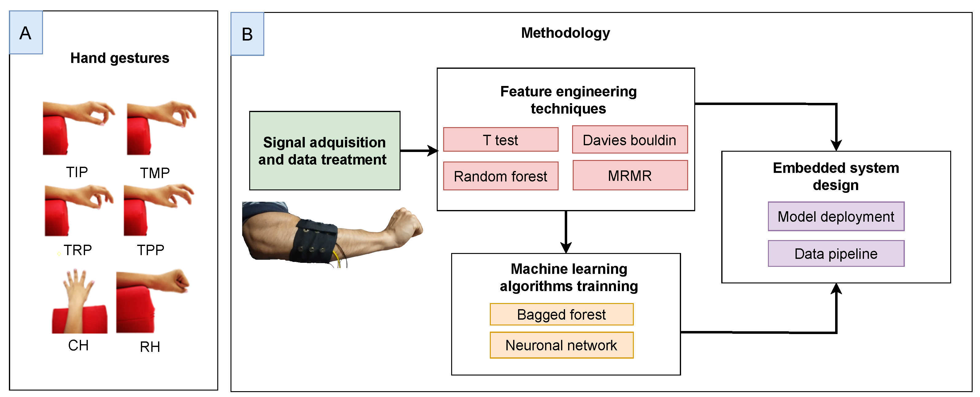Figure 1 shows the main stages involved in this study. Also, we present the deployment of complex ML models running directly from an embedded system (ESP32S3 chip), requiring specific model tuning to optimize computational performance.

2.1. Data Acquisition

Figure 2 presents the general architecture proposed for this project. The hand gestures defined in this work consist of thumb index pinch (TIP), thumb middle pinch (TMP), thumb ring pinch (TRP), thumb pinky pinch (TPP), closed fist/closed hand (CH), and neutral hand/rest hand (RH). The initial dataset consists of data from twenty healthy subjects with normal mobility of the upper extremities. The signals are sampled at 500 Hz using a band of electrodes that use the BioAmp EXG Pill as a bio-potential signal acquisition board. The band has eight electrode channels that measure forearm muscle activation signals captured by surface electromyography, where each channel is equipped with a 3-electrode configuration, comprising 2 differential electrodes and a reference electrode. The data collection sessions are synchronized through the use of videos that serve as a reference for the volunteers. This method enables the establishment of specific temporal markers for all subjects, thereby facilitating the gesture detection process.

We propose the evaluation of different feature engineering techniques (t-test, Davies–Bouldin index, random forest, and minimum redundancy maximum relevance—MRMR) to improve the performance (accuracy and complexity) of the corresponding machine learning algorithms that are trained to recognize hand gestures (bagged forest and neural networks). These stages are paramount in order to achieve our ultimate goal of properly deploying these techniques in constrained embedded systems.

2.2. Data Treatment

The raw signals are then filtered using a bandpass filter (20 to 249 Hz) and a notch filter at 60 Hz. Following the process of feature extraction, the complete dataset is segmented and labeled into 200 ms windows, with a $80\%$ overlap between samples. After reviewing the most commonly used features in the state of the art, 18 of them were selected, with each feature being calculated for each of the 8 available channels. The selected features are listed in

Table 1. Commonly used features related to EMG signals. Adapted from [18].

Index	Descriptor	Description	$\mathcal{O}\left(\right)$
1	RMS	Root Mean Square: measures the magnitude of a signal.	$\mathcal{O}\left(n\right)$
2	STD	Standard Deviation: measures the dispersion of data relative to the mean.	$\mathcal{O}\left(n\right)$
3	Var	Variance: measures the variability of data relative to the mean.	$\mathcal{O}\left(n\right)$
4	MAV	Mean Absolute Value: average of the absolute values of the signal.	$\mathcal{O}\left(n\right)$
5	WL	Waveform length: sum of the absolute differences between successive points of the signal.	$\mathcal{O}\left(n\right)$
6	Mean	Arithmetic mean: sum of all values divided by the number of values.	$\mathcal{O}\left(n\right)$
7	ZC	Zero Crossings: number of times the signal crosses the zero axis.	$\mathcal{O}\left(n\right)$
8	Kts	Kurtosis: measures the proportion of outliers in the data distribution.	$\mathcal{O}\left(n\right)$
9	Skw	Skewness: measures the asymmetry of the data distribution.	$\mathcal{O}\left(n\right)$
10	iEMG	Integrated EMG: accumulative sum of the EMG signal.	$\mathcal{O}\left(n\right)$
11	SSC	Slope Sign Changes: number of changes in the direction of the signal.	$\mathcal{O}\left(n\right)$
12	WAMP	Williston Amplitude: amplitude of the signal.	$\mathcal{O}\left(n\right)$
13	PF	Peak Frequency: frequency of the maximum amplitude of the signal spectrum.	$\mathcal{O}\left(n^3\right)$
14	PM	Peak Magnitude: maximum amplitude of the signal spectrum.	$\mathcal{O}\left(n^3\right)$
15	MNF	Mean Frequency: average frequency of the signal’s spectral distribution.	$\mathcal{O}\left(n^3\right)$
16	MNM	Mean Magnitude: average magnitude of the signal’s spectral distribution.	$\mathcal{O}\left(n^3\right)$
17	MDF	Median Frequency: frequency that divides the signal power spectrum into equal-amplitude regions.	$\mathcal{O}\left(n^3\right)$
18	MDM	Median Magnitude: median magnitude of the signal’s spectral distribution.	$\mathcal{O}\left(n^3\right)$

, and the order within this list is the same that will be used throughout the document to facilitate visibility within the graphs.

In Table 1, we make an important effort on creating a classification of the features’ complexity utilizing the Big $\mathcal{O}$ notation. This complexity is particularly important in the TinyML context as this computational power needs to be considered in addition to the main execution of the ML classification model. Here lies the importance of what we define as tiny feature engineering.

2.3. Feature Ranking

In order to evaluate these selected features, we used 4 different methods, which are described as follows:

• Random forest is chosen for being the classical example of an explainable model and for its simplicity. Random forest calculates the importance of each feature based on the average capacity of decision trees to reduce the impurity of a dataset using a specific feature. The implementation of the algorithm is composed of 100 estimators.
• The MRMR (minimum redundancy maximum relevance) method is evaluated based on the intuitive concept behind its functioning and its popularity in machine learning applications. The best features are those with the greatest importance and minimum redundancy relative to other features. The F-test and the Pearson correlation are used as relevance and redundancy metrics, respectively.
• The t-test is a very popular statistical test that assesses whether two datasets have a significant difference between their means. The null hypothesis is defined as the means of the two classes being equal, and the p-value is used to measure the degree to which the means are significantly different. The t-test is performed on all pairs of features, and the final result obtained for each feature is the mean of the p-values.
• Davies–Bouldin index. This metric is the ratio of intraclass and interclass distances in the decision space of the problem. The best features will be those that minimize this ratio, meaning that it is necessary to maximize the distances between classes and minimize the distances between samples of the same class in the decision space.

2.4. Feature Evaluation

Each of the eight channels of each sample is analyzed separately. From this point on in the paper, the 18 selected features are referred to as global features, and the 144 values calculated as the feature per channel are known as channel-specific features.

Each feature evaluation technique is compared against the classification results of two ML algorithms:

• Bagged forest (BF): The focus of this algorithm is on a small implementation of 100 estimators.
• Neuronal networks (NN): Far from a large deep learning model, in this paper, a very simple topology of a one-hidden-layer neuronal network architecture is proposed. The NN is composed of 144 neurons activated with a ReLU function.

To facilitate analysis and understanding of the results of the model, each algorithm was trained with 144 subsets of the total channel-specific features. Each subset k is composed of the k best channel-specific features. Therefore, the first subset consists of the single best channel-specific feature, the second subset consists of the two best channel-specific features, and so on until the 144th subset, which includes all channel-specific features of the dataset.

As an approximation of the importance of each channel-specific feature, the sum of the scores of the four proposed techniques is used. For this reason, all of the results are scaled between zero and one and adjusted to serve as maximization metrics. Based on the results obtained by the models, it is possible to understand the real impact of a channel-specific feature as the increment in the accuracy on the test-set with respect to the previous subset training.

2.5. Model Deployment

The training and deployment of models is contingent upon the results obtained from feature engineering. The deployment processes of neural networks and bagged forests are drastically different. On the one hand, the deployment process of neural networks involves the exportation of these networks using the edge impulse framework infrastructure, noting that no transformation process, such as pruning or quantization, is performed during this stage. On the other hand, the bagged forest undergoes a pruning process that involves the manipulation of the cost complexity parameter ccp-alpha to 0.001. Furthermore, each estimator is converted sequentially to the C programming language by transforming its thresholds and bifurcations into if-else statements. This process is facilitated by the Python library Everywhereml (v0.2.40).

The predictive accuracy of the AI model implemented on hardware was estimated using a sampling methodology based on proportions on the test set, targeting a 95% confidence level and a 3% margin of error. A conservative value of p = 0.5 was assumed to maximize variance and ensure a cautious sample size estimation, with key parameters including a Z-score of 1.96 and an error margin of 0.03. Given the finite nature of the test set, which contained 17,520 samples, a finite population correction was applied, resulting in an adjusted sample size of approximately 1008 observations. The sample is selected in a manner that ensures equilibrium in the number of observations across the six classification classes. This methodological approach enables an efficient and statistically robust evaluation of the model’s performance on the embedded system relative to its performance on a standard computer.

2.6. Embedded System Design

The architecture presented here consists of a processing pipeline structured in interconnected blocks, beginning with the acquisition of raw surface electromyographic (sEMG) signals and culminating in the system’s output, which displays the recognized gesture. Each constituent element within the pipeline functions autonomously and is assigned a specific role, thereby promoting modularity, code reusability, and ease of maintenance.

As illustrated in Figure 3, the architecture of the designed embedded system can be observed in its entirety. The eight interconnected modules collectively transform raw biosignals into meaningful classifications, thereby enabling real-time gesture recognition. The choice of hardware for the deployment of the model is the XIAO Seeed Studio ESP32S3 module (manufactured in China). This board features a small footprint (21 mm × 17.8 mm) and a 32-bit Xtensa LX7 240 MHz dual-core processor.

The software operates on an interrupt-assisted pooling cycle, with a base interrupt operating at 500 Hz and controlling the execution of the Timer block as well as the analog reading of the input signals to prevent data loss. Upon execution of the interrupt routine, the EMG Sampling block is responsible for storing a sample for each of the n channels of the system in the Circular Buffer. Concurrently, the Timer block is tasked with updating the time vectors that govern the execution of the Segmentation and Display blocks.

The Segmentation block is responsible for creating 200 ms signal windows for subsequent model prediction. In the present implementation, there is no overlap, and thus, by default, the last 100 data points available in the Circular Buffer are taken. Prior to the data’s delivery to the model, a notch filter and a bandpass filter are employed to apply a filtration process, and the corresponding features are extracted.

Subsequent to the execution of the prediction vector by the model, this result is stored in the Display block, which, in turn, stores the prediction state of the overall system. It is important to note that this final block does not constitute a physical display. Rather, its purpose is to facilitate post-processing, with the objective of generating a coherent response for the user.

3. Results

The results of each of the four techniques proposed are presented in Figure 4. These images allow for analyzing the performance of the 144 channel-specific features mapped between the 8 channels and the 18 global features proposed. The results obtained from these experiments are generally consistent with one another. The most significant variable appears to be the source channel, with the exception of the features Mean, Kts, and iEMG. All of the features exhibit a certain degree of predictive capability, and channels 3 and 4 appear to contain more valuable information.

Comparing the results of Figure 4, it is easy to notice that the t-test varies drastically from the results of the other methods. This technique appears to be very optimistic, as most of the channel-specific features are measured closer to one (many yellow blocks). Figure 5 shows the box plot of the results of the four proposed techniques.

The classification accuracy for each of the proposed models is presented in Figure 6. As each new channel-specific feature is added to each subset, it is possible to understand the contribution to the classification capacity of the ML model, as the accuracy of the model increases. At first sight, the results are consistent with the estimation based on the four proposed techniques, as the first channel-specific features enhance the model classification capacity to a greater extent than the later channel-specific features. The results seem to be very similar between them; in fact, all the algorithms reach peak performance around the 80 subset. From there, each new channel-specific feature does not significantly increase the accuracy.

Based on these results achieved by each of the ML models (presented in

Table 2. Accuracy contribution for the top 10 most relevant feature indexes for each ML model.

Index	Feature	Channel	BF	NN
54	RMS	4	$25.5\%$	$6.3\%$
93	MAV	6	$9.2\%$	$3.8\%$
68	MNF	4	$7.7\%$	$10.7\%$
51	MNM	3	$6.4\%$	$2.7\%$
42	ZC	3	$4.9\%$	$2.3\%$
17	MDM	1	$3.3\%$	$1.7\%$
94	WL	5	$1.4\%$	$1.3\%$
57	MAV	4	$3.2\%$	$0.0\%$
119	WAMP	7	$2.4\%$	$1.2\%$
50	MNF	3	$1.7\%$	$1.0\%$
64	SSC	4	$1.5\%$	$1.1\%$

), we can observe the contribution of the 10 most relevant channel-specific features of each model. Notice that these features have a higher contribution in total and remain close to $65\%$ of the total accuracy reached by the bagged forest and $30\%$ obtained by the neuronal network. It is crucial to consider that the features of the two models are essentially analogous, with the exception of two channel-specific features. The first of these, feature 94, is positioned at the seventh position in the neural network, while in the bagged forest, it is positioned at the twelfth position. The second channel-specific feature, feature 57, exhibits virtually no predictive capability in the neuronal network. Taking a closer look at Table 2, we can observe that the accuracy results are very similar between each ML model, making them extremely comparable. The global features that have the highest occurrence are MNF and MAV while the superiority of channels 3 and 4 is consistent with the findings obtained through feature engineering methods.

Figure 7 shows a brief summary of the results from our experiments. Figure 7a,b permit visualization of the score computed from the sum of the results obtained from the four feature engineering methods selected after scaling between zero and one. Figure 7a illustrates the score of the top 80 features, which, as indicated by the results in Figure 6, preserve the entire predictive capability attained. Conversely, Figure 7b depicts the score of the top 64 features, where some predictive ability is compromised, yet channels 2 and 8 may be excluded from the processing. It is essential to clarify that, in both scenarios, the Mean, Kts, and iEMG features can be removed without any issues.

The representation in Figure 7 makes it possible to compare the feature ranking as a whole, with respect to the estimation from the two ML models. The calculations of the four methods do not seem to highlight all of the channel-specific features of Table 2. At the same time, many of the channel-specific features that the feature engineering methods selected as more relevant fail to achieve that relevance in the models’ results. This suggests that even if feature engineering methods are incapable of exactly identifying the most important features, they are able to identify them as promising features from all the specific channel features.

The impact of the reduction in dimensionality, as a consequence of feature selection (fewer inputs for the ML model), can be found in

Table 3. A comparison of the trained models was conducted using the 144-features (baseline) dataset, the 80-best-features dataset, and the 64-best-features dataset.

Implementation	Models	Clock Cycles	Time [s]	Memory [KB]
Baseline	BF	$5.14\times {10}^5$	$2.14\times {10}^{-3}$	530
80 Best features per channel	BF	$5.38\times {10}^5$	$2.24\times {10}^{-3}$	523
64 Best features per channel	BF	$5.21\times {10}^5$	$2.17\times {10}^{-3}$	512
Baseline	NN	$1.26\times {10}^6$	$5.24\times {10}^{-3}$	466
80 Best features per channel	NN	$1.12\times {10}^6$	$4.66\times {10}^{-3}$	449
64 Best features per channel	NN	$9.6\times {10}^5$	$4.0\times {10}^{-3}$	432

. Each model was trained with three different datasets: one containing all 144 features (baseline), a second containing the best 80 features, and a third with the best 64 features. The recorded measurements of clock cycles and time represent the average duration required for the model to predict a single sample on the embedded system. As evidenced, by using lower features, all algorithms demonstrate a significant reduction in memory size; moreover, a substantial decrease in average inference time is observed for the neuronal networks, whereas the bagged forests exhibit stability in this regard.

An analysis of the results of the predictions of the models in

Table 4. A comparison of the predictive capabilities of models in test and validation sets on the PC, as well as models in embedded systems.

Implementation	Model	Validation Set	Test Set	Embedded Predictions
Baseline	BF	$76.35\%$	$76.10\%$	$76.0\%$
80 Best features per channel	BF	$76.24\%$	$76.06\%$	$76.0\%$
64 Best features per channel	BF	$76.24\%$	$76.06\%$	$75.0\%$
Baseline	NN	$91.38\%$	$91.41\%$	$89.72\%$
80 Best features per channel	NN	$93.67\%$	$93.65\%$	$94.21\%$
64 Best features per channel	NN	$92.23\%$	$92.19\%$	$91.82\%$

reveals a substantial discrepancy between the neural networks and the bagged forest, given that the pruning of the trees using the ccp-alpha parameter is rather aggressive. The outcomes of the bagged forest are consistent with the anticipated results, indicating that the baseline and the 80 most salient features exhibit comparable performance, and the implementation with the 64 best features exhibits a modest decline in performance. Notably, the implementation of neural networks that demonstrated superior performance was the one trained with the 80 most salient features, while the baseline exhibited the least favorable outcome.

With regard to the execution times of the embedded system, the bottleneck is identified as the calculation of the features on the segmented windows.

Table 5. A comparison of the baseline and optimized implementations in terms of the time required for the execution of the embedded feature calculation.

Implementation	Channels	Features	Clock Cycles	Time (s)
Baseline	8	18	$2.31\times {10}^6$	$9.64\times {10}^{-3}$
80 Best features per channel	8	15	$1.95\times {10}^6$	$8.12\times {10}^{-3}$
64 Best features per channel	6	15	$1.48\times {10}^6$	$6.16\times {10}^{-3}$

illustrates the impact of the dimensional space of the features on the execution times of the feature extraction. Consequently, reducing the dimensional size has the potential to enhance not only the performance of the model but also the efficacy of the pre-processing pipeline.

Table 6. The percentage reduction of implementations resulting from the application of feature engineering techniques with respect to the baseline.

Implementation	Model	Time Optimization
80 Best features per channel	BF	$12.1\%$
64 Best features per channel	BF	$29.3\%$
80 Best features per channel	NN	$14.1\%$
64 Best features per channel	NN	$31.7\%$

presents the proportion of overall optimization attained, considering both the duration of feature extraction and model prediction processes.

4. Discussion

The proposed methodology for assessing the true importance of features relies on the increase in accuracy of a specific model trained on two distinct datasets that differ by only a single feature. While this computation is straightforward and intuitive, it is crucial to acknowledge several implications. For instance, the first specific-channel feature serves as the initial reference baseline and is not necessarily the most important feature, as it lacks a comparative reference. Furthermore, it is challenging to isolate the contribution of an individual feature from the potential synergistic effects of all specific-channel features within a subset.

The management of resources constitutes a critical aspect of tinyML applications, particularly in problems such as hand gesture identification. In such cases, it is necessary to create data processing pipelines that can handle high-dimensional feature spaces. The employment of feature engineering techniques, such as feature ranking and selection, confers a heightened degree of control over the final performance of the system. The proposal illustrates how the strategic application of intelligent data management can yield performance enhancements ranging from 12% to 31%.

A survey of the literature on motion identification in resource-constrained devices reveals a paucity of interest in the application of feature engineering techniques to optimize system performance [8,9,10,11,12]. Proposal [10] does not address the influence of dimensionality reduction within the feature space. Instead, it concentrates on the reduction of complete channels to examine the effect on the overall accuracy of the model while not considering the implications for the system as a whole.

While the majority of the works utilized eight channels for the acquisition of signals [8,9,10,11], Ref. [12] employed merely four channels; these calculate a reduced number of features, at least in comparison to the present work. It is also notable that no proposal calculates features in the frequency domain, which suggests that the time required to calculate the features is less than that of the present work.

Each proposal employs distinct strategies to enhance the performance of its devices, such as accelerating response times, optimizing memory usage, or enhancing model accuracy. Specifically, the studies referenced in [9,10,11] implement hardware-based strategies to boost performance. In contrast, other works, including [12], refine the acquisition pipeline by utilizing automatic gesture detection algorithms, ensuring features are extracted only when necessary. The research presented in [8] introduced novel models aimed at reducing inference times and improving accuracy, while [11] strove to minimize the model’s in-memory demands through quantization techniques.

Table 7. A comprehensive overview of the key features inherent to advanced low-resource embedded systems for motion intent classification.

Project	Model	Inference Time	Memory	Consumption	Accuracy
[8]	LDA	$7.5\times {10}^{-2}$ s	unknown	$2.66\times {10}^{-2}$ W	0.91
[9]	SVM	$5.6\times {10}^{-4}$ s	unknown	$9.43\times {10}^{-3}$ W	0.88
[10]	SVM	unknown	9.38 KB	$2.97\times {10}^{-2}$ W	0.92
[11]	TCN	$1.28\times {10}^{-2}$ s	460 KB	$9\times {10}^{-4}$ J	0.94
[12]	NN	<$2\times {10}^{-4}$ s	unknown	$1\times {10}^{-1}$ W	0.94
This work	BF	$2.24\times {10}^{-3}$ s	523 KB	$3\times {10}^{-2}$ W	0.76
This work	NN	$4.66\times {10}^{-3}$ s	449 KB	$3\times {10}^{-2}$ W	0.94

facilitates a comparative analysis of the results obtained by the model employed in the implementation of the 80 most salient channel-specific features from this study, in relation to the current state of the art in the development of tinyML models for the identification of movement intention. A comparison of the model presented in this paper with other proposals reveals that it is comparable in terms of the metrics considered. A notable aspect is the accuracy achieved by the bagged forest, which is significantly lower than that of the other models. This suggests a potential opportunity for enhancement through the identification of less aggressive deployment methods for such models.

It is imperative to elucidate that various factors can influence the inference times of models. In this study, notable performance enhancements are realized by the elimination of features or entire channels because it addresses a high-dimensionality problem that also requires computing the FFT of each channel to compute the features in the frequency domain. Other applications that utilize a reduced number of features or require less computational effort are likely to experience more modest performance enhancements.

5. Conclusions

In this work, we compared different features associated with sEMG and selected the ones that carry most of the information in order to reduce the input dimensionality to different ML models. Such an improvement in the system is paramount in the context of TinyML applications, since we are considering deploying these solutions to heavily constrained embedded devices. Experimental results revealed that the source channel holds greater importance to this outcome. This conclusion is supported by the observation that the majority of global features demonstrate robust performance in channels 3 and 4. However, it is noteworthy that certain global features, such as the Mean, Kts, and iEMG, exhibit a conspicuously limited predictive capacity across all channels.

The global features exhibiting the highest predictive capacity are MNF and MAV. Nevertheless, among the top 10 most significant features are 6 time domain features and 3 frequency domain features. A lack of statistically significant disparities in the predictive capability of these two groups is observed; however, time-domain features possess a computational complexity of $\mathcal{O}\left(n\right)$, and the aggregate features associated with frequency manifest cubic complexity $\mathcal{O}\left(n^3\right)$.

In conclusion, portable applications for motion intention identification exhibit considerable potential for future advancements due to their distinctive characteristics. Although feature engineering techniques may encounter challenges in pinpointing the most pertinent attributes for the classification process, they remain an indispensable component of model development. This study observed substantial improvements in the performance of both the ML model and the data pipeline that supports it through the application of feature engineering strategies, thereby highlighting the critical role of these techniques in augmenting model accuracy and efficacy.