Article

An Adaptative Wavelet Time–Frequency Transform with Mamba Network for OFDM Automatic Modulation Classification

School of Space Information, Space Engineering University, Beijing 101416, China
*
Author to whom correspondence should be addressed.
AI 2025, 6(12), 323; https://doi.org/10.3390/ai6120323 (registering DOI)
Submission received: 27 October 2025 / Revised: 19 November 2025 / Accepted: 24 November 2025 / Published: 9 December 2025
(This article belongs to the Topic AI-Driven Wireless Channel Modeling and Signal Processing)

Abstract

Background: With the development of wireless communication technologies, the rapid advancement of 5G and 6G communication systems has spawned an urgent demand for low latency and high data rates. Orthogonal Frequency Division Multiplexing (OFDM) communication using high-order digital modulation has become a key technology due to its characteristics, such as high reliability, high data rate, and low latency, and has been widely applied in various fields. As a component of cognitive radios, automatic modulation classification (AMC) plays an important role in remote sensing and electromagnetic spectrum sensing. However, under current complex channel conditions, there are issues such as low signal-to-noise ratio (SNR), Doppler frequency shift, and multipath propagation. Methods: Coupled with the inherent problem of indistinct characteristics in high-order modulation, these currently make it difficult for AMC to focus on OFDM and high-order digital modulation. Existing methods are mainly based on a single model-driven approach or data-driven approach. The Adaptive Wavelet Mamba Network (AWMN) proposed in this paper attempts to combine model-driven adaptive wavelet transform feature extraction with the Mamba deep learning architecture. A module based on the lifting wavelet scheme effectively captures discriminative time–frequency features using learnable operations. Meanwhile, a Mamba network constructed based on the State Space Model (SSM) can capture long-term temporal dependencies. This network realizes a combination of model-driven and data-driven methods. Results: Tests conducted on public datasets and a custom-built real-time received OFDM dataset show that the proposed AWMN achieves a performance reaching higher accuracies of 62.39%, 64.50%, and 74.95% on the public Rml2016(a) and Rml2016(b) datasets and our formulated EVAS dataset, while maintaining a compact parameter size of 0.44 M. Conclusions: These results highlight its potential for improving the automatic modulation classification of high-order OFDM modulation in 5G/6G systems.

1. Introduction

With the advancement of wireless communication, the range and complexity of modulation techniques have significantly increased [1,2]. Additionally, growing demand from users and an exponential increase in data volume have resulted in a more complex and challenging communication environment. Novel 5G and 6G communication systems with OFDM technology have appeared with high speed and low latency [3], leading to the internet of things showing great potential in various fields. Meanwhile, in wireless communication, AMC plays a significant role in cognitive radios (CRs) and spectrum monitoring [3] and contributes to military and civilian applications, such as electronic warfare [4], radio frequency device certification [5], and unmanned vehicles [6]. With its efficient signal modulation type identification and processing capabilities, it plays an important role in communication systems requiring high efficiency and low latency, ranging from spectrum cognition in cooperative scenarios for assisting radio frequency fingerprint recognition [5] to spectrum management in non-cooperative scenarios and the identification of non-cooperative targets [3].
Existing AMC methods can be generally divided into two types: model-driven methods and data-driven methods. Model-driven methods can be divided into the likelihood-based (LB)-type AMC algorithm and the feature-based (FB)-type AMC algorithm. LB-type AMC usually focuses on mathematics-based Bayesian estimation methods, formulating the AMC task as an LB hypothesis testing problem [7,8]. Compared with the LB method, the model-driven FB method is mainly based on traditional signal processing algorithms and adopts a white-box model. It is implemented through the statistical characteristics of higher-order statistics (such as high-order moments [9] and high-order cumulants [10]) of communication signals. The two model-driven methods mentioned above have a high degree of interpretability, but both have problems. The former LB type has a sufficient mathematical derivation process, but its computational complexity is high, while the latter FB type widely uses processing transformations to effectively extract signal features, enabling its application in a wide range of industrial fields. However, it relies too much on prior expert knowledge.
With the development of big data and AI, data-driven AMC has gradually become the mainstream nowadays. The early classic methods include techniques such as support vector machines (SVMs) and decision trees [11,12]. However, the above-mentioned early data-driven methods have high requirements for data validity, which makes them ineffective at dealing with common problems in wireless channel environments such as low signal-to-noise ratios, the Doppler effect, and the multipath effect [13].
In 2018, authors proposed a Convolutional Neural Network (CNN) with truncated migration processing mechanisms that optimized the differentiation of easily confused modulation signals through multi-task learning [14], which has been proved to enjoy higher accuracy and processing efficiency than traditional CNNs. Different from this example, some authors proposed a CNN to achieve AMC tasks through the signal constellation diagrams [15]. However, its main approach is to reversely reconstruct the discrete amplitude-phase distribution constellation diagram of the signal from the chaotic received signal, and then perform modulation classification. The process of converting the signal into a constellation diagram will cause the loss of signal timing information. In 2020, authors proposed a MCNet, which was designed with several specific convolutional blocks [16] to concurrently learn spatiotemporal signal correlations via different asymmetric convolution kernels.
Unlike the previous researchers who relied on CNNs to extract local features, many other researchers have used time series features for feature extraction to assist neural networks in AMC. In 2022, the authors in [17] proposed performing AMC using Transformer, as the Mamba network based on the State Space Model (SSM) demonstrated better performance and smaller parameters than Transformer in long-time sequence tasks in 2023 [18]. Therefore, the authors [19] proposed the MAMC network in 2024, applying the Mamba network to the AMC task, with experiments showing that Mamba can effectively accomplish the AMC task. Also, some researchers [20] have proposed the novel Spiking Neural Network (SNN), which realizes the extraction of time series by utilizing the ordinary differential equation.
Different from the above studies that only focus on extracting IQ amplitude and time series features within a single local time window, some scholars have combined the two to utilize local time window and time series information in the AMC task. Researchers [21] proposed an innovative three-stream multi-channel deep learning framework for feature extraction from both single and combined in-phase/quadrature (I/Q) symbols of modulated data. Also, some researchers [22] have combined CNNs and Transformer, utilizing the global sequence effectiveness of Transformer to conduct AMC.
However, although all the above studies demonstrate the excellent performance of the computer vision field in AMC, they lack elaboration on adaptability to the signal field compared with traditional signal processing. Therefore, some researchers are currently combining traditional signal processing with neural networks to enhance the interpretability of the proposed AMC neural network models at the signal level. The author [23] proposed incorporating the Fast Fourier Transform (FFT) into the neural network feature extraction to assist the AMC task, thereby ensuring the lightweight nature of the AMC network. Reference [24] proposes a 2D-FFT and data rearrangement method to extract frequency domain scale and position features from signals, which are involved in input for feature fusion operations to assist CNN in recognition. Zhang et al. [25] designed an adaptive lifting weight wavelet feature extraction based on wavelet time–frequency transform and successfully realized the AMC by combining the attention mechanism, which achieved a good balance in terms of interpretability, model scale and recognition accuracy.
The above studies all focus on single-carrier communication. However, with the development of wireless communication, multi-carrier communication represented by OFDM has gradually played an important role in today’s communication field. At the same time, as the demand for low latency and a high data rate in communication increases, high-order modulation will become an important modulation method. Therefore, AMC needs to focus more on OFDM signals and their high-order digital modulation.
Some researchers [26] proposed an AMC algorithm using a CNN with residual learning to recognize the modulation format of the received OFDM signals of four different types of digital modulation (BPSK, QPSK, 16QAM, and 64QAM). However, the OFDM signal applied to 5G and 6G communication systems obtained high efficiency and low latency with X-PSK and X-QAM, two types with high-order digital modulation. The authors of [27] combined the attention mechanism with a CNN and LSTM to form a multi-channel AMC for OFDM, achieving AMC for nine types of digital modulations with three types of high-order modulation (BPSK, QPSK, 8PSK, MSK, 16QAM, 64QAM, 128QAM, 512QAM, 1024QAM). The authors of [28] proposed an alpha-softmax loss function and presented a deep CNN model utilizing this loss function for AMC in OFDM systems with four types of simple digital modulation schemes (BPSK, QPSK, 8PSK, and 16QAM).
Based on the discussion above, we proposed a novel AMC network for the OFDM signal; the main contributions of this paper are as follows.
  • This paper designs a network that combines traditional signal processing algorithms with deep learning networks to meet the requirements of future 5G and 6G for high-efficiency and low-latency scenarios in OFDM communication systems. To this end, adaptive wavelet transform is used for time–frequency domain feature extraction of signals, which is combined with an efficient Mamba network. Additionally, Gaussian white noise is utilized under low signal-to-noise ratios to improve performance with a smaller parameter scale.
  • The algorithm proposed in this paper is based on adaptive wavelet transform and the Mamba network (AWMN). It extracts periodic frequency and time series features from the received OFDM IQ signals by means of adaptive wavelet transform and verifies them through the publicly available RML2016.10a and RML2016.10b datasets, proving that the overall model is more effective in AMC.
  • This paper conducts real-time signal simulation experiments based on the NI LabVIEW 2020 and NI USRP 2944 software-defined radio simulation platforms, generating OFDM signals containing multiple digital modulation types. By using the KSW platform for channel simulation, we construct a real-time OFDM communication signal dataset with Doppler frequency shift and multipath effect.

2. System Models

2.1. Signal Model

For a communication system, the modulation process primarily serves to shift the spectrum of the baseband signal to a high-frequency carrier. This shift enables two key outcomes: first, the information encoded in the baseband signal can be transmitted without interference, and second, the signal can better adapt to the characteristics of the channel environment. In this paper, we have selected a typical communication model to facilitate intuitive explanation—specifically, a communication system featuring a single antenna input and a single transmitter output. This model is illustrated in Figure 1.
r s t represents the noise-free transmitted modulated signal, which can be written as
r s t = r b t e j 2 π f c t ,
where r b t represents the baseband received equivalent signal. e j 2 π f c τ i t denotes the phase changes caused by multi-path propagation, while f c is the carrier frequency, transmitted through the propagation channel model.
The received signal r r t of the communication system can be written as
r r t = r s t c t + n t
where c t represents the channel impulse response. n t represents the noise in transmission progress, such as additive white Gaussian noise (AWGN). is the convolution operation. When introducing the delay spread and multipath effect of multipath channels, the modified received signal model is written as
r r t = l = 0 L 1 h l t r s t τ l + n t
where h l t is the complex gain of the l t h multi-path, and τ l is the path delay. The signal of each path written as r s t τ l is one of the paths of the original transmitted signal r s ( t ) after a delay of τ l . The complex gain written as h l t reflects the signal decay and phase shift in that path. The convolution operation l = 0 L 1 h l t r s t τ l realizes the superposition of all multipath components, which is consistent with the synthesis mechanism of multipath signals in actual wireless channels. This explanation has been added after the formula of the received signal with multipath effects in the manuscript to clarify the association between the convolution process and multipath delays.
In real scenarios, it is necessary to add the frequency offset term f d for Doppler frequency shift, which is specifically expressed as
r s t = r b t e j 2 π f c + f d t ,
where f d = v f c / c , v is the moving speed and c is the speed of light, representing the Doppler frequency shift. The baseband received signal r b t demodulated to generate two orthogonal baseband signals, with amplitude feature A t and phase feature P t , can be written as
r b t = r I t , r Q t ,
A t = r I 2 t + r Q 2 t ,
P t = arctan r I t r Q t ,
where r I t is the in-phase samples, and r Q t is the quadrature-phase samples. For most modulated signals, the common modulation types fall into two main categories: analog modulation and digital modulation. Specifically, typical analog modulation methods include Amplitude Modulation (AM), Double-Sideband Modulation (DSB), and Frequency Modulation (FM). With the continuous development of digital signal processing technology and communication systems, digital modulation has gradually become the mainstream. Common digital modulation techniques include Frequency-Shift Keying (FSK), Amplitude-Shift Keying (ASK), Phase-Shift Keying (PSK), and Quadrature Amplitude Modulation (QAM), all of which can be expressed as
s t = E s p t e j ω c t + θ 0 ,
p ASK t = n a n δ t n T s ,
p PSK t = n e j φ n δ t n T s ,
p QAM t = n a n + j b n δ t n T s ,
p FSK t = n e j ω n ω c t δ t n T s ,
where a n and b n represent the symbol sequence. δ t represents the signal pulse and T s represents the symbol period. The variables φ n and ω n represent the modulation phase and modulation frequency. ω c denotes the carrier frequency, and θ 0 represents the initial phase. E s represents the root-mean-square energy of the signal within a symbol period, which can be expressed as
E s = 1 T s 0 T s | s t | 2 d t
where T s is the symbol period. In digital modulation, Quadrature Amplitude Modulation (QAM) transmits information through two-dimensional joints encoding “amplitude and phase”. The modulation order (such as 16QAM, 64QAM, 256QAM) directly determines the complexity of the constellation diagram and the anti-interference ability of the signal. Compared with low-order modulation, the quadrature sequence has significant “distinguishing features” within one symbol period.
For low-order digital modulation, taking QPSK as an example, it uses a n and b n to take two values:
a n , b n { + 1 2 , 1 2 } ,
a n 2 + b n 2 = 1 .
Substitute the outcome into the amplitude formula as follows:
A t = s 1 2 2 + 1 2 2 = s .
Its amplitude is fixed; substituting it into the phase formula, we can obtain only four results (0°, 90°, 180°, 270°), with a constant phase interval of 90°. Its phase characteristics change significantly and can be directly captured through time-domain statistics.
For higher-order digital modulation, taking 256QAM as an example, a n and b n each have 16 discrete values, which are the quadrature branch symbol sequence coefficients of QAM, written as
a n , b n { ± 1 , ± 3 , , ± 15 } 1 16 16 2 1 3
Substituting into the IQ signal related formula, the discrete amplitude states can be obtained as follows:
A t = s a n 2 + b n 2 .
Due to the 256 possible combinations of a n and b n , A t can exhibit up to 32 discrete states; the phase interval of P t is reduced to 1.4°, which is much smaller than the 90° of QPSK. The distinguishability of phase changes drops sharply, showing intensified high-frequency fluctuations. This dense distribution of multiple states directly causes the IQ sequence to change from low-dimensional separable features to high-dimensional mixed features.
Considering the discussion above, the essence of high-order QAM is to achieve high spectral efficiency through multiple combined values of a n and b n . The number of discrete states of its IQ sequence increases as 2 n with the order, and the time-domain characteristics change from sparse separability to dense overlap. Moreover, the rate of amplitude increases linearly with the order, and high-frequency fluctuations render traditional time-domain statistics ineffective. Finally, the sensitivity of features to noise interference increases exponentially with the order, further obscuring the learnable discriminative features.

2.2. Lifting Wavelet

Lifting wavelet is a type of wavelet transform implementation paradigm proposed by Sweldens in 1998 [29]. Its core idea is to perform multi-scale decomposition and reconstruction of signals through “Lifting Steps”, without relying on the complex Fourier transform in traditional wavelet transforms. It is an important extension and optimization of the classic wavelet theory. In contrast to traditional wavelets, such as Daubechies wavelets, the key distinction of lifting wavelets lies in the locality and flexibility of their construction process. Traditional wavelet methods, based on convolution, use global wavelet basis functions to perform inner products with signals. In contrast, lifting wavelets generate “wavelet-like basis functions” through a series of localized operations, i.e., splitting, prediction, and updating, on the signal itself. This dynamic approach enables lifting wavelets to be more adaptable and efficient, particularly when handling finite-length signals.
Splitting involves splitting the signal into two non-overlapping components according to the parity of indices, namely the even-index component x even = { x 2 k } and the odd-index component x odd = { x 2 k + 1 } . The former serves as the initial approximation component, and the latter serves as the prototype of the detail component to be processed.
Prediction involves estimating the odd-index component x odd using the approximation component x even through a fixed prediction function P . The main difference between the two is the detail component reflecting the high-frequency domain changes in the signal d = x odd P x even .
Updating involves introducing a fixed update function U to correct the approximation component x even using the detail component d , resulting in a smooth approximation component that retains the global characteristics of the signal a = x even + U d .

3. Proposed Model

Generally, the proposed model realizes the extraction of frequency domain features through adaptive wavelet transform, which in turn realizes the extraction of time–frequency domain features through lifting wavelet method, and realizing AMC through the Mamba network.

3.1. Adaptive Wavelet

The proposed adaptive wavelet block integrates learnable adaptive wavelet with a CNN to achieve the adaptive time–frequency domain features of the input signal, with the input signal represented as
x seq R B × T × C
where B is the batch size, C is the number of channels, and T is the temporal length of time step. Here, we use the IQ signal and set T = 2. The time step differs depending on the dataset used. If it is RML 2016, T = 128; if it is the OFDM dataset that we proposed, T = 1024.
Signals modulated via I/Q consist of two mutually orthogonal channels. To concurrently capture the inter-relationship between the I and Q channels, it is necessary to integrate the signal with a tensor dimension of 2 , L into a tensor with a dimension of 1 , L . For this purpose, a convolutional layer with a kernel size of ( 2 × 7 ) is employed. This convolutional layer is equipped with 64 filters, which serve to enhance the diversity of the extracted features. To further obtain higher-level features, two additional convolutional layers are applied. After undergoing processing by these two layers, the tensor shape is transformed from the original N , 1,2 , L to ( N ,   64 ,   L ) .
First, the adaptive wavelet transform uses splitting, which mainly divides the input signal into even-indexed components and odd-indexed components through slicing operations:
x even = { x 0 , x 2 , , x T 2 } R N × C × T / 2
x odd = { x 1 , x 3 , , x T 1 } R N × C × T / 2
Second, the odd components are predicted using the even components through prediction to obtain high-frequency details H. The function P for prediction is mainly set as two convolutional layers and an activation function, which can be specifically written as
P z = Tan h W P 2 LeakyReLU W P 1 z + b P 1 + b P 2
where W P 1 R C × C × k 1 describes the first-layer convolution kernel (where k 1 = 3), and W P 2 R C × C × k 2 represents the second-layer convolution kernel. W P 1 and W P 2 are both learnable prediction convolution kernels, keeping the output dimension consistent with x even . b P 1 , b P 2 R C are both bias terms, representing the learnable parameters of W P 1 and W P 2 , respectively. A complete linear map is constructed by linearly shifting the convolution results. represents the 1D convolution operation, keeping the number of channels and the length unchanged. The calculation for determining the high-frequency details of H through P is written as,
H = x odd P x even R N × C × T / 2
The high-frequency details are the difference between the odd components and the values predicted by P, and they are mainly used to reflect the high-frequency fluctuations in the signal that cannot be predicted by the low-frequency trend.
Moreover, the even components are optimized using the detail components through the update function U to obtain the low-frequency approximation L . Its design is the same as that of P symmetry, and it is also written as
U z = Tan h W U 2 LeakyReLU W U 1 z + b U 1 + b U 2 ,
where W U 1 , W U 2 , b U 1 , and b U 2 , are used to update the learnable parameters of the U function. As for the low-frequency component L of the signal, its updating mechanism is also similar to that of the high-frequency component H , which is written as
L = x even + U H R N × C × T / 2
The long timing sequence of high-order QAM needs to maintain the inter-symbol timing correlation. The update step feeds back the effective timing information in high-frequency details to low-frequency components through U ( z ) . It enabled L to not only retain global timing information but also avoid the timing truncation of traditional low-pass filtering.
By combining wavelet transform with the neural network through the above splitting–prediction–updating method, the wavelet coefficients of the central convolution kernel can be adaptively determined, thus overcoming the disadvantage that traditional wavelet bases cannot be optimized through backpropagation.

3.2. Mamba Block

The Mamba module is primarily based on the SSM, utilizing first-order differential equations to represent the evolution of latent states and output sequences. It models the sequence as a dynamic system where the current state ( h t ) evolves with time, enabling the accumulation and transmission of temporal information across long sequences. Given the known conditions of the system, the input sequence ( x t R D ) can be mapped to the output ( y t R N ) and the next state ( h t + 1 t R N ) through the current state ( h t R N ). Thus, h t + 1 t can be written as
h t + 1 t = A h t + B x t ,
y t = C h t ,
where A R N × N and B , C R N × D are the system matrices to be learned. Generally speaking, the traditional Mamba model is used for AMC. Matrix A controls the “memory decay” of the state, while matrix B enables the “state injection” of input information. This linear state transition mechanism can gradually accumulate early sequence information into subsequent states, breaking the limitation of CNNs’ local receptive fields and avoiding the ( O ( L 2 ) ) complexity of Transformer self-attention.
Unlike traditional SSMs with fixed time steps, the Mamba block in this paper dynamically predicts . It is based on input features, which are used to achieve adaptive modeling of different sequence positions:
= Softplus ( W SiLU Conv 1 d x ) ,
where the input x first captures local temporal patterns through deep convolution, with a kernel size of d conv = 4 . It undergoes SiLU activation. The processed features are projected to , which matches the input dimension through the linear layer W . The W maps local features to modify , which matches the input dimension. Using the Softplus function ensures that > 0, and allows to be dynamically adjusted with the input signal for the stable segments of OFDM signals, meaning that delta increases to retain long-term information and decreases to obtain short-term details, adapting to features of different time scales.
The time step is ensured to be positive through Softplus, which is expressed as
Softplus x = ln 1 + e x .
It is particularly suitable for the long-term inter-symbol correlations of OFDM signals. To directly model the collected discrete data sequence, the aforementioned functions can be discretized, which can be expressed as
h n = A ¯ h n 1 + B ¯ x n ,
y n = C h n ,
where a time step ( ) is used for implementation, with A ¯ and B ¯ written as
A ¯ = exp A ,
B ¯ = A 1 exp A I B .
By converting the continuous form , A , B , C into the discrete form A ¯ , B ¯ , C , the model can be computed recursively in a linear manner, thus enhancing computational efficiency. To avoid the O ( L ) complexity of traditional recursive computation, the model uses a parallel scanning algorithm to perform batch processing calculations on discrete state equations as follows:
h n = PScan A ¯ , B ¯ x n ,
where the PScan operation transforms the recursive process into parallel computation through matrix decomposition, reducing the time complexity to O L l o g L . The recursive computation of the traditional discrete SSM h ( n ) has a complexity of O ( L ) . The PScan algorithm converts recursion into parallel computation through matrix decomposition. It decomposes A ¯ into multiple matrix factors that can be computed in parallel, enabling the simultaneous computation of h n at all time steps and reducing the complexity to O ( L l o g L ) , which is suitable for the efficient processing of long sequences.
This approach is implemented in the code through the following steps: precomputing A ¯ and B ¯ x n , obtaining the state h n at all time steps, and finally outputting the result, written as
h n = A ¯ h n 1 + B ¯ x n
y n = h n C T + D x n .
To satisfy the dimension matching requirement, C is transposed to C T . Also, to enhance the expressive ability of model, we introduce the matrix D     R D × D . We set a learnable parameter initialized as a zero matrix and updated through backpropagation. The model can adaptively adjust the weight of the direct input contribution based on training data. This is not a conflict with the basic SSM but an extended form of it. The rationality of this extension has been clarified in the manuscript.
Inspired by MAMC (Mamba for AMC) [19], we mainly built the Mamba classifier module based on its core ideas. Compared with the MAMC in [19], the Mamba block in this paper has removed unnecessary parts, mainly its soft thresholding denoising unit, as well as the filters, some linear projections and convolutions within it.

3.3. Loss Function

The loss function of the AWMN model in this paper adopts a multi-component joint optimization strategy, combining classification loss and regularization constraints to achieve the collaborative optimization of feature learning and classification tasks. Its mathematical expression is as follows:
L t o t a l = L C E + i = 1 L N λ d R d e t a i l s i + λ a R a p p r o x i .
L N is the number of layers in the adaptive wavelet transform. L C E is the loss of Cross-Entropy, which is used for supervised learning in direct classification tasks and is specifically expressed as
L C E = k = 1 K y k log y k ^ ,
where K is the number of classification categories, y k is the one-hot encoding of the true label, and y k ^ is the probability of each predicted category being output by the model through softmax.
R d e t a i l s i and R a p p r o x i are, respectively, the regularization terms of the detail and the approximation coefficients of the i t h level of the adaptive wavelet transform. R d e t a i l s i adopts the L2 distance constraint. By limiting the Euclidean distance between the mean value of the low-frequency components L i of the i t h layer and the mean value of the input feature xi of that layer, it maintains the consistency of low-frequency components with respect to the global trend of the signal. The expression is as follows:
R approx i = λ a × dist mean L i , mean x i , p = 2 ,
where λ a is the regularization weights (configured as 0.01), L i is the low-frequency component of the i t h layer, and x i is the input feature of the wavelet transform of the i t h layer. dist mean L i , mean x i , p = 2 represents the calculation of the Euclidean distance (L2 distance) between L i and x i two mean vectors, written as
d i s t μ L ,   μ x ,   p = 2 = i = 1 I mean L i mean x i 2 .
The constraint avoids the loss of low-frequency global information during the wavelet decomposition process and enhances the stability of the model in learning overall trends. R d e t a i l s i adopts the L 1 distance constraint, written as
R details i = λ d × m e a n H i .
λ d is regularization weights (configured as 0.01), and H i is the high-frequency component of the i t h layer wavelet transform. By taking the mean of its absolute values, the suppression of high-frequency noise and the enhancement of feature sparsity are achieved, enabling effective feature extraction.

3.4. Adaptive Wavelet Mamba Network

As with previous discussions, our adaptive wavelet transform module splits the signal into even and odd parts, which are then processed into low-frequency components and high-frequency components, respectively.
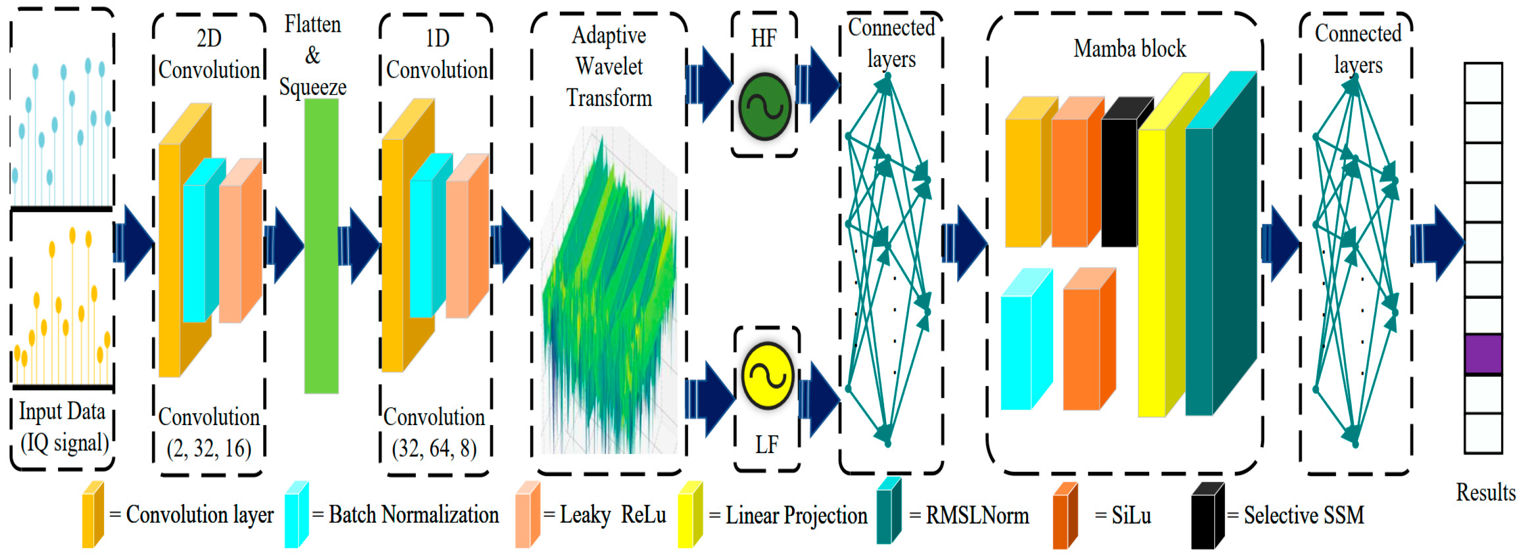
The obtained detail coefficients and approximation coefficients can efficiently extract the time–frequency features of the signal. Different from traditional discrete time series modeling methods such as LSTM and Transformer, which extract temporal features, and ResNet, which focuses on local features, it can better model and extract the features of signal sequences in the time–frequency domain. Compared with methods based on computer vision, it is more suitable for signal applications. As shown in Figure 2 and Table 1, we combine the adaptive wavelet transform with Mamba to form AWMN. Compared with Transformer, Mamba can effectively enhance the model’s ability to extract the overall features of time series through SSM, further strengthen the extraction of long-term time series features, and achieve an improvement in the overall classification accuracy rate.

4. Experiment Results and Discussion

4.1. Dataset and Experiment Settings

The experimental evaluations in this study are carried out on three datasets: RML2016.10a, RML2016.10b, and EVAS. The RML datasets are publicly available benchmarks generated through simulation using GNU Radio. In contrast, the EVAS dataset consists of real-time OFDM signals that were acquired using NI LabVIEW in conjunction with a USRP. A detailed description of these datasets is provided in this subsection.

4.1.1. RML Dataset

The model proposed in this research draws on two datasets: RML2016.10a and RML2016.10b. As noted by O’Shea [30], both datasets were created via GNU Radio. Specifically, the RML2016.10a dataset consists of IQ-modulated signals covering 11 unique modulation schemes: 8PSK, BPSK, CPFSK, GFSK, PAM4, QAM16, QAM64, QPSK, AM-SSB, AM-DSB, and WBFM. These signals feature signal-to-noise ratio (SNR) values spanning 20 intervals of 2 dB each, with the range extending from −20 dB to 18 dB. For each modulation category in this dataset, there are 220,000 communication signal samples, and every sample includes 128 sampling points. By comparison, the RML2016.10b dataset contains IQ-modulated signals corresponding to 10 modulation types—excluding AM-SSB, the list includes 8PSK, BPSK, CPFSK, GFSK, PAM4, QAM16, QAM64, QPSK, AM-DSB, and WBFM. A key difference lies in sample size: each modulation type in RML2016.10b has 1,200,000 samples, though each sample still comprises 128 sampling points, consistent with RML2016.10a.
Notably, both datasets are labeled with annotations that specify the modulation type and SNR value for individual signals. For the needs of this study, the datasets were split into training and testing subsets: 70% of the data was allocated for model training, and the remaining 30% was set aside for testing purposes.

4.1.2. EVAS Dataset Description

In contrast to the RML dataset, which is produced through GNU Radio simulations, the dataset utilized in this study comes from real-time signal transmissions and receptions—these processes are supported by the USRP RF transmitter and receiver developed by National Instruments (NI). This dataset contains IQ samples, along with matching labels that identify the respective modulation classes.
The modulation schemes taken into account in this work include BPSK, QPSK, 8PSK, 16PSK, 4PAM, 16QAM, 32QAM, 64QAM, 128QAM, 256QAM, and 512QAM. As outlined in Table 2, for each modulation type, a typical example is created for a data subcarrier with K = 256. This example covers an SNR range from −10 dB to 20 dB, using a step size of 2 dB. For each SNR value under each modulation class, there are 3000 representative examples. Additionally, the specific characteristics of the OFDM signal are further detailed in Table 2.
In our experiments, the OFDM signal data will be transmitted through the Extended Vehicular Advanced (EVA) channel, as defined by the 3GPP standard [31]. This channel model consists of nine Rayleigh fading paths, each characterized by distinct power levels and phase delays. The EVA channel is specifically designed to simulate urban scenarios with vehicular mobility, incorporating multipath effects, and is intended to reflect typical communication environments in cities that require high-speed and low-latency communication. The dataset used in this study was divided into two groups: 70% of the data was used for training and the remaining 30% for validation. The test set contains 1800 examples of each modulation class for each SNR value.
As for the public RML datasets, we split our EVAS dataset into training and testing subsets: 70% of the data was used for model training, and the remaining 30% was set aside for testing.

4.1.3. Training Configuration

This paper makes use of PyTorch 2.0.1 as the deep learning framework, with the development process carried out in the PyCharm 2023 environment. Experimental operations are supported by NVIDIA Tesla V100 GPUs, which provide the necessary computational power for model training. The model’s training relies on samples from two datasets: the RML dataset (with SNR values ranging from −20 dB to 18 dB) and the EVAS dataset (with SNR values between −10 dB and 20 dB). Because of the different scale and sampling points of the datasets, we used a total of 50 training epochs for the public Rml2016(a) and Rml2016(b) datasets and 100 training epochs for our EVAS dataset. For all datasets, a constant learning rate of 0.001 is maintained. For the optimization of the training progress, the Adam optimizer is adopted for all datasets. This optimizer integrates the strengths of AdaGrad and RMSProp, and it is selected specifically for its effectiveness in handling noisy or sparse gradient signals. Additionally, the model is trained with a batch size of 512. Notably, the model’s architecture is designed to be independent of the number of input signal samples. This design ensures consistency in performance when processing signals with a fixed length of 128 samples. To establish baseline performance and prove the advantages of our proposed model, several well-established AMC models are selected for comparison, including ResNet [14], Transformer [17], CLDNN [32], MAMC [19], MCNET [16], and AWAN [25].

4.2. Model Performance Ablation Comparison Analysis and Discussion

To precisely and comprehensively evaluate the effectiveness of the model proposed in this paper, we use the following benchmarks.
a. Maximum accuracy measures the maximum recognition accuracy of models crossing all varying SNRs;
b. Average accuracy measures the average modulation recognition accuracy between −20 dB and 18 dB for all models (−10 dB and 20 dB for EVAS dataset);
c. The number of parameters measures models’ complexity.
Firstly, as shown in Table 2, the number of parameters represents the model complexity and the computation complexity of these proposed network structures for determining the AMC accuracy of the public RML2016.10a and RML2016.10b datasets and our proposed EVAS dataset. Our proposed AWMN method had the top results for average accuracy, with 62.39%, 64.50% and 75.95%, followed closely by the AWAN model, with 61.66%, 63.48% and 74.38.
In terms of parameter scale and computational complexity, the proposed model is merely 0.44 M larger than MCNET, yet it achieves average improvements of 5.69% and 3.75%, respectively. This indicates that our proposed AWMN model not only attains the highest average accuracy across all SNR levels and the top maximum accuracy among all tested models but also exhibits lower model complexity and computational overhead compared to traditional models such as Transformer and ResNet.
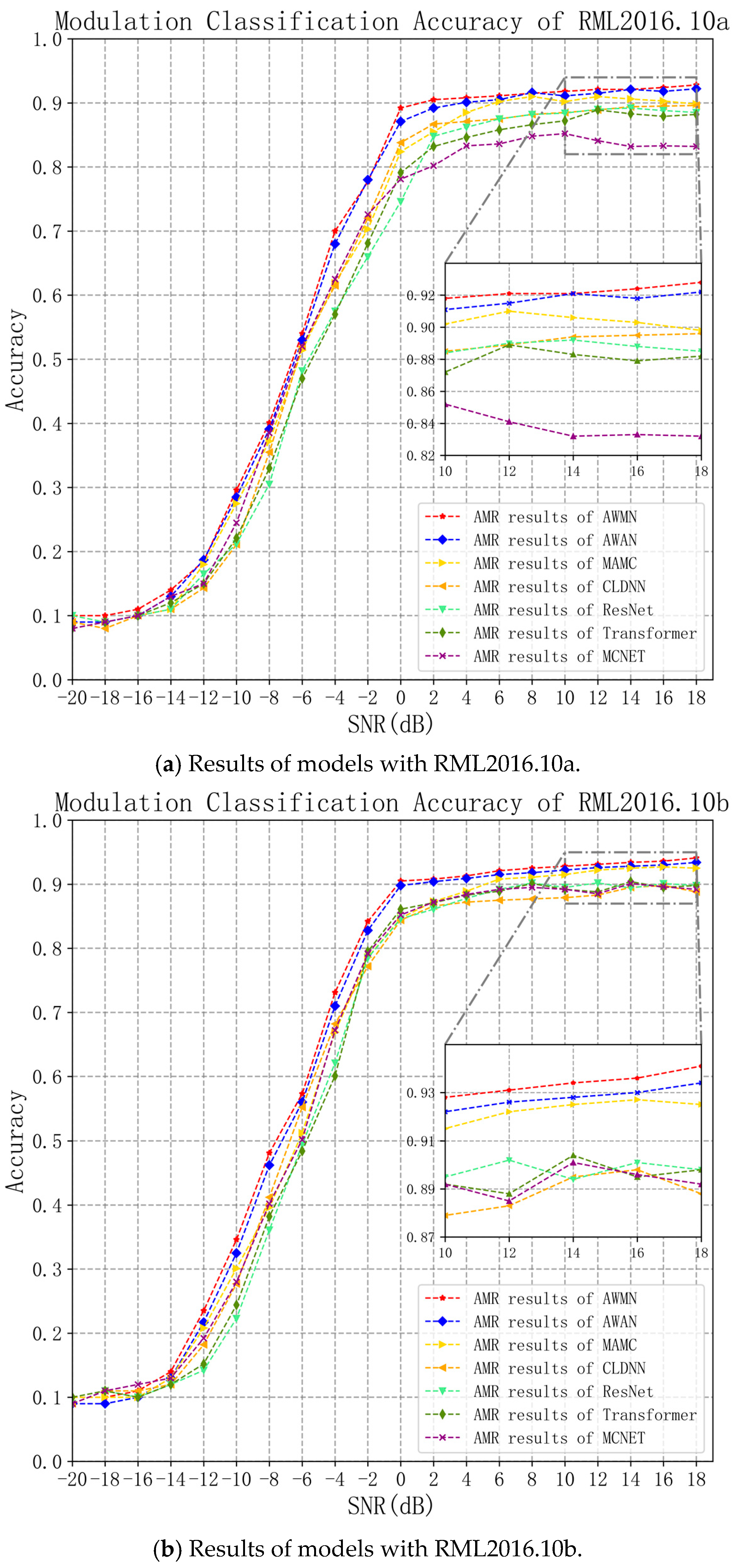
Furthermore, as the experimental results presented in Figure 3a,b demonstrate, the AMC accuracies of all models rise with the increase in the SNR, and the AWMN model outperforms others in classification accuracy. Specifically, on the RML2016.10a dataset, when the SNR reaches 18 dB, the AWMN model achieves a maximum accuracy of 92.8%, the highest among all tested models. In contrast, the AWAN model, the MAMC model, ResNet, Transformer, CLDNN, and MCNET only reach accuracies of 92.2%, 91.4%, 89.2%, 88.9%, 89.6%, and 87.1%, respectively, under the same SNR conditions.
For the RML2016.10b dataset, our AWMN obtained a maximum accuracy 94.1% as when the SNR was 18 dB, and 64.50% on average. With the AWAN model, we achieved a maximum accuracy of 93.4%, with 63.48% as the average accuracy. Moreover, MAMC, ResNet, Transformer, CLDNN and MCNET achieved maximum accuracies of 92.7%, 90.8%, 90.4%, 89.8% and 90.1%, respectively. Also, for the MAMC model, ResNet, Transformer, CLDNN and MCNET, the average accuracy only reached 61.79%, 59.52%, 59.85%, 60.42% and 60.75%, respectively.
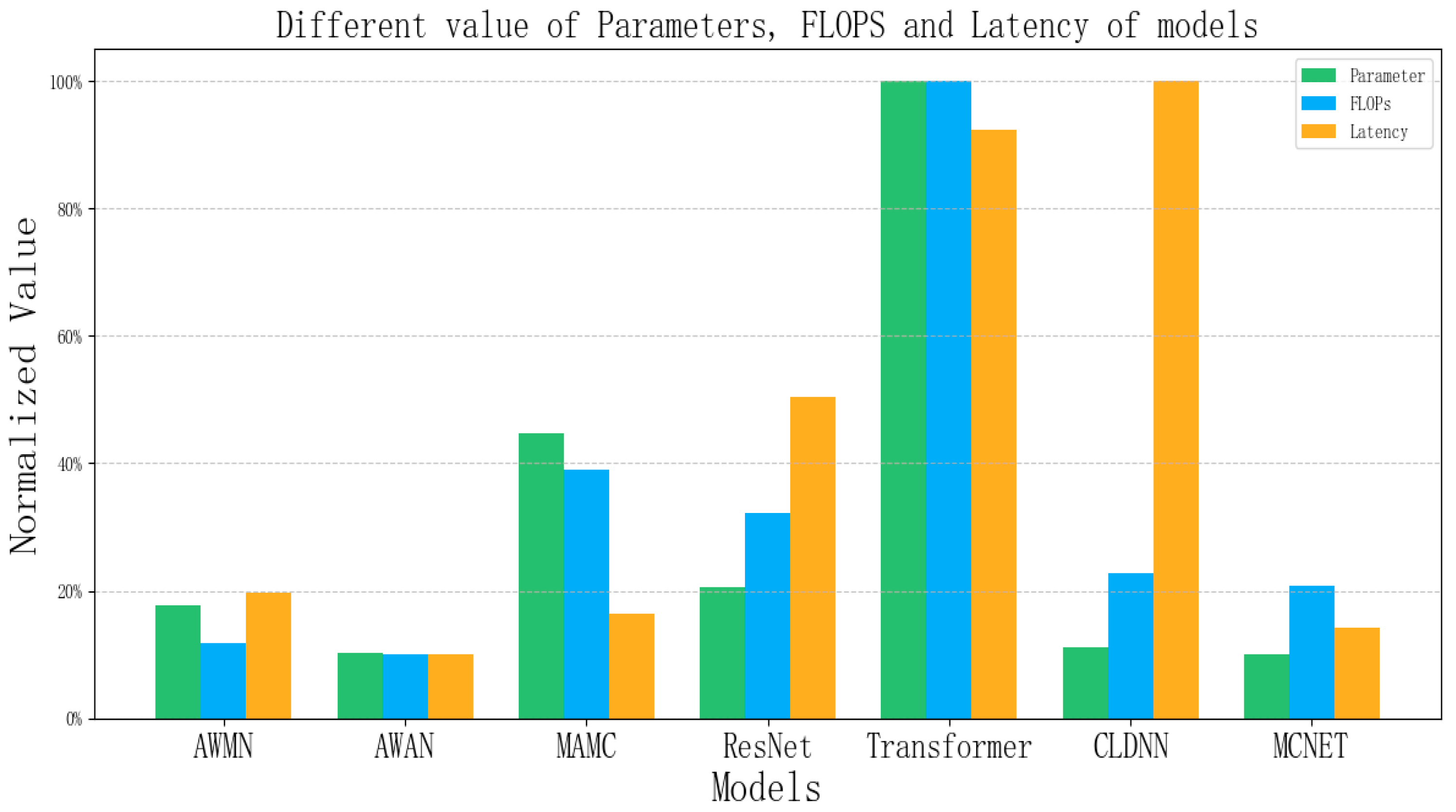
Figure 4 illustrates the perspective of network scale when training with the public RML2016(a) dataset. Due to the large differences between the different models, we took the smallest model (AWAN) as the baseline and applied normalization to highlight the distinctions among the models. Combined with the parameter shown in Table 3, the MCNET model performs the best, being 0.44 M lower than our AWMN model. As it achieves the highest classification accuracy and has relatively fewer parameters compared to all the proposed models, it balances the contradiction between the complexity and recognition accuracy of these models very well in AMC for single carrier tasks (RML2016.10a and RML2016.10b datasets).
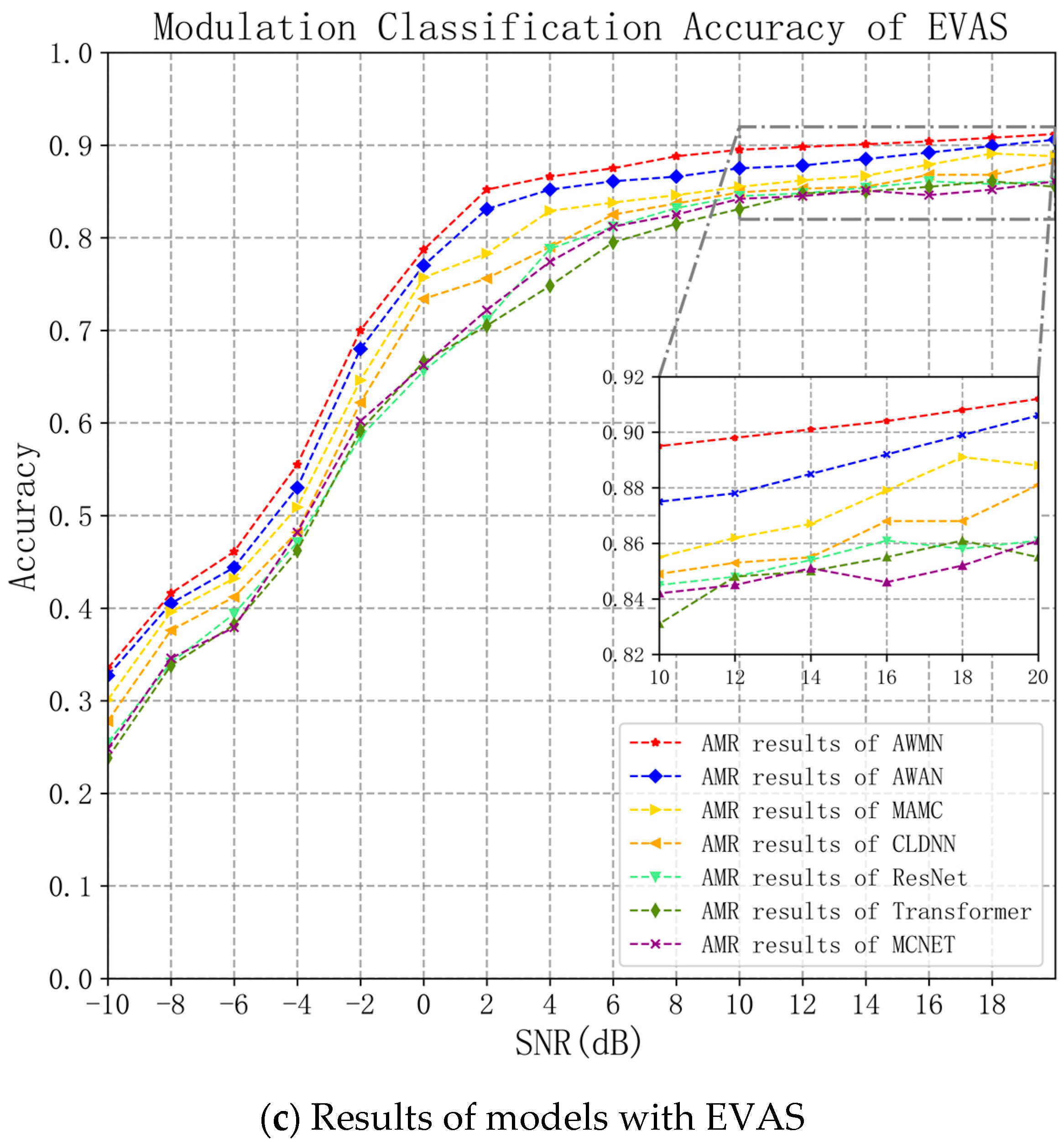
Additionally, to verify the effectiveness of our proposed AWMN model in automatic modulation classification (AMC) for OFDM and advanced digital modulation communication signals, we further conducted experiments on the self-created OFDM EVAS dataset. For this EVAS dataset, when the SNR reached 20 dB, the AWMN model achieved a maximum accuracy of 91.2%, the highest among all the models compared. In contrast, under the same SNR condition, the AWAN model, the MAMC model, ResNet, Transformer, CLDNN, and MCNET only attained accuracies of 90.6%, 88.8%, 86.1%, 85.5%, 88.1%, and 86.1%, respectively. In terms of average accuracy, our AWMN model also ranked first, with a score of 75.95%. By comparison, the average accuracies of the AWAN model, the MAMC model, ResNet, Transformer, CLDNN, and MCNET were 74.38%, 72.36%, 68.57%, 67.75%, 70.53%, and 68.43%, respectively.
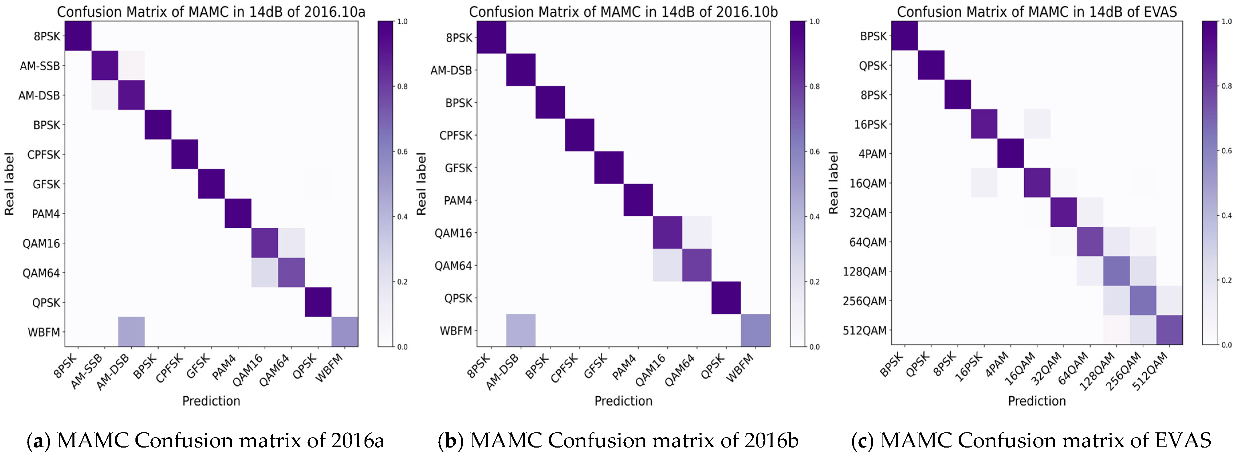
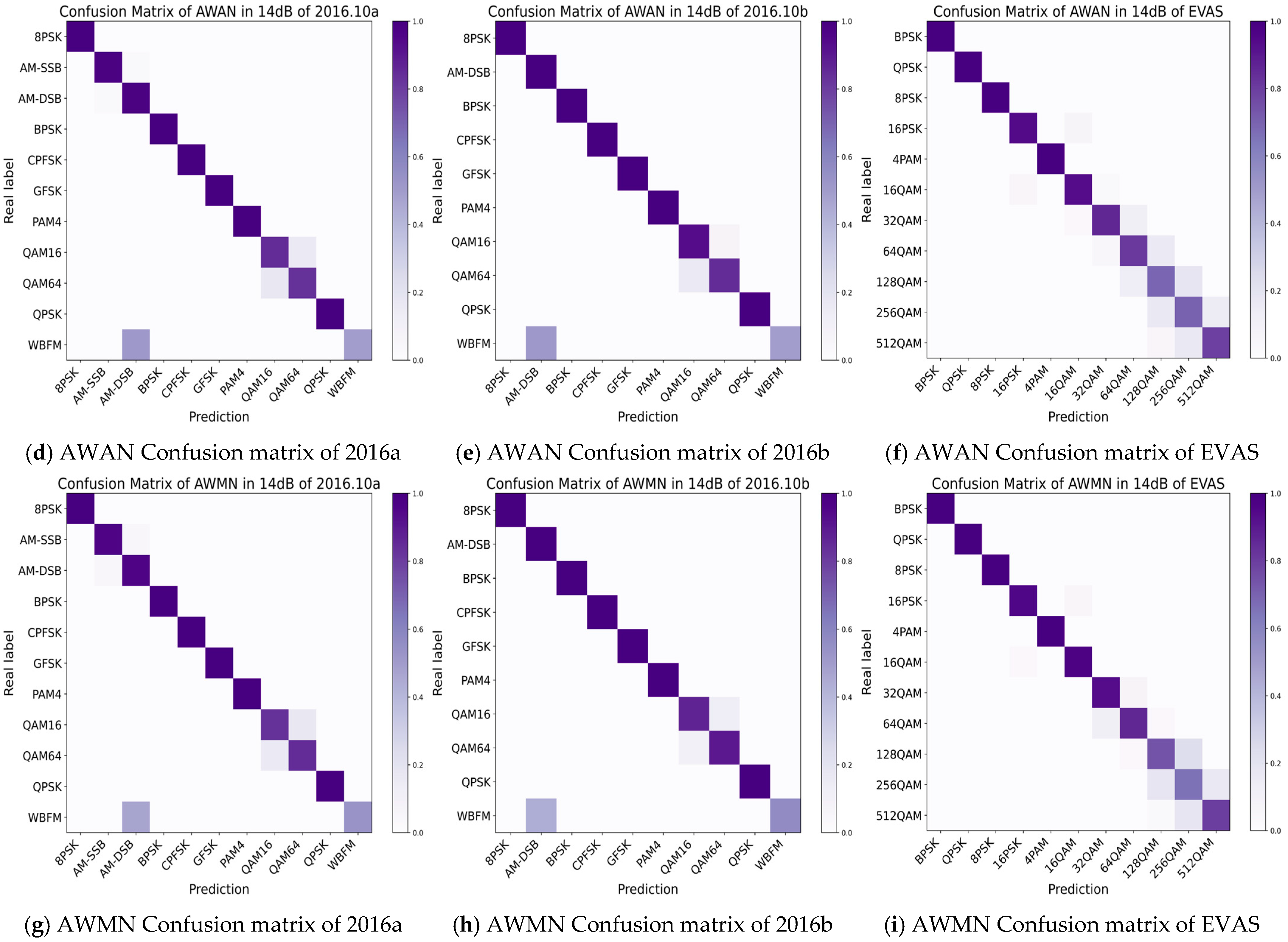
Also, as shown in Figure 5, we compare the general confusion matrices of our AWMN, AWAN, and MAMC models, which are used to show the behavior of models in model predicted classes and ground truth classes of each modulation type. As clearly shown in the results for when the SNR = 14, our model generally performed better for different types of modulation.

5. Conclusions

In this paper, we addressed the pressing demand for efficient AMC in 5G/6G OFDM communication systems, where higher-order modulation schemes and complex channel environments pose significant challenges to conventional approaches. To this end, we propose the AWMN, which integrates adaptive wavelet transforms with the Mamba architecture, and rigorously validate its effectiveness through comprehensive experiments. Firstly, the AWMN framework successfully bridges traditional signal processing with deep learning, offering a solution aligned with the efficiency and low-latency requirements of future 5G and 6G OFDM systems. The adaptive wavelet transform module, designed based on a lifting wavelet paradigm, enables trainable time–frequency feature extraction through learnable splitting, predicting, and updating operations, overcoming the limitation of conventional wavelet bases that cannot be optimized via backpropagation. When coupled with the lightweight Mamba network, this module provides robust performance under low-SNR conditions, owing to its resilience against additive white Gaussian noise, while maintaining a compact parameter size of only 0.44 M, thus striking a balance between efficiency and accuracy. Also, experimental results on three benchmark datasets demonstrate the superiority of AWMN for AMC tasks. On the RML2016.10a and RML2016.10b datasets, AWMN achieves average accuracies of 62.39% and 64.50%, with peak accuracies of 92.8% and 94.1% at a 18 dB SNR, outperforming baseline models such as AWAN, MAMC, and Transformer. On the custom-built EVAS dataset, which includes high-order OFDM modulation formats such as 512QAM, AWMN achieves an average accuracy of 75.95%, with a maximum accuracy of 91.2% at 20 dB SNR. These results highlight the strong adaptability of AWMN to high-order digital modulation and complex OFDM scenarios. The complementary strengths of the adaptive wavelet transform (capturing periodic frequency-domain features) and the Mamba network (capturing long-range temporal dependencies) enable more discriminative feature learning. Finally, our real-time simulation experiments conducted on the NI LabVIEW, NI USRP, and KSW platforms further confirm the practical utility of AWMN. By constructing an OFDM dataset incorporating Doppler shifts and multipath effects—based on the 3GPP EVA channel model for emulating vehicular urban environments—the results demonstrate that AWMN maintains high recognition accuracy under realistic communication conditions. This contribution fills a critical gap in the literature, where most prior studies have predominantly focused on single-carrier signals, and underscores the potential of AWMN for real-world OFDM spectrum monitoring and cognitive radio applications. The model and experiments proposed in this paper still have certain limitations. The experimental dataset was generated using the USRP RF device and the KSW channel simulator, but it has not been validated against real physical wireless channels. As a result, the model lacks consideration for the complexities of real-world electromagnetic environments and Doppler effects. Additionally, while this paper explores a combination of model-driven and data-driven approaches to some extent, it primarily relies on data-driven methods. There is a lack of strategies to address issues related to suboptimal samples, such as small sample sizes, sparse sampling points, and imbalanced datasets. In the future, we will focus on these aspects to enable practical applications of AI and communication.

Author Contributions

Conceptualization, H.X. and Y.L.; methodology, H.X.; software, H.X. and Y.L.; validation, H.X.; formal analysis, H.X. and Y.L.; investigation, H.X.; resources, X.T., L.W. and B.Z.; data curation, H.X., L.W. and Y.L.; writing—original draft preparation, H.X.; writing—review and editing, X.T., L.W. and B.Z.; visualization, H.X.; supervision, X.T.; project administration, X.T., L.W. and B.Z.; funding acquisition, X.T. All authors have read and agreed to the published version of the manuscript.

Funding

This work was supported by the National Natural Science Foundation of China (NSFC) under Grant 62027801.

Institutional Review Board Statement

Not applicable.

Informed Consent Statement

Not applicable.

Data Availability Statement

The public dataset is downloaded on https://gitcode.com/open-source-toolkit/dcbd5 (accessed on 27 October 2025).

Conflicts of Interest

The authors declare no conflict of interest.

References

  1. Khoshafa, M.H.; Maraqa, O.; Moualeu, J.M. RIS-Assisted Physical Layer Security in Emerging RF and Optical Wireless Communications Systems: A Comprehensive Survey. IEEE Commun. Surv. Tutor. 2025, 27, 2156–2203. [Google Scholar] [CrossRef]
  2. Doha, S.R.; Abdelhadi, A. Deep Learning in Wireless Communication Receivers: A Survey. IEEE Access 2025, 13, 113586–113605. [Google Scholar] [CrossRef]
  3. Zhang, H.; Zhou, F.; Du, H.; Wu, Q.; Yuen, C. Revolution of Wireless Signal Recognition for 6G: Recent Advances, Challenges and Future Directions. IEEE Commun. Surv. Tutor. 2025; Early Access. [Google Scholar] [CrossRef]
  4. Satapathy, J.R.; Bodade, R.M.; Ayeelyan, J. CNN based Modulation classifier and Radio Fingerprinting for Electronic Warfare Systems. In Proceedings of the 2024 4th International Conference on Advance Computing and Innovative Technologies in Engineering (ICACITE), Greater Noida, India, 14–15 May 2024; pp. 1880–1885. [Google Scholar]
  5. Ahmed, A.; Quoitin, B.; Gros, A.; Moeyaert, V. A comprehensive survey on deep learning-based lora radio frequency fingerprinting identification. Sensors 2024, 24, 4411. [Google Scholar] [CrossRef] [PubMed]
  6. Chennagiri, R.; Sehgal, S.; Ravinder, Y. A Survey on Automatic Modulation Classification Techniques. In Proceedings of the 2024 Intelligent Systems and Machine Learning Conference (ISML), Hyderabad, India, 4–5 May 2024; pp. 94–100. [Google Scholar]
  7. Xu, J.L.; Su, W.; Zhou, M. Software-Defined Radio Equipped with Rapid Modulation Recognition. IEEE Trans. Veh. Technol. 2010, 59, 1659–1667. [Google Scholar] [CrossRef]
  8. Hameed, F.; Dobre, O.A.; Popescu, D.C. On the likelihood-based approach to modulation classification. IEEE Trans. Wirel. Commun. 2021, 116, 301–310. [Google Scholar] [CrossRef]
  9. Kharbech, S.; Simon, E.P.; Belazi, A.; Xiang, W. Denoising Higher-Order Moments for Blind Digital Modulation Identification in Multiple-Antenna Systems. IEEE Wirel. Commun. Lett. 2020, 9, 765–769. [Google Scholar] [CrossRef]
  10. Huang, S.; Chen, Y.; He, J.; Chang, S.; Feng, Z. Channel-Robust Automatic Modulation Classification Using Companding Spectral Quotient Cumulants. IEEE Trans. Veh. Technol. 2024, 73, 17749–17753. [Google Scholar] [CrossRef]
  11. Li, J. Automatic modulation classification using support vector machines and error correcting output codes. In Proceedings of the 2017 IEEE 2nd Information Technology, Networking, Electronic and Automation Control Conference (ITNEC), Chengdu, China, 15–17 December 2017; pp. 60–63. [Google Scholar]
  12. Luan, S.; Gao, Y.; Chen, W.; Yu, N.; Zhang, Z. Automatic Modulation Classification: Decision Tree Based on Error Entropy and Global-Local Feature-Coupling Network Under Mixed Noise and Fading Channels. IEEE Wirel. Commun. Lett. 2022, 11, 1703–1707. [Google Scholar] [CrossRef]
  13. Dobre, O.A.; Abdi, A.; Bar-Ness, Y.; Su, W. Survey of automatic modulation classification techniques: Classical approaches and new trends. IET Commun. 2007, 1, 137–156. [Google Scholar] [CrossRef]
  14. Li, R.; Li, L.; Yang, S.; Li, S. Robust automated vhf modulation recognition based on deep convolutional neural networks. IEEE Wirel. Commun. Lett. 2018, 22, 946–949. [Google Scholar] [CrossRef]
  15. Peng, S.; Jiang, H.; Wang, H.; Alwageed, H.; Zhou, Y.; Sebdani, M.M.; Yao, Y.-D. Modulation Classification Based on Signal Constellation Diagrams and Deep Learning. IEEE Trans. Neural Netw. Learn. Syst. 2019, 30, 718–727. [Google Scholar] [CrossRef] [PubMed]
  16. Huynh-The, T.; Hua, C.-H.; Pham, Q.-V.; Kim, D.-S. Mcnet: An efficient cnn architecture for robust automatic modulation classification. IEEE Commun. Lett. 2020, 24, 811–815. [Google Scholar] [CrossRef]
  17. Cai, J.; Gan, F.; Cao, X.; Liu, W. Signal Modulation Classification Based on the Transformer Network. IEEE Trans. Cogn. Commun. Netw. 2022, 8, 1348–1357. [Google Scholar] [CrossRef]
  18. Gu, A.; Dao, T. Mamba: Linear-time sequence modeling with selective state spaces. arXiv 2023, arXiv:2312.00752. [Google Scholar] [CrossRef]
  19. Zhang, Y.; Zhou, Z.; Cao, Y.; Li, G.; Li, X. MAMC—Optimal on Accuracy and Efficiency for Automatic Modulation Classification with Extended Signal Length. IEEE Commun. Lett. 2024, 28, 2864–2868. [Google Scholar] [CrossRef]
  20. Lin, C.; Zhang, Z.; Wang, L.; Wang, Y.; Zhao, J.; Yang, Z.; Xiao, X. Fast and Lightweight Automatic Modulation Recognition using Spiking Neural Network. In Proceedings of the 2024 IEEE International Symposium on Circuits and Systems (ISCAS), Singapore, 19–22 May 2024; pp. 718–727. [Google Scholar]
  21. Xu, J.; Luo, C.; Parr, G.; Luo, Y. A spatiotemporal multi-channel learning framework for automatic modulation recognition. IEEE Wirel. Commun. Lett. 2020, 9, 1629–1632. [Google Scholar] [CrossRef]
  22. Ma, W.; Cai, Z.; Wang, C. A Transformer and Convolution-Based Learning Framework for Automatic Modulation Classification. IEEE Commun. Lett. 2024, 28, 1392–1396. [Google Scholar] [CrossRef]
  23. Zhu, Z.; Zhou, N.; Wang, Z.; Liang, J.; Wang, Z. MSGNet: A Multi-Feature Lightweight Learning Network for Automatic Modulation Recognition. IEEE Commun. Lett. 2024, 28, 2553–2557. [Google Scholar] [CrossRef]
  24. Liu, Y.; Yan, X.; Hao, X.; Yi, G.; Huang, D. Automatic Modulation Recognition of Radiation Source Signals Based on Data Rearrangement and the 2D FFT. Remote Sens. 2023, 15, 518. [Google Scholar] [CrossRef]
  25. Zhang, J.; Wang, T.; Feng, Z.; Yang, S. Toward the Automatic Modulation Classification with Adaptive Wavelet Network. IEEE Trans. Cogn. Commun. Netw. 2023, 9, 549–563. [Google Scholar] [CrossRef]
  26. Huynh-The, T.; Nguyen, T.-V.; Pham, Q.-V.; da Costa, D.B.; Kwon, G.-H.; Kim, D.-S. Efficient Convolutional Networks for Robust Automatic Modulation Classification in OFDM-Based Wireless Systems. IEEE Syst. J. 2023, 17, 964–975. [Google Scholar] [CrossRef]
  27. Kumar, A.; Chaudhari, M.S.; Majhi, S. Automatic modulation classification for ofdm systems using bi-stream and attention-based cnnlstm model. IEEE Commun. Lett. 2024, 28, 552–556. [Google Scholar] [CrossRef]
  28. Song, G.; Jang, M.; Yoon, D. Automatic Modulation Classification for OFDM Signals Based on CNN with α-Softmax Loss Function. IEEE Trans. Aerosp. Electron. Syst. 2024, 60, 7491–7497. [Google Scholar] [CrossRef]
  29. Daubechies, I.; Sweldens, W. Factoring wavelet transforms into lifting steps. In Wavelets in the Geosciences; Lecture Notes in Earth Sciences; Klees, R., Haagmans, R., Eds.; Springer: Berlin, Germany, 2000; Volume 90, pp. 131–157. [Google Scholar]
  30. O’Shea, T.J.; Corgan, J.; Clancy, T.C. Convolutional Radio Modulation Recognition Networks. In Engineering Applications of Neural Networks (EANN 2016); Communications in Computer and Information Science; Jayne, C., Iliadis, L., Eds.; Springer: Cham, Switzerland, 2016; Volume 629, pp. 213–226. [Google Scholar]
  31. Luo, C.; Tang, A.; Gao, F.; Liu, J.; Wang, X. Channel modeling framework for both communications and bistatic sensing under 3gpp standard. IEEE J. Sel. Areas Sens. 2024, 1, 166–176. [Google Scholar] [CrossRef]
  32. Tu, A.; Lin, Y.; Hou, C.; Mao, S. Complex-valued networks for automatic modulation classification. IEEE Trans. Veh. Technol. 2020, 69, 10085–10089. [Google Scholar] [CrossRef]
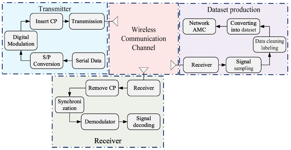
Figure 1. Single-input single-output OFDM signal system diagram.
Ai 06 00323 g001
Figure 2. The structure of the proposed model.
Ai 06 00323 g002
Figure 3. The classification performances of the proposed method and different models, comparing accuracy with different signal datasets.
Ai 06 00323 g003aAi 06 00323 g003b
Figure 4. The scale of the proposed models.
Ai 06 00323 g004
Figure 5. The classification performance of the proposed method and comparing benchmarks with different datasets.
Ai 06 00323 g005aAi 06 00323 g005b
Table 1. The configurations of the proposed algorithm.
AWMN for OFDM Automatic Modulation Classification
Input: IQ signal sequence x (shape: [B, C, T])
Output: Modulation predictions logit (shape: [B, num_classes])
Initialize parameters:
 Adaptive Wavelet blocks, Mamba block, Conv layers, Linear layers
 Hyperparameters: num_wavelet_levels, num_classes, λd = 0.01, λa = 0.01
1. Adaptive Wavelet time-frequency feature extraction:
 a. Conv projection: x = Conv2d(x, kernel = (2,7), out_channels = 64) → [B, 64, T]
 b. Multi-level wavelet decomposition:
 for i in 0 to num_wavelet_levels-1:
  xeven = x[:, :, ::2], xodd = x[:, :, 1::2]
  H = xodd − P(xeven)
  L = xeven + U(H)
 Regularization
  regu_details = λd × mean (abs(H))
  regu_approx = λa × dist (mean(L), mean(x), p = 2)
  regu_sum.append (regu_details + regu_approx)
 x = concatenate ([H, L], dim = 1)
2. Mamba long-term sequence modeling:
 a. Dynamic Δ prediction: Δ = Softplus(W_Δ · SiLU(Conv1d(x, kernel = 4)))
 b. Discrete SSM: A = exp(Δ·A), B = (exp(Δ·A)-I)/(Δ·A)·Δ·B
 c. Parallel scan: x = PScan(A, B·x)
 d. Output projection: x = C·x + D·x_input
3. Classification:
x = AdaptiveAvgPool1d(x, 1) → flatten → Linear → Dropout → logit = Linear(x, num_classes)
Return logit, regu_sum (for total loss: L_total = L_CE + sum(regu_sum))
Table 2. The parameters of the OFDM signal.
Type of ParameterValue
FFT Length256
CP Length64
Frame Length320
Bit Block Size125
1st Message start53
2nd Message start129
Sample per symbol16
Sampling points1024
Carrier frequency4G Hz
Doppler shift800 Hz
Modulation TypeBPSK, QPSK, 8PSK, 16PSK, 4PAM, 16QAM, 32QAM, 64QAM, 128QAM, 256QAM and 512QAM
Table 3. The training accuracy of the models.
ModelsMaximum
Accuracy
(a)
Average
Accuracy
(a)
Maximum
Accuracy
(b)
Average
Accuracy
(b)
Average
Accuracy
(EVAS)
AWMN92.8%62.39%94.1%64.50%75.95%
AWAN92.2%61.66%93.4%63.48%74.38%
MAMC91.4%59.89%92.7%61.79%72.36%
ResNet89.2%57.11%90.8%59.52%68.57%
Transformer88.9%57.05%90.4% 59.85%67.75%
CLDNN89.6%58.67%89.8% 60.42%70.53%
MCNET87.1%56.70%90.1%60.75%68.43%
Disclaimer/Publisher’s Note: The statements, opinions and data contained in all publications are solely those of the individual author(s) and contributor(s) and not of MDPI and/or the editor(s). MDPI and/or the editor(s) disclaim responsibility for any injury to people or property resulting from any ideas, methods, instructions or products referred to in the content.