Article

Scaling Swarm Coordination with GNNs—How Far Can We Go?

by
Gianluca Aguzzi
*,
Davide Domini
,
Filippo Venturini
and
Mirko Viroli
Department of Computer Science and Engineering, Alma Mater Studiorum–Università di Bologna, 40126 Bologna, Italy
*
Author to whom correspondence should be addressed.
AI 2025, 6(11), 282; https://doi.org/10.3390/ai6110282 (registering DOI)
Submission received: 15 September 2025 / Revised: 14 October 2025 / Accepted: 24 October 2025 / Published: 1 November 2025
(This article belongs to the Section AI in Autonomous Systems)

Abstract

The scalability of coordination policies is a critical challenge in swarm robotics, where agent numbers may vary substantially between deployment scenarios. Reinforcement learning (RL) offers a promising avenue for learning decentralized policies from local interactions, yet a fundamental question remains: can policies trained on one swarm size transfer to different population scales without retraining? This zero-shot transfer problem is particularly challenging because the traditional RL approaches learn fixed-dimensional representations tied to specific agent counts, making them brittle to population changes at deployment time. While existing work addresses scalability through population-aware training (e.g., mean-field methods) or multi-size curricula (e.g., population transfer learning), these approaches either impose restrictive assumptions or require explicit exposure to varied team sizes during training. Graph Neural Networks (GNNs) offer a fundamentally different path. Their permutation invariance and ability to process variable-sized graphs suggest potential for zero-shot generalization across swarm sizes, where policies trained on a single population scale could deploy directly to larger or smaller teams. However, this capability remains largely unexplored in the context of swarm coordination. For this reason, we empirically investigate this question by combining GNNs with deep Q-learning in cooperative swarms. We focused on well-established 2D navigation tasks that are commonly used in the swarm robotics literature to study coordination and scalability, providing a controlled yet meaningful setting for our analysis. To address this, we introduce Deep Graph Q-Learning (DGQL), which embeds agent-neighbor graphs into Q-learning and trains on fixed-size swarms. Across two benchmarks (goal reaching and obstacle avoidance), we deploy up to three times larger teams. The DGQL preserves a functional coordination without retraining, but efficiency degrades with size. The ultimate goal distance grows monotonically (15–29 agents) and worsens beyond roughly twice the training size ( 20 agents), with task-dependent trade-offs. Our results quantify scalability limits of GNN-enhanced DQL and suggest architectural and training strategies to better sustain performance across scales.

1. Introduction

Context. The coordination of large-scale multi-agent systems poses fundamental challenges across robotics, artificial intelligence, and distributed systems. As autonomous agents become increasingly prevalent in applications ranging from drone swarms for environmental monitoring [1] to autonomous vehicle fleets [2], as well as intelligent edge-cloud systems [3], the demand for scalable coordination strategies has intensified. These systems must operate under stringent constraints where agents possess only partial, local information, yet must collectively achieve global objectives through decentralized decision making.
Multi-Agent Reinforcement Learning (MARL) [4] has emerged as a promising framework for learning coordination policies in distributed environments. However, a critical limitation emerges in the practical deployment. The current MARL approaches typically learn policies for fixed agent populations during training, while the real-world deployments often require operation with variable agent numbers. This mismatch is evident in search-and-rescue scenarios where drone availability fluctuates due to battery depletion or mechanical failures, or in autonomous vehicle systems that must adapt to varying traffic densities. Retraining policies for each possible agent count is computationally prohibitive and impractical when populations fluctuate dynamically. This scalability challenge is particularly pronounced in the swarm systems, in which homogeneous agents must coordinate through local interactions.
We focused specifically on zero-shot scalability—the capacity of a policy trained on a specific swarm size to maintain functional coordination when deployed with different agent numbers without retraining. This raises the fundamental question of whether coordination strategies learned at one scale can generalize to different population sizes while preserving both functionality and efficiency. To address this challenge, we focused on homogeneous swarm systems operating under centralized training with decentralized execution (CTDE) [5]. Our target systems are characterized by the following: (i) cooperative objectives with collective returns, (ii) homogeneous policies with parameter sharing, (iii) partial observability with time-varying interaction graphs, and (iv) the CTDE training paradigm.
Research Gap. Despite significant advances in MARL, the scalability problem remains largely unresolved. While the existing approaches often address task complexity [6] or communication optimization [7], few directly tackle population scalability. Notable exceptions include mean-field RL [8] and macro-programming abstractions [9]. However, these approaches either impose restrictive assumptions or require domain-specific programming, leaving zero-shot scaling largely unexplored. Graph Neural Networks (GNNs) [10] offer a promising solution to this challenge. The alignment between swarm systems and graph representations is natural. The agents correspond to nodes, interactions form dynamic edges, and GNN message-passing mirrors neighborhood communication patterns. The permutation invariance and variable graph size handling capabilities of GNNs suggest potential for population-level generalization. While the recent work on GNN applications for swarm dynamics [11] shows promise, the specific question of zero-shot scalability—maintaining both functional coordination and efficiency across swarm sizes without retraining—remains unexplored.
Contribution. This paper addresses the research gap above through an empirical investigation of GNN scalability in swarm coordination. Our key research question is: To what extent can GNN-based policies trained at a fixed swarm size preserve functional coordination and maintain efficiency when deployed at different population sizes without retraining? To investigate this question, we introduce Deep Graph Q-Learning (DGQL), a MARL algorithm that integrates GNNs into deep Q-learning for swarm coordination. DGQL operates under the CTDE paradigm, utilizing GNNs to process dynamic agent-neighbor interaction graphs during training while enabling fully decentralized execution through local message passing. Our study specifically focuses on homogeneous swarms performing 2D navigation tasks, providing a controlled setting to isolate the effects of GNN-based policy scaling rather than addressing more complex or heterogeneous domains.
The main contributions of this work are threefold as the following:
  • Algorithmic contribution: We formalize DGQL, integrating GNN architectures into Q-learning to process dynamic agent-neighbor interaction graphs while maintaining permutation invariance and variable neighborhood handling capabilities.
  • Empirical evaluation: We demonstrate DGQL’s effectiveness on two cooperative benchmark tasks—goal reaching and obstacle avoidance—establishing successful learning of decentralized coordination policies under the CTDE paradigm.
  • Scalability analysis: We provide the first systematic quantification of zero-shot scalability for GNN-based swarm policies, evaluating models trained on ten-agent swarms when deployed with populations up to three times larger, thereby revealing task-dependent efficiency degradation patterns.
Our experimental findings demonstrate near zero-shot scalability: policies trained with ten agents preserve functional coordination without retraining, yet efficiency declines progressively as swarm size increases beyond training conditions. Across evaluations spanning 15–29 agents, the terminal distance to the goal increases monotonically with the team size, with particularly steep degradation once the swarm exceeds approximately twice the training size (≈20 agents). While GNNs successfully prevent catastrophic failure across different scales, efficiency degrades steadily and accelerates beyond twice the training size, thus providing a realistic baseline for deployments with variable yet constrained swarm populations.
Paper Structure. This paper is organized as follows: Section 2 positions our work within the existing literature; Section 3 provides essential background on swarm modeling and multi-agent reinforcement learning; Section 4 presents the DGQL algorithm; Section 5 describes our experimental methodology and results; Section 6 discusses implications and future research directions. Finally, Section 7 concludes and outlines future works.

2. Related Work

The scalability of multi-agent reinforcement learning (MARL) remains a central challenge. We focus on zero-shot scalability in swarm coordination with Graph Neural Networks (GNNs), and position our study within three complementary strands: scaling in agent count, scaling in state/action complexity, and CTDE with learned communication.

2.1. Scalability in the Number of Agents

Independent learners face non-stationarity and coordination issues as agent counts grow [12,13]. Mean-field MARL mitigates this via population distributions, enabling large-scale training but relying on strong homogeneity assumptions [8,14,15]. Parameter sharing helps but can limit behavioral diversity [16]. To handle variable populations, recent work uses GNNs and permutation-invariant/equivariant models to generalize across team sizes [17,18,19], building on graph-based policies that naturally process variable neighborhoods [20,21,22].

2.2. Scalability in State and Action Spaces

Deep function approximation (e.g., MADDPG) addresses high-dimensional observations or actions under CTDE [23], while value decomposition (VDN, QMIX, QTRAN, QPLEX, and QFIX) enables decentralized execution via structured mixing [24,25,26,27,28]. Partial observability is tackled with centralized critics and attention for selective aggregation [29,30]. Permutation-invariant/equivariant architectures further improve generalization across agent permutations and configurations [31,32].

2.3. Decentralized Execution and Communication

CTDE is the prevailing paradigm for practical deployment [33], with recent work exploring degrees of centralization during training (e.g., CADP) [34]. Learned communication improves coordination via differentiable channels, attention, and sparsity, including under wireless constraints [35,36,37,38]. Transformers and routing mechanisms have been proposed for long-range information flow [39,40], while GNN-based communication scales to large teams with efficiency and safety guarantees [41,42].

2.4. Positioning of Our Work

We study zero-shot population scaling with GNNs in value-based MARL under CTDE, without training on multiple team sizes. Compared to mean-field methods [8] and GNN-based population-transfer approaches [17], we quantify how performance degrades as deployment sizes diverge from training. Our DGQL complements permutation-invariant models [18,32] and communication-centric methods [40,42], providing an empirical baseline on the limits of zero-shot scalability in swarm coordination.

3. Background

In this section, we provide an overview of the key concepts and models that underpin our approach. In particular, we discuss a formalization of the swarming model, the multi-agent reinforcement learning framework, and the graph neural network model.

3.1. Swarming Model Formalization

The system we aim to model consists of a set of autonomous agents that collaborate to accomplish a collective task through a sequence of local actions. To formalize this interaction between the agents and their environment, we adopt the SwarMDP model [5], which is a specialized subclass of DecPOMDP models [43].
SwarMDP extends the classic Markov Decision Process (MDP) framework to multi-agent systems, where all agents are homogeneous—that is, they possess identical capabilities for perception and interaction. This homogeneity is crucial for our scalability investigation, as it enables parameter sharing and coordination learning that can potentially generalize across different swarm sizes. In this model, the system is described as a tuple comprising a swarming agent a and an environment E . The agent prototype is defined as a tuple: a = ( S , O , A , ρ , π ) , where:
  • S represents the set of environment states, which are not directly observable by the agents.
  • O denotes the set of observations available to the agents.
  • A is the set of actions that an agent can perform to interact with the environment.
  • ρ : O × A R defines the reward function, mapping observations/actions pairs to rewards.
  • π is the agent’s local policy—the collective interaction of these individual policies results in the emergent swarm behavior.
The environment coordinates the interactions of multiple instances of this agent prototype.
These swarming agents operate in an environment defined by E = N , a , T , Y , where:
  • N N is the number of agents in the swarm.
  • a denotes a swarming agent, as defined earlier.
  • T : S N × A N S N is the global state transition function, mapping the current global state (an element of S N ) and a joint action (an element of A N ) to the next global state.
  • Y : S N O N defines the observation model that provides each agent with its local observations derived from the global state.
The whole evolution in one step can be represented as a sequence of functions as the following:
S N Y O N π A N T S N .
This functional sequence captures the complete swarm decision cycle: from global state to local observations, from observations to joint actions, and from joint actions back to the next global state. Note that, for the sake of simplicity, this model assumes that time evolves in discrete, synchronous time steps. However, in real-world deployments, the evolution may be asynchronous, with some agents potentially executing no-operation (nop) actions during certain time steps. In what follows, we denote by o i O the observation received by agent i, by s i S its hidden state, and by a i A the action chosen by agent i. For clarity, the superscript t denotes the values at time step t, so that for each agent i, o i t represents the observation at time t, r i t represents the reward received at time t, and a i t represents the action taken at time t.
Similarly, the boldface versions indicate the global quantities for the entire swarm. The following are examples:
o t = ( o 1 t , , o N t ) , r t = ( r 1 t , , r N t ) , a t = ( a 1 t , , a N t ) .
SwarMDP models do not explicitly capture the communication between agents, which is essential for coordination in our study. To address this limitation, we extend the SwarMDP by introducing a neighborhood function that maps each agent index to the set of indices corresponding to the agents within its communication range. Formally, for each agent i, with i { 1 , , N } , its neighborhood at time t is defined as the following
N t ( i ) { 1 , , N } ,
where N t ( i ) returns the set of indices of agents that are considered neighbors at time t. This neighborhood relationship naturally changes as agents move or as communication conditions vary. With this neighborhood function, we can naturally construct a graph representation of the system. A graph is defined as G t = ( V , E t ) , where V is the set of nodes and E t is the set of edges. Given an extended SwarMDP ( a , E , N ) , for each time slot t, a graph can be computed as follows:
V = { 1 , , N } , E t = { ( i , j ) i V , j N t ( i ) } .
This dynamic graph representation will prove essential for our GNN-based approach, as it captures the time-varying communication topology that agents must navigate for coordination. To streamline exposition, we reuse N both for the number of agents and (with a subscript) for the neighborhood function N t ( · ) . The context disambiguates the meaning.
Having formalized the swarm dynamics and graph representation, we proceed to establish the reinforcement learning framework needed to learn coordination policies. Our approach operates under standard assumptions that the homogeneous agents with shared policy parameters, partial observability with local communication, and centralized training with decentralized execution.

3.2. Multi-Agent Reinforcement Learning

After formalizing the swarm model, we need a learning mechanism that enables agents to discover effective coordination policies. A widely used strategy for sequential decision making is Reinforcement Learning (RL) [44]. RL has gained prominence due to its successes across diverse domains—from mastering complex games like Go, Chess, StarCraft, and Dota2 [44,45,46,47] to driving advanced robotics applications [48,49].
In this work, we focus on Multi-Agent Reinforcement Learning (MARL), which extends RL to scenarios in which multiple agents interact and learn concurrently [12]. MARL encompasses several dimensions, such as the task nature (cooperative, competitive, and mixed), the information structure (fully observable, partially observable, and decentralized), and the learning paradigm (centralized training with decentralized execution, decentralized training with decentralized execution, and among others). Since our system is modeled as a SwarMDP, we assume a cooperative task with partially observable information, as agents can only perceive their local environments.
In this context, the goal of MARL is to learn an optimal homogeneous policy for the swarming agents. Here, “optimal” refers to maximizing the expected sum of collective rewards, which encourages agents to coordinate their actions for the benefit of the entire swarm rather than pursuing purely individual objectives. The collective return is defined as the following:
G = t = 0 H 1 i = 1 N r i t + 1 ,
where H is the time horizon (number of decision steps) in an episode. Thus, the objective is to determine a policy π * that maximizes the expected collective return, written as the follwoing:
π * = arg max π E π G .
One effective method to approach MARL is by extending the classic Q-learning algorithm to the multi-agent setting. Q-learning [50], a model-free RL algorithm, learns the quality (or Q-value) of state-action pairs. The Q-value represents the expected return from taking a given action in a specific state and thereafter following a given policy. For agent i at time t in our SwarMDP model, the Q-value is defined as the following:
Q i π , t ( o i t , a i t ) = E π k = t T γ k t r i k | o i t , a i t .
This formulation can be extended into deep settings, where the Q-value is approximated by a neural network, giving rise to deep Q-learning (DQL) [51]. The neural network function approximation becomes essential when dealing with high-dimensional observation spaces typical in realistic swarm environments. In DQL, the Q-value approximation is represented as Q ( · ; θ ) with network parameters θ . The corresponding loss function is defined using the mean squared error between the predicted Q-value and a target Q-value. Using the convention that rewards are observed after taking action a i t and indexed as r i t + 1 , the loss is as the following:
L ( θ ) = E π Q i π , t ( o i t , a i t ) r i t + 1 + γ max a Q i π , t + 1 ( o i t + 1 , a ) 2 .
where E denotes the expectation. The parameters are updated via gradient descent on this loss function, while a replay buffer–denoted as a tuple ( B , B ) with B representing the buffer and B the batch size–stores past experiences. A sampled mini-batch of experiences for agent i is given by:
{ ( o i t j , a i t j , r i t j + 1 , o i t j + 1 ) } j = 1 B ,
where t j represents different time steps in the agent’s experience history.
A straightforward strategy in SwarMDP is to apply independent Q-learning [13], where each agent learns its own policy using only local observations. However, independent learning can suffer from non-stationarity issues as multiple agents simultaneously adapt their policies. This work adopts a CTDE scheme, which addresses these challenges. During training, a centralized buffer stores the observations, actions, rewards, and subsequent states for all agents, enabling experience sharing [16]. In CTDE, agents learn a global policy by considering the entire system’s information during training, but during execution, each agent relies solely on its local perception [52,53].

3.3. Graph Neural Networks

Graph Neural Networks (GNNs) represent a class of deep learning models specifically designed for processing data structured as graphs [10]. They are particularly well-suited for swarm coordination because the dynamic communication topology naturally forms a graph where agents are nodes and communication links are edges. Given a graph G t , the primary objective of a GNN is to learn a vector representation, or embedding, h v R d for each node v V . This embedding aims to capture both the node’s intrinsic features and the contextual information derived from its local neighborhood structure within the graph.
GNNs achieve this through a mechanism known as message passing [54], often implemented across multiple layers. This process mimics natural communication patterns in swarms where agents exchange information with their neighbors. Let K be the total number of message passing layers. The process iteratively updates node embeddings by aggregating information from their neighbors. Let h v ( k ) denote the embedding of node v at layer k, where k { 0 , , K } . The initial embedding h v ( 0 ) is typically initialized with the node’s input features, f v (derived from the agent’s observation o v ).
For each subsequent layer k = 1 , , K , the update process can be generally described in three steps as the following:
  • Message Computation: For each edge ( u , v ) E t , a message m u v ( k ) is computed. This message typically depends on the embeddings of the source node u and the target node v from the previous layer, h u ( k 1 ) and h v ( k 1 ) , potentially incorporating edge features e u v if available. This step is governed by a learnable message function ψ ( k ) as the following:
    m u v ( k ) = ψ ( k ) h u ( k 1 ) , h v ( k 1 ) , e u v .
  • Message Aggregation: Each node v aggregates the incoming messages from its neighbors. Let N G t ( v ) = { u V ( u , v ) E t } denote the set of neighbors of node v in graph G t . The aggregation function ( k ) (e.g., sum, mean, and max) combines the messages into a single vector a v ( k ) as the following:
    a v ( k ) = u N G t ( v ) m u v ( k ) .
    Note that some formulations aggregate messages based on m v u ( k ) (messages to neighbors) or use slightly different definitions. The core idea remains aggregating neighborhood information.
  • Embedding Update: The embedding of node v for the current layer, h v ( k ) , is computed by combining its previous embedding h v ( k 1 ) with the aggregated message a v ( k ) . This update is performed using a learnable update function ϕ ( k ) (often a neural network layer like an MLP, potentially combined with activation functions like ReLU) as the following:
    h v ( k ) = ϕ ( k ) h v ( k 1 ) , a v ( k ) .
After K layers of message passing, the final node embeddings are { h v ( K ) v V } . With K layers, each agent’s embedding contains information from agents up to K communication hops away, enabling coordination across extended neighborhoods without requiring direct long-range communication.
The entire GNN computation can be represented as a function that maps the initial node features f = { f v } v V and the graph structure G t to the final embeddings, parameterized by the learnable weights θ encompassing all ψ ( k ) , ( k ) , ϕ ( k ) as the following:
GNN ( f , G t , θ ) = h v ( K ) : v V .
These final embeddings h v ( K ) encapsulate multi-hop neighborhood information (up to K hops) and serve as rich feature representations for downstream tasks, such as predicting Q-values in our reinforcement learning context. Crucially for our scalability investigation, GNNs offer permutation invariance (agent ordering does not affect output) and can handle variable graph sizes, potentially enabling policies to generalize across different swarm sizes.
A key property that enables this scalability is the neighborhood invariance of GNNs in which each agent’s embedding depends only on its local neighborhood structure and features, not on the global graph size or the identities of agents outside its K-hop neighborhood. Formally, for an agent v in a graph G , its final embedding h v ( K ) is determined solely by the subgraph G v ( K ) containing v and all nodes within K hops, along with their features and connectivity. This means that if two agents in different swarms have identical K-hop neighborhoods (same relative positions, features, and local connectivity patterns), they will produce identical embeddings regardless of what happens elsewhere in their respective swarms. This locality property is what allows GNN-based policies trained on small swarms to potentially operate on larger swarms without retraining, as long as the local neighborhood patterns remain consistent.

4. Deep Graph Q-Learning

This paper introduces and evaluates Deep Graph Q-learning (DGQL), a MARL tailored for swarm coordination tasks. DGQL integrates GNNs into the Deep Q-Learning (DQL) [51] framework to explicitly model and leverage the relational structure inherent in agent interactions. This integration is motivated by the observation that traditional DQL treats agents as independent entities, failing to capture the collaborative dependencies essential for effective swarm coordination. By representing agent interactions as dynamic graphs and using GNNs for Q-value estimation, DGQL can learn coordination policies that generalize across different swarm topologies and sizes—a critical requirement for scalable deployment. The core innovation of DGQL lies in its adaptation of the standard DQL components to incorporate graph-structured reasoning as the following:
  • Graph-based State Representation: Instead of treating agents independently based solely on local observations, DGQL represents the swarm’s state at time t as a graph G t = ( V , E t ) , where nodes V = { 1 , , N } correspond to agents and edges E t represent neighbor relationships (e.g., based on communication range or proximity, determined by N t ). The initial node features f t are derived from the agents’ local observations o t = { o 1 t , , o N t } .
  • Graph Q-Network (GQN): The standard Deep Q-Network is replaced by a GQN. This network takes the graph G t and node features o t as input and computes Q-values for each agent i V and each possible action a A . The GQN architecture first employs GNN layers (as described in Section 2) that perform message passing to compute node embeddings h i ( K ) for each agent i. These embeddings encode information about the agent’s state and its K-hop neighborhood within the graph G t . Then, a final output layer maps each agent’s final embedding h i ( K ) to its action-value estimates: Q ( o t , G t ; θ ) i [ a ] = Q i ( h i ( K ) , a ) for each a A , where θ represents the learnable parameters of the entire GQN. Critically, the GQN parameters θ are shared across all agents, promoting homogeneous behavior and facilitating learning from collective experience.
  • Centralized Training with Graph Experience Replay: DGQL operates within a CTDE paradigm. During training, experiences are stored in a replay buffer B . Each experience tuple contains the full graph representation and collective information from a transition: ( G t , o t , a t , r t + 1 , G t + 1 , o t + 1 ) , where a t is the joint action and r t + 1 is the vector of individual rewards. Storing the graph structure allows the GQN to learn from the system’s interaction topology during optimization.

4.1. Centralized Training

The training objective is to minimize the standard DQL loss function, adapted for the multi-agent graph context as the following:
L ( θ ) = E ( G t , o t , a t , o t + 1 , G t + 1 , r t + 1 ) B i = 1 N y i Q ( o t , G t ; θ ) i [ a i t ] 2
where [ a i t ] denotes the Q-value corresponding to the action taken by agent i at time t. The target value y i for agent i is calculated using a target network Q with parameters θ as follows:
y i = r i t + 1 + γ max a A Q ( o t + 1 , G t + 1 ; θ ) i [ a ]
where the parameters θ are updated via gradient descent on this loss. The target network parameters θ are periodically updated with the main network parameters θ to stabilize learning, as standard in DQL. The overall training procedure is detailed in Algorithm 1. At each step within an episode the following are considered:
Ai 06 00282 i001 
The current swarm state is represented as a graph G t .
Ai 06 00282 i002 
The GQN computes Q-values q for all agents.
Ai 06 00282 i003 
A joint action a is selected (e.g., using an ϵ -greedy strategy independently for each agent based on its Q-values).
Ai 06 00282 i004 
The transition, including the graph structures, is stored in the replay buffer B .
Ai 06 00282 i005 
A batch is sampled from B .
Ai 06 00282 i006 
The GQN parameters θ are updated via a gradient descent step on the loss L ( θ ) .
The use of GNNs allows efficient batch processing of graph data, making the centralized training phase computationally feasible even for moderately sized swarms.

4.2. Decentralized Execution

During execution, DGQL operates in a fully decentralized manner. Each agent i observes only its local state o i t and exchanges messages with neighbors j N t ( i ) within the communication range. Using the pre-trained graph Q-network with shared parameters θ , each agent builds a local ego-graph G t i consisting of itself and current neighbors, then applies the GNN to compute action-values from local features and neighbor messages.
Decentralized execution follows a K-round message passing protocol per environment step as follows: neighbors exchange d-dimensional embeddings h ( k 1 ) , then each agent updates h ( k ) via Equations (10)–(12). The final embedding h i ( K ) aggregates information up to K hops away, enabling each agent to select actions based on a i t = arg max a A Q i ( h i ( K ) , a ) , where Q i ( · , · ) represents the output layer mapping embeddings to Q-values. Critically, this computation depends only on local neighborhood size k and message width d, not the global swarm size N , ensuring scalability. We set K = 1 in our experiments to minimize communication rounds while preserving immediate neighborhood awareness. More formally, we can characterize the resulting decentralized policy as follows: at time step t, each agent i forms its ego-graph G t i over nodes { i } N t ( i ) . With K GNN layers and shared parameters θ , it computes h i ( K ) = GNN ( f , G t i ; θ ) and selects actions greedily. This policy is permutation invariant with respect to agent indexing and has runtime complexity independent of global population size, which are key properties that enable the zero-shot scalability we investigate in this work.
Algorithm 1 Deep graph Q-learning (DGQL)
1:
Initialize: env E , exploration rate ε , graph Q-network Q ( · ; θ ) , target network Q ( · ; θ ) Q ( · ; θ ) , replay buffer B
2:
for episode τ = 1  to  T max  do
3:
   Get initial obs o 0 ; set t 0
4:
   while not terminal do
5:
       Build graph G t from neighborhood N t                                                          Ai 06 00282 i001
6:
        q Q ( o t , G t ; θ )                                                                                                 Ai 06 00282 i002
7:
        a ε -greedy policy based on q                                                                      Ai 06 00282 i003
8:
       Execute a , observe o t + 1 , r t + 1
9:
       Build G t + 1 from N t + 1
10:
     Store ( G t , o t , a , r t + 1 , G t + 1 , o t + 1 ) in B                                                                  Ai 06 00282 i004
11:
     Sample batch of experiences from B                                                            Ai 06 00282 i005
12:
     For each agent i: y i = r i t + 1 + γ max a A Q ( o t + 1 , G t + 1 ; θ ) i [ a ]
13:
     Update θ to minimize i Q ( o t , G t ; θ ) i [ a i t ] y i 2                                          Ai 06 00282 i006
14:
     Every C steps: θ θ
15:
      o t o t + 1 ; t t + 1
16:
   end while
17:
end for
Notation in Table 1, the circles Ai 06 00282 i001Ai 06 00282 i006 refer to the steps described in the text.
Finally, the Algorithm 2 summarizes the decentralized forward pass executed at each environment step.
Algorithm 2 Decentralized DGQL execution (per environment step)
1:
Each agent i gathers local observation o i t and initializes h i ( 0 ) f ( o i t )
2:
for  k = 1 to K do
3:
   Agent i sends h i ( k 1 ) to neighbors j N t ( i ) and receives { h j ( k 1 ) } j N t ( i )
4:
   Agent i aggregates messages: a i ( k ) j N t ( i ) ψ ( k ) ( h j ( k 1 ) , h i ( k 1 ) , e j i )
5:
   Agent i updates embedding: h i ( k ) ϕ ( k ) ( h i ( k 1 ) , a i ( k ) )
6:
end for
7:
Agent i computes action-values q i Head ( h i ( K ) ) and selects action (greedy during evaluation)
Notation in Table 1
Table 1. Notation used in Algorithms 1 and 2.
Notation Summary
General
E Environment
τ , t Episode and time step indices
T max Maximum number of training episodes
ϵ , γ Exploration rate and discount factor
B Replay buffer
A Action space
CTarget network update frequency
Networks and Learning
Q ( · ; θ ) , Q ( · ; θ ) Graph Q-network and target network
y i TD target for agent i
q Q-values for all agents
q i Q-values for agent i
Head ( · ) Output layer mapping embeddings to Q-values
Observations and Graphs
o t Joint observations at time t
o i t Local observation of agent i at time t
G t = ( V , E t ) Interaction graph at time t
N t ( i ) Set of neighbors of agent i at time t
Agents and Messages
i , j Agent and neighbor indices
h i ( k ) Embedding of agent i at layer k
f ( · ) Feature extraction function
ψ ( k ) ( · ) , ϕ ( k ) ( · ) Message and update functions at layer k
Aggregation operator (e.g., sum, mean, max)
a i ( k ) Aggregated message for agent i at layer k
e j i Edge features between agents j and i
KNumber of GNN layers (message passing rounds)
kCurrent layer index
Actions and Rewards
a Joint action
r t + 1 Rewards at time t + 1

4.3. Complexity and Communication Cost

For a graph with | V | = N nodes and | E t | edges, a single forward pass of a K-layer message passing GNN with hidden width d has time complexity O K ( | V | d 2 + | E t | d ) . Under a k-nearest neighbor graph, | E t | = O ( k N ) . During decentralized execution, K sequential communication rounds per environment step are required (one per GNN layer), yielding an amortized per-agent communication cost of O ( K k d ) messages. Figure 1 empirically validates the proposed cost analysis, showing that the measured trends closely follow the theoretical estimates. In some cases, the inference time is slightly higher, likely due to implementation details in PyTorch Geometric (v2.5.3), but the deviation remains negligible.

5. Evaluation

To verify if the proposed approach is able to generalize across different swarm sizes and to perform different swarming behaviors, we designed a set of tasks for the swarm of agents to perform. We restrict our evaluation to simple, as they allow systematic investigation of scalability without confounding factors from task-specific dynamics. Moreover, these tasks are commonly adopted in swarm robotics as canonical benchmarks. For instance, Brambilla et al. [55] identify goal-seeking and obstacle avoidance as fundamental behaviors underlying flocking and foraging, and several other studies have employed similar setups to evaluate decentralized control and scalability [1,56,57]. The experiments described below are fully available and reproducible in the repository (https://github.com/domm99/experiments-2025-marl-scalability-for-swarming-behaviors, accessed on 26 October 2025). In the following, we describe the tasks, the experimental setup, and the results obtained.

5.1. Tasks

To evaluate the coordination capabilities and scalability of the learned policies, we designed two benchmark tasks within a simulated 2D continuous environment. These tasks require agents to navigate towards a common goal while managing spatial interactions, both among themselves and potentially with environmental obstacles. The reward structures are designed to elicit specific coordinated behaviors.
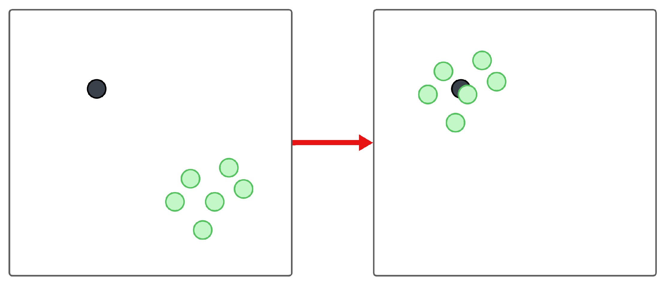
The primary objective of this task (Figure 2) is for a swarm of agents, starting from randomized positions, to collectively converge towards a predefined target location g R 2 within the environment. Let p i R 2 denote the position of agent i at a given time step, and let N be the total number of agents in the swarm. The Euclidean distance of agent i from the goal is given by d i = p i g 2 . The immediate reward r i received by agent i is defined as the negative distance to the goal as the following:
r i = d i .
This reward function directly incentivizes agents to minimize their distance to the target g. Since the objective in MARL is typically to maximize the sum of rewards over time, this formulation encourages agents to reach the goal as quickly as possible. Although inter-agent collisions are not explicitly penalized in this task, they inherently impede progress towards the goal, thus indirectly promoting the emergence of coordinated, collision-averse navigation strategies to maximize the collective return. The shared reward for the swarm is the sum of individual rewards, i = 1 N r i .

Obstacle Avoidance (Figure 3)

This task (Figure 3) extends the Go to Position scenario by introducing a static, circular obstacle into the environment. Agents must not only navigate towards the goal g but also actively avoid colliding with the obstacle. Let o R 2 be the center position of the obstacle, and let d o i = p i o 2 be the Euclidean distance between agent i and the obstacle center. We introduce a penalty threshold distance, d t h r e s h , representing a safety margin around the obstacle (e.g., obstacle radius plus agent radius or a slightly larger buffer). The reward function for agent i is modified to include a penalty term for proximity to the obstacle as follows:
r i = d i α · max ( 0 , d t h r e s h d o i )
where α is a positive weighting factor that controls the magnitude of the penalty for violating the safety distance d t h r e s h . The max ( 0 , · ) operation ensures that the penalty is only applied when the agent is closer to the obstacle than the threshold distance ( d o i < d t h r e s h ) and increases linearly as the agent gets closer. In our experiments, we set α = 2.5 . This value was chosen to impose a significant penalty for approaching the obstacle, encouraging agents to prioritize safety and find alternative paths to the goal when necessary. This task presents a more complex coordination challenge, requiring agents to dynamically balance goal-seeking behavior with reactive obstacle avoidance, all while maintaining sufficient separation from other agents. The collective objective remains the maximization of the sum of these individual rewards.
Figure 3. The Obstacle Avoidance task. The agents (green dots) must reach the target (black dot) while navigating around a static obstacle (red dot).
Ai 06 00282 g003

5.2. Experimental Setup

We implement the tasks in a 2D multi-agent simulator built on VMAS [58], using PyTorch [59] and PyTorch Geometric [60] for differentiable graph processing. Policies are parameter-shared across agents and realized by a graph Q-network (GQN) comprising a single graph attention (GAT) layer with 32 hidden units and dropout 0.1, followed by a two-layer MLP head (32 units per layer, ReLU activations). Hyperparameters are summarized in Table 2.
Each agent i receives an observation vector o i R 6 = [ x i , y i , v x , i , v y , i , g x , g y ] , namely its position, velocity, and the goal position. The action space consists of 9 discrete 2D translation primitives.
The environment is a 2 × 2 m square (coordinates normalized to a local frame). During training, the goal is fixed at g = ( 0.8 , 0.8 ) , while the initial positions of the agent are sampled near ( 1.5 , 1.5 ) . The fixed goal position design choice serves a specific methodological purpose: by maintaining a consistent target location, we isolate the scalability question from goal generalization, allowing us to focus exclusively on whether learned coordination patterns transfer across different swarm sizes. The specific goal position ( 0.8 , 0.8 ) creates a non-trivial coordination scenario requiring agents to navigate around obstacles (in the obstacle avoidance task) and converge from dispersed initial positions, thus capturing essential swarm coordination challenges while maintaining experimental control. Episodes last at most 100 steps. At the beginning of each step, we additively perturb the agent positions with a Gaussian noise ϵ N ( μ , σ 2 ) with μ = 0.6 and σ = 0.4 . The Obstacle Avoidance task includes a circular obstacle centered at o = ( 0.1 , 0.1 ) with radius R = 0.2 m.
Training uses N = 10 agents for 1000 episodes under a dynamic communication graph induced by the k-nearest neighbors, recomputed at every step. In this way, each agent communicates only with its five closest neighbors, simulating a realistic setting where agents do not have global communication but interact only with a limited subset of peers. The choice of k = 5 neighbors represents a balance between coordination capability and computational efficiency as it provides each agent with sufficient local neighborhood information to coordinate effectively (enabling multi-agent formation behaviors) while maintaining tractable communication overhead that scales linearly with agent count rather than quadratically as in fully-connected topologies. This parameter choice aligns with biological swarm studies showing that effective collective behaviors often emerge from sparse local interactions [61], and ensures that our approach remains applicable to resource-constrained robotic platforms where communication bandwidth is limited. Optimization is performed with Adam (learning rate 10 3 ), a replay buffer of size 10 6 , and mini-batches of size 32. We apply DGQL with discount γ = 0.99 and update the target network every 200 steps. Exploration follows an ε -greedy policy with exponential decay the following:
ε ( τ ) = max ε min , ε 0 exp ( λ τ ) , ε 0 = 1 , ε min = 0.01 , λ = 10 3 ,
where τ is the training episode index. We log per-episode cumulative reward and average TD loss. All experiments are repeated across multiple random seeds to assess robustness.
For zero-shot evaluation, we vary the swarm size from 15 to 30 agents without retraining. The goal and obstacle configurations match training. The initial agent positions are randomized. We select the best checkpoint by validation return and report two metrics: (i) terminal mean distance to goal, d ¯ T = 1 N i = 1 N p i T g 2 , and (ii) obstacle-collision frequency, computed as the total number of pairs ( i , t ) such that p i t o 2 R across the episode. During evaluation, execution is fully decentralized as in Algorithm 2 with K = 1 , requiring a single neighbor-embedding exchange per step and no access to the global state. Beyond efficiency, choosing K = 1 is behaviorally motivated. It matches the locality assumption of classical self-organization models of collective motion—most notably Reynolds’ Boids [61]—where agents react to instantaneous, 1-hop neighbor cues (separation, alignment, and cohesion). In these models, coordination emerges because local reactions are applied at every step; information propagates over time through the swarm’s dynamics rather than via explicit multi-hop message passing in a single step. Since our goal is to emulate such minimal reactive coordination, we fix K = 1 so that each decision uses only immediate neighbor information with a single exchange. This preserves the intended local-rule prior, avoids oversmoothing from multi-hop aggregation, and keeps latency and bandwidth minimal for deployment.

Reproducibility

All code to reproduce environments, training, and evaluation, including configuration files and scripts to regenerate figures and summary statistics, is provided in the companion repository. We fix seeds for simulators, framework backends, and data loaders and log all hyperparameters (Table 2).

5.3. Results

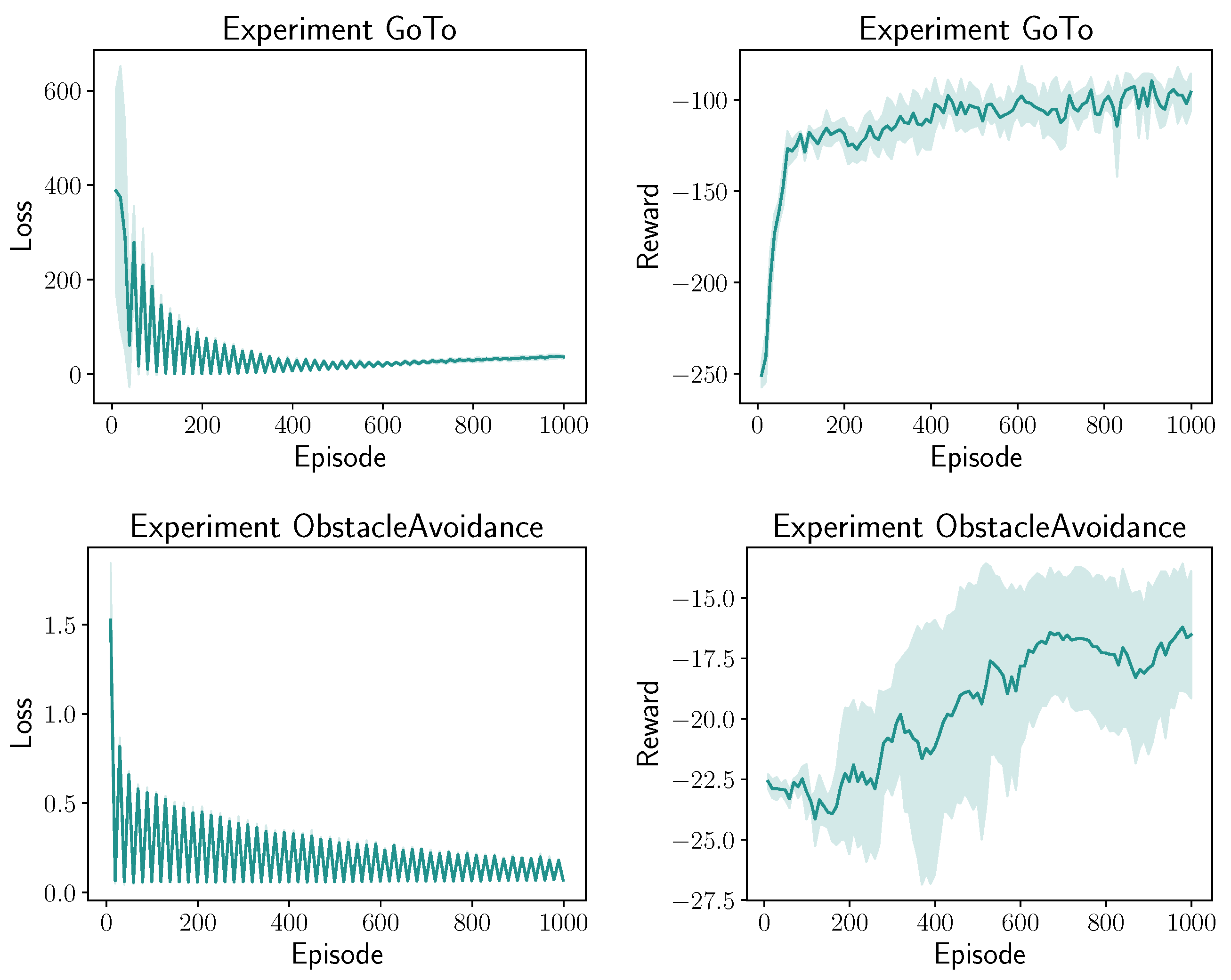
We now present the empirical results that address the research question posed in Section 1. The analysis proceeds in two parts: First, we report training dynamics to verify that DGQL learns stable policies (loss and cumulative return; Figure 4). Second, we evaluate zero-shot population scaling by deploying the learned policies on larger swarms without retraining, summarizing performance with terminal mean distance to the goal and, for Obstacle Avoidance, obstacle-collision counts (Figure 5). To qualitatively assess emergent spatial organization as team size grows, we complement scalar metrics with KDE visualizations of agent trajectories (Figure 6). Unless stated otherwise, results aggregate multiple seeds per configuration, following the protocol in Section 5, and execution is fully decentralized with one message-passing round per step (Algorithm 2).
At a high level, DGQL policies trained on ten agents transfer functionally to larger teams across the tested sizes (15–29 agents, i.e., about 1.5–3 times the training), preserving coordinated behavior and safety (near-zero obstacle collisions). Efficiency declines with increasing population, with task-dependent trade-offs. The following subsections detail learning curves and zero-shot scaling outcomes.

5.3.1. Training Results

The training phase results are summarized in Figure 4 for both the Go to Position (top) and the Obstacle Avoidance tasks (bottom). In both tasks, a clear downward trend in the average loss and a corresponding upward trend in the cumulative reward are observed, which indicates effective learning. Notably, the periodic spikes in loss correspond to the updates of the target network, temporarily degrading performance before subsequent improvement.
For the Go to Position task, learning becomes evident after approximately 100 episodes, whereas the Obstacle Avoidance task requires around 800 episodes to achieve comparable performance. This delay reflects the increased complexity of integrating goal attainment with obstacle avoidance. Moreover, the reward for the Obstacle Avoidance task exhibits greater variability, particularly during the mid-training phase. This variability might suggest potential challenges, such as catastrophic forgetting, where agents could focus on reaching the goal at the expense of obstacle avoidance. Nonetheless, the eventual reduction in standard deviation indicates that the model learns to balance these competing objectives effectively.

5.3.2. Testing Results

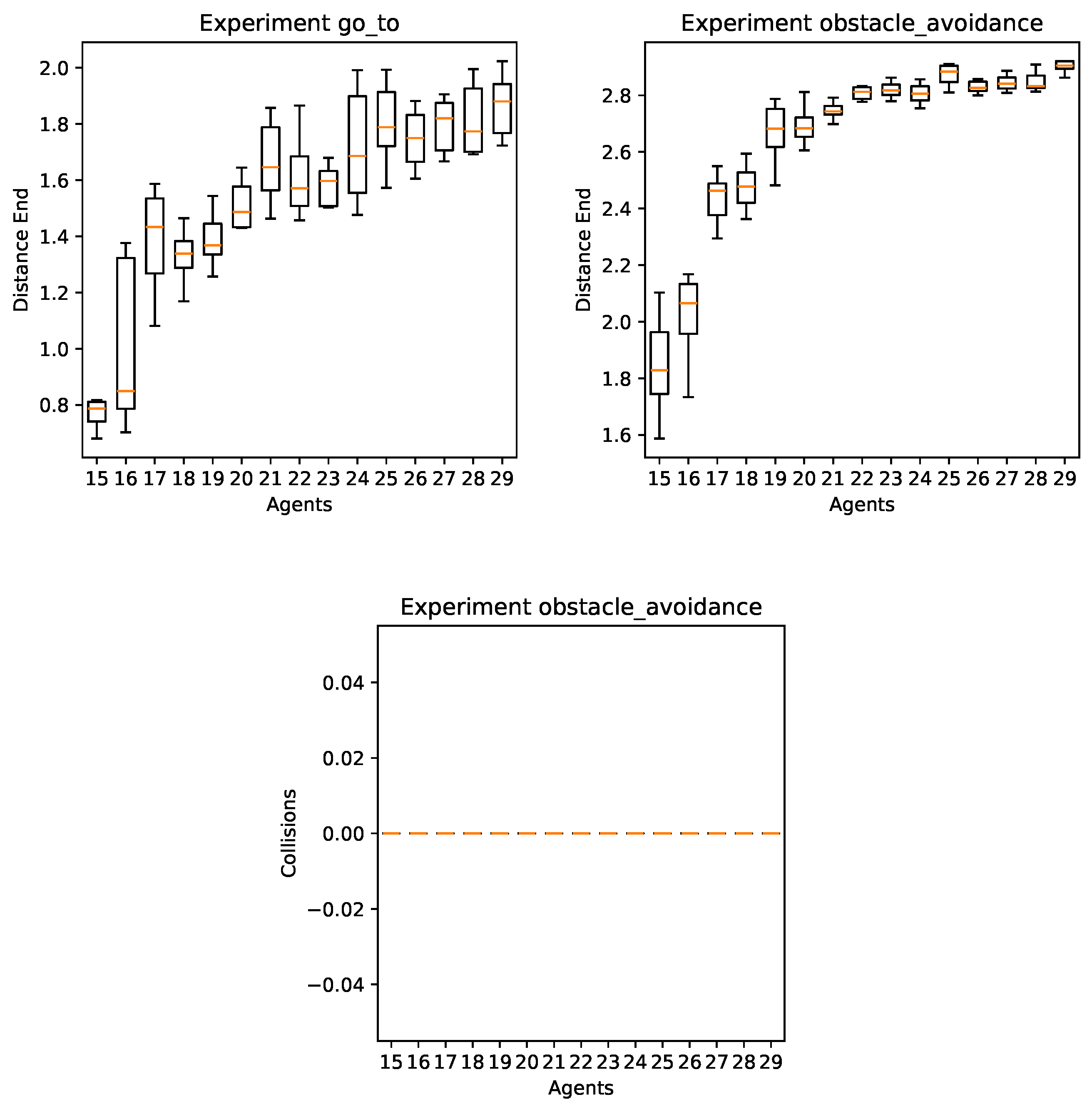
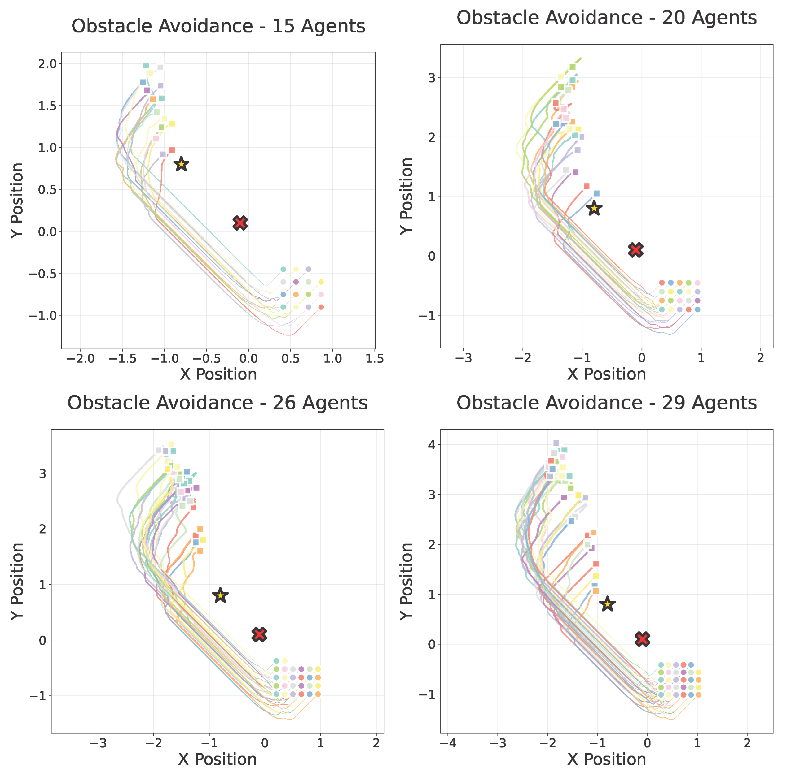
The testing phase results are summarized in Figure 5 and Figure 6 for both tasks. Figure 7 shows example trajectories of agents in the Obstacle Avoidance task for different swarm sizes to illustrate how agents navigate around the obstacle while moving towards the goal and how this behavior changes with swarm size. In Figure 5, the box plots illustrate the distribution of the average distance from the goal at the end of each episode (left and center panels) and the number of collisions with obstacles (right panel) across eight seeds. These results are derived from the best models identified during training, i.e., the models exhibiting the highest cumulative reward.
For the Go to Position task, terminal distance increases monotonically with swarm size across the evaluated configurations (15, 20, 25, and 29 agents), indicating a consistent efficiency degradation as team size grows, with a sharper increase once exceeding twice the training size.
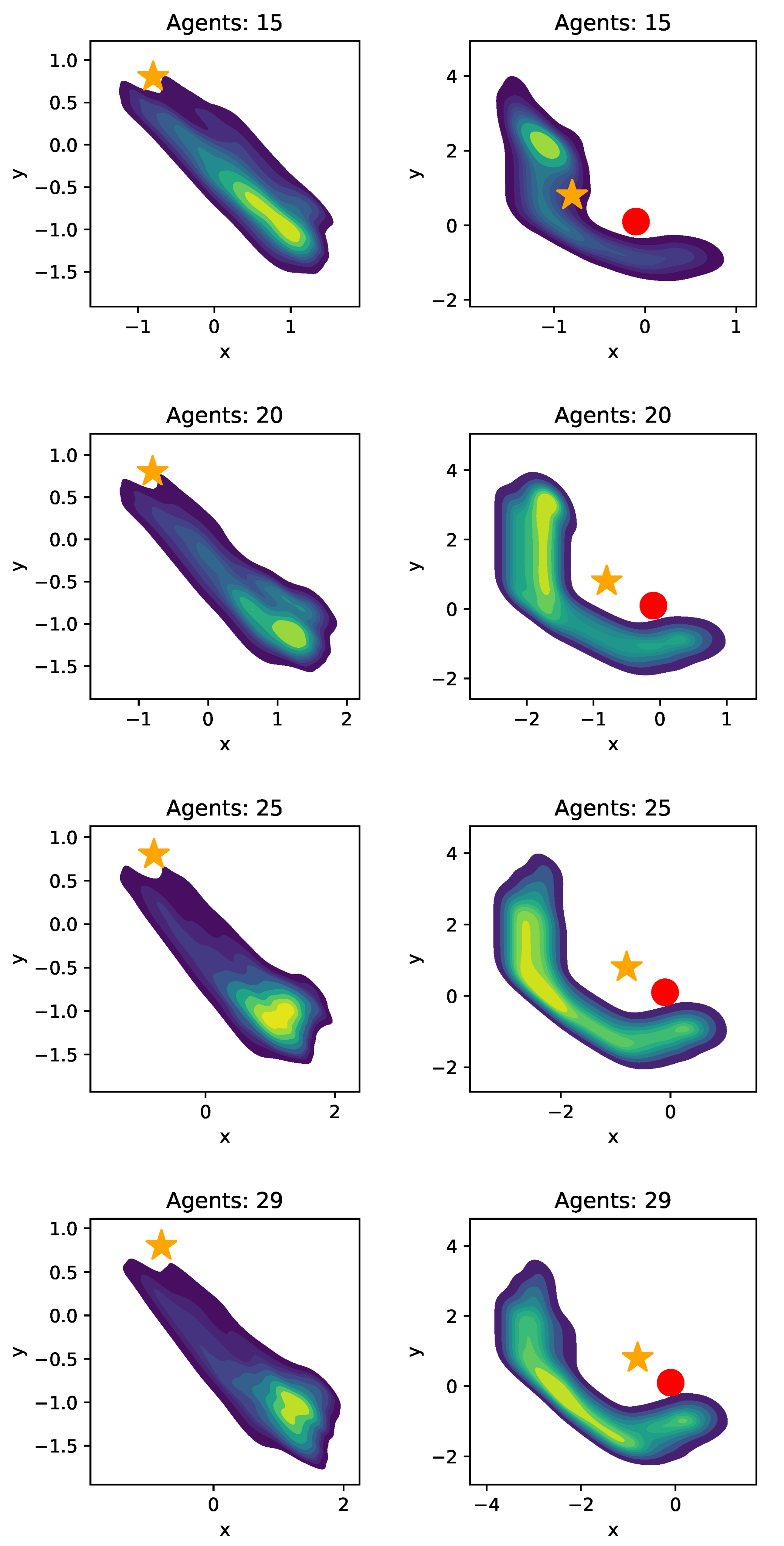
To visualize the agents’ spatial distribution, the kernel density estimation (KDE) plots of the agents’ positions during episodes are presented in Figure 6. For the Go to Position task (top row), formations are more compact at smaller team sizes and become progressively more dispersed as the swarm size increases.
In the Obstacle Avoidance task, the box plots show near-zero collisions across all swarm sizes, indicating successful obstacle avoidance behavior. However, the center panel reveals increasing average distances to the goal as the swarm size grows. The KDE plots for this task (bottom row) demonstrate that as the swarm size increases, the spatial distribution shifts to give progressively wider berth to the obstacle area, suggesting a stronger emphasis on collision avoidance relative to goal-seeking behavior. This is also evident in Figure 7, where agents navigate around the obstacle while moving towards the goal, with larger swarms showing more pronounced avoidance patterns.

6. Discussion

The experimental results reveal important aspects about how GNN-based approaches to swarm coordination handle varying numbers of agents. Our analysis highlights both promising capabilities and notable limitations of the DGQL approach. The following insights delve into the nature of the learned policies’ scalability, examining how and why performance characteristics change as swarm sizes increase beyond training conditions.
Insight 1: GNN-based policies exhibit near zero-shot scalability, enabling functional coordination in swarms larger than the training size without retraining.
Our results show that the swarms did not collapse into complete disarray when the agent count increased. Agents generally maintained goal-oriented behavior and obstacle avoidance capabilities (Figure 5, right panel shows near-zero collisions). This contrasts with many traditional MARL approaches where policies are highly brittle to changes in agent numbers. The GNN’s ability to process variable-sized neighborhood graphs seems key to this basic generalization.
Insight 2: While functional, the efficiency of the learned coordination policy degrades monotonically as the swarm size deviates from the training size.
Despite this near zero-shot scalability, performance gradually degrades as the swarm size diverges from the training configuration. This decline is evident in the steadily increasing average distance to the goal observed in both tasks as agent numbers rise (Figure 5, left and center panels), with no counterexamples in our evaluated sizes. Although the GNN architecture can handle variable neighbor counts, the coordination patterns learned from a ten-agent swarm (e.g., ideal spacing and synchronized movements) do not seamlessly adapt to much larger groups (e.g., 28–30 agents). As agent density and interaction complexity increase, the policy struggles to maintain the same level of efficiency.
Insight 3: The nature of performance degradation under scalability stress is task-dependent, potentially revealing shifts in learned behavioral priorities.
In the simpler Go to Position task, degradation manifested primarily as less efficient convergence and more dispersed formations (Figure 6, top row). However, in the Obstacle Avoidance task, the agents increasingly prioritized avoiding the obstacle over reaching the goal in larger swarms (Figure 6, bottom row), even though goal distance suffered (Figure 5, center panel). This suggests the penalty term for obstacle proximity, effectively learned during training, becomes dominant in the more crowded scenarios encountered at larger scales, leading to overly cautious behavior. The GNN-learned policy seems to adapt its risk assessment based on local density, which changes with swarm size.
Insight 4: Safety-Efficiency Trade-off in Obstacle Avoidance.
The observed tendency of obstacle avoidance policies to prioritize safety over efficiency as swarm size increases can be attributed to both reward shaping and density effects. The reward formulation (Equation (17)) defines a local penalty applied to each agent when it approaches the obstacle. As swarm density increases, a larger fraction of agents are likely to enter the penalty zone at any given time, making these negative rewards more frequent within the collective experience buffer. Consequently, the shared policy becomes biased toward conservative behaviors that maintain greater distances from obstacles, emphasizing safety over speed or path efficiency.
From a scalability perspective, this reflects a self-regulating mechanism emerging from local interactions: as local density rises, the probability of receiving proximity penalties increases, leading to emergent collective caution. While this reduces overall efficiency, it ensures functional safety and coordination even in larger swarms.
Insight 5: The fixed neighborhood definition (k-nearest) and GNN receptive field (K-hop) -might limit scalability by providing an incomplete -or biased view of the relevant coordination state in larger swarms.
The policy relies on information aggregated from a fixed number (five) of nearest neighbors and processed through a shallow GNN (one layer). While sufficient for ten agents, this local view may become inadequate as the swarm grows. Important coordination information might exist beyond the immediate neighbors or the 1-hop GNN range, or the dynamics within the k-nearest neighbors might change significantly in denser configurations. This suggests that the chosen GNN architecture and neighborhood definition, while enabling some scaling, might be a bottleneck for larger jumps in swarm size.
Insight 6: The rate of efficiency loss accelerates once the swarm exceeds roughly twice the training population.
Comparing 15/20 agents to 25/29 agents reveals a steeper rise in terminal distance beyond twice the training size (ten agents). This suggests density-driven interaction effects and receptive-field limitations compound with scale, amplifying inefficiencies in larger swarms even as functional safety (near-zero collisions) is retained.

6.1. Final Remarks

Collectively, these insights sharpen the answer to our research question: GNN-based policies generalize functionally across population changes without retraining, but efficiency degrades as deployment size diverges from training, with task-dependent trade-offs. In our setup, efficiency declines monotonically across the tested sizes (15 to 29 agents) and degrades more rapidly once exceeding twice the training size, suggesting that density and receptive-field mismatches increasingly impact performance as populations grow. Closing this gap likely requires scale-aware training (population/density randomization, curricula, scale-conditioned policies), architectures with adaptive neighborhoods and larger effective receptive fields (deeper/residual attention-based GNNs with degree/density normalization), and objectives that explicitly balance safety and goal progress across scales. These directions aim to preserve zero-shot generalization while stabilizing efficiency; we now turn to limitations and threats to validity.

6.2. Limitations and Threats to Validity

Our study has several limitations that should be considered when interpreting the results, though each represents a deliberate methodological choice with specific justifications as the following:
  • Limited training diversity: We train on a single swarm size (ten agents), which may bias the learned coordination patterns toward this specific scale and limit generalization to significantly different sizes. However, this choice enables a controlled investigation of zero-shot scalability—training on diverse swarm sizes would conflate learning scalable representations with learning to handle size variation directly.
  • Shallow GNN architecture: Our use of single-layer message passing ( K = 1 ) constrains the receptive field to immediate neighbors, potentially missing longer-range coordination dependencies critical for larger swarms. This limitation is deliberate and aligns with minimal local-rule models (e.g., Reynolds’ Boids [61]). The agents react only to 1-hop neighbors via a sparse kNN neighborhood in our case), letting coordination emerge as information propagates over time through motion rather than explicit multi-hop messaging. This choice reduces communication and computation, avoids oversmoothing, and supports real-time deployment.
  • Simplified communication model: The k-nearest neighbor topology may not accurately reflect real-world communication constraints, such as limited bandwidth, interference, or range limitations in physical robot platforms. Nevertheless, the kNN model provides a reasonable approximation of proximity-based communication common in robotic swarms, and the k = 5 parameter choice represents realistic communication fanout for resource-constrained devices.
  • Task complexity: Our evaluation focuses on relatively simple 2D navigation tasks with basic dynamics. More complex scenarios involving heterogeneous objectives, dynamic environments, or 3D coordination may reveal different scalability patterns. We deliberately chose these canonical swarm coordination problems to establish baseline scalability behavior in well-understood scenarios before tackling more complex domains. The tasks capture fundamental swarm coordination challenges (collision avoidance, goal convergence, formation maintenance) that form building blocks for more sophisticated behaviors.
  • Limited evaluation metrics: We primarily assess terminal distance to goal and collision counts, omitting other important factors such as energy consumption, communication overhead, convergence time, and trajectory efficiency that may be critical for real deployments. Our metric selection focuses on task completion quality—the most direct measure of coordination effectiveness—while additional metrics would be valuable for comprehensive deployment evaluation.
  • Hyperparameter sensitivity: We did not perform an explicit sensitivity analysis on the hyperparameters of the proposed method. While this choice keeps the focus on scalability behavior, exploring how parameter variations affect performance represents an important direction for future work.
Despite these limitations, our results provide meaningful evidence for GNN-based scalability in swarm coordination. The methodological choices reflect a research strategy that prioritizes controlled evaluation of specific hypotheses over comprehensive real-world validation, establishing a foundation for future work that can address deployment considerations systematically.

7. Conclusions and Future Work

In this paper, we address the challenge of achieving scalable policy learning for homogeneous swarms of agents. To this end, we formalize Deep graph Q-learning (DGQL), an extension of the standard deep Q-learning algorithm that incorporates Graph Neural Networks (GNNs), therefore exploiting the generalization capabilities inherent to graph-based representations in the context of collective tasks. Our empirical results demonstrate that DGQL can scale policies learned on small agent groups to larger swarms, preserving functional coordination and safety without retraining; however, efficiency declines monotonically with increasing team size across the tested range (15–29 agents), with a steeper degradation once the swarm exceeds twice the training size.
Future work will explore extending our approach to additional benchmark environments, such as those provided by VMAS [58], and examining alternative GNN architectures (e.g., Graph Convolutional Networks [62] or GraphSAGE [63]) to enhance robustness and scalability. Additionally, we plan to extend our approach to heterogeneous swarms comprising agents with diverse sensing or actuation capabilities, to evaluate the generality of the proposed framework beyond the homogeneous setting. Moreover, we plan to investigate the role of GNN depth in this context to determine whether excessive message passing may lead to homogenized representations and reduced performance. These investigations aim to further advance the design of scalable, decentralized control policies for complex multi-agent systems.

Author Contributions

Conceptualization, G.A., D.D. and M.V.; methodology, G.A., D.D. and M.V.; software, G.A., D.D., and F.V.; validation, G.A., D.D. and F.V.; investigation, G.A., D.D. and F.V.; data curation, G.A., D.D. and F.V.; writing—original draft preparation, G.A. and D.D.; writing—review and editing, G.A. and D.D.; visualization, G.A. and D.D.; supervision, M.V.; funding acquisition, M.V. All authors have read and agreed to the published version of the manuscript.

Funding

This work was supported by the FAIR foundation, funded by the European Commission under the NextGenerationEU programme (PNRR, M4C2, Investimento 1.3, Partenariato Esteso PE00000013, Spoke 8 “Pervasive AI”).

Institutional Review Board Statement

Not applicable.

Informed Consent Statement

Not applicable.

Data Availability Statement

The data generated for the evaluation purposes are publicly available at the repository linked in Section 5.

Conflicts of Interest

The authors declare no conflicts of interest.

References

  1. Schranz, M.; Umlauft, M.; Sende, M.; Elmenreich, W. Swarm Robotic Behaviors and Current Applications. Front. Robot. AI 2020, 7, 36. [Google Scholar] [CrossRef]
  2. Tahir, A.; Böling, J.M.; Haghbayan, M.H.; Toivonen, H.T.; Plosila, J. Swarms of Unmanned Aerial Vehicles—A Survey. J. Ind. Inf. Integr. 2019, 16, 100106. [Google Scholar] [CrossRef]
  3. Domini, D.; Farabegoli, N.; Aguzzi, G.; Viroli, M. Towards Intelligent Pulverized Systems: A Modern Approach for Edge-Cloud Services. In Proceedings of the 25th Workshop “From Objects to Agents”, Bard, Italy, 8–10 July 2024; Volume 3735, pp. 233–251. [Google Scholar]
  4. Orr, J.; Dutta, A. Multi-Agent Deep Reinforcement Learning for Multi-Robot Applications: A Survey. Sensors 2023, 23, 3625. [Google Scholar] [CrossRef]
  5. Sosic, A.; KhudaBukhsh, W.R.; Zoubir, A.M.; Koeppl, H. Inverse Reinforcement Learning in Swarm Systems. In Proceedings of the 16th Conference on Autonomous Agents and MultiAgent Systems, AAMAS 2017, São Paulo, Brazil, 8–12 May 2017; Larson, K., Winikoff, M., Das, S., Durfee, E.H., Eds.; ACM: New York, NY, USA, 2017; pp. 1413–1421. [Google Scholar]
  6. Domini, D.; Aguzzi, G.; Pianini, D.; Viroli, M. A Reusable Simulation Pipeline for Many-Agent Reinforcement Learning. In Proceedings of the 28th IEEE/ACM International Symposium on Distributed Simulation and Real Time Applications, DS-RT 2024, Urbino, Italy, 5–9 October 2024; IEEE: Piscataway, NJ, USA, 2024. [Google Scholar]
  7. Malucelli, N.; Domini, D.; Aguzzi, G.; Viroli, M. Neighbor-Based Decentralized Training Strategies for Multi-Agent Reinforcement Learning. In Proceedings of the 40th ACM/SIGAPP Symposium on Applied Computing, SAC 2025, Catania, Italy, 31 March–4 April 2025; ACM: New York, NY, USA, 2024; pp. 3–10. [Google Scholar] [CrossRef]
  8. Yang, Y.; Luo, R.; Li, M.; Zhou, M.; Zhang, W.; Wang, J. Mean Field Multi-Agent Reinforcement Learning. In Proceedings of the 35th International Conference on Machine Learning, ICML 2018, Stockholmsmässan, Stockholm, Sweden, 10–15 July 2018; Volume 80, pp. 5567–5576. [Google Scholar]
  9. Domini, D.; Cavallari, F.; Aguzzi, G.; Viroli, M. ScaRLib: Towards a hybrid toolchain for aggregate computing and many-agent reinforcement learning. Sci. Comput. Program. 2024, 238, 103176. [Google Scholar] [CrossRef]
  10. Wu, Z.; Pan, S.; Chen, F.; Long, G.; Zhang, C.; Yu, P.S. A Comprehensive Survey on Graph Neural Networks. IEEE Trans. Neural Networks Learn. Syst. 2021, 32, 4–24. [Google Scholar] [CrossRef] [PubMed]
  11. Aguzzi, G.; Viroli, M.; Esterle, L. Field-informed Reinforcement Learning of Collective Tasks with Graph Neural Networks. In Proceedings of the IEEE International Conference on Autonomic Computing and Self-Organizing Systems, ACSOS 2023, Toronto, ON, Canada, 25–29 September 2023; IEEE: Piscataway, NJ, USA, 2023; pp. 37–46. [Google Scholar] [CrossRef]
  12. Busoniu, L.; Babuska, R.; De Schutter, B. A Comprehensive Survey of Multiagent Reinforcement Learning. IEEE Trans. Syst. Man Cybern. Part C Appl. Rev. 2008, 38, 156–172. [Google Scholar] [CrossRef]
  13. Tan, M. Multi-agent reinforcement learning: Independent versus cooperative agents. In Proceedings of the Tenth International Conference on International Conference on Machine Learning, ICML’93, San Francisco, CA, USA, 27–29 July 1993; pp. 330–337. [Google Scholar]
  14. Wang, X.; Ke, L.; Zhang, G.; Zhu, D. Adaptive mean field multi-agent reinforcement learning. Inf. Sci. 2024, 669, 120560. [Google Scholar] [CrossRef]
  15. Mondal, W.U.; Agarwal, M.; Aggarwal, V.; Ukkusuri, S.V. On the approximation of cooperative heterogeneous multi-agent reinforcement learning (MARL) using Mean Field Control (MFC). J. Mach. Learn. Res. 2022, 23, 1–46. [Google Scholar]
  16. Li, C.; Wang, T.; Wu, C.; Zhao, Q.; Yang, J.; Zhang, C. Celebrating Diversity in Shared Multi-Agent Reinforcement Learning. In Proceedings of the Advances in Neural Information Processing Systems 34: Annual Conference on Neural Information Processing Systems 2021, NeurIPS 2021, Virtual, 6–14 December 2021; pp. 3991–4002. [Google Scholar]
  17. Nayak, S.; Choi, K.; Ding, W.; Dolan, S.; Gopalakrishnan, K.; Balakrishnan, H. Scalable Multi-Agent Reinforcement Learning through Intelligent Information Aggregation. In Proceedings of the International Conference on Machine Learning, ICML 2023, Honolulu, HI, USA, 23–29 July 2023; Volume 202, pp. 25817–25833. [Google Scholar]
  18. Lin, Y.; Wan, Z.; Yang, Z. HGAP: Boosting permutation invariant and permutation equivariant multi-agent reinforcement learning with graph attention. In Proceedings of the 41st International Conference on Machine Learning (ICML 2024). PMLR, Vienna, Austria, 21–27 July 2024; pp. 30615–30648. [Google Scholar]
  19. Mahjoub, O.; Abramowitz, S.; de Kock, R.; Khlifi, W.; du Toit, S.; Daniel, J.; Nessir, L.B.; Beyers, L.; Formanek, C.; Clark, L.; et al. Performant, Memory Efficient and Scalable Multi-Agent Reinforcement Learning. arXiv 2024, arXiv:2410.01706. [Google Scholar] [CrossRef]
  20. Jiang, J.; Dun, C.; Huang, T.; Lu, Z. Graph Convolutional Reinforcement Learning. In Proceedings of the 8th International Conference on Learning Representations, ICLR 2020, Addis Ababa, Ethiopia, 26–30 April 2020. [Google Scholar]
  21. Khan, A.; Ribeiro, A.; Kumar, V.; Jadbabaie, A. Graph policy gradients for large scale robot control. In Proceedings of the Conference on Robot Learning (CoRL 2019), PMLR, Osaka, Japan, 30 October 30–1 November 2019; pp. 823–834. [Google Scholar]
  22. Zhou, M.; Liu, Z.; Sui, P.; Li, Y.; Chung, Y.Y. Learning implicit credit assignment for cooperative multi-agent reinforcement learning. In Proceedings of the Advances in Neural Information Processing Systems (NeurIPS 2020), Virtual, 6–12 December 2020; Volume 33, pp. 11853–11864. [Google Scholar]
  23. Lowe, R.; Wu, Y.I.; Tamar, A.; Harb, J.; Abbeel, P.; Mordatch, I. Multi-agent actor-critic for mixed cooperative-competitive environments. In Proceedings of the Advances in Neural Information Processing Systems (NeurIPS 2017), Long Beach, CA, USA, 4–9 December 2017; Volume 30. [Google Scholar]
  24. Sunehag, P.; Lever, G.; Gruslys, A.; Czarnecki, W.M.; Zambaldi, V.; Jaderberg, M.; Lanctot, M.; Sonnerat, N.; Leibo, J.Z.; Tuyls, K.; et al. Value-decomposition networks for cooperative multi-agent learning. arXiv 2017, arXiv:1706.05296. [Google Scholar]
  25. Rashid, T.; Samvelyan, M.; de Witt, C.S.; Farquhar, G.; Foerster, J.N.; Whiteson, S. QMIX: Monotonic Value Function Factorisation for Deep Multi-Agent Reinforcement Learning. In Proceedings of the 35th International Conference on Machine Learning, ICML 2018, Stockholmsmässan, Stockholm, Sweden, 10–15 July 2018; Volume 80, pp. 4292–4301. [Google Scholar]
  26. Son, K.; Kim, D.; Kang, W.J.; Hostallero, D.; Yi, Y. QTRAN: Learning to Factorize with Transformation for Cooperative Multi-Agent Reinforcement Learning. In Proceedings of the 36th International Conference on Machine Learning, ICML 2019, Long Beach, CA, USA, 9–15 June 2019; Volume 97, pp. 5887–5896. [Google Scholar]
  27. Wang, J.; Ren, Z.; Liu, T.; Yu, Y.; Zhang, C. QPLEX: Duplex Dueling Multi-Agent Q-Learning. In Proceedings of the 9th International Conference on Learning Representations, ICLR 2021, Virtual Event, 3–7 May 2021. [Google Scholar]
  28. Baisero, A.; Bhati, R.; Liu, S.; Pillai, A.; Amato, C. Fixing Incomplete Value Function Decomposition for Multi-Agent Reinforcement Learning. arXiv 2025. [Google Scholar] [CrossRef]
  29. Foerster, J.N.; Farquhar, G.; Afouras, T.; Nardelli, N.; Whiteson, S. Counterfactual Multi-Agent Policy Gradients. In Proceedings of the Thirty-Second AAAI Conference on Artificial Intelligence, (AAAI-18), the 30th Innovative Applications of Artificial Intelligence (IAAI-18), and the 8th AAAI Symposium on Educational Advances in Artificial Intelligence (EAAI-18), New Orleans, LA, USA, 2–7 February 2018; McIlraith, S.A., Weinberger, K.Q., Eds.; AAAI Press: Menlo Park, CA, USA, 2018; pp. 2974–2982. [Google Scholar] [CrossRef]
  30. Zhang, K.; Yang, Z.; Basar, T. Multi-Agent Reinforcement Learning: A Selective Overview of Theories and Algorithms. arXiv 2019, arXiv:1911.10635. [Google Scholar]
  31. Li, Y.; Wang, L.; Yang, J.; Wang, E.; Wang, Z.; Zhao, T.; Zha, H. Permutation Invariant Policy Optimization for Mean-Field Multi-Agent Reinforcement Learning: A Principled Approach. arXiv 2021, arXiv:2105.08268. [Google Scholar]
  32. Hao, J.; Hao, X.; Mao, H.; Wang, W.; Yang, Y.; Li, D.; Zheng, Y.; Wang, Z. Boosting Multiagent Reinforcement Learning via Permutation Invariant and Permutation Equivariant Networks. In Proceedings of the The Eleventh International Conference on Learning Representations, ICLR 2023, Kigali, Rwanda, 1–5 May 2023. [Google Scholar]
  33. Amato, C. An Introduction to Centralized Training for Decentralized Execution in Cooperative Multi-Agent Reinforcement Learning. arXiv 2024, arXiv:2409.03052. [Google Scholar] [CrossRef]
  34. Zhou, Y.; Liu, S.; Qing, Y.; Chen, K.; Zheng, T.; Huang, Y.; Song, J.; Song, M. Is Centralized Training with Decentralized Execution Framework Centralized Enough for MARL? arXiv 2023, arXiv:2305.17352. [Google Scholar] [CrossRef]
  35. Sukhbaatar, S.; Szlam, A.; Fergus, R. Learning Multiagent Communication with Backpropagation. In Proceedings of the Advances in Neural Information Processing Systems 29: Annual Conference on Neural Information Processing Systems 2016, Barcelona, Spain, 5–10 December 2016; pp. 2244–2252. [Google Scholar]
  36. Das, A.; Gervet, T.; Romoff, J.; Batra, D.; Parikh, D.; Rabbat, M.; Pineau, J. TarMAC: Targeted Multi-Agent Communication. In Proceedings of the 36th International Conference on Machine Learning, ICML 2019, Long Beach, CA, USA, 9–15 June 2019; Volume 97, pp. 1538–1546. [Google Scholar]
  37. Singh, A.; Jain, T.; Sukhbaatar, S. Learning when to Communicate at Scale in Multiagent Cooperative and Competitive Tasks. In Proceedings of the 7th International Conference on Learning Representations, ICLR 2019, New Orleans, LA, USA, 6–9 May 2019. [Google Scholar]
  38. Hu, D.; Zhang, C.; Prasanna, V.K.; Krishnamachari, B. Learning Practical Communication Strategies in Cooperative Multi-Agent Reinforcement Learning. In Proceedings of the Asian Conference on Machine Learning, ACML 2022, Hyderabad, India, 12–14 December 2022; Volume 189, pp. 467–482. [Google Scholar]
  39. Shao, J.; Zhang, H.; Qu, Y.; Liu, C.; He, S.; Jiang, Y.; Ji, X. Complementary Attention for Multi-Agent Reinforcement Learning. In Proceedings of the International Conference on Machine Learning, ICML 2023, Honolulu, HI, USA, 23–29 July 2023; Volume 202, pp. 30776–30793. [Google Scholar]
  40. Guo, X.; Shi, D.; Fan, W. Scalable Communication for Multi-Agent Reinforcement Learning via Transformer-Based Email Mechanism. In Proceedings of the Thirty-Second International Joint Conference on Artificial Intelligence, IJCAI 2023, Macao, SAR, China, 19–25 August 2023; pp. 126–134. [Google Scholar] [CrossRef]
  41. Liu, Z.; Zhang, J.; Shi, E.; Liu, Z.; Niyato, D.; Ai, B.; Shen, X. Graph Neural Network Meets Multi-Agent Reinforcement Learning: Fundamentals, Applications, and Future Directions. Wireless Commun. 2024, 31, 39–47. [Google Scholar] [CrossRef]
  42. Du, H.; Gou, F.; Cai, Y. Scalable Safe Multi-Agent Reinforcement Learning for Multi-Agent System. arXiv 2025, arXiv:2501.13727. [Google Scholar] [CrossRef]
  43. Baldazo, D.; Parras, J.; Zazo, S. Decentralized Multi-Agent Deep Reinforcement Learning in Swarms of Drones for Flood Monitoring. In Proceedings of the 27th European Signal Processing Conference, EUSIPCO 2019, A Coruña, Spain, 2–6 September 2019; IEEE: Piscataway, NJ, USA, 2019; pp. 1–5. [Google Scholar] [CrossRef]
  44. Silver, D.; Hubert, T.; Schrittwieser, J.; Antonoglou, I.; Lai, M.; Guez, A.; Lanctot, M.; Sifre, L.; Kumaran, D.; Graepel, T.; et al. Mastering Chess and Shogi by Self-Play with a General Reinforcement Learning Algorithm. arXiv 2017, arXiv:1712.01815. [Google Scholar] [CrossRef]
  45. Silver, D.; Huang, A.; Maddison, C.J.; Guez, A.; Sifre, L.; van den Driessche, G.; Schrittwieser, J.; Antonoglou, I.; Panneershelvam, V.; Lanctot, M.; et al. Mastering the game of Go with deep neural networks and tree search. Nature 2016, 529, 484–489. [Google Scholar] [CrossRef]
  46. Vinyals, O.; Babuschkin, I.; Czarnecki, W.M.; Mathieu, M.; Dudzik, A.; Chung, J.; Choi, D.H.; Powell, R.; Ewalds, T.; Georgiev, P.; et al. Grandmaster level in StarCraft II using multi-agent reinforcement learning. Nature 2019, 575, 350–354. [Google Scholar] [CrossRef]
  47. Berner, C.; Brockman, G.; Chan, B.; Cheung, V.; Debiak, P.; Dennison, C.; Farhi, D.; Fischer, Q.; Hashme, S.; Hesse, C.; et al. Dota 2 with Large Scale Deep Reinforcement Learning. arXiv 2019, arXiv:1912.06680. [Google Scholar] [CrossRef]
  48. Andrychowicz, M.; Baker, B.; Chociej, M.; Józefowicz, R.; McGrew, B.; Pachocki, J.; Petron, A.; Plappert, M.; Powell, G.; Ray, A.; et al. Learning dexterous in-hand manipulation. Int. J. Robot. Res. 2020, 39, 3–20. [Google Scholar] [CrossRef]
  49. OpenAI; Akkaya, I.; Andrychowicz, M.; Chociej, M.; Litwin, M.; McGrew, B.; Petron, A.; Paino, A.; Plappert, M.; Powell, G.; et al. Solving Rubik’s Cube with a Robot Hand. arXiv 2019, arXiv:1910.07113. [Google Scholar]
  50. Watkins, C.J.; Dayan, P. Q-learning. Mach. Learn. 1992, 8, 279–292. [Google Scholar] [CrossRef]
  51. Mnih, V.; Kavukcuoglu, K.; Silver, D.; Rusu, A.A.; Veness, J.; Bellemare, M.G.; Graves, A.; Riedmiller, M.A.; Fidjeland, A.; Ostrovski, G.; et al. Human-level control through deep reinforcement learning. Nature 2015, 518, 529–533. [Google Scholar] [CrossRef]
  52. Chen, G. A New Framework for Multi-Agent Reinforcement Learning—Centralized Training and Exploration with Decentralized Execution via Policy Distillation. In Proceedings of the 19th International Conference on Autonomous Agents and Multiagent Systems, AAMAS ’20, Auckland, New Zealand, 9–13 May 2020; Seghrouchni, A.E.F., Sukthankar, G., An, B., Yorke-Smith, N., Eds.; International Foundation for Autonomous Agents and Multiagent Systems: Istanbul, Turkey, 2020; pp. 1801–1803. [Google Scholar]
  53. Azzam, R.; Boiko, I.; Zweiri, Y. Swarm Cooperative Navigation Using Centralized Training and Decentralized Execution. Drones 2023, 7, 193. [Google Scholar] [CrossRef]
  54. Gilmer, J.; Schoenholz, S.S.; Riley, P.F.; Vinyals, O.; Dahl, G.E. Neural Message Passing for Quantum Chemistry. In Proceedings of the 34th International Conference on Machine Learning, ICML 2017, Sydney, NSW, Australia, 6–11 August 2017; Volume 70, pp. 1263–1272. [Google Scholar]
  55. Brambilla, M.; Ferrante, E.; Birattari, M.; Dorigo, M. Swarm robotics: A review from the swarm engineering perspective. Swarm Intell. 2013, 7, 1–41. [Google Scholar] [CrossRef]
  56. Bayindir, L. A review of swarm robotics tasks. Neurocomputing 2016, 172, 292–321. [Google Scholar] [CrossRef]
  57. Domini, D.; Cavallari, F.; Aguzzi, G.; Viroli, M. ScaRLib: A Framework for Cooperative Many Agent Deep Reinforcement Learning in Scala. In Proceedings of the Coordination Models and Languages—25th IFIP WG 6.1 International Conference, COORDINATION 2023, Held as Part of the 18th International Federated Conference on Distributed Computing Techniques, DisCoTec 2023, Lisbon, Portugal, 18–23 June 2023; Proceedings. Jongmans, S., Lopes, A., Eds.; Springer: Berlin/Heidelberg, Germany, 2023; Volume 13908, pp. 52–70. [Google Scholar] [CrossRef]
  58. Bettini, M.; Kortvelesy, R.; Blumenkamp, J.; Prorok, A. VMAS: A Vectorized Multi-agent Simulator for Collective Robot Learning. In Proceedings of the Distributed Autonomous Robotic Systems—16th International Symposium, DARS 2022, Montbéliard, France, 28–30 November 2022; Bourgeois, J., Paik, J., Piranda, B., Werfel, J., Hauert, S., Pierson, A., Hamann, H., Lam, T.L., Matsuno, F., Mehr, N., et al., Eds.; Springer: Berlin/Heidelberg, Germany, 2022; Volume 28, pp. 42–56. [Google Scholar] [CrossRef]
  59. Paszke, A.; Gross, S.; Chintala, S.; Chanan, G.; Yang, E.; DeVito, Z.; Lin, Z.; Desmaison, A.; Antiga, L.; Lerer, A. Automatic Differentiation in Pytorch. In Proceedings of the 31st Conference on Neural Information Processing Systems (NIPS 2017), Long Beach, CA, USA, 4–9 December 2017. [Google Scholar]
  60. Fey, M.; Lenssen, J.E. Fast Graph Representation Learning with PyTorch Geometric. arXiv 2019, arXiv:1903.02428. [Google Scholar] [CrossRef]
  61. Reynolds, C.W. Flocks, herds and schools: A distributed behavioral model. In Proceedings of the 14th Annual Conference on Computer Graphics and Interactive Techniques, SIGGRAPH 1987, Anaheim, CA, USA, 27–31 July 1987; Stone, M.C., Ed.; ACM: New York, NY, USA, 1987; pp. 25–34. [Google Scholar] [CrossRef]
  62. Kipf, T.N.; Welling, M. Semi-Supervised Classification with Graph Convolutional Networks. In Proceedings of the 5th International Conference on Learning Representations, ICLR 2017, Toulon, France, 24–26 April 2017. [Google Scholar]
  63. Hamilton, W.L.; Ying, Z.; Leskovec, J. Inductive Representation Learning on Large Graphs. In Proceedings of the Advances in Neural Information Processing Systems 30: Annual Conference on Neural Information Processing Systems 2017, Long Beach, CA, USA, 4–9 December 2017; pp. 1024–1034. [Google Scholar]
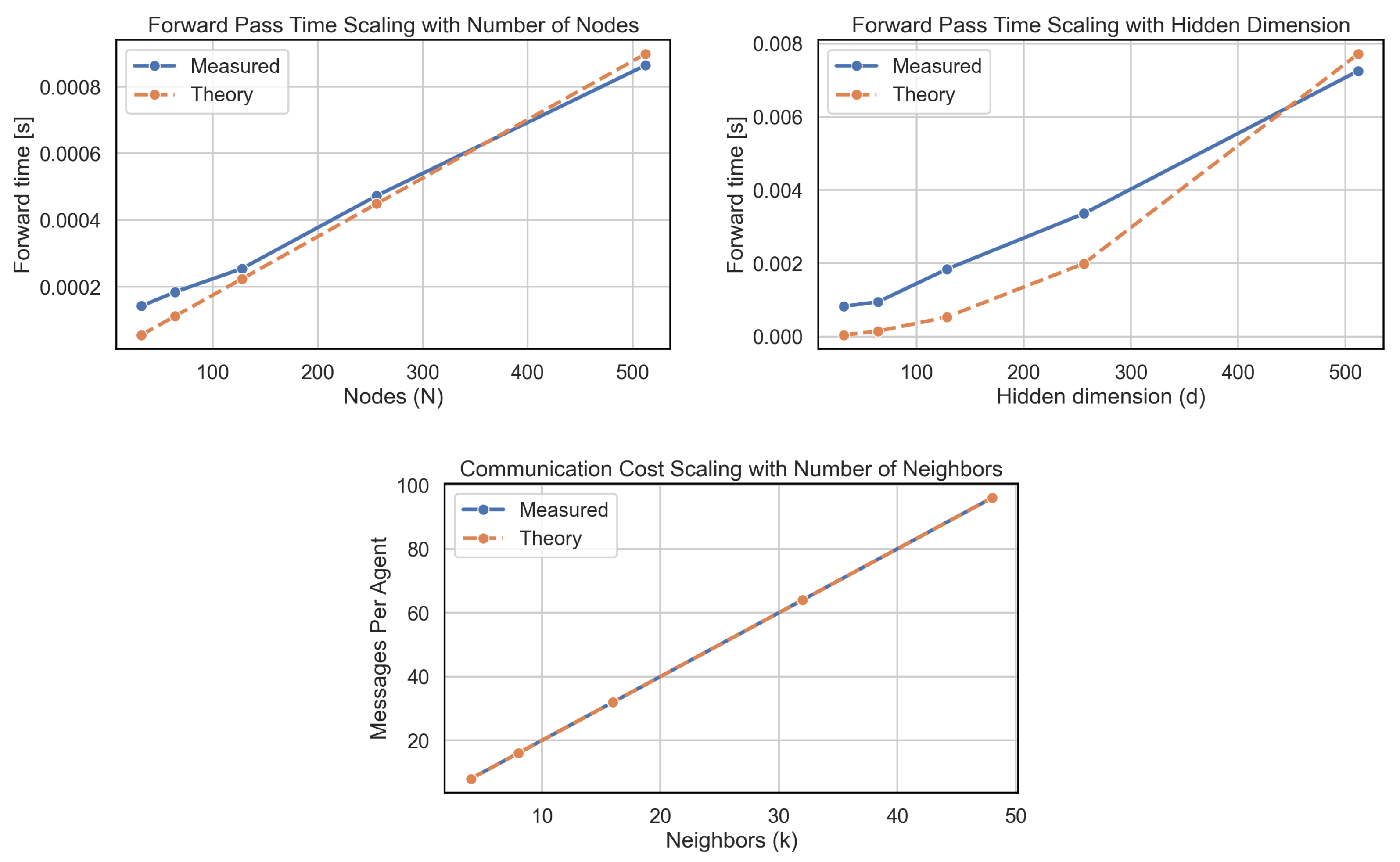
Figure 1. Empirical and theoretical scaling of GNN inference cost. Forward pass time scales linearly with the number of nodes and quadratically with the hidden dimension, while communication cost grows linearly with the neighborhood size k.
Ai 06 00282 g001
Figure 2. The Go to Position task. The agents (green dots) must converge to a target location (black dot).
Ai 06 00282 g002
Figure 4. Training results for the Go to Position (top) and Obstacle Avoidance (bottom) tasks, averaged over four seeds. The left column shows the loss, while the right column the cumulative reward over episodes. Both tasks exhibit decreasing loss and increasing reward, though the Obstacle Avoidance task is noisier.
Ai 06 00282 g004
Figure 5. Testing results for the Go to Position (left) and Obstacle Avoidance (right) tasks with varying swarm sizes. The box plots show the average terminal distance and number of collisions across runs. For Go to Position, performance degrades beyond roughly twice the training size, while Obstacle Avoidance remains mostly collision-free but with increasing terminal distance.
Ai 06 00282 g005
Figure 6. The kernel density estimation (KDE) plots showing agent position distributions for the Go to Position (left column) and Obstacle Avoidance (right column) tasks with increasing swarm sizes (15, 20, 25, 29 agents, top to bottom).
Ai 06 00282 g006
Figure 7. Trajectories of agents in the Obstacle Avoidance task for different swarm sizes (15, 20, 26, and 29 agents) in one episode. Each color represents a different agent, the star indicates the goal and the red cross the obstacle.
Ai 06 00282 g007
Table 2. Simulation parameters.
Simulation Parameters
Environment
Environment size 2 × 2 m
Goal position (training) ( 0.8 , 0.8 )
Initial agent regionnear ( 1.5 , 1.5 )
Episode length (max)100 steps
Training episodes1000
Agents (training)10
Neighborhoodk-NN ( k = 5 )
Position noise N ( 0.6 , 0 . 4 2 )
Obstacle center ( 0.1 , 0.1 )
Obstacle radius 0.2 m
Action Space9 discrete translations
Model
GNN layer (GAT)32 hidden units
Dropout0.1
MLP head2 layers, 32 units
Training
OptimizerAdam ( lr = 10 3 )
Replay buffer 10 6
Batch size32
Discount γ 0.99
Target updateevery 200 steps
Exploration ε exp. decay 1 0.01
Decay rate λ 10 3
Disclaimer/Publisher’s Note: The statements, opinions and data contained in all publications are solely those of the individual author(s) and contributor(s) and not of MDPI and/or the editor(s). MDPI and/or the editor(s) disclaim responsibility for any injury to people or property resulting from any ideas, methods, instructions or products referred to in the content.