From Initialization to Convergence: A Three-Stage Technique for Robust RBF Network Training

Abstract

A parametric machine learning tool with many applications is the radial basis function (RBF) network, which has been incorporated into various classification and regression problems. A key component of these networks is their radial functions. These networks acquire adaptive capabilities through a technique that consists of two stages. The centers and variances are computed in the first stage, and in the second stage, which involves solving a linear system of equations, the external weights for the radial functions are adjusted. Nevertheless, in numerous instances, this training approach has led to decreased performance, either because of instability in arithmetic computations or due to the method’s difficulty in escaping local minima of the error function. In this manuscript, a three-stage method is suggested to address the above problems. In the first phase, an initial estimation of the value ranges for the machine learning model parameters is performed. During the second phase, the network parameters are fine-tuned within the intervals determined in the first phase. Finally, in the third phase of the proposed method, a local optimization technique is applied to achieve the final adjustment of the network parameters. The proposed method was evaluated on several machine learning models from the related literature, as well as compared with the original RBF training approach. This methodhas been successfully applied to a wide range of related problems reported in recent studies. Also, a comparison was made in terms of classification and regression error. It should be noted that although the proposed methodology had very good results in the above measurements, it requires significant computational execution time due to the use of three phases of processing and adaptation of the network parameters.

1. Introduction

Many practical problems can be handled by machine learning tools. Among these problems one can find problems from scientific fields, such as physics [1,2], astronomy [3,4], chemistry [5,6], medicine [7,8], economics [9,10], image processing [11], time series forecasting [12], etc. Among the most widely used machine learning techniques, the radial basis function (RBF) network stands out. A wide range of problems from the real world can be tackled using RBF networks, such as face recognition [13], numerical problems [14,15], economic problems [16], robotics [17,18], network security [19,20], classification of process faults [21], time series prediction [22], estimation of wind power production [23], etc. Moreover, Park et al. [24] proved that an RBF network with one processing layer can approximate any given function.

This paper proposes a three-stage approach for the effective training of RBF networks. The first stage of the method involves an algorithm designed to efficiently determine the value ranges of the model parameters. This detection is implemented using the K-means algorithm [25] for the weights and the variances of the radial functions. After applying the above procedure, a range of values for the network parameters is created that directly depends on the values produced by K-means algorithm. During the second stage of the proposed work, a global optimization procedure is incorporated to optimize the parameters of the RBF network with respect to the training error of the model. The training of the network parameters is performed within the value range of the first phase to avoid possible overfitting problems. In the current work, the genetic algorithm is used as the method of the second phase, but any optimization technique can be incorporated. In the final phase of the proposed method, a local minimization technique is applied to the optimal parameters obtained from the second phase. The aim of the proposed method is first to determine a reliable range of values for the parameters of RBF networks and then to train the network parameters within this range, thereby avoiding potential arithmetic instability issues associated with the conventional RBF training approach.

The proposed technique is the application of three distinct procedures in series, where in each stage the results of the previous phase are used. In the first phase, an initial estimation of the centers and variances is performed with the K-means method. This method is preferred because it is extremely fast to execute and can provide an overview of the search space for neural networks. It is preferred over using random values as this would require a significantly large number of iterations for proper initialization of the parameters. After applying the K-means technique, a range of network parameter values is generated, consisting of multiples of the values obtained from the K-means results. In this way, on the one hand, the use of the K-means technique is utilized and, on the other hand, the second-phase optimization algorithm is given the opportunity to search for parameter values that yield lower values of the error function close to the initial values of the first phase. A genetic algorithm is used as the optimization algorithm in the second phase due to its adaptability to any environment and its widespread use in many computational problems. However, any universal optimization technique could be utilized in this phase. However, although genetic algorithms are extremely effective methods of global optimization, they often do not exactly locate a true minimum of the objective function and therefore the help of a local minimization method is deemed necessary. This occurs in the third phase, where a local optimization method is applied to the chromosome with the smallest value produced in the second phase. The minimum identified in this phase also represents the final outcome of the algorithm, corresponding to a specific configuration of the RBF network parameters.

The main features of the proposed method are its use of multiple techniques in sequence to determine the optimal set of parameters for the machine learning model while avoiding potential overfitting. In the first discrete phase, a well-established clustering method, such as K-means, is employed to identify a promising range of values for the model parameters. In the second phase, a global optimization algorithm is applied to minimize the error function within the bounds established in the first phase. Finally, in the last phase, a local minimization method is used to locate a guaranteed local minimum of the error function. This final phase ensures that the network parameters are trained within the value range determined in the first phase.

The rest of this paper has the following structure: in Section 2, the definition of the RBF networks is presented, as well as some references to related work in the area of training of RBF networks; in Section 3, the parts of the proposed technique are presented in detail; in Section 4, the datasets on which the method was applied are presented, as well as the experimental results from its application; and in Section 5, an extensive discussion of the practical results of the proposed technique is conducted and possible weaknesses that arose during the execution of the experiments are analyzed.

2. Related Work

Typically, any RBF network can be defined through the following equation:

$$R\left(\overrightarrow{x}\right)=\sum _{i=1}^k{w}_i\varphi \left(∥\overrightarrow{x}-\overrightarrow{c_i}∥\right)$$

(1)

The symbols that appear in this equation are defined as follows:

• The input patterns to the model are represented by the vector $\overrightarrow{x}$. The dimension of each pattern is denoted by d.
• The number k denotes the number of weights of the model and the vector $\overrightarrow{w}$ denotes these weights.
• The vectors $\overrightarrow{c_i},i=1,\dots ,k$ denote the centers for the functions used in the network.
• The function $\varphi \left(x\right)$ denotes a Gaussian function defined as follows:

$$\varphi \left(x\right)=\exp \left(-{\displaystyle \frac{{\left(x-c\right)}^2}{{\sigma }^2}}\right)$$

(2)

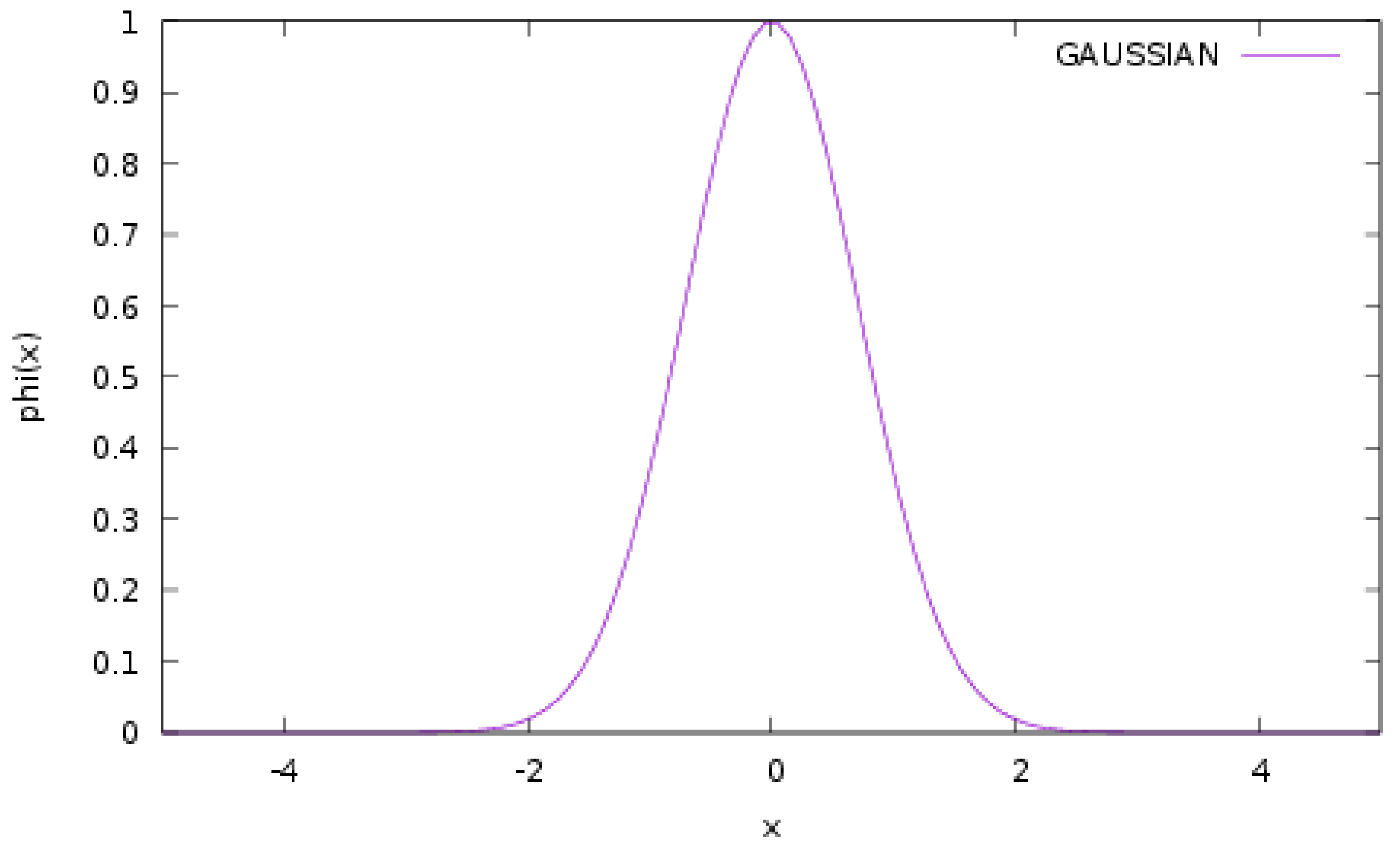
An example plot of the Gaussian function with the parameter set $c=0,\sigma =1$ is shown in Figure 1.

From the graph above, one can conclude that the value of the function rapidly approaches zero as the value of the variable x moves away from the center c. The training error of any given $R\left(x\right)$ RBF network is as follows:

$$E\left(R\left(\overrightarrow{x}\right)\right)=\sum _{i=1}^M{\left(R\left(\overrightarrow{x_i}\right)-y_i\right)}^2$$

(3)

The set $\left(\overrightarrow{x_i},y_i\right),i=1,\dots ,M$ denotes the training set of the objective problem and the values $y_i$ are considered as the actual output for each pattern $\overrightarrow{x_i}$.

Over the past years, numerous techniques have been proposed for training neural networks and efficiently adapting their parameters. Among these, there are methods specifically designed for the effective initialization of RBF network parameters [26,27,28]. Moreover, Benoudjit et al. discussed the estimation of kernels in these models [29]. Additionally, a series of pruning techniques [30,31,32] have been introduced, aiming to reduce the required number of parameters for networks, providing a solution to the overfitting problem. Also, methods that construct the architecture of RBF networks have been proposed recently, such as the work of Du et al. [33] or the work of Yu et al., who suggested an incremental design framework for RBF networks [34]. Also, a series of optimization techniques have been used in the past for the minimization of equation 3, such as genetic algorithms [35], the Particle Swarm Optimization method [36], the Differential Evolution technique [37], etc. Moreover, the rapid growth in the use of parallel computing techniques in recent decades has led to the publication of numerous scientific studies that leverage these methods [38,39]. Recently, Rani et al. proposed an improved PSO optimizer that integrates a differential search mechanism for efficient RBF network training [40]. Moreover, Karamichailidou et al. suggested a novel method for RBF training using variable projection and fuzzy means [41].

In most cases, the above techniques are either limited to local minima of the network error function or fail to adequately classify the problem data due to poor initialization of the network parameters. Furthermore, the above techniques do not specify a range of values for the network parameters within which the optimization of the model parameters can be effectively performed.

3. Materials and Methods

The three distinct phases of the proposed method are discussed here. The discussion initiates with the first phase, where the construction of the ranges for the parameter values is performed using the K-means algorithm. Afterward, the steps of the used genetic algorithm are presented in detail, and finally, this section concludes with the description of the final phase, where a local optimization method is applied to the best-located chromosome of the second phase. Also, the description of the used datasets is provided in this section in table format.

3.1. The Description of the First Phase

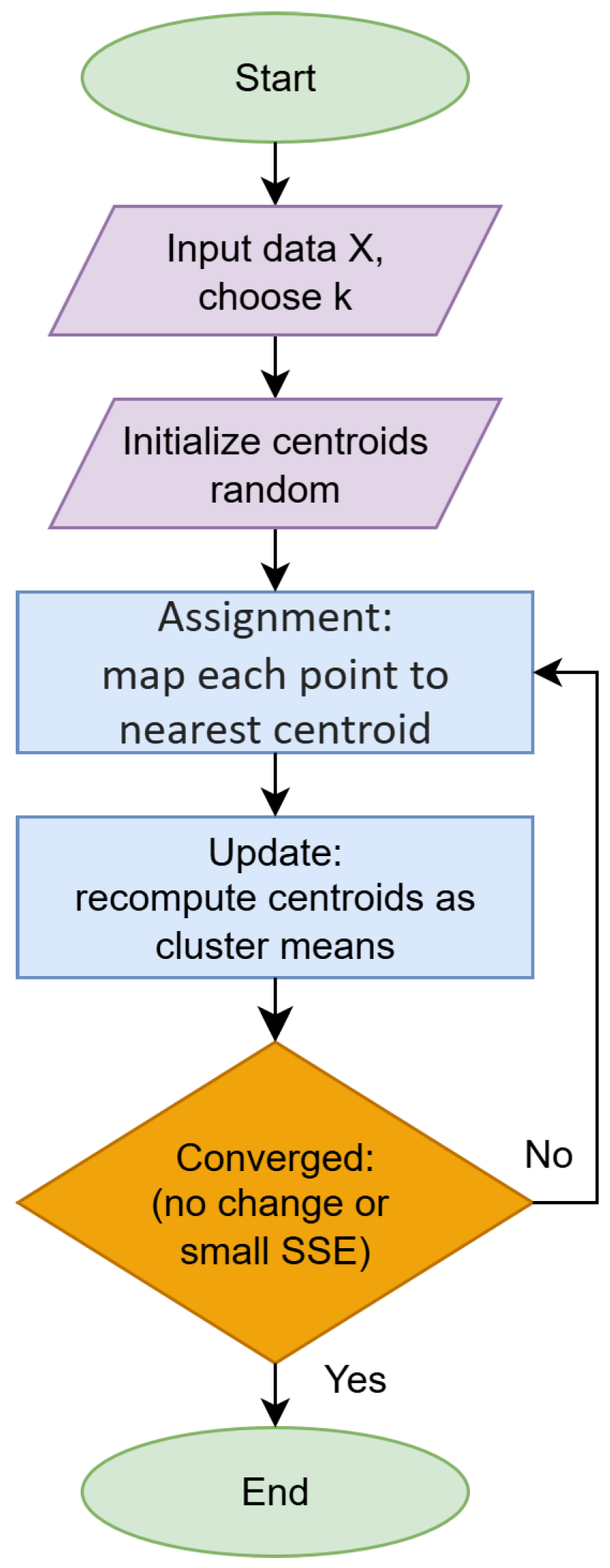
The K-means method, used widely in machine learning, is incorporated in the first phase for the location of the ranges for the centers and variances of the model. This method is incorporated to locate the centers and the variances of the possible groups of a series of points. Furthermore, a series of extensions of this method have been published during the past years, such as the Genetic K-means algorithm [42], the unsupervised K-means algorithm [43], the Fixed-centered K-means algorithm [44], etc. A detailed review of the K-means method can be located in the paper published by Oti et al. [45]. The K-means method is presented in Algorithm 1 A graphical representation is provided in Figure 2.

After the calculation of $\overrightarrow{c_i},i=1,\dots ,k$ and the quantities ${\sigma }_i,i=1,\dots ,k$, the method locates the margin vectors $\overrightarrow{L},\overrightarrow{R}$ for the parameters of the RBF network. The dimension of the bound vectors is defined as follows:

$$n=(d+2)\times k$$

(4)

Algorithm 1 The procedure of the K-means algorithm.

Input: The set of patterns of the objective problem $\left(\overrightarrow{x_i}\right),i=1,\dots ,M$ Input: the number of centers k. Output: The vectors $\overrightarrow{c_i},i=1,\dots ,k$ and the quantities ${\sigma }_i,i=1,\dots ,k$ Set $S_j=\left\{\right\},j=1,\dots ,k$, as the sets of samples belonging to the same group. For every pattern $x_i,i=1,\dots ,M$ do (a) Set $j^{*}={\min }_{i=1}^k\left\{D\left(x_i,c_j\right)\right\}$. (b) Set $S_{j^{*}}=S_{j^{*}}\cup \left\{x_i\right\}$. EndFor For each center $c_j,j=1,\dots ,k$ do (a) The number $M_j$ represents the number of patterns that have been assigned to cluster $S_j$ (b) Compute $c_j$ as $$c_j={\displaystyle \frac{1}{M_j}}\sum _{i=1}^{M_j}{x}_i$$ EndFor Calculate the quantities $s_j$ as $${\sigma }_j^2={\displaystyle \frac{{\sum }_{i=1}^{M_j}{\left(x_i-c_j\right)}^2}{M_j}}$$ The method will terminate when there is no longer a significant change in the center values $c_i$ from iteration to iteration. Go to step 5.

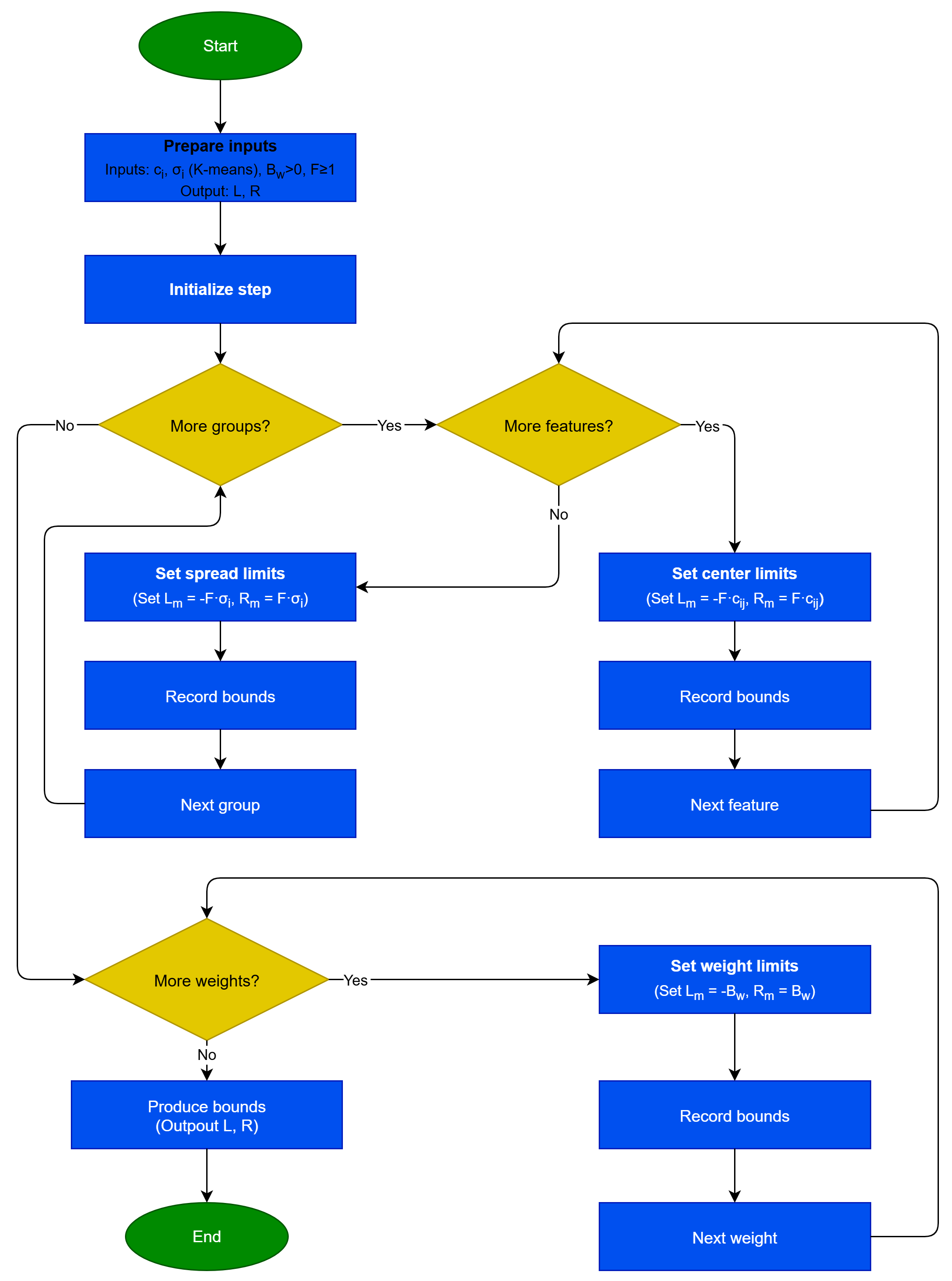
The algorithm depicted graphically in Figure 3 describes a procedure for computing safe parameter bounds informed by K-means. The process begins by preparing the inputs, the cluster centroids and spreads, a positive initial bound for the weights, and a scaling factor $F\ge 1$, aiming to produce the lower and upper bound vectors L and R. For each group and for each of its features, symmetric bounds around zero are computed as F times the corresponding centroid coordinate (i.e., $L_m=-F\times c_{ij},R_m=F\times c_{ij}$). After completing a group’s features, a complementary step computes bounds based on that group’s spread, using $F\times {\sigma }_i$ (i.e., $L_m=-F\times {\sigma }_i,R_m=F\times {\sigma }_i$). In this way, every group receives a complete, consistent specification through two contributions: one driven by feature centroids and one capturing group extent. Once all groups have been processed, initial bounds for the combining weights are assigned using a fixed symmetric limit $B_w$ (i.e., $L_m=-B_w,R_m=B_w$). Finally, all computed limits are assembled into L and R, ready for training, estimation, or validity checks. The overall logic is hierarchical and layered: leveraging centroid information, incorporating spread, and bounding the weights, with clear and reproducible steps throughout the flow.

3.2. The Description for the Second Phase

During the second phase, an optimization procedure is utilized to minimize Equation (3) considering the bound vectors $\overrightarrow{L},\overrightarrow{R}$ of the previous phase. In the proposed implementation, the genetic algorithm was incorporated during the second phase. Genetic algorithms are evolutionary methods that are based on randomly produced solutions of the objective problem. The candidate solutions in a genetic algorithm are typically referred to as chromosomes, and they evolve through operations inspired by natural processes, such as selection, crossover, and mutation. They have been incorporated into a wide series of problems, such as energy problems [46], water distribution [47], problems appearing in banking transactions [48], optimization of neural networks [49], etc. Also, another advantage of genetic algorithms is that they can easily adopt parallel programming techniques in order to speed up the evolutionary process [50,51]. Figure 4 illustrates the structure of the chromosomes involved in the genetic algorithm in this phase. In this figure the following assumptions hold:

• The value $c_{i,j}$ denotes the j element of the i center of the RBF network, with $i\in [1,k]$ and $j\in [1,d].$
• The value ${\sigma }_i$ represents the $\sigma$ parameter for the corresponding radial function.
• The value $w_i,i\in [1,k]$ represents the weight for the corresponding radial function.

The following steps outline the proposed genetic algorithm:

• Initialization step.

  (a)

  The following set of parameters is initialized: $N_c$ for the number of chromosomes; $N_g$, used to express the maximum number of allowed generations; $p_s$, which defines the selection rate; and finally $p_m$, which is used to represent the mutation rate.

  (b)

  The chromosomes in the proposed genetic algorithm are initialized as random decimal numbers that follow the configuration of Figure 4, and the initialization is performed within the value range of the first phase, which is defined by the vectors $\overrightarrow{L},\overrightarrow{R}$.

  (c)

  Set $k=0$. This variable denotes the number of generations.

• Fitness calculation step.

  (a)

  For $i=1,\dots ,N_c$ perform the following:

  • Produce an RBF network $R_i=R\left(\overrightarrow{x},\overrightarrow{g_i}\right).$ The parameters of this network are stored in the chromosome $\overrightarrow{g_i}.$
  • Estimate the related fitness $f_i$ as

    $$f_i=\sum _{j=1}^M{\left(R\left({\overrightarrow{x}}_j,\overrightarrow{g_i}\right)-y_j\right)}^2$$

    (5)

  (b)

  End For.

• Genetic operation step.

  (a)

  Selection procedure: Initially, all chromosomes are sorted based on their fitness values. The top $p_s\times N_c$ chromosomes are directly carried over to the next generation without any modification. The remaining individuals are replaced by offspring generated through crossover and mutation operations.

  (b)

  Crossover procedure: During this procedure $\left(1-p_s\right)\times N_c$ new chromosomes are constructed. For each pair $\left(\tilde{z},\tilde{w}\right)$ of new chromosomes, two chromosomes $(z,w)$ are chosen using tournament selection. The new offsprings are produced following the scheme

  $$\begin{array}{ccc}\hfill \widetilde{z_i}& =& a_i{z}_i+\left(1-a_i\right)w_i\hfill \\ \hfill \widetilde{w_i}& =& a_i{w}_i+\left(1-a_i\right)z_i\hfill \end{array}$$

  (6)

  The numbers $a_i$ are considered random numbers in the range $[-0.5,1.5]$ [52].

  (c)

  Mutation procedure: A random number $r\in [0,1]$ is picked for each element $t_j,j=1,\dots ,n$ and for every chromosome $g_i$. If $r\le p_m$, then this element is altered according to the following equation:

  $$t_j^{\prime }=\left\{\begin{array}{cc}{t}_j+\Delta \left(k,R_j-t_j\right),\hfill & t=0\hfill \\ t_j-\Delta \left(k,t_j-L_j\right),\hfill & t=1\hfill \end{array}\right.$$

  (7)

  The value t is a random number that can be either 0 or 1. The function $\Delta (k,y)$ is provided by the following equation:

  $$\Delta (k,y)=y\left(1-r^{\left(1-{\displaystyle \frac{k}{N_g}}\right)}\right)$$

  (8)

• Termination check step.

  (a)

  Set $k=k+1$.

  (b)

  If $k<N_g$ then the procedure returns to the fitness calculation step.

  (c)

  Otherwise, the best chromosome $g^{*}$ is returned as the result of the algorithm.

3.3. The Steps of the Third Phase

In the third phase of the present work, a local optimization procedure is applied to the results of the previous phase to identify an actual minimum of the RBF network’s training error. In this work, Powell’s [53] BFGS variant was utilized as the local optimization method. This variant can preserve the bounds located previously in an efficient way. During the past years a series of modifications to the BFGS method have been introduced, such as the limited memory variant L-BFGS ideal for large-scale problems [54] or the Regularized Stochastic BFGS Algorithm [55]. Also, Dai published an article on the convergence properties of the BFGS method [56]. The main steps of the final phase of the algorithm are as follows:

• Obtain the best chromosome $\overrightarrow{g^{*}}$ of the previous phase.
• Produce the RBF network that corresponds to this chromosome, denoted as $R^{*}=R\left(\overrightarrow{x},\overrightarrow{g^{*}}\right)$.
• Minimize the training error of the network $R^{*}$ using the local search procedure of this phase.
• The network $R^{*}$ is applied to the test set and the corresponding classification or regression error is calculated and reported.

A summary flow chart showing the sequence of the various phases of the proposed work is presented in Figure 5.

3.4. The Experimental Datasets

The proposed method was evaluated on a broad set of classification and regression problems, available from the UCI database [57], the KEEL database [58], and the STATLIB database [59]. The classification datasets used in the experiments, along with their details (number of patterns and classes), are summarized in

Table 1. The column ‘DATASET’ indicates the name of each dataset. The ‘Reference Paper’ column refers to the publication in which the dataset was mentioned. The ‘Patterns’ column shows the number of patterns in the dataset, while the ‘Number of Classes’ column represents the number of distinct classes contained in the dataset.

DATASET	Reference Paper	Patterns	Number of Classes
APPENDICITIS	[60]	106	2
ALCOHOL	[61]	476	4
AUSTRALIAN	[62]	690	2
BALANCE	[63]	625	3
CLEVELAND	[64,65]	297	5
CIRCULAR	[66]	500	2
DERMATOLOGY	[67]	368	6
ECOLI	[68]	336	8
HAYES ROTH	[69]	132	3
HEART	[70]	270	2
HEARTATTACK	[71]	303	2
HOUSEVOTES	[72]	232	2
IONOSPHERE	[73,74]	351	2
LIVERDISORDER	[75,76]	345	2
LYMOGRAPHY	[77]	148	4
MAMMOGRAPHIC	[78]	830	2
PARKINSONS	[79]	195	2
PIMA	[80]	768	2
POPFAILURES	[81]	540	2
REGIONS2	[82]	622	5
SAHEART	[83]	462	2
SEGMENT	[84]	2300	7
SPIRAL	[66]	2000	2
STATHEART	[85]	270	2
STUDENT	[86]	403	2
TRANSFUSION	[87]	748	2
WDBC	[88,89]	569	2
WINE	[90,91]	179	3
Z_F_S	[92,93]	300	3
Z_O_N_F_S	[92,93]	500	5
ZO_NF_S	[92,93]	500	3
ZONF_S	[92,93]	500	2
ZOO	[94]	101	7

.

Also,

Table 2. The list of regression datasets.

DATASET	Reference Paper	Patterns
ABALONE	[95]	4177
AIRFOIL	[96]	1483
AUTO	[97]	392
BK	[66]	96
BL	[66]	43
BASEBALL	[58]	337
CONCRETE	[98]	1030
DEE	[58]	365
FA	[59]	252
FRIEDMAN	[99]	1200
FY	[59]	125
HO	[59]	506
HOUSING	[100]	506
LASER	[57]	993
LW	[59]	189
MORTGAGE	[58]	1049
PL	[59]	1650
PLASTIC	[57]	1670
QUAKE	[57]	2178
SN	[59]	576
STOCK	[58]	950
TREASURY	[58]	1049

presents the used regression datasets.

4. Results

4.1. Experimental Results

The experiments were conducted on a Debian Linux system with 128 GB of RAM, and all the necessary code was implemented in the C++ programming language. Also, the OPTIMUS computing environment [101], available from https://github.com/itsoulos/GlobalOptimus.git (accessed on 9 October 2025), was used for the optimization methods. Ten-fold cross-validation was employed to validate the experimental results. The average classification error is calculated as follows:

$$E_C\left(N\left(\overrightarrow{x},\overrightarrow{w}\right)\right)=100\times {\displaystyle \frac{{\sum }_{i=1}^N\left(\mathrm{class}\left(N\left(\overrightarrow{x_i},\overrightarrow{w}\right)\right)-y_i\right)}{N}}$$

(9)

The set T denotes the associated test set, where $T=\left(x_i,y_i\right),i=1,\dots ,N$. Similarly, the average regression error has the following definition:

$$E_R\left(N\left(\overrightarrow{x},\overrightarrow{w}\right)\right)={\displaystyle \frac{{\sum }_{i=1}^N{\left(N\left(\overrightarrow{x_i},\overrightarrow{w}\right)-y_i\right)}^2}{N}}$$

(10)

Table 3. The values for each parameter of the proposed method.

NAME	MEANING	VALUE
k	Number of radial functions	10
F	Scaling factor	$2.0$
$B_w$	Bound value for the weights	$10.0$
$N_c$	Chromosomes	500
$N_g$	Allowed number of generations	200
$p_s$	Selection rate	$0.1$
$p_m$	Mutation rate	$0.05$

contains the values for each parameter of this method.

In the results tables that follow, the columns and rows have the following meanings:

• The column DATASET is used to represent the name of the used dataset.
• The results from the incorporation of the BFGS procedure [102] to train an artificial neural network [103,104] with 10 weights are presented in the column under the title BFGS.
• The ADAM column presents the results obtained by training a 10-weight neural network using the ADAM local optimization technique [105,106].
• The column RBF-KMEANS is used here to denote the usage of the initial training method of RBF networks to train an RBF network with 10 nodes.
• The column NEAT (NeuroEvolution of Augmenting Topologies) [107] stands for the method NEAT incorporated in the training of neural networks.
• The column DNN stands for the incorporation of a deep neural network, as implemented in the Tiny Dnn library, which can be downloaded freely from https://github.com/tiny-dnn/tiny-dnn (accessed on 9 October 2025). The optimization method AdaGrad [108] was incorporated for the training of the neural network.
• The BAYES column presents results obtained using the Bayesian optimizer from the open-source BayesOpt library [109], applied to train a neural network with 10 processing nodes.
• The column GENRBF stands for the method introduced in [110] for RBF training.
• The column PROPOSED is used to represent the results obtained by the current work.
• The row denoted as AVERAGE summarizes the mean regression or classification error calculated over all datasets.
• In the experimental results, boldface highlighting was used to make it clear which of the machine learning techniques has the lowest error on each dataset.

Table 4. The experimental outcomes on the classification datasets achieved with the machine learning techniques presented in this section.

DATASET	BFGS	ADAM	NEAT	DNN	BAYES	RBF-KMEANS	GENRBF	PROPOSED
Alcohol	41.50%	57.78%	66.80%	39.04%	30.85%	49.38%	52.45%	28.57%
Appendicitis	18.00%	16.50%	17.20%	17.30%	15.00%	12.23%	16.83%	15.00%
Australian	38.13%	35.65%	31.98%	35.03%	34.83%	34.89%	41.79%	22.67%
Balance	8.64%	7.87%	23.14%	24.56%	8.13%	33.42%	38.02%	13.11%
Cleveland	77.55%	67.55%	53.44%	63.28%	64.79%	67.10%	67.47%	50.86%
Circular	6.08%	19.95%	35.18%	21.87%	21.06%	5.98%	21.43%	5.13%
Dermatology	52.92%	26.14%	32.43%	24.26%	49.80%	62.34%	61.46%	36.00%
Hayes Roth	37.33%	59.70%	50.15%	44.65%	59.39%	64.36%	63.46%	38.31%
Heart	39.44%	38.53%	39.27%	30.67%	30.85%	31.20%	28.44%	16.07%
HeartAttack	46.67%	45.55%	32.34%	32.97%	33.93%	29.00%	40.48%	19.20%
HouseVotes	7.13%	7.48%	10.89%	3.13%	8.39%	6.13%	11.99%	3.65%
Ionosphere	15.29%	16.64%	19.67%	12.57%	15.03%	16.22%	19.83%	12.17%
Liverdisorder	42.59%	41.53%	30.67%	32.21%	34.21%	30.84%	36.97%	29.29%
Lymography	35.43%	29.26%	33.70%	24.07%	25.50%	25.50%	29.33%	24.36%
Mammographic	17.24%	46.25%	22.85%	19.83%	21.15%	21.38%	30.41%	17.79%
Parkinsons	27.58%	24.06%	18.56%	21.32%	19.32%	17.41%	33.81%	17.53%
Pima	35.59%	34.85%	34.51%	32.63%	35.52%	25.78%	27.83%	24.02%
Popfailures	5.24%	5.18%	7.05%	6.83%	7.63%	7.04%	7.08%	6.33%
Regions2	36.28%	29.85%	33.23%	33.42%	30.16%	38.29%	39.98%	26.29%
Saheart	37.48%	34.04%	34.51%	35.11%	34.87%	32.19%	33.90%	28.50%
Segment	68.97%	49.75%	66.72%	32.04%	51.70%	59.68%	54.25%	45.00%
Sonar	25.85%	30.33%	34.10%	20.50%	27.15%	27.90%	37.13%	22.00%
Spiral	47.99%	48.90%	50.22%	45.64%	50.57%	44.87%	50.02%	13.26%
Statheart	39.65%	44.04%	44.36%	30.22%	31.41%	31.36%	42.94%	19.67%
Student	7.14%	5.13%	10.20%	6.93%	5.83%	5.49%	33.26%	5.23%
Transfusion	25.84%	25.68%	24.87%	25.92%	25.41%	26.41%	25.67%	26.04%
Wdbc	29.91%	35.35%	12.88%	9.43%	9.52%	7.27%	8.82%	5.54%
Wine	59.71%	29.40%	25.43%	27.18%	21.77%	31.41%	31.47%	9.47%
Z_F_S	39.37%	47.81%	38.41%	9.27%	17.63%	13.16%	23.37%	3.73%
Z_O_N_F_S	65.67%	78.79%	77.08%	67.80%	54.08%	48.70%	68.40%	41.00%
ZO_NF_S	43.04%	47.43%	43.75%	8.50%	20.02%	9.02%	22.18%	4.24%
ZONF_S	15.62%	11.99%	5.44%	2.52%	3.10%	4.03%	17.41%	1.98%
ZOO	10.70%	14.13%	20.27%	16.20%	14.70%	21.93%	33.50%	9.80%
AVERAGE	33.50%	33.73%	32.77%	25.52%	27.21%	28.54%	34.89%	19.45%

compares the performance of eight methods on thirty-three classification datasets. The mean percentage error clearly shows that the proposed method is best overall at 19.45%, followed by DNN at 25.52% and then BAYES at 27.21%, RBF-KMEANS at 28.54%, NEAT at 32.77%, BFGS at 33.50%, ADAM at 33.73%, and GENRBF at 34.89%. Relative to the strongest competitor, DNN, the proposed method lowers the average error by 6.07 points, about 24%. The reduction versus the classical BFGS and ADAM is about 14 points, roughly 42%, and versus RBF-KMEANS about 9.1 points, roughly 32%.

At the level of individual datasets, the proposed method delivers strikingly low errors in several cases. On Spiral, it drops to 13.26% while others are around 45–50%; on Wine it reaches 9.47% versus 21–60%; and on Wdbc it achieves 5.54% versus 7–35%. On Z_F_S, ZO_NF_S, ZONF_S, and Cleveland it attains the best or tied-best results. On Heart, HeartAttack, Statheart, Regions2, Saheart, Pima, Australian, Alcohol, and HouseVotes, the results are also highly competitive, usually best or within the top two. There are, however, datasets where other methods prevail: DNN clearly leads on Segment and HouseVotes and is very strong on Dermatology; RBF-KMEANS is best on Appendicitis; and ADAM wins narrowly on Student and Balance. In cases like Balance, Popfailures, Dermatology, and Segment, the proposed method is not the top performer, though it remains competitive.

In summary, the proposed method not only attains the lowest average error but also consistently outperforms a broad range of classical and contemporary baseline methods. Despite local exceptions where DNN, ADAM, or RBF-KMEANS come out ahead, the approach appears more generalizable and stable, achieving systematically low errors and large improvements on challenging datasets, which supports its practical use as a default choice for classification.

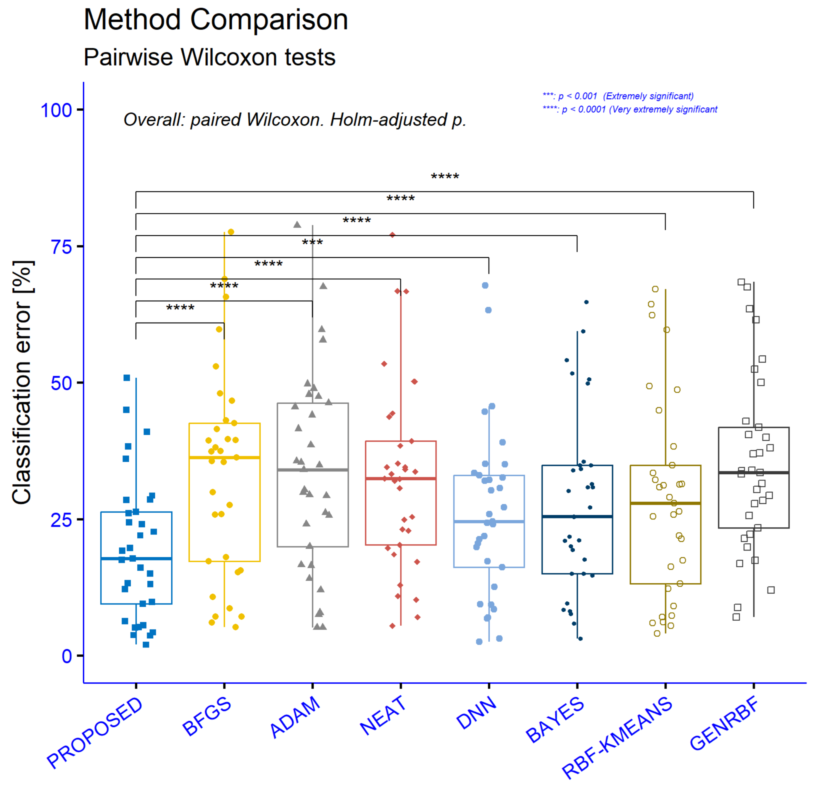
Figure 6 and

Table 5. Pairwise Wilcoxon results: proposed vs. baselines on classification datasets (95% CI and effect size).

Comparison	n	V	${\mathit{r}}_{\mathit{rank},\mathit{biserial}}$	${\mathit{conf}}_{\mathit{low}}$	${\mathit{conf}}_{\mathit{high}}$	p	${\mathit{p}}_{\mathit{adj}}$	${\mathit{p}}_{\mathit{signif}}$
PROPOSED vs. BFGS	33	26	−0.954	−18.51	−7.96	5.67 × 10−7	1.70 × 10−6	****
PROPOSED vs. ADAM	33	32	−0.943	−19.42	−8.03	9.37 × 10−7	1.87 × 10−6	****
PROPOSED vs. NEAT	33	11	−0.980	−18.40	−7.15	1.54 × 10−7	9.22 × 10−7	****
PROPOSED vs. DNN	33	66	−0.882	−8.93	−3.09	1.31 × 10−4	3.22 × 10−4	***
PROPOSED vs. BAYES	32	17	−0.968	−10.22	−4.90	4.04 × 10−7	1.62 × 10−6	****
PROPOSED vs. RBF-KMEANS	33	13	−0.977	−12.11	−4.90	1.84 × 10−7	9.22 × 10−7	****
PROPOSED vs. GENRBF	33	1	−0.998	−19.12	−12.01	6.19 × 10−8	4.33 × 10−8	****

***: $p<0.001$ (extremely significant), ****: $p<0.0001$ (very extremely significant).

summarize paired Wilcoxon signed-rank tests comparing the PROPOSED method against each competitor on the same 33 classification datasets. In all statistical figures The asterisks correspond to p-value thresholds as follows:

• ns: p > 0.05 (not statistically significant)
• *: $p<0.05$ (significant)
• **: $p<0.01$ (highly significant)
• ***: $p<0.001$ (extremely significant)
• ****: $p<0.0001$ (very extremely significant)

The column n is the number of paired datasets, V is the Wilcoxon signed-rank statistic, $r_{rank,biserial}$ is the rank-biserial effect size (range −1 to 1, with more a negative value meaning PROPOSED has a lower error), $con{f}_{low}$ and $con{f}_{high}$ give the 95% Hodges–Lehmann confidence interval for the median paired difference (PROPOSED–competitor) in percentage point error, p is the raw p-value, $p_{adj}$ is the Holm-adjusted p-value, and $p_{signif}$ is the significance code. Because all confidence intervals are entirely negative, the PROPOSED method consistently shows a lower error than each baseline, not just statistical significance but a stable direction of effect across datasets. Adjusted p-values remain very small in every comparison, from $4.33\times {10}^{-6}$ (vs. GENRBF) up to $1.31\times {10}^{-4}$ (vs. DNN), yielding **** everywhere except the DNN comparison, which is ***. Effect sizes are uniformly large in magnitude. The strongest difference is against GENRBF, with r ≈ −0.998 and a 95% CI for the median error reduction of roughly −19.12 to −12.01 percentage points. Very large effects also appear versus NEAT (r ≈ −0.980, CI ≈ [−18.40, −7.15]) and RBF-KMEANS (r ≈ —0.977, CI ≈ [−12.11, −4.90]). Comparisons with BFGS (r ≈ −0.954, CI ≈ [−18.51, −7.96]) and ADAM (r ≈ −0.943, CI ≈ [−19.42, −8.03]) remain strongly favorable. The smallest, yet still large, effect is against DNN (r ≈ −0.882), with a clearly negative CI ≈ [−8.93, −3.09]. Taken together, the results show consistent, substantial reductions in classification error for the PROPOSED method across all baselines, with very large effect sizes, tight negative confidence intervals, and significance that survives multiple-comparison correction.

Table 6. Comparison of precision and recall between the conventional RBF training approach and the proposed technique.

	RBF-KMEANS		PROPOSED
DATASET	PRECISION	RECALL	PRECISION	RECALL
Alcohol	0.507	0.639	0.723	0.711
Appendicitis	0.762	0.875	0.804	0.722
Australian	0.604	0.669	0.779	0.756
Balance	0.753	0.741	0.794	0.86
Cleveland	0.268	0.385	0.39	0.392
Circular	0.941	0.948	0.963	0.962
Dermatology	0.305	0.357	0.642	0.589
Hayes Roth	0.34	0.378	0.68	0.632
Heart	0.69	0.688	0.839	0.831
HeartAttack	0.668	0.674	0.779	0.774
HouseVotes	0.938	0.94	0.962	0.966
Ionosphere	0.806	0.847	0.889	0.868
Liverdisorder	0.665	0.673	0.689	0.684
Lymography	0.688	0.742	0.783	0.774
Mammographic	0.793	0.793	0.826	0.826
Parkinsons	0.685	0.8	0.758	0.747
Pima	0.679	0.732	0.744	0.705
Popfailures	0.501	0.93	0.792	0.735
Regions2	0.331	0.502	0.645	0.506
Saheart	0.607	0.641	0.669	0.645
Segment	0.4	0.433	0.603	0.579
Sonar	0.716	0.722	0.805	0.792
Spiral	0.553	0.555	0.868	0.869
Statheart	0.689	0.695	0.797	0.793
Student	0.944	0.955	0.949	0.95
Transfusion	0.533	0.641	0.618	0.534
Wdbc	0.912	0.929	0.952	0.943
Wine	0.676	0.763	0.919	0.907
Z_F_S	0.865	0.871	0.954	0.96
Z_O_N_F_S	0.534	0.52	0.621	0.61
ZO_NF_S	0.9	0.9	0.956	0.6
ZONF_S	0.926	0.947	0.966	0.976
ZOO	0.804	0.809	0.875	0.878
AVERAGE	0.667	0.718	0.789	0.76

further illustrates the comparison of precision and recall on the classification datasets between the conventional RBF training method and the proposed technique.

Table 7. Results from the regression datasets, generated using the machine learning methods described in this work.

DATASET	BFGS	ADAM	NEAT	DNN	BAYES	RBF-KMEANS	GENRBF	PROPOSED
Abalone	5.69	4.30	9.88	6.91	4.81	7.37	9.98	6.12
Airfoil	0.003	0.005	0.067	0.004	0.004	0.27	0.121	0.004
Auto	60.97	70.84	56.06	13.26	27.03	17.87	16.78	8.81
Baseball	119.63	77.90	100.39	110.22	88.76	93.02	98.91	88.05
BK	0.28	0.03	0.15	0.02	0.023	0.02	0.023	0.022
BL	2.55	0.28	0.05	0.006	0.46	0.013	0.005	0.0004
Concrete	0.066	0.078	0.081	0.021	0.013	0.011	0.015	0.005
Dee	2.36	0.630	1.512	0.31	0.28	0.17	0.25	0.15
Housing	97.38	80.20	56.49	65.18	57.39	57.68	95.69	15.36
Friedman	1.26	22.90	19.35	2.75	3.79	7.23	16.24	5.99
FA	0.426	0.11	0.19	0.02	0.051	0.015	0.15	0.013
FY	0.22	0.038	0.08	0.039	0.21	0.041	0.041	0.054
HO	0.62	0.035	0.169	0.026	0.034	0.03	0.076	0.009
Laser	0.015	0.03	0.084	0.045	0.026	0.03	0.075	0.016
Mortgage	8.23	9.24	14.11	9.74	3.01	1.45	1.92	0.23
PL	0.29	0.117	0.098	0.056	0.056	2.12	0.155	0.023
Plastic	20.32	11.71	20.77	3.82	3.66	8.62	25.91	2.28
PY	0.578	0.09	0.075	0.028	0.401	0.012	0.029	0.021
Quake	0.42	0.06	0.298	0.04	0.093	0.07	0.79	0.036
SN	0.40	0.026	0.174	0.032	0.055	0.027	0.027	0.026
Stock	302.43	180.89	12.23	39.08	14.43	12.23	25.18	1.44
Treasury	9.91	11.16	15.52	13.76	3.74	2.02	1.89	0.47
AVERAGE	28.82	21.39	13.99	11.82	9.18	9.56	13.38	5.87

evaluates the performance of eight regression methods on twenty-one datasets using absolute errors. The average error shows a clear overall advantage for the proposed method at 5.87, followed by BAYES at 9.18, RBF-KMEANS at 9.56, DNN at 11.82, NEAT at 13.99, GENRBF at 13.38, ADAM at 21.39, and BFGS at 28.82. Relative to the best-competing average, BAYES, the proposed method reduces the error by about 3.31 points (≈36%). The reduction versus RBF-KMEANS is about 3.69 points (≈39%), versus DNN about 5.95 points (≈50%), and relative to NEAT and GENRBF the drops are roughly 58% and 56%, respectively. The advantage is even larger against ADAM and BFGS, where the mean error is nearly halved or more.

Across individual datasets, the proposed method attains the best value in roughly two thirds of the cases. It is clearly first on Auto, BL, Concrete, Dee, Housing, FA, HO, Mortgage, PL, Plastic, Quake, Stock, and Treasury, with particularly large margins on Housing and Stock where errors fall to 15.36 and 1.44 while other methods range from tens to hundreds. On Airfoil it is essentially tied with the best at 0.004, while BFGS is slightly lower at 0.003. There are datasets where other methods lead, such as Abalone where ADAM and BAYES are ahead; Friedman and Laser where BFGS gives the best value; BK where DNN and RBF-KMEANS lead; and PY where RBF-KMEANS is lower. Despite these isolated exceptions, the proposed method remains consistently among the top performers and most often the best.

Overall, the proposed approach combines a very low average error with broad superiority across diverse problem types and error scales, from thousandths to very large magnitudes. The consistency of the gains and the size of the margins over all baselines indicate that it is the most efficient and generalizable choice among the regression methods considered.

Figure 7 and

Table 8. Pairwise Wilcoxon results: proposed vs. baselines on regression datasets (95% CI and effect size).

Comparison	n	V	${\mathit{r}}_{\mathit{rank},\mathit{biserial}}$	${\mathit{conf}}_{\mathit{low}}$	${\mathit{conf}}_{\mathit{high}}$	p	${\mathit{p}}_{\mathit{adj}}$	${\mathit{p}}_{\mathit{signif}}$
PROPOSED vs. BFGS	22.00	28.00	−0.889	−20.51	−0.316	1.46 × 10−3	5.54 × 10−3	**
PROPOSED vs. ADAM	21.00	33.00	−0.857	−27.34	−0.416	4.37 × 10−3	6.27 × 10−3	**
PROPOSED vs. NEAT	22.00	0.00	−1.000	−9.93	−0.160	4.30 × 10−4	3.01 × 10−3	***
PROPOSED vs. DNN	21.00	23.00	−0.900	−11.09	−0.012	1.39 × 10−3	5.54 × 10−3	**
PROPOSED vs. BAYES	21.00	30.00	−0.870	−5.84	−0.335	3.13 × 10−3	6.27 × 10−3	**
PROPOSED vs. RBF-KMEANS	22.00	14.00	−0.945	−4.52	−0.034	2.77 × 10−4	1.38 × 10−3	***
PROPOSED vs. GENRBF	22.00	6.00	−0.976	−10.25	−0.098	9.77 × 10−4	5.86 × 10−4	***

**: $p<0.01$ (highly significant), ***: $p<0.001$ (extremely significant).

summarize paired Wilcoxon signed-rank tests between PROPOSED and each method on the same regression datasets. In every comparison the 95% confidence interval is entirely negative, so PROPOSED consistently attains a lower error than each baseline. Holm-adjusted p-values range from about $5.86\times {10}^{-4}$ to 0.0063, yielding ** or *** across all pairings, indicating strong though not extreme significance. Effect sizes are very large in absolute value, implying a consistent sign of the differences across datasets. The strongest dominance is against NEAT with r ≈ −1 and V = 0, meaning that in every non-tied pair PROPOSED was better, with a confidence interval of roughly [−9.93, −0.16]. Similarly large effects appear against GENRBF (r ≈ −0.976, CI [−10.25, −0.098]) and RBF-KMEANS (r ≈ −0.945, CI [−4.52, −0.034]); the upper bound near zero indicates that the typical improvement can range from very small to several points depending on the dataset. Against BFGS and ADAM the effects remain very large (r ≈ −0.889 and r ≈ −0.857, respectively) with wider intervals [−20.51, −0.316] and [−27.34, −0.0416], showing substantial heterogeneity in the magnitude of error reduction while the direction remains in favor of PROPOSED. The most challenging comparison is with DNN: although |r| is still very large (≈0.900), the CI is narrow and close to zero [−11.09, −0.012], implying that while superiority is consistent, the typical error reduction may be small in many cases.

Overall, the results demonstrate that PROPOSED systematically outperforms all alternatives on regression, with very large rank-based effect sizes, negative and robust confidence intervals, and significance that survives multiple-comparison correction. The strength of the improvement varies by problem and is more modest against DNN, but the direction of the effect is consistently in favor of PROPOSED across all comparisons.

4.2. Experiments with Different Values of Scale Factor F

In order to evaluate the stability and reliability of the current work when its critical parameters are altered, a series of additional experiments were executed. In one of them, the stability of the technique was studied with the change in the scale factor F. This factor regulates the range of network parameter values and is scaled as a multiple of the initial estimates obtained from the first-phase K-means method. In this series of experiments, the value of F was altered in the range $[1,8]$.

The effect of the scale factor F on the performance of the proposed machine learning model is presented in

Table 9. Results of applying the proposed method to the classification datasets, with the critical parameter F ranging between 1 and 8.

DATASET	$\mathit{F}=1$	$\mathit{F}=2$	$\mathit{F}=4$	$\mathit{F}=8$
Alcohol	28.83%	28.57%	28.83%	30.09%
Appendicitis	14.60%	15.00%	14.40%	15.50%
Australian	24.04%	22.67%	21.52%	20.59%
Balance	21.03%	13.11%	11.87%	11.44%
Cleveland	50.45%	50.86%	51.59%	50.90%
Circular	4.13%	5.13%	3.67%	3.49%
Dermatology	38.34%	36.00%	35.83%	34.97%
Hayes Roth	51.85%	38.31%	32.62%	33.92%
Heart	17.26%	16.07%	15.63%	15.30%
HeartAttack	22.07%	19.20%	19.30%	19.07%
HouseVotes	4.13%	3.65%	3.39%	4.81%
Ionosphere	14.69%	12.17%	8.83%	7.51%
Liverdisorder	29.35%	29.29%	28.53%	29.23%
Lymography	26.86%	24.36%	18.07%	19.86%
Mammographic	18.21%	17.79%	16.75%	17.05%
Parkinsons	18.32%	17.53%	15.68%	14.05%
Pima	23.53%	24.02%	23.72%	23.26%
Popfailures	7.83%	6.33%	5.15%	4.69%
Regions2	26.27%	26.29%	26.15%	25.73%
Saheart	29.24%	28.50%	28.74%	29.41%
Segment	45.08%	45.00%	42.14%	42.10%
Sonar	32.90%	22.00%	18.75%	18.05%
Spiral	12.03%	13.26%	16.66%	23.56%
Statheart	19.30%	19.67%	20.00%	19.44%
Student	6.33%	5.23%	5.10%	5.55%
Transfusion	25.54%	26.04%	25.66%	24.42%
Wdbc	4.86%	5.54%	5.75%	5.29%
Wine	12.18%	9.47%	8.59%	7.65%
Z_F_S	4.37%	3.73%	3.73%	3.37%
Z_O_N_F_S	39.80%	41.00%	40.04%	40.80%
ZO_NF_S	4.26%	4.24%	4.58%	3.78%
ZONF_S	2.52%	1.98%	2.58%	1.96%
ZOO	12.40%	9.80%	7.60%	6.90%
AVERAGE	20.99%	19.45%	18.53%	18.60%

. The parameter F takes four different values, 1, 2, 4, and 8, and for each dataset the classification error rate is reported. Analyzing the mean values, it is observed that $F=2$ and $F=4$ achieve the best overall performance, with average errors of 19.45% and 18.53%, respectively, compared to 20.99% for $F=1$ and 18.60% for $F=8$. This indicates that selecting an intermediate value of the initialization factor improves performance, reducing the error by about two percentage points relative to the baseline case of $F=1$. At the individual dataset level, interesting patterns emerge. For example, on Sonar the error drops significantly from 32.90% at $F=1$ to 18.75% at $F=4$, suggesting that the parameter F strongly influences performance in certain problems. In contrast, on Spiral increasing F worsens the results, as the error rises from 12.03% at $F=1$ to 23.56% at $F=8$. Similarly, on the Australian dataset a gradual increase in F from 1 to 8 systematically improves performance, reducing the error from 24.04% to 20.59%. Overall, the data show that the effect of the scale factor is not uniform across all problems, but the general trend indicates improvement when F increases from 1 to 2 or 4. Choosing $F=4$ appears to yield the best mean result, although the difference compared with $F=8$ is very small. Therefore, it can be concluded that tuning this parameter plays an important role in the stability and accuracy of the model and that intermediate values such as 4 constitute a good general choice.

Table 10. Results of applying the proposed method to the regression datasets, with the critical parameter F ranging between 1 and 8.

DATASET	$\mathit{F}=1$	$\mathit{F}=2$	$\mathit{F}=4$	$\mathit{F}=8$
Abalone	6.70	6.12	5.70	5.56
Airfoil	0.004	0.004	0.004	0.004
Auto	10.04	8.81	9.82	10.92
Baseball	87.01	88.05	85.87	86.76
BK	0.023	0.022	0.024	0.02
BL	0.01	0.0004	0.0002	0.00007
Concrete	0.008	0.005	0.005	0.006
Dee	0.15	0.15	0.16	0.16
Housing	14.64	15.36	17.34	18.48
Friedman	6.74	5.99	2.06	1.41
FA	0.012	0.013	0.012	0.013
FY	0.055	0.054	0.054	0.053
HO	0.009	0.009	0.01	0.009
Laser	0.027	0.016	0.005	0.0024
Mortgage	0.67	0.23	0.035	0.015
PL	0.023	0.023	0.023	0.022
Plastic	2.32	2.28	2.26	2.22
PY	0.019	0.021	0.013	0.011
Quake	0.036	0.036	0.036	0.036
SN	0.024	0.026	0.025	0.024
Stock	1.69	1.44	1.49	1.48
Treasury	0.57	0.47	0.035	0.031
AVERAGE	5.94	5.87	5.68	5.78

shows the effect of the scale factor F on the performance of the proposed regression model. Based on the mean errors, the best overall performance occurs at $F=4$ with an average error of 5.68, while the values for $F=1,F=2$ and $F=8$ are 5.94, 5.87, and 5.78, respectively. The differences across the four settings are not large, but they indicate that intermediate values and especially $F=4$ tend to offer the best accuracy–stability trade-off. At the level of individual datasets, substantial variations are observed. For Friedman the reduction is dramatic, with the error dropping from 6.74 at $F=1$ to 1.41 at $F=8$, highlighting that proper tuning of F can have a strong impact on performance. Laser shows a similarly large improvement, from 0.027 at $F=1$ to just 0.0024 at $F=8$. Mortgage also improves markedly, from $0.67$ at $F=1$ to 0.015 at $F=8$. By contrast, on some datasets the value of F has little practical effect, such as Quake and HO, where errors remain nearly constant regardless of F. There are also cases like Housing where increasing F degrades performance, with the error rising from 14.64 at $F=1$ to 18.48 at $F=8$. Overall, the results indicate that the scale factor F has a significant but nonuniform influence on model performance. On some datasets it sharply reduces error, while on others its impact is negligible or even negative. Nevertheless, the aggregate picture based on the mean errors suggests that $F=4$ and $F=8$ yield the most reliable results, with $F=4$ being the preferred choice for a general-purpose setting.

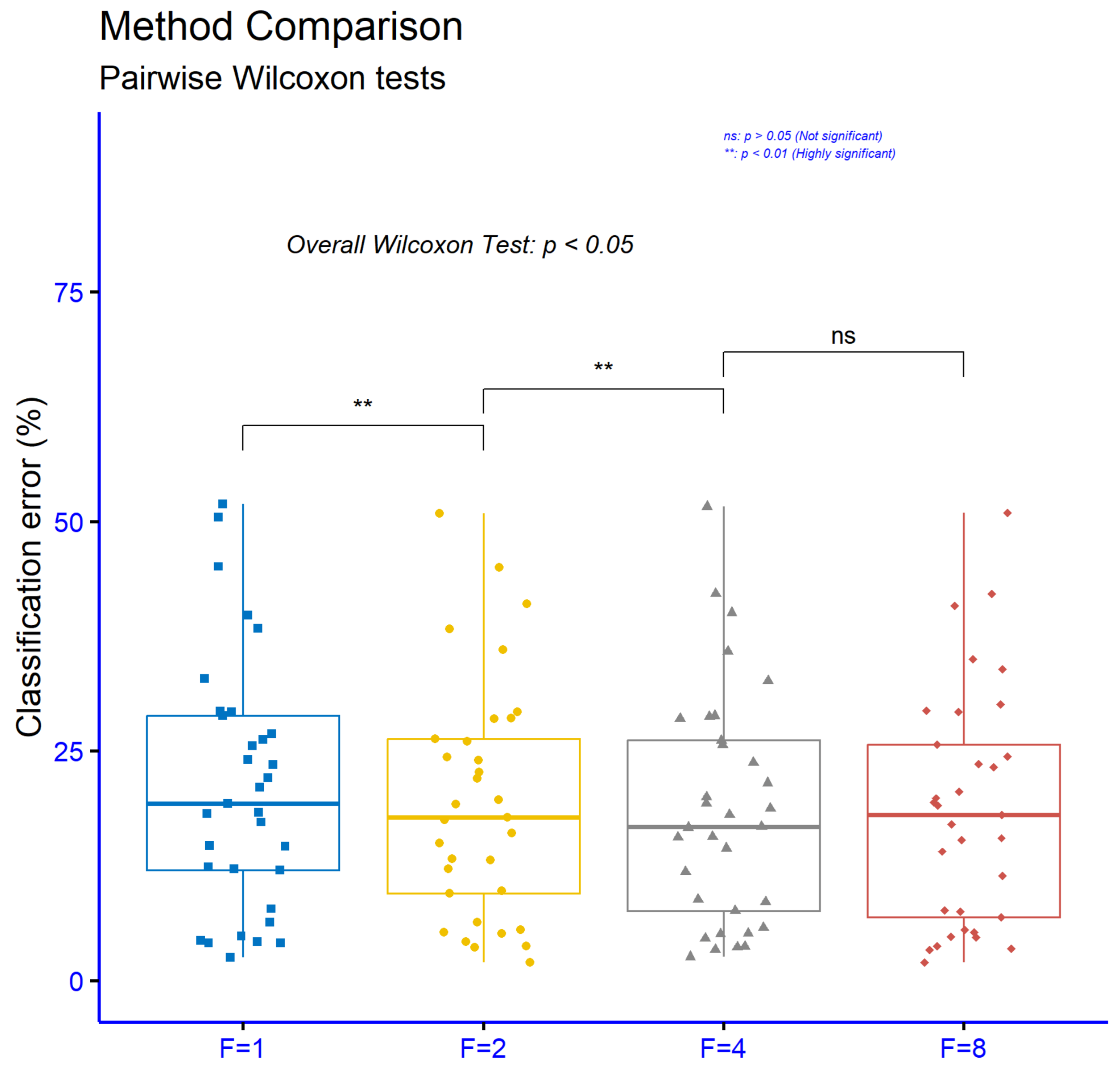
The significance levels for comparisons among different values of the parameter F in the proposed machine learning method, using the classification datasets, are shown in Figure 8. The analysis shows that the comparison between $F=1$ and $F=2$ results in high statistical significance with $p<0.01$, indicating that the transition from the initial value to $F=2$ has a substantial impact on performance. Similarly, the comparison between $F=2$ and $F=4$ also shows high statistical significance with $p<0.01$, suggesting that further increasing the parameter continues to positively affect the results. However, the comparison between $F=4$ and $F=8$ is characterized as not statistically significant, since $p>0.05$, which means that increasing the parameter beyond $F=4$ does not bring a meaningful difference in performance. Overall, the findings indicate that smaller values of F play a critical role in improving the model, while increases beyond 4 do not lead to further statistically significant improvements.

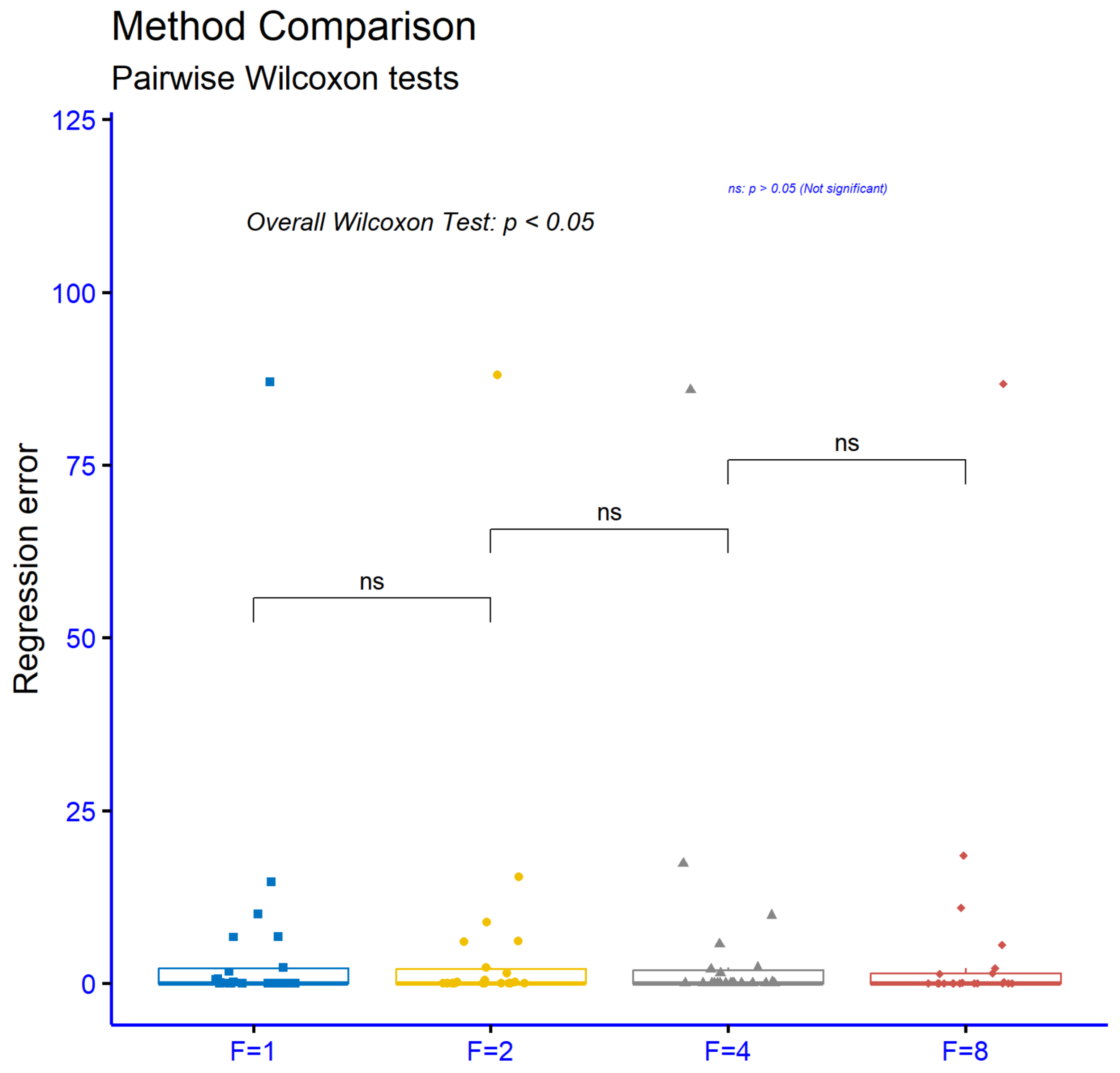
The significance levels for comparisons among different values of the parameter F in the proposed method, using the regression datasets, are presented in Figure 9. The results show that none of the comparisons $F=1$ vs. $F=2$, $F=2$ vs. $F=4$, and $F=4$ vs. $F=8$ exhibit statistically significant differences, since in all cases $p>0.05$. These results suggest that variations in the parameter F do not significantly influence the performance of the model on regression tasks. Therefore, it can be concluded that the choice of the F value is not of critical importance for these datasets and that the model remains stable regardless of the specific setting of this parameter.

4.3. Experiments with Differential Initialization Methods for Variances

The stability of the proposed method was also evaluated by employing a different procedure to determine the range of $\sigma$ parameters for the radial functions. Here, the $\sigma$ parameters were initially estimated using the variance calculated by the K-means algorithm. This calculation scheme is denoted as ${\sigma }_1$ in the following experimental tables. In this additional set of experiments, two more techniques were used, which will be denoted as ${\sigma }_{\mathrm{avg}}$ and ${\sigma }_{\max }$ in the following tables. In ${\sigma }_{\mathrm{avg}}$ the following calculation is performed:

$${\sigma }_{\mathrm{avg}}={\displaystyle \frac{1}{k}}\sum _{i=1}^k{\sigma }_i$$

(11)

Subsequently ${\sigma }_{\mathrm{avg}}$ is used to determine the range of values of the $\sigma$ parameters of the radial functions of the network. In ${\sigma }_{\mathrm{avg}}$ the following quantity is calculated:

$${\sigma }_{\max }=\max {\sigma }_i$$

(12)

This quantity is then employed to define the range of $\sigma$ parameter values for the radial functions.

Table 11. The proposed method was evaluated on the classification datasets using various approaches to compute the $\sigma$ parameters in the radial basis functions.

DATASET	${\mathsf{\sigma }}_1$	${\mathsf{\sigma }}_{\mathbf{avg}}$	${\mathsf{\sigma }}_{\mathbf{max}}$
Alcohol	28.57%	28.47%	26.17%
Appendicitis	15.00%	14.20%	15.70%
Australian	22.67%	25.14%	29.96%
Balance	13.11%	12.92%	12.23%
Cleveland	50.86%	51.76%	51.24%
Circular	5.13%	4.78%	4.45%
Dermatology	36.00%	37.54%	37.09%
Hayes Roth	38.31%	38.00%	35.69%
Heart	16.07%	16.52%	15.41%
HeartAttack	19.20%	19.70%	18.97%
HouseVotes	3.65%	3.31%	3.22%
Ionosphere	12.17%	13.00%	12.83%
Liverdisorder	29.29%	28.38%	27.77%
Lymography	24.36%	22.43%	23.50%
Mammographic	17.79%	17.28%	17.41%
Parkinsons	17.53%	14.74%	14.89%
Pima	24.02%	23.28%	23.91%
Popfailures	6.33%	6.37%	6.24%
Regions2	26.29%	25.47%	25.61%
Saheart	28.50%	28.89%	28.28%
Segment	45.00%	43.65%	46.36%
Sonar	22.00%	21.90%	21.30%
Spiral	13.26%	13.73%	13.37%
Statheart	19.67%	20.15%	19.00%
Student	5.23%	5.58%	5.23%
Transfusion	26.04%	22.78%	22.79%
Wdbc	5.54%	5.22%	5.21%
Wine	9.47%	7.93%	7.06%
Z_F_S	3.73%	3.70%	3.73%
Z_O_N_F_S	41.00%	40.20%	41.12%
ZO_NF_S	4.24%	4.42%	4.84%
ZONF_S	1.98%	1.92%	2.06%
ZOO	9.80%	12.50%	10.30%
AVERAGE	19.45%	19.27%	19.18%

presents the effect of three different calculation techniques for the $\sigma$ parameters used in the radial basis functions of the RBF model. The techniques are a fixed value ${\sigma }_1$, the mean distance-based initialization $\left({\sigma }_{\mathrm{avg}}\right)$, and the maximum distance-based initialization $\left({\sigma }_{\max }\right)$. Based on the mean errors, the maximum distance technique yields the lowest overall error at 19.18%. Very close is the mean distance technique at 19.27%, while the simple ${\sigma }_1$ initialization has a slightly higher error of 19.45%. Although the differences among the three approaches are small, the two adaptive methods $\left({\sigma }_{\mathrm{avg}}\mathrm{and}{\sigma }_{\max }\right)$ tend to produce marginally better overall performance. At the individual dataset level, behaviors vary. For example, on Wine the ${\sigma }_{\max }$ choice reduces error to 7.06%, far below the 9.47% obtained with ${\sigma }_1$. On Dermatology, ${\sigma }_1$ performs better than the other two, whereas on Segment the mean-based option is preferable. In some cases the differences are minor, e.g., Circular, Pima, and Popfailures, where all techniques are comparable; in others the choice of technique materially affects performance, as in Transfusion, where error drops from 26.04% with ${\sigma }_1$ to about 22.78% with the other two methods. Overall, the statistical picture indicates that no single technique dominates across all datasets. Nevertheless, methods that adapt $\sigma$ to the geometry of the data $\left({\sigma }_{\mathrm{avg}}\mathrm{and}{\sigma }_{\max }\right)$ tend to yield more reliable and stable results, while the fixed value lags slightly. The average differences are modest, but for certain problems the choice can significantly impact final performance.

Table 12. The proposed method was applied to the regression datasets, and results were analyzed using various approaches to compute the $\sigma$ parameters of the radial functions.

DATASET	${\mathsf{\sigma }}_1$	${\mathsf{\sigma }}_{\mathbf{avg}}$	${\mathsf{\sigma }}_{\mathbf{max}}$
Abalone	6.12	6.06	5.43
Airfoil	0.004	0.003	0.003
Auto	8.81	9.80	10.44
Baseball	88.05	86.13	85.89
BK	0.022	0.022	0.022
BL	0.0004	0.008	0.0004
Concrete	0.005	0.005	0.005
Dee	0.15	0.16	0.16
Housing	15.36	15.57	19.45
Friedman	5.99	6.21	6.02
FA	0.013	0.012	0.012
FY	0.054	0.055	0.055
HO	0.009	0.009	0.01
Laser	0.016	0.018	0.011
Mortgage	0.23	0.041	0.021
PL	0.023	0.022	0.022
Plastic	2.28	2.21	2.19
PY	0.021	0.02	0.022
Quake	0.036	0.036	0.036
SN	0.026	0.026	0.025
Stock	1.44	1.32	1.23
Treasury	0.47	0.15	0.08
AVERAGE	5.87	5.81	5.96

presents the effect of three different calculation techniques for the $\sigma$ parameters used in the radial basis functions of the RBF model. Based on the mean errors, the average distance method yields the lowest overall error at 5.81. Very close is the fixed value ${\sigma }_1$ with a mean error of 5.87, while the maximum distance method shows a slightly higher mean error of 5.96. The difference among the three methods is small, indicating that all can deliver comparable performance at a general level, with a slight advantage for the average distance approach. At the level of individual datasets, however, significant variations are observed. For example, on Mortgage the ${\sigma }_{\max }$ method reduces the error dramatically from 0.23 with ${\sigma }_1$ to 0.021, while ${\sigma }_{\mathrm{avg}}$ also provides a much better result with 0.041. On Treasury the improvement is again substantial, as the error decreases from 0.47 with ${\sigma }_1$ to just 0.08 using ${\sigma }_{\max }$. On Stock the reduction is clear, from 1.44 to 1.23, while on Plastic both ${\sigma }_{\mathrm{avg}}$ and ${\sigma }_{\max }$ yield lower errors than ${\sigma }_1$. On the other hand, on datasets such as Housing, the use of ${\sigma }_{\max }$ worsens performance, increasing the error from 15.36 with ${\sigma }_1$ to 19.45. Similarly, on Auto and Baseball the lowest errors are obtained with ${\sigma }_1$, whereas the alternative techniques result in slightly worse performance. Overall, the results show that the choice of calculation technique for $\sigma$ can significantly affect performance in certain problems, while in others the difference is negligible. Although no method consistently outperforms the others across all datasets, the average distance method appears slightly more reliable overall, while the maximum distance method can in some cases produce very large improvements but in others lead to a degradation in performance.

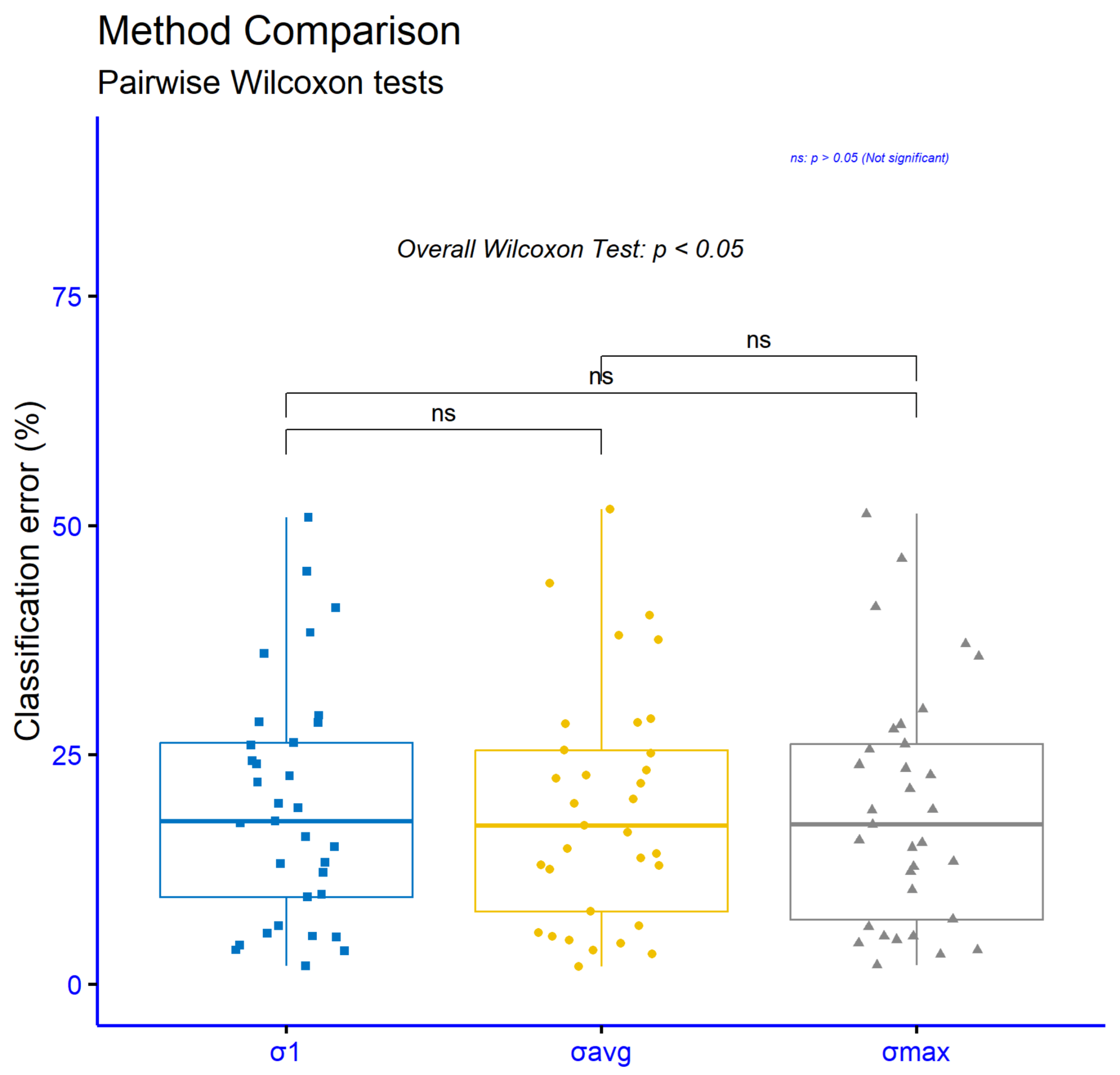
The significance levels for comparisons of various computation methods for the $\sigma$ parameters in the radial basis functions of the proposed model, using the classification datasets, are presented in Figure 10. The comparisons performed, ${\sigma }_1$ vs. ${\sigma }_{\mathrm{avg}}$, ${\sigma }_1$ vs. ${\sigma }_{\max }$, and ${\sigma }_{\mathrm{avg}}$ vs. ${\sigma }_{\max }$, did not show any statistically significant differences, since in all cases $p>0.05$. These results indicate that variations in the computation method for the $\sigma$ parameters do not significantly influence the performance of the model on classification tasks. Therefore, it can be concluded that the model maintains stable performance regardless of which of the three computation techniques is used.

The significance levels for comparisons of various methods for computing the $\sigma$ parameters in the radial basis functions of the proposed model, using the regression datasets, are presented in Figure 11. The comparisons examined, ${\sigma }_1$ vs. ${\sigma }_{\mathrm{avg}}$, ${\sigma }_1$ vs. ${\sigma }_{\max }$, and ${\sigma }_{\mathrm{avg}}$ vs. ${\sigma }_{\max }$, did not show any statistically significant differences, since in all cases $p>0.05$. This means that the choice of computation method for the $\sigma$ parameters does not have a substantial impact on the performance of the model in regression problems. Therefore, it can be concluded that the model demonstrates stable and consistent behavior regardless of which initialization technique is applied.

4.4. Experiments with the Number of Generations $N_g$

An additional experiment was executed, where the number of generations was altered from $N_g=50$ to $N_g=400$.

Table 13. The proposed method was applied to the classification datasets, and results were analyzed for varying numbers of generations $N_g$ ranging from 50 to 400.

DATASET	${\mathit{N}}_{\mathit{g}}=50$	${\mathit{N}}_{\mathit{g}}=100$	${\mathit{N}}_{\mathit{g}}=200$	${\mathit{N}}_{\mathit{g}}=400$
Alcohol	34.11%	31.32%	28.57%	27.02%
Appendicitis	14.90%	14.30%	15.00%	14.90%
Australian	25.23%	24.96%	22.67%	21.39%
Balance	14.98%	14.11%	13.11%	13.52%
Cleveland	52.00%	51.31%	50.86%	51.38%
Circular	3.75%	3.82%	5.13%	3.82%
Dermatology	47.86%	36.29%	36.00%	36.46%
Hayes Roth	40.54%	36.77%	38.31%	36.77%
Heart	16.19%	16.37%	16.07%	16.26%
HeartAttack	21.30%	21.63%	19.20%	20.07%
HouseVotes	4.09%	3.65%	3.65%	3.61%
Ionosphere	13.94%	12.57%	12.17%	11.17%
Liverdisorder	29.06%	29.23%	29.29%	29.06%
Lymography	22.14%	21.64%	24.36%	21.86%
Mammographic	17.19%	17.25%	17.79%	17.78%
Parkinsons	17.32%	17.11%	17.53%	17.63%
Pima	24.07%	24.38%	24.02%	24.28%
Popfailures	6.63%	5.92%	6.33%	6.15%
Regions2	26.02%	26.14%	26.29%	26.13%
Saheart	28.28%	28.63%	28.50%	29.61%
Segment	43.28%	42.70%	45.00%	41.35%
Sonar	22.65%	21.20%	22.00%	22.20%
Spiral	16.66%	14.47%	13.26%	12.45%
Statheart	20.22%	20.67%	19.67%	19.63%
Student	4.98%	4.85%	5.23%	5.45%
Transfusion	25.47%	25.32%	26.04%	25.84%
Wdbc	5.14%	4.84%	5.54%	5.39%
Wine	7.59%	8.53%	9.47%	10.24%
Z_F_S	4.13%	4.10%	3.73%	4.40%
Z_O_N_F_S	45.14%	43.04%	41.00%	38.26%
ZO_NF_S	4.14%	4.00%	4.24%	4.02%
ZONF_S	2.30%	2.36%	1.98%	2.02%
ZOO	17.10%	8.70%	9.80%	10.60%
AVERAGE	20.56%	19.46%	19.45%	19.11%

presents the effect of the number of generations $\left(N_g\right)$ on the performance of the proposed model. The overall trend is downward: the mean error decreases from 20.56% at 50 generations to 19.46% at 100, essentially stabilizes at 200 with 19.45%, and improves slightly further at 400 to 19.11%. Thus, the largest gain arrives early, from 50 to 100 generations (about 1.1 points), after which returns diminish, with small but tangible additional gains. At the dataset level the behavior varies. There are cases with clear improvements as $N_g$ increases, such as Alcohol (34.11%→27.02%), Australian (25.23%→21.39%), Ionosphere (13.94%→11.17%), Spiral (16.66%→12.45%), and Z_O_N_F_S (45.14%→38.26%), where more generations yield substantial benefits. In other problems the best value occurs around 100–200 generations and then plateaus or slightly worsens, as on Wdbc (best 4.84% at 100), Student (4.85% at 100), Lymography (21.64% at 100), ZOO (8.70% at 100), ZONF_S (1.98% at 200), and Z_F_S (3.73% at 200). A few datasets show mild degradation with higher $N_g$, such as Wine (7.59%→10.24%), Parkinsons (17.32%→17.63%), and to a lesser extent Saheart, indicating that beyond a point further search is not beneficial for all problems. Overall, 100 generations deliver the major error reduction and represent an efficient “sweet spot,” while 200–400 generations extract modest additional gains and, on some datasets, meaningful improvements, at the cost of more computation and occasional local regressions.

Table 14. Results obtained by applying the proposed method to the regression datasets, while varying the number of generations $N_g$ between 50 and 400.

DATASET	${\mathit{N}}_{\mathit{g}}=50$	${\mathit{N}}_{\mathit{g}}=100$	${\mathit{N}}_{\mathit{g}}=200$	${\mathit{N}}_{\mathit{g}}=400$
Abalone	6.35	6.11	6.12	5.88
Airfoil	0.004	0.004	0.004	0.004
Auto	10.27	9.49	8.81	9.65
Baseball	78.73	79.89	88.05	84.40
BK	0.021	0.021	0.022	0.025
BL	0.006	0.003	0.0004	0.006
Concrete	0.006	0.006	0.005	0.005
Dee	0.15	0.16	0.15	0.16
Housing	15.96	15.82	15.36	18.53
Friedman	7.41	6.54	5.99	5.66
FA	0.012	0.013	0.013	0.013
FY	0.055	0.055	0.054	0.057
HO	0.01	0.01	0.009	0.01
Laser	0.017	0.015	0.016	0.015
Mortgage	0.66	0.66	0.23	0.48
PL	0.023	0.023	0.023	0.023
Plastic	2.28	2.29	2.28	2.28
PY	0.02	0.023	0.021	0.02
Quake	0.036	0.036	0.036	0.036
SN	0.026	0.026	0.026	0.026
Stock	1.70	1.57	1.44	1.33
Treasury	0.65	0.61	0.47	0.47
AVERAGE	5.65	5.61	5.87	5.86

examines the effect of the number of generations $\left(N_g\right)$ on the performance of the proposed regression model. At the level of average error, the best value appears at 100 generations with 5.61, marginally better than 50 generations at 5.65, while at 200 and 400 generations the mean error increases slightly to 5.87 and 5.86, respectively. This suggests that most of the benefit is achieved early and that further increasing the number of generations does not yield systematic improvement and may even introduce a small deterioration in overall performance.

Across individual datasets the picture is heterogeneous. Clear improvements with more generations are observed on Abalone, where the error steadily drops to 5.88 at 400 generations; on Friedman, with a continuous decline to 5.66; on Stock, improving to 1.33; and on Treasury, where performance stabilizes at 0.47 from 200 generations onward. In other problems the “sweet spot” is around 200 generations: for example, on Mortgage the error falls from 0.66 to 0.23 at 200 before rising again, on Housing it improves to 15.36 at 200 but worsens at 400, on BL the minimum 0.0004 occurs at 200, and on Concrete and HO there is a small but real improvement near 200. There are also cases where more generations seem to burden performance, such as Baseball and BK, where the error rises as $N_g$ increases. On several datasets the number of generations has little practical effect, with near-constant values on Airfoil, Quake, SN, and PL and only minor fluctuations on Dee, FA, Laser, and FY.

Overall, 100 generations provide an efficient and safe choice with the lowest mean error, while 200 generations can deliver the best results on specific datasets at the risk of small regressions elsewhere. Further increasing to 400 generations does not offer a general gain and may lead to slight degradation in some problems, pointing to diminishing returns and possible overfitting or instability depending on the dataset.

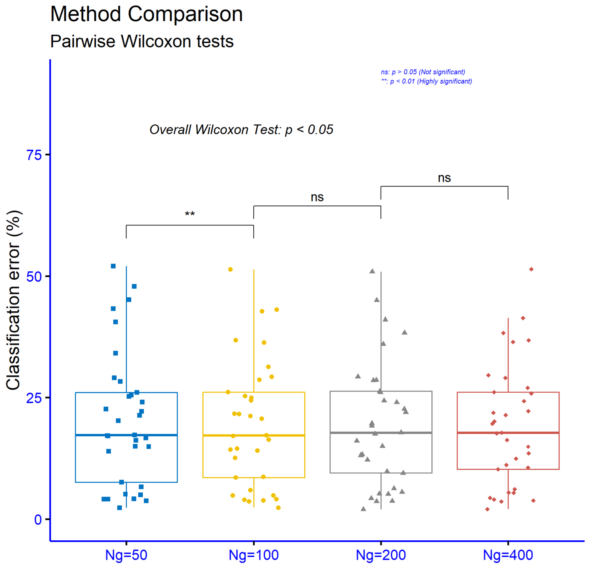
Figure 12 shows that increasing the number of generations from $N_g=50$ to $N_g=100$ yields a statistically significant improvement ($p<0.01$, **), indicating a meaningful reduction in error in this range. By contrast, the comparisons $N_g=100$ vs. $N_g=200$ and $N_g=200$ vs. $N_g=400$ are not statistically significant ($p>0.05$, ns), which means that further increasing generations beyond 100 does not produce a consistent additional gain in performance. Overall, the results suggest that the main benefit is achieved early up to about 100 generations, after which returns diminish and the differences are not statistically meaningful.

In Figure 13, the p-value analysis on the regression datasets shows that the comparison between $N_g=50$ and $N_g=100$ is not statistically significant ($p>0.05$, ns), so increasing generations in this range does not yield a consistent improvement. By contrast, moving from $N_g=100$ to $N_g=200$ is statistically significant ($p<0.05$, *), indicating a measurable reduction in error around 200 generations. Finally, the comparison between $N_g=200$ and $N_g=400$ is not statistically significant ($p>0.05$, ns), suggesting diminishing returns beyond 200 generations. Overall, the findings indicate that for regression problems the benefit concentrates around 200 generations, while further increases in $N_g$ do not guarantee additional consistent gains.

4.5. Experiments with Real-World Problems

A practical problem addressed in this context is the prediction of forest fire duration, which has been recently investigated for the Greek region [111]. An experiment was conducted using data from the Greek Fire Service to predict forest fire durations over the period 2014–2024. In this experiment, the following methods were used:

• A neural network with 10 computing nodes, trained using the BFGS optimizer.
• A radial basis function with 10 weights, trained with the original method for RBF training.
• The proposed method.

The results for the prediction of the duration are graphically illustrated in Figure 14. As is evident from the graph, in almost all years the classification error of the proposed technique is lower than that of the other two machine learning techniques.

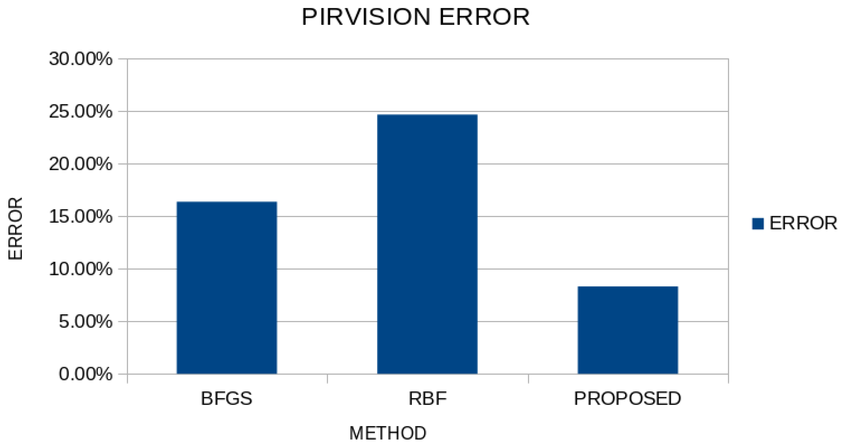
The second real-world example is the PIRvision dataset [112] with 15,302 patterns, with every pattern containing 59 features. The same machine learning models were also used in this case and the average classification error for these methods is depicted graphically in Figure 15. Again, the proposed method has a lower classification error than the other methods involved in this experiment.

5. Conclusions

The final experimental evidence shows that the three-phase RBF training pipeline, bound construction via K-means, global search with a GA inside those bounds, and local refinement with BFGS, yields robust gains across heterogeneous classification and regression tasks. On classification, it achieves the lowest mean error (19.45%), with extremely significant superiority over all baselines $\left(p<0.0001\right)$; on regression, it attains the smallest mean absolute error (5.87), with $p<0.01$ against BFGS/ADAM and $p<0.0001$ against NEAT/RBF-KMEANS/GENRBF. These results indicate that coupling broad exploration with constrained, precise local tuning mitigates numerical instability and local minima, providing reproducible performance improvements.

Sensitivity analyses reveal that the scale factor F materially affects classification in small-to-intermediate settings ($F=1\to 2$ and $F=2\to 4$ are significant at $p<0.01$), with no meaningful gain from $F=4$ to $F=8$, whereas for regression the F comparisons are not significant, highlighting methodological stability. Alternative $\sigma$ computation methods $\left({\sigma }_1,{\sigma }_{\mathrm{avg}},{\sigma }_{\max }\right)$ differ only marginally on average and show no significant differences in either task, reinforcing the method’s resilience to low-level design choices.

Automating architecture and hyperparameter adaptation is a natural next step. Joint optimization of the number of RBF units, F, and bounds via Bayesian optimization or meta-learning could reduce manual tuning and improve generalization. Exploring alternative global optimizers (e.g., DE, PSO, and CMA-ES) or hybrid GA and Bayesian strategies may accelerate convergence and enhance exploration, while in the final stage L-BFGS, bound-aware variants, and stochastic formulations could benefit large-scale, high-dimensional settings. A thorough ablation study to quantify each phase’s contribution, along with broader post hoc statistics, would strengthen the evidence base. From a systems perspective, parallel/distributed GA evaluations and GPU-accelerated RBF computations can materially cut runtime. Finally, extending benchmarks to strong non-RBF baselines and integrating the approach into AutoML pipelines together with analyses of interpretability and predictive uncertainty will provide a more complete picture of the method’s limits and potential.

It is important to note that, although highly effective, the proposed method is more computationally intensive than other machine learning approaches because of the sequential application of its three training stages. Specifically, the second stage, which applies the genetic algorithm, requires considerable computational effort. This overhead, however, can be mitigated by leveraging modern parallel computing techniques like OpenMP [113] or MPI [114].

References

1. Raissi, M.; Karniadakis, G.E. Hidden physics models: Machine learning of nonlinear partial differential equations. J. Comput. Phys. 2018, 357, 125–141. [Google Scholar] [CrossRef]
2. Kashinath, K.; Mustafa, M.; Albert, A.; Wu, J.-L.; Jiang, C.; Esmaeilzadeh, S.; Azizzadenesheli, K.; Wang, R.; Chattopadhyay, A.; Singh, A.; et al. Physics-informed machine learning: Case studies for weather and climate modelling. Philos. Trans. R. Soc. A 2021, 379, 20200093. [Google Scholar] [CrossRef]
3. Viquar, M.; Basak, S.; Dasgupta, A.; Agrawal, S.; Saha, S. Machine learning in astronomy: A case study in quasar-star classification. In Emerging Technologies in Data Mining and Information Security: Proceedings of IEMIS 2018; Springer: Singapore, 2019; Volume 3, pp. 827–836. [Google Scholar]
4. Luo, S.; Leung, A.P.; Hui, C.Y.; Li, K.L. An investigation on the factors affecting machine learning classifications in gamma-ray astronomy. Mon. Not. R. Astron. Soc. 2020, 492, 5377–5390. [Google Scholar] [CrossRef]
5. Meuwly, M. Machine learning for chemical reactions. Chem. Rev. 2021, 121, 10218–10239. [Google Scholar] [CrossRef]
6. Aguiar, J.A.; Gong, M.L.; Tasdizen, T. Crystallographic prediction from diffraction and chemistry data for higher throughput classification using machine learning. Comput. Mater. Sci. 2020, 173, 109409. [Google Scholar] [CrossRef]
7. Yadav, S.S.; Jadhav, S.M. Deep convolutional neural network based medical image classification for disease diagnosis. J. Big Data 2019, 6, 113. [Google Scholar] [CrossRef]
8. Qing, L.; Linhong, W.; Xuehai, D. A Novel Neural Network-Based Method for Medical Text Classification. Future Internet 2019, 11, 255. [Google Scholar] [CrossRef]
9. Athey, S. The impact of machine learning on economics. In The Economics of Artificial Intelligence: An Agenda; University of Chicago Press: Chicago, IL, USA, 2018; pp. 507–547. [Google Scholar]
10. Hafezi, R.; Shahrabi, J.; Hadavandi, E. A bat-neural network multi-agent system (BNNMAS) for stock price prediction: Case study of DAX stock price. Appl. Soft Comput. 2015, 29, 196–210. [Google Scholar] [CrossRef]
11. Ghai, D.; Tripathi, S.L.; Saxena, S.; Chanda, M.; Alazab, M. (Eds.) Machine Learning Algorithms for Signal and Image Processing; John Wiley & Sons: Hoboken, NJ, USA, 2022. [Google Scholar]
12. Ahmed, N.K.; Atiya, A.F.; Gayar, N.E.; El-Shishiny, H. An empirical comparison of machine learning models for time series forecasting. Econom. Rev. 2010, 29, 594–621. [Google Scholar] [CrossRef]
13. Radha, V.; Nallammal, N. Neural network based face recognition using RBFN classifier. In Proceedings of the World Congress on Engineering and Computer Science, San Francisco, CA, USA, 19–21 October 2011; Volume 1, pp. 19–21. [Google Scholar]
14. Kumar, M.; Yadav, N. Multilayer perceptrons and radial basis function neural network methods for the solution of differential equations: A survey. Comput. Math. Appl. 2011, 62, 3796–3811. [Google Scholar] [CrossRef]
15. Zhang, Y. An accurate and stable RBF method for solving partial differential equations. Appl. Math. Lett. 2019, 97, 93–98. [Google Scholar] [CrossRef]
16. Dash, R.; Dash, P.K. A comparative study of radial basis function network with different basis functions for stock trend prediction. In Proceedings of the 2015 IEEE Power, Communication and Information Technology Conference (PCITC), Bhubaneswar, India, 15–17 October 2015; IEEE: New York, NY, USA, 2015; pp. 430–435. [Google Scholar]
17. Lian, R.-J. Adaptive Self-Organizing Fuzzy Sliding-Mode Radial Basis-Function Neural-Network Controller for Robotic Systems. IEEE Trans. Ind. Electron. 2014, 61, 1493–1503. [Google Scholar] [CrossRef]
18. Vijay, M.; Jena, D. Backstepping terminal sliding mode control of robot manipulator using radial basis functional neural networks. Comput. Electr. Eng. 2018, 67, 690–707. [Google Scholar] [CrossRef]
19. Ravale, U.; Marathe, N.; Padiya, P. Feature Selection Based Hybrid Anomaly Intrusion Detection System Using K Means and RBF Kernel Function. Procedia Comput. Sci. 2015, 45, 428–435. [Google Scholar] [CrossRef]
20. Lopez-Martin, M.; Sanchez-Esguevillas, A.; Arribas, J.I.; Carro, B. Network Intrusion Detection Based on Extended RBF Neural Network With Offline Reinforcement Learning. IEEE Access 2021, 9, 153153–153170. [Google Scholar] [CrossRef]
21. Leonard, J.A.; Kramer, M.A. Radial basis function networks for classifying process faults. IEEE Control Syst. Mag. 1991, 11, 31–38. [Google Scholar] [CrossRef]
22. Gan, M.; Peng, H.; Dong, X.P. A hybrid algorithm to optimize RBF network architecture and parameters for nonlinear time series prediction. Appl. Math. Model. 2012, 36, 2911–2919. [Google Scholar] [CrossRef]
23. Sideratos, G.; Hatziargyriou, N. Using Radial Basis Neural Networks to Estimate Wind Power Production. In Proceedings of the 2007 IEEE Power Engineering Society General Meeting, Tampa, FL, USA, 24–28 June 2007; pp. 1–7. [Google Scholar] [CrossRef]
24. Park, J.; Sandberg, I.W. Universal Approximation Using Radial-Basis-Function Networks. Neural Comput. 1991, 3, 246–257. [Google Scholar] [CrossRef]
25. MacQueen, J. Some methods for classification and analysis of multivariate observations. In Proceedings of the Fifth Berkeley Symposium on Mathematical Statistics and Probability, Los Angeles, CA, USA, 21 June–18 July 1965, 27 December 1965–7 January 1966; Volume 1, pp. 281–297. [Google Scholar]
26. Kuncheva, L.I. Initializing of an RBF network by a genetic algorithm. Neurocomputing 1997, 14, 273–288. [Google Scholar] [CrossRef]
27. Ros, F.; Pintore, M.; Deman, A.; Chrétien, J.R. Automatical initialization of RBF neural networks. Chemom. Intell. Lab. Syst. 2007, 87, 26–32. [Google Scholar] [CrossRef]
28. Wang, D.; Zeng, X.J.; Keane, J.A. A clustering algorithm for radial basis function neural network initialization. Neurocomputing 2012, 77, 144–155. [Google Scholar] [CrossRef]
29. Benoudjit, N.; Verleysen, M. On the Kernel Widths in Radial-Basis Function Networks. Neural Process. Lett. 2003, 18, 139–154. [Google Scholar] [CrossRef]
30. Määttä, J.; Bazaliy, V.; Kimari, J.; Djurabekova, F.; Nordlund, K.; Roos, T. Gradient-based training and pruning of radial basis function networks with an application in materials physics. Neural Netw. 2021, 133, 123–131. [Google Scholar] [CrossRef]
31. Gale, S.; Vestheim, S.; Gravdahl, J.T.; Fjerdingen, S.; Schjølberg, I. RBF network pruning techniques for adaptive learning controllers. In Proceedings of the 9th International Workshop on Robot Motion and Control, Kuslin, Poland, 3–5 July 2013; IEEE: New York, NY, USA, 2013; pp. 246–251. [Google Scholar]
32. Bortman, M.; Aladjem, M. A Growing and Pruning Method for Radial Basis Function Networks. IEEE Trans. Neural Netw. 2009, 20, 1039–1045. [Google Scholar] [CrossRef]
33. Du, J.X.; Huang, D.S.; Zhang, G.J.; Wang, Z.F. A novel full structure optimization algorithm for radial basis probabilistic neural networks. Neurocomputing 2006, 70, 592–596. [Google Scholar] [CrossRef]
34. Yu, H.; Reiner, P.D.; Xie, T.; Bartczak, T.; Wilamowski, B.M. An incremental design of radial basis function networks. IEEE Trans. Neural Netw. Learn. Syst. 2014, 25, 1793–1803. [Google Scholar] [CrossRef]
35. Jia, W.; Zhao, D.; Ding, L. An optimized RBF neural network algorithm based on partial least squares and genetic algorithm for classification of small sample. Appl. Soft Comput. 2016, 48, 373–384. [Google Scholar] [CrossRef]
36. Zhang, W.; Wei, D. Prediction for network traffic of radial basis function neural network model based on improved particle swarm optimization algorithm. Neural Comput. Appl. 2018, 29, 1143–1152. [Google Scholar] [CrossRef]
37. Qasem, S.N.; Shamsuddin, S.M.; Zain, A.M. Multi-objective hybrid evolutionary algorithms for radial basis function neural network design. Knowl.-Based Syst. 2012, 27, 475–497. [Google Scholar] [CrossRef]
38. Yokota, R.; Barba, L.A.; Knepley, M.G. PetRBF—A parallel O(N) algorithm for radial basis function interpolation with Gaussians. Comput. Methods Appl. Mech. Eng. 2010, 199, 1793–1804. [Google Scholar] [CrossRef]
39. Lu, C.; Ma, N.; Wang, Z. Fault detection for hydraulic pump based on chaotic parallel RBF network. EURASIP J. Adv. Signal Process. 2011, 2011, 49. [Google Scholar] [CrossRef]
40. Rani, R.H.J.; Victoire, T.A.A. Training radial basis function networks for wind speed prediction using PSO enhanced differential search optimizer. PLoS ONE 2018, 13, e0196871. [Google Scholar] [CrossRef] [PubMed]
41. Karamichailidou, D.; Gerolymatos, G.; Patrinos, P.; Sarimveis, H.; Alexandridis, A. Radial basis function neural network training using variable projection and fuzzy means. Neural Comput. Appl. 2024, 36, 21137–21151. [Google Scholar] [CrossRef]
42. Krishna, K.; Narasimha, M. Murty, Genetic K-means algorithm. IEEE Trans. Syst. Man Cybern. Part B (Cybern.) 1999, 29, 433–439. [Google Scholar] [CrossRef]
43. Sinaga, K.P.; Yang, M.-S. Unsupervised K-Means Clustering Algorithm. IEEE Access 2020, 8, 80716–80727. [Google Scholar] [CrossRef]
44. Ay, M.; Özbakır, L.; Kulluk, S.; Gülmez, B.; Öztürk, G.; Özer, S. FC-Kmeans: Fixed-centered K-means algorithm. Expert Syst. Appl. 2023, 211, 118656. [Google Scholar] [CrossRef]
45. Oti, E.U.; Olusola, M.O.; Eze, F.C.; Enogwe, S.U. Comprehensive review of K-Means clustering algorithms. Criterion 2021, 12, 22–23. [Google Scholar] [CrossRef]
46. Grady, S.A.; Hussaini, M.Y.; Abdullah, M.M. Placement of wind turbines using genetic algorithms. Renew. Energy 2005, 30, 259–270. [Google Scholar] [CrossRef]
47. Parvaze, S.; Kumar, R.; Khan, J.N.; Al-Ansari, N.; Parvaze, S.; Vishwakarma, D.K.; Elbeltagi, A.; Kuriqi, A. Optimization of water distribution systems using genetic algorithms: A review. Arch. Comput. Methods Eng. 2023, 30, 4209–4244. [Google Scholar] [CrossRef]
48. Gordini, N. A genetic algorithm approach for SMEs bankruptcy prediction: Empirical evidence from Italy. Expert Syst. Appl. 2014, 41, 6433–6445. [Google Scholar] [CrossRef]
49. Ding, S.; Su, C.; Yu, J. An optimizing BP neural network algorithm based on genetic algorithm. Artif. Intell. Rev. 2011, 36, 153–162. [Google Scholar] [CrossRef]
50. Guo, L.; Funie, A.I.; Thomas, D.B.; Fu, H.; Luk, W. Parallel genetic algorithms on multiple FPGAs. ACM SIGARCH Comput. Archit. News 2016, 43, 86–93. [Google Scholar] [CrossRef]
51. Johar, F.M.; Azmin, F.A.; Suaidi, M.K.; Shibghatullah, A.S.; Ahmad, B.H.; Salleh, S.N.; Abidin Abd Aziz, M.Z.; Shukor, M.M. A review of genetic algorithms and parallel genetic algorithms on graphics processing unit (GPU). In Proceedings of the 2013 IEEE International Conference on Control System, Computing and Engineering, Penang, Malaysia, 29 November–1 December 2013; IEEE: New York, NY, USA, 2013; pp. 264–269. [Google Scholar]
52. Kaelo, P.; Ali, M.M. Integrated crossover rules in real coded genetic algorithms. Eur. J. Oper. Res. 2007, 176, 60–76. [Google Scholar] [CrossRef]
53. Powell, M.J.D. A Tolerant Algorithm for Linearly Constrained Optimization Calculations. Math. Program. 1989, 45, 547–566. [Google Scholar] [CrossRef]
54. Liu, D.C.; Nocedal, J. On the limited memory BFGS method for large scale optimization. Math. Program. 1989, 45, 503–528. [Google Scholar] [CrossRef]
55. Mokhtari, A.; Ribeiro, A. RES: Regularized Stochastic BFGS Algorithm. IEEE Trans. Signal Process. 2014, 62, 6089–6104. [Google Scholar] [CrossRef]
56. Dai, Y.H. Convergence properties of the BFGS algoritm. SIAM J. Optim. 2002, 13, 693–701. [Google Scholar] [CrossRef]
57. Kelly, M.; Longjohn, R.; Nottingham, K. The UCI Machine Learning Repository. Available online: https://archive.ics.uci.edu (accessed on 28 September 2025).
58. Alcalá-Fdez, J.; Fernandez, A.; Luengo, J.; Derrac, J.; Sánchez, L.; Herrera, F. KEEL Data-Mining Software Tool: Data Set Repository, Integration of Algorithms and Experimental Analysis Framework. J. Mult.-Valued Log. Soft Comput. 2011, 17, 255–287. [Google Scholar]
59. Kooperberg, C. Statlib: An archive for statistical software, datasets, and information. Am. Stat. 1997, 51, 98. [Google Scholar] [CrossRef]
60. Weiss, S.M.; Kulikowski, C.A. Computer Systems That Learn: Classification and Prediction Methods from Statistics, Neural Nets, Machine Learning, and Expert Systems; Morgan Kaufmann Publishers Inc.: Burlington, MA, USA, 1991. [Google Scholar]
61. Tzimourta, K.D.; Tsoulos, I.; Bilero, I.T.; Tzallas, A.T.; Tsipouras, M.G.; Giannakeas, N. Direct Assessment of Alcohol Consumption in Mental State Using Brain Computer Interfaces and Grammatical Evolution. Inventions 2018, 3, 51. [Google Scholar] [CrossRef]
62. Quinlan, J.R. Simplifying Decision Trees. Int. J. Man-Mach. Stud. 1987, 27, 221–234. [Google Scholar] [CrossRef]
63. Shultz, T.; Mareschal, D.; Schmidt, W. Modeling Cognitive Development on Balance Scale Phenomena. Mach. Learn. 1994, 16, 59–88. [Google Scholar] [CrossRef]
64. Zhou, Z.H.; Jiang, Y. NeC4.5: Neural ensemble based C4.5. IEEE Trans. Knowl. Data Eng. 2004, 16, 770–773. [Google Scholar] [CrossRef]
65. Setiono, R.; Leow, W.K. FERNN: An Algorithm for Fast Extraction of Rules from Neural Networks. Appl. Intell. 2000, 12, 15–25. [Google Scholar] [CrossRef]
66. Gavrilis, D.; Tsoulos, I.G.; Dermatas, E. Selecting and constructing features using grammatical evolution. Pattern Recognit. Lett. 2008, 29, 1358–1365. [Google Scholar] [CrossRef]
67. Demiroz, G.; Govenir, H.A.; Ilter, N. Learning Differential Diagnosis of Eryhemato-Squamous Diseases using Voting Feature Intervals. Artif. Intell. Med. 1998, 13, 147–165. [Google Scholar]
68. Horton, P.; Nakai, K. A Probabilistic Classification System for Predicting the Cellular Localization Sites of Proteins. Proc. Int. Conf. Intell. Syst. Mol. Biol. 1996, 4, 109–115. [Google Scholar]
69. Hayes-Roth, B.; Hayes-Roth, F. Concept learning and the recognition and classification of exemplars. J. Verbal Learn. Verbal Behav. 1977, 16, 321–338. [Google Scholar] [CrossRef]
70. Kononenko, I.; Šimec, E.; Robnik-Šikonja, M. Overcoming the Myopia of Inductive Learning Algorithms with RELIEFF. Appl. Intell. 1997, 7, 39–55. [Google Scholar] [CrossRef]
71. Rashid, T.A.; Bryar, H. Heart Attack Dataset. Mendeley Data 2022, V1. [Google Scholar] [CrossRef]
72. French, R.M.; Chater, N. Using noise to compute error surfaces in connectionist networks: A novel means of reducing catastrophic forgetting. Neural Comput. 2002, 14, 1755–1769. [Google Scholar] [CrossRef] [PubMed]
73. Dy, J.G.; Brodley, C.E. Feature Selection for Unsupervised Learning. J. Mach. Learn. Res. 2004, 5, 845–889. [Google Scholar]
74. Perantonis, S.J.; Virvilis, V. Input Feature Extraction for Multilayered Perceptrons Using Supervised Principal Component Analysis. Neural Process. Lett. 1999, 10, 243–252. [Google Scholar] [CrossRef]
75. Garcke, J.; Griebel, M. Classification with sparse grids using simplicial basis functions. Intell. Data Anal. 2002, 6, 483–502. [Google Scholar] [CrossRef]
76. Mcdermott, J.; Forsyth, R.S. Diagnosing a disorder in a classification benchmark. Pattern Recognit. Lett. 2016, 73, 41–43. [Google Scholar] [CrossRef]
77. Cestnik, G.; Konenenko, I.; Bratko, I. Assistant-86: A Knowledge-Elicitation Tool for Sophisticated Users. In Progress in Machine Learning; Bratko, I., Lavrac, N., Eds.; Sigma Press: Wilmslow, UK, 1987; pp. 31–45. [Google Scholar]
78. Elter, M.; Schulz-Wendtland, R.; Wittenberg, T. The prediction of breast cancer biopsy outcomes using two CAD approaches that both emphasize an intelligible decision process. Med. Phys. 2007, 34, 4164–4172. [Google Scholar] [CrossRef]
79. Little, M.A.; McSharry, P.E.; Hunter, E.J.; Spielman, J.; Ramig, L.O. Suitability of dysphonia measurements for telemonitoring of Parkinson’s disease. IEEE Trans Biomed Eng. 2009, 56, 1015–1022. [Google Scholar] [CrossRef]
80. Smith, J.W.; Everhart, J.E.; Dickson, W.C.; Knowler, W.C.; Johannes, R.S. Using the ADAP learning algorithm to forecast the onset of diabetes mellitus. In Proceedings of the Annual Symposium on Computer Application in Medical Care, Washington, DC, USA, 6–9 November 1988; IEEE Computer Society Press: New York, NY, USA, 1988; pp. 261–265. [Google Scholar]
81. Lucas, D.D.; Klein, R.; Tannahill, J.; Ivanova, D.; Brandon, S.; Domyancic, D.; Zhang, Y. Failure analysis of parameter-induced simulation crashes in climate models. Geosci. Model Dev. 2013, 6, 1157–1171. [Google Scholar] [CrossRef]
82. Giannakeas, N.; Tsipouras, M.G.; Tzallas, A.T.; Kyriakidi, K.; Tsianou, Z.E.; Manousou, P.; Hall, A.; Karvounis, E.C.; Tsianos, V.; Tsianos, E. A clustering based method for collagen proportional area extraction in liver biopsy images. In Proceedings of the Annual International Conference of the IEEE Engineering in Medicine and Biology Society, EMBS, Milan, Italy, 25–29 August 2015; pp. 3097–3100. [Google Scholar]
83. Hastie, T.; Tibshirani, R. Non-parametric logistic and proportional odds regression. J. R. Stat. Soc. Ser. C (Appl. Stat.) 1987, 36, 260–276. [Google Scholar] [CrossRef]
84. Dash, M.; Liu, H.; Scheuermann, P.; Tan, K.L. Fast hierarchical clustering and its validation. Data Knowl. Eng. 2003, 44, 109–138. [Google Scholar] [CrossRef]
85. Dua, D.; Graff, C. UCI Machine Learning Repository; University of California, School of Information and Computer Science: Irvine, CA, USA, 2019; Available online: http://archive.ics.uci.edu/ml (accessed on 29 October 2025).
86. Cortez, P.; Silva, A.M.G. Using data mining to predict secondary school student performance. In Proceedings of the 5th FUture BUsiness TEChnology Conference (FUBUTEC 2008), Porto, Portugal, 9–11 April 2008; pp. 5–12. [Google Scholar]
87. Yeh, I.-C.; Yang, K.-J.; Ting, T.-M. Knowledge discovery on RFM model using Bernoulli sequence. Expert Syst. Appl. 2009, 36, 5866–5871. [Google Scholar] [CrossRef]
88. Jeyasingh, S.; Veluchamy, M. Modified bat algorithm for feature selection with the Wisconsin diagnosis breast cancer (WDBC) dataset. Asian Pac. J. Cancer Prev. APJCP 2017, 18, 1257. [Google Scholar]
89. Alshayeji, M.H.; Ellethy, H.; Gupta, R. Computer-aided detection of breast cancer on the Wisconsin dataset: An artificial neural networks approach. Biomed. Signal Process. Control 2022, 71, 103141. [Google Scholar] [CrossRef]
90. Raymer, M.; Doom, T.E.; Kuhn, L.A.; Punch, W.F. Knowledge discovery in medical and biological datasets using a hybrid Bayes classifier/evolutionary algorithm. IEEE Trans. Syst. Man Cybern. Part B Cybern. 2003, 33, 802–813. [Google Scholar] [CrossRef] [PubMed]
91. Zhong, P.; Fukushima, M. Regularized nonsmooth Newton method for multi-class support vector machines. Optim. Methods Softw. 2007, 22, 225–236. [Google Scholar] [CrossRef]
92. Andrzejak, R.G.; Lehnertz, K.; Mormann, F.; Rieke, C.; David, P.; Elger, C.E. Indications of nonlinear deterministic and finite-dimensional structures in time series of brain electrical activity: Dependence on recording region and brain state. Phys. Rev. E 2001, 64, 061907. [Google Scholar] [CrossRef]
93. Tzallas, A.T.; Tsipouras, M.G.; Fotiadis, D.I. Automatic Seizure Detection Based on Time-Frequency Analysis and Artificial Neural Networks. Comput. Intell. Neurosci. 2007, 2007, 80510. [Google Scholar] [CrossRef]
94. Koivisto, M.; Sood, K. Exact Bayesian Structure Discovery in Bayesian Networks. J. Mach. Learn. Res. 2004, 5, 549–573. [Google Scholar]
95. Nash, W.J.; Sellers, T.L.; Talbot, S.R.; Cawthor, A.J.; Ford, W.B. The Population Biology of Abalone (Haliotis species) in Tasmania. I. Blacklip Abalone (H. rubra) from the North Coast and Islands of Bass Strait, Sea Fisheries Division; Technical Report No. 48; Department of Primary Industry and Fisheries, Tasmania: Hobart, Australia, 1994; ISSN 1034–3288. [Google Scholar]
96. Brooks, T.F.; Pope, D.S.; Marcolini, A.M. Airfoil Self-Noise and Prediction. Technical Report, NASA RP-1218. July 1989. Available online: https://ntrs.nasa.gov/citations/19890016302 (accessed on 14 November 2024).
97. Quinlan, R. Combining Instance-Based and Model-Based Learning. In Proceedings of the Tenth International Conference of Machine Learning, Amherst, MA, USA, 27–29 June 1993; pp. 236–243. [Google Scholar]
98. Cheng Yeh, I. Modeling of strength of high performance concrete using artificial neural networks. Cem. Concr. Res. 1998, 28, 1797–1808. [Google Scholar] [CrossRef]
99. Friedman, J. Multivariate Adaptative Regression Splines. Ann. Stat. 1991, 19, 1–141. [Google Scholar]
100. Harrison, D.; Rubinfeld, D.L. Hedonic prices and the demand for clean ai. J. Environ. Econ. Manag. 1978, 5, 81–102. [Google Scholar] [CrossRef]
101. Tsoulos, I.G.; Charilogis, V.; Kyrou, G.; Stavrou, V.N.; Tzallas, A. OPTIMUS: A Multidimensional Global Optimization Package. J. Open Source Softw. 2025, 10, 7584. [Google Scholar] [CrossRef]
102. Yuan, Y.X. A modified BFGS algorithm for unconstrained optimization. IMA J. Numer. Anal. 1991, 11, 325–332. [Google Scholar] [CrossRef]
103. Bishop, C. Neural Networks for Pattern Recognition; Oxford University Press: Oxford, UK, 1995. [Google Scholar]
104. Cybenko, G. Approximation by superpositions of a sigmoidal function. Math. Control Signals Syst. 1989, 2, 303–314. [Google Scholar] [CrossRef]
105. Kingma, D.P.; Ba, J.L. ADAM: A method for stochastic optimization. In Proceedings of the 3rd International Conference on Learning Representations (ICLR 2015), San Diego, CA, USA, 7–9 May 2015; pp. 1–15. [Google Scholar]
106. Xue, Y.; Tong, Y.; Neri, F. An ensemble of differential evolution and Adam for training feed-forward neural networks. Inf. Sci. 2022, 608, 453–471. [Google Scholar] [CrossRef]
107. Stanley, K.O.; Miikkulainen, R. Evolving Neural Networks through Augmenting Topologies. Evol. Comput. 2002, 10, 99–127. [Google Scholar] [CrossRef]
108. Ward, R.; Wu, X.; Bottou, L. Adagrad stepsizes: Sharp convergence over nonconvex landscapes. J. Mach. Learn. Res. 2020, 21, 1–30. [Google Scholar]
109. Martinez-Cantin, R. BayesOpt: A Bayesian Optimization Library for Nonlinear Optimization, Experimental Design and Bandits. J. Mach. Learn. Res. 2014, 15, 3735–3739. [Google Scholar]
110. Ding, S.; Xu, L.; Su, C.; Jin, F. An optimizing method of RBF neural network based on genetic algorithm. Neural Comput. Appl. 2012, 21, 333–336. [Google Scholar] [CrossRef]
111. Kopitsa, C.; Tsoulos, I.G.; Charilogis, V.; Stavrakoudis, A. Predicting the Duration of Forest Fires Using Machine Learning Methods. Future Internet 2024, 16, 396. [Google Scholar] [CrossRef]
112. Emad-Ud-Din, M.; Wang, Y. Promoting occupancy detection accuracy using on-device lifelong learning. IEEE Sens. J. 2023, 23, 9595–9606. [Google Scholar] [CrossRef]
113. Saxena, R.; Jain, M.; Malhotra, K.; Vasa, K.D. An optimized openmp-based genetic algorithm solution to vehicle routing problem. In Smart Computing Paradigms: New Progresses and Challenges: Proceedings of ICACNI 2018; Springer: Singapore, 2019; Volume 2, pp. 237–245. [Google Scholar]
114. Rajan, S.D.; Nguyen, D.T. Design optimization of discrete structural systems using MPI-enabled genetic algorithm. Struct. Multidiscip. Optim. 2004, 28, 340–348. [Google Scholar] [CrossRef]
Figure 1. This figure depicts the Gaussian function with σ = 1 and c = 0 .
Ai 06 00280 g001
Figure 2. A graphical presentation of the K-means algorithm.
Ai 06 00280 g002
Figure 3. The bound construction algorithm.
Ai 06 00280 g003
Figure 4. The figure illustrates the schematic arrangement of a chromosome in the proposed genetic algorithm.
Ai 06 00280 g004
Figure 5. Summary flowchart of the proposed method.
Ai 06 00280 g005
Figure 6. Statistical analyses of the results obtained on the classification datasets with the machine learning methods discussed in this work.
Ai 06 00280 g006
Figure 7. Statistical analysis comparing the results produced by the set of machine learning methods applied to the regression datasets.
Ai 06 00280 g007
Figure 8. Statistical evaluation of the outcomes produced by the proposed approach on the classification datasets, considering variations in the parameter F.
Ai 06 00280 g008
Figure 9. Statistical evaluation of the outcomes produced by the proposed approach on the regression datasets, with variations in the parameter F.
Ai 06 00280 g009
Figure 10. Statistical evaluation of the outcomes from applying the proposed method to the classification datasets, considering various approaches for determining the range of σ parameters in the radial basis functions.
Ai 06 00280 g010
Figure 11. Statistical analysis of the outcomes from applying the current method to the regression datasets, considering different approaches for determining the range of σ parameters in the radial functions.
Ai 06 00280 g011
Figure 12. Statistical evaluation of the outcomes from applying the proposed method to the classification datasets, with different settings of the parameter N g .
Ai 06 00280 g012
Figure 13. Statistical evaluation of the outcomes from applying the proposed method to the regression datasets, with different settings of the parameter N g .
Ai 06 00280 g013
Figure 14. Average classification error for the years 2014-2023 for forest fires in the Greek territory.
Ai 06 00280 g014
Figure 15. The experimental results for the PIRvision dataset.
Ai 06 00280 g015