An AutoML Algorithm: Multiple-Steps Ahead Forecasting of Correlated Multivariate Time Series with Anomalies Using Gated Recurrent Unit Networks

Abstract

Multiple time series forecasting is critical in domains such as energy management, economic analysis, web traffic prediction and air pollution monitoring to support effective resource planning. Traditional statistical learning methods, including Vector Autoregression (VAR) and Vector Autoregressive Integrated Moving Average (VARIMA), struggle with nonstationarity, temporal dependencies, inter-series correlations, and data anomalies such as trend shifts, seasonal variations, and missing data. Furthermore, their effectiveness in multi-step ahead forecasting is often limited. This article presents an Automated Machine Learning (AutoML) framework that provides an end-to-end solution for researchers who lack in-depth knowledge of time series forecasting or advanced programming skills. This framework utilizes Gated Recurrent Unit (GRU) networks, a variant of Recurrent Neural Networks (RNNs), to tackle multiple correlated time series forecasting problems, even in the presence of anomalies. To reduce complexity and facilitate the AutoML process, many model parameters are pre-specified, thereby requiring minimal tuning. This design enables efficient and accurate multi-step forecasting while addressing issues including missing values and structural shifts. We also examine the advantages and limitations of GRU-based RNNs within the AutoML system for multivariate time series forecasting. Model performance is evaluated using multiple accuracy metrics across various forecast horizons. The empirical results confirm our proposed approach’s ability to capture inter-series dependencies and handle anomalies in long-range forecasts.

1. Introduction

Time series forecasting has received attention across a great number of research disciplines for decades, such as power energy [1], economy [2], web traffic [3] and air pollution [4]. At present, most real-world data usually exhibit multivariate time series characteristics: seasonality, trends, and correlation among multivariate time series. Because of the arrival of the digital generation, multivariate time-series data and their complexity have been massively increased. Major challenges in real-world multivariate time series forecasting tasks are: (1) long-term dependency, (2) inter-series correlations, (3) nonlinearity and shifted trends, (4) gaps or missing values in the time series, and (5) the increasing complexity and dimensionality of time series data.

Despite the broad applications of statistical and ML-based methods, handling multivariate time-series forecasting tasks requires professional expertise in data science and statistics, significant time costs, and substantial manual involvements. VAR and VARIMA [5,6] are classical statistical models designed primarily for multivariate time series. A VAR model expresses each variable being considered and a serially uncorrelated error term [7]. VARIMA extends VAR by adding moving average (MA) components and incorporating differencing, allowing it to capture both short- and long-term dynamics in the data. However, ML-based and AutoML-based models can automatically capture nonlinear patterns without requiring time series assumptions such as stationarity. AutoML [8] is critically important as it aims to provide an end-to-end automated solution for non-professionals in time series forecasting. The goal of AutoML is to use raw data as the input to produce a high-quality model efficiently and output with minimal human intervention [9, 10, 11,12]. In addition, these models can be retrained periodically to reflect any changes in the data and maintain high-quality performance efficiently. An AutoML system has three attributes: full automation, adaptability, and high-quality [9,10,12]. AutoML approaches are designed for a specialized search space for time series models, including convolution, recurrent, gating units, etc. [12]. Moreover, their search spaces consist of core hyperparameters, activation functions and optimizers, and AutoML frameworks can systematically suggest the optimal configurations of those components. To increase robustness of time-series models, the AutoML system assembles the top suitable models and generates the best combination of hyperparameters discovered in the search space. In our proposed method, time series predictions are produced in the way of recursive or multiple-steps ahead forecasting.

Our previous study [9] has empirically shown that the overall performance of LSTM networks in univariate time series forecasts outperform that of classical statistical methods and other neural networks (NNs) within the AutoML framework, by practicing AutoML attributes and obtaining the highest forecasting accuracy in every length. The extended study [10] proposes using an LSTM network within an AutoML framework to perform the short- and long-term forecasting of correlated bivariate time series, even when the inter-series correlation is small. Empirical evidence further suggests that forecasting both time series jointly yields lower prediction errors compared to modeling each time series independently. Incorporating inter-series correlation as a contributing factor, we have found that higher correlations between time series generally lead to better forecasting performance. Despite low inter-series correlations, jointly analyzing correlated time series can still enhance forecasting accuracy. This research focuses on developing an AutoML framework that allows users to leverage multiple inter-correlated time series with data anomalies including trend shifts and the presence of missing values across multiple series to perform both short-term and long-term forecasting effectively. The proposed method employs GRU networks to perform multi-step ahead forecasting, while ensuring minimal human intervention and the automatic adaptability of new data, achieved through pre-specified hyperparameter tuning and fewer selective DL models. In the simulation, inter-series correlations are introduced using Lower–Upper (LU) Decomposition [13]. We then simulate trend shifts and missing values to assess the proposed model’s robustness. Furthermore, we emphasize the practical implications of our AutoML approach and its effectiveness in real-world scenarios. A real dataset is used to validate our findings.

Our research hypotheses include: the higher the inter-series correlation among multiple series, the better the forecasting performances; and time-series data anomalies cause higher forecasting errors. The main contributions of our article are summarized as follows:

(1)

By meeting the AutoML attributes, we provide a novel approach with minimal preprocessing to multiple-steps-ahead forecast correlated multivariate time series, while addressing the shiftiness of trends and missing values in the data.

(2)

Fixing multiple hyperparameters in the GRU-RNN model, the proposed approach can significantly speed up the training process without compromising predictive performance.

(3)

Empirical results are provided to investigate the experimental effects of previously mentioned components and to show that our proposed methods outperform traditional and AutoML-based methods.

(4)

To solve real-world forecasting tasks in the economic, financial and energy sectors, the proposed AutoML approach can reduce the technical barriers and facilitate broader adoption across interdisciplinary fields.

The remaining sections of this study proceed as follows. Section 2 discusses related research from two perspectives: statistical time series methods and recent ML-based methods. Section 3 discusses the theoretical aspects of traditional forecasting models and AutoML-based models and introduces their integration of the AutoML system. Section 4 introduces simulated data and real data and discusses the experimental designs. Section 5 presents a comparative analysis report and empirical findings. Section 6 provides discussions of the proposed method, concludes this article and summarizes and highlights our research outcomes. Lastly, Section 7 discusses potential future research directions.

2. Related Works

2.1. Statistical Learning Approaches

Autoregressive Integrated Moving Average (ARIMA) or Seasonal ARIMA [5] is a classical statistical model that productively predicts univariate time series and presents competitive forecasting accuracy, compared to some NN models [9]. Meanwhile, the ARIMA model requires stationary time series to ensure valid future predictions [11]. Thus, the decomposition of nonstationary time series is a crucial preprocessing step in order to remove seasonality and trend patterns before proceeding to ARIMA model. This stationarity requirement should be met for the other statistical learning models.

Other than VAR and VARIMA, the Vector Autoregressive Fractionally Integrated Moving Average (VARFIMA) model can address the long-memory behavior of multivariate time series by allowing for fractional differencing parameters [14]. While the structure of VARFIMA can increase computational complexity, statistical methods are inevitably prone to overfitting and high computational costs as multivariate time series take on more high-dimensional inputs and complex patterns [15].

2.2. Machine-Learning-Based Approaches

As machine learning (ML) thrives in various fields and industries, time series research continues making significant progresses. All time series forecasting methods assume that there exists an underlying relationship between past values and future values. Artificial neural network (ANN) and DL algorithms can outperform traditional models, by better estimating this underlying function when solving complex patterns [16]. The achievements of ANNs and DL algorithms are also recognized, because of their flexibility, generalization and competitive quality.

Multivariate Temporal Convolutional Network (M-TCN) [15] and Multivariate Time Series Forecasting Framework via a Temporal Attention-based Encoder-decoder Model (MTSMFF) [17] are the novel NN structures proposed based on state-of-art of deep learning (DL), in order to improve multivariate time series predictions and adaptively learn inter-series correlation. At the same time, both models require data preprocessing and some degree of human intervention.

3. Methods

This section briefly discusses the theoretical aspects of both traditional time series methods and AutoML-based time series forecasting methods. We primarily introduce the integration of the AutoML framework and examine how these methods address the challenges of multivariate time series.

3.1. Vector Autoregressive (VAR) and Vector Autoregressive Integrated Moving Average (VARIMA)

VAR is a macroeconometric framework developed to systematically model the dynamic interrelationships among multivariate time series variables [18]. A VAR model is an $n$-equation, $n$-variable linear model in which each variable is in turn explained by its own lagged values, plus the current and past values of the remaining $n-1$ variables [7]. VARIMA is an extension of VAR, by adding an MA component and differencing. Due to their ability to capture interdependencies and model flexibility, the VAR and VARIMA models are widely applied in financial and economic tasks.

A VAR$\left(p\right)$ model and a VARIMA($p,d,q$) are defined, respectively, in Equations (1) and (2):

$$\mathit{\Phi }\left(B\right)\left({\mathit{Z}}_t-\mathit{\mu }\right)={\mathit{a}}_t$$

(1)

$$\mathit{\Phi }\left(B\right){\left(1-B\right)}^d\left({\mathit{Z}}_t-\mathit{\mu }\right)=\mathit{\Theta }\left(B\right){\mathit{a}}_t$$

(2)

where order $p$ is the lagged value, ${\left(1-B\right)}^d$ is the differencing operator of order $d$, $\mathit{\Phi }\left(B\right)=\mathit{I}-{\mathit{\Phi }}_{1}B-{\mathit{\Phi }}_2{B}^2-\cdots -{\mathit{\Phi }}_p{B}^p$, ${\mathit{\Phi }}_i$ is a $k\times k$ parameter matrix, $\mathit{\Theta }\left(B\right)=\mathit{I}+{\mathit{\Theta }}_{1}B+{\mathit{\Theta }}_2{B}^2+\cdots +{\mathit{\Theta }}_q{B}^q$ and ${\mathit{a}}_t$ is a sequence of white noise with mean $\mathbf{0}$ and covariance matrix $\mathsf{\Sigma }$.

Before modeling by VAR and VARIMA, data are required to be stationary to avoid spurious prediction results. A stochastic process $\{X_t{\}}_{t=1}^{\infty }$ is stationary if its statistical properties are independent of time. Meanwhile, seasonality and trends are significant and common patterns in nonstationary time series. To address nonstationarity, deseasonalization and detrend (DSDT) is a crucial step for data preprocessing. The aim of time series decomposition is to decompose a nonstationary time series $\{X_t{\}}_{t=1}^{\infty }$ into nonstationary effects and a remaining component [19]. Because VAR and VARIMA rely on linearity assumptions, they are limited to capturing nonlinear dependencies. In addition, estimating parameters can be difficult, labor intensive and time consuming, particularly for high-dimensional data.

Training Details

It is required to verify time series stationarity by conducting Augmented Dickey Fuller (ADF) tests [20] with a level of significance $\alpha = 0.05$. To stabilize the systems, DSDT is implemented as a preprocessing step for the VAR$\left(p\right)$ and VARIMA$\left(p,d,q\right)$ models by differencing the series until stationarity has been reached.

The Akaike Information Criterion (AIC) and Bayesian Information Criterion (BIC) in Equations (3) and (4) are the metrics utilized to select the optimal combination of parameters $p,d,q$:

$$AIC = 2k - 2ln\left(L\right)$$

(3)

$$BIC=kln\left(n\right)-2ln\left(L\right)$$

(4)

where $k$ is the number of parameters, $n$ is the number of observations and $ln\left(L\right)$ is log-likelihood of the model. Both AIC and BIC penalize the likelihood of the model as $p$ increases. A grid search is conducted until both AIC and BIC reach reasonably low values, starting from $p,q=1$ to 12, $d=\mathrm{0,1},2$, and a maximum value of $p=12$ due to monthly data. Compared to DL-based models, computational efficiency is superior in VAR and VARIMA due to their linear structures.

3.2. Long Short-Term Memory (LSTM) Within the AutoML Framework

RNNs are better aligned to model sequential and temporal data, because there exists a recurrent network in the structure, which is to maintain memory and capture dependency in the temporal data. In AutoML-based forecasting methods, two effective RNN variants, LSTM and GRU, are elaborated upon and utilized for multivariate time series prediction [21,22,23,24,25].

Given an input vector $x=x_1,\dots ,x_T=X_t\left(\mathsf{\omega }\right)$, a standard RNN computes the hidden state $h=h_1,\dots ,h_T$, where $t=1,\dots ,T$:

$$h_t=g\left(W{x}_t+U{h}_{t-1}+b\right)$$

(5)

where $g$ is the element-wise activation function, and $W,U, b$ are the weight matrices and bias vector parameters. Equation (5) is considered as an intermediate memory cell, denoting ${\tilde{c}}_t$. Then, Equations (6)–(8) are set by adding ${\tilde{c}}_t$ to the value of the previous internal memory cell $c_{t-1}$, to produce the current value of memory cell $c_t$:

$$c_t=f_t⨀c_{t-1}+i_t⨀{\tilde{c}}_t$$

(6)

$${\tilde{c}}_t=g\left(W_c{x}_t+U_c{h}_{t-1}+b_c\right)$$

(7)

$$h_t=o_t⨀g\left(c_t\right)$$

(8)

where $i_t,f_t,o_t$ represent input, forget and output activation vectors, respectively, and $⨀$ is an element-wise multiplication. Their mathematical expressions are Equations (9)–(11):

$$i_t=\sigma \left(W_i{x}_t+U_i{h}_{t-1}+b_i\right)$$

(9)

$$f_t=\sigma \left(W_f{x}_t+U_f{h}_{t-1}+b_f\right)$$

(10)

$$o_t=\sigma \left(W_o{x}_t+U_o{h}_{t-1}+b_o\right)$$

(11)

where $\sigma$ is the sigmoid function. Therefore, LSTM networks can effectively capture seasonality, trend and aperiodic patterns at an early stage and carry them across long distances.

Integration of AutoML-LSTM and Training Details

To integrate LSTM networks into an AutoML system, the input, forget and output gates within each memory cell can process raw data input and update parameters by selectively discarding irrelevant information and retaining useful memory. Comparing with statistical learning methods, AutoML approaches do not require stationarity conditions and hand-crafted parameters.

Both LSTM and GRU networks are applied on the open-source software Keras and TensorFlow. It is optional to normalize the data from the AutoML aspect, but it is highly recommended because of reduced computational costs. Then, the normalized training set proceeds to TimeseriesGenerator() to transform the sequential data into batches of input–output pairs. It adapts the sliding window technique and controls the number of lagged values (n_input) and batch size. n_input is selected as 12, because the data are in monthly form. n_feature = {3} is selected based on the number of variables in the data.

To facilitate the AutoML system,

Table 1. Fixed hyperparameters.

Hyperparameter	Value
loss function	mse
activation	ReLU
optimizer	Adam
metric	mean_absolute_error
epochs	175

specifies the fixed and core hyperparameters, and

Table 2. Hyperparameters to be searched in AutoML-LSTM.

Hyperparameter	Value
Input_shape: n_input	{12, 24}
LSTM units	{64, 128, 256}
Dropout rate after LSTM	{None, 0.1, 0.2, 0.3, 0.4}
Insertion of MaxPooling1D	{Yes, No}
Dense_1	{16, 32, 64, 128}
Dense_2	{8, 16, 32}
Insertion of Dense_2	{Yes, No}
Dense_3	{8, 16, 32}

specifies the hyperparameters to be searched or tuned based on the nature of the data. The proposed AutoML methods intend to reduce the computational intensity and runtime by setting some fixed hyperparameters. Enforcing and testing these hyperparameter can help users develop an optimal and valid combination of NNs. As shown empirically in [11], the rectified linear unit (ReLU) activation function combined with the Adam optimizer achieved the lowest forecasting errors in time series predictions. On the Keras interface, LSTM(), Dense(), MaxPooling1D() and Dropout() are the layer choices. Due to the nature of time series, LSTM() captures patterns from autocorrelation, lagged relationships and interdependencies between variables. Dense() performs the linear combination of the inputs. MaxPooling1D() reduces the computational complexity by decreasing dimensionality. Dropout() mitigates overfitting by randomly dropping out units during training. After completing the construction, output layer is Dense(3), matching n_feature. For high-dimensional multivariate time series, additional Dense layers can increase the probability of patterns being captured.

3.3. Gated Recurrent Units (GRUs) Within the AutoML Framework

Similar to the architecture of the LSTM network and AutoML setting, GRU has shown promising forecasting performance in various ML-based tasks, because GRUs’ networks are simpler and more computational efficient, consisting of fewer gates (update and reset gates). GRU has gating units that modulate the flow of information inside the unit; however, without separate memory cells, it maintains the effect of LSTM [22,26]. 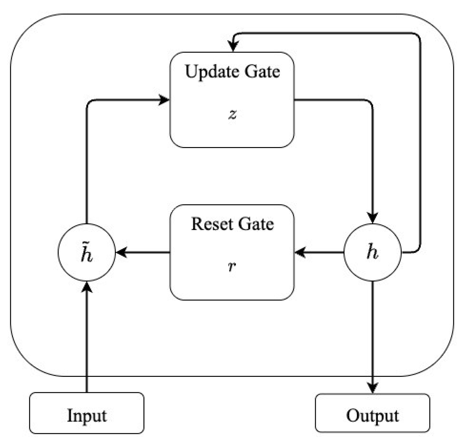Figure 1 presents the functioning of GRUs’ gates; $r, z$ are the reset and update gates, respectively.

At time $t$, the activation $h_t$ conducts a linear interpolation between a previous hidden state $h_{t-1}$ and the candidate activation ${\tilde{h}}_t$. The candidate activation ${\tilde{h}}_t$ computes in the similar way to the standard RNN in Equation (5). Mathematically, the GRU procedure is expressed as in Equations (12) and (13):

$$h_t=\left(1-z_t\right)⨀h_{t-1}+z_t⨀{\tilde{h}}_t$$

(12)

$${\tilde{h}}_t=g\left(W_h{x}_t+U_h\left(r_t⨀h_{t-1}\right)+b_h\right)$$

(13)

where the update and reset gate are Equations (14) and (15), respectively:

$$z_t=\sigma \left(W_z{x}_t+U_z{h}_{t-1}+b_z\right)$$

(14)

$$r_t=\sigma \left(W_r{x}_t+U_r{h}_{t-1}+b_r\right)$$

(15)

where $\sigma$ is the sigmoid function. The reset and update gates are calculated according to the previous hidden state $h_{t-1}$ and current input at time $t$. In the context of time series tasks, GRUs within the AutoML framework achieve lower computational costs while being able to effectively capture significant patterns.

Integration of AutoML-GRU and Training Details

The proposed AutoML-based methods can automatically and implicitly perform feature engineering inside their network structures. Similar to modeling AutoML-LSTM, Auto-GRU follows a comparable approach; thus, GRU() is operated on Keras to capture the temporal dependency of sequential data. Table 1 and

Table 3. Hyperparameters to be searched in AutoML-GRU.

Hyperparameter	Value
Input_shape: n_input	{12, 24}
GRU units	{64, 128, 256}
Dropout rate after GRU	{None, 0.1, 0.2, 0.3, 0.4}
Insertion of MaxPooling1D	{Yes, No}
Dense_1	{16, 32, 64, 128}
Dense_2	{8, 16, 32}
Insertion of Dense_2	{Yes, No}
Dense_3	{8, 16, 32}

are the hyperparameters being used and tested to construct the GRU model.

4. Experiments

Adapting a novel research design and extending the simulation from a previous study [10], this section first covers our proposed simulation of correlated multivariate time series with missing values and shifted trends. It also introduces the real data and presents the experimental settings of traditional and AutoML methods.

4.1. Simulation of Correlated Multivariate Time Series with Missing Values and Shifted Trends

An outline of our simulation is provided as follows.

(1)

Generate three independent time series, using the mixed decomposition model.

(2)

Generate shiftiness of trends on one selected simulated time series.

(3)

Given a correlation matrix with identical off-diagonal elements and perform LU decomposition on the matrix.

(4)

Using the decomposed lower triangular, transform uncorrelated time series to correlated multivariate time series.

(5)

Randomly generate missing values on one of the simulated multivariate time series, according to 15%, 10% and 5% missing values of the training set.

4.1.1. Independent Time Series

Our research focuses on monthly time series, as such data are commonly utilized and processed in economics and business. Both simulated and real data are structured in this form, due to the high granularity of the data and the better detection of data patterns. Adopting one of the research designs of [2], we choose the mixed decomposition model to generate independent time series. The mixed decomposition model introduces the nonstationary mean $\mu \left(t\right)$ and variance $\sigma \left(t\right)$ over time [19], because it involves both additive and multiplicative decompositions. To cope with seasonality and trend effects, three models are given in Equations (16)–(18):

$$x_t=T_t\times S{I1}_t+e_t$$

(16)

$$y_i=G_i\times SI{2}_i+e_i$$

(17)

$$s_j=K_j\times SI{3}_j+e_j$$

(18)

where, at time $t, i,j$, linear trend components are given by Equations (19)–(21), respectively, for each series:

$$T_i=100+0.6t$$

(19)

$$G_i=65+0.8i$$

(20)

$$K_j=150+1.1j$$

(21)

That is, $S{I1}_t$, $S{I2}_i$ and $SI{3}_j$ represent the seasonality indexes referred to

Table 4. Seasonal indexes for independent simulated time series.

Month	Jan	Feb	Mar	Apr	May	Jun
$SI1$	0.75	0.80	0.82	0.9	0.94	0.92
$SI2$	0.90	2	1.5	0.9	0.8	0.85
$SI3$	0.4	0.8	2	1.4	0.7	0.5
Month	Jul	Aug	Sept	Oct	Nov	Dec
$SI1$	0.91	0.99	0.95	1.02	1.2	1.8
$SI2$	1.7	0.8	0.6	1.87	1.2	1.9
$SI3$	0.68	1.5	0.35	1.98	2.2	1.6

, and $e_t,e_i,e_j$ are the Gaussian noise $N\left(0,{\sigma }^2\right)$ over time. $\sigma = 15$ is selected to simulate the Gaussian noise in the time series, because it can reduce overfitting issues during training while enhancing the model’s robustness. Adding Gaussian noise makes the simulated data resemble real data more closely. In this step, we produce 60-month simulated multivariate time series and they are uncorrelated.

4.1.2. Shiftiness of Trends

Shifted trends are common in financial and business data. A notable example is the 2008 financial crisis, which caused abrupt structural changes in global markets. Thus, this factor is considered in our simulation. $s_j$ is selected to include shifted trends among three series. For $j=1,\dots ,36$, its linear trend pattern remains the same as in Equation (21), and, for $j=37,\dots ,60$, the trend has shifted as follows in Equation (22):

$$K_j=120+0.5j$$

(22)

4.1.3. Lower–Upper Decomposition (LU Decomposition)

LU decomposition [13] is a useful matrix factorization technique commonly applied in numerical analysis and optimization. The study [10] chooses the Cholesky Decomposition [27], requiring a symmetric positive-definite matrix to be decomposed. On the other hand, LU decomposition is a generalization without this requirement; thus, it is applicable to any square matrix. LU decomposition enables pivoting to improve numerical stability. $\mathit{A}\in {\mathbb{R}}^{n\times n}$ is defined as a square and full rank matrix, and $\mathit{A}$ is decomposed into a lower triangular matrix $\mathit{L}$ with $diag\left(\mathit{L}\right)=diag\left(\mathrm{1,1},1\right)$ and an upper triangular matrix $\mathit{U}$ as in Equation (23):

$$\mathit{A}=\mathit{L}\mathit{U}$$

(23)

Given that the correlation matrix is full rank, the decomposition is unique in Equations (23) and (24). LU decomposition is implemented by a square correlation matrix with the designated Pearson correlation coefficient based on simulation nature, denoted as $\rho$ ranging from −1 to 1. The correlation matrix is decomposed into a lower matrix and an upper matrix in Equation (24):

$$\left[\begin{array}{ccc}1& \rho & \rho \\ \rho & 1& \rho \\ \rho & \rho & 1\end{array}\right]=\left[\begin{array}{ccc}1& 0& 0\\ \rho & 1& 0\\ \rho & {\displaystyle \frac{\rho }{\rho +1}}& 1\end{array}\right]\cdot \left[\begin{array}{ccc}1& \rho & \rho \\ 0& 1-{\rho }^2& \rho -{\rho }^2\\ 0& 0& 1-{\displaystyle \frac{2{\rho }^2}{\rho +1}}\end{array}\right]$$

(24)

The off-diagonal entries of the correlation matrix $\mathit{A}$ are set such that ${\rho }_{12}={\rho }_{13}={\rho }_{21}={\rho }_{23}= {\rho }_{31}= {\rho }_{32}=\mathit{\rho }$, to demonstrate that higher correlations can lead to better forecasting performance. This simplification facilitates comparison by avoiding the complexity introduced by mixed correlations. However, this is not a limitation of the proposed approach, which remains applicable to cases with unequal correlations, as evidenced by our real data analysis. In the next step, the simulation incorporates the specified correlation structure into the multivariate time series.

4.1.4. Correlated Multivariate Time Series

The uncorrelated multivariate time series is generated in Section 4.1.1 and Section 4.1.2, and it is defined as $\mathit{M}\in {\mathbb{R}}^{\mathit{n}\times 3}$. Given a correlation matrix with designated $\mathit{\rho }$, decomposition is proceeded as Equation (24), and $\mathit{M}$ is transformed by the multiplication of lower triangle matrix and ${\mathit{M}}^{\mathit{T}}$ such that:

$$\tilde{\mathit{M}}={\mathit{L}\mathit{M}}^T=\left[\begin{array}{ccc}1& 0& 0\\ \rho & 1& 0\\ \rho & {\displaystyle \frac{\rho }{\rho +1}}& 1\end{array}\right]\cdot {\mathit{M}}^T$$

(25)

where $\tilde{\mathit{M}}\in {\mathbb{R}}^{3\times \mathit{n}}$ is the correlated multivariate time series. ${\tilde{\mathit{M}}}^{\mathit{T}}\in {\mathbb{R}}^{n\times 3}$ is used to proceed to modeling. Therefore, the designated $\mathit{\rho }$ has become a component in ${\tilde{\mathit{M}}}^{\mathit{T}}$. Please note that the first series in ${\tilde{\mathit{M}}}^{\mathit{T}}$ remains the same as which of $\mathit{M}$, after transformation in Equation (25).

4.1.5. Missing Values

Missing data remain one of the major concerns across time series studies, especially in clinical [28] and environmental fields [29]. However, this represents another common factor that should be incorporated into our study and simulation. In time series analysis, missing data and incomplete observations can easily disrupt temporal structures, such as seasonality, trend and autocorrelation, thereby degrading the reliability of forecasts. Some observations are removed on another series $y_i$ in ${\tilde{\mathit{M}}}^{\mathit{T}}$; thus, 15%, 10% and 5% of missing values are randomly generated and selected according to the training size, with values drawn from Uniform $(0,1)$.

4.1.6. Simulated Data

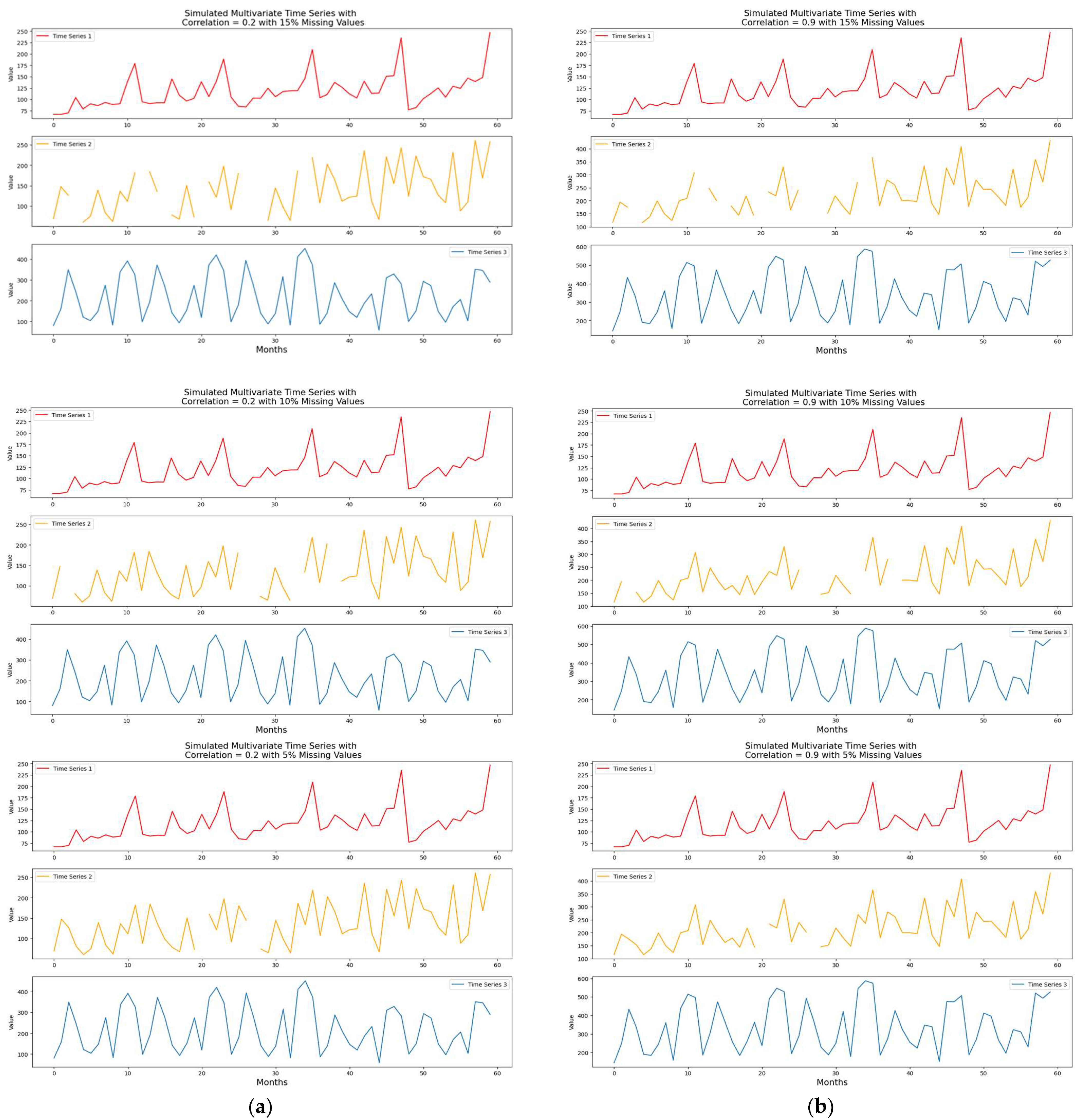
Another study [10] aims to study the relationship between a wider range of correlations, such as 0.1 to 0.99, and bivariate time series forecasting. It concludes that, as correlation increases in simulated data, the overall forecasting accuracy increases. In our study, $\rho = 0.2, 0.9$ are selected to be the designated correlation coefficients computed as in Equations (24) and (25). Two correlated multivariate time series datasets with shifted trends are obtained. Moreover, 15%, 10% and 5% of missing values are considered. Therefore, six simulated time-series datasets are analyzed and modeled in total, and the plots of simulated time series data are presented in Figure 2.

As the correlation increases, the patterns of the time series change; the second and third series obtain more data patterns than the first series. To describe the simulated data, each simulated dataset includes 60 observations (monthly data) with three time series (variables).

4.2. Real Data

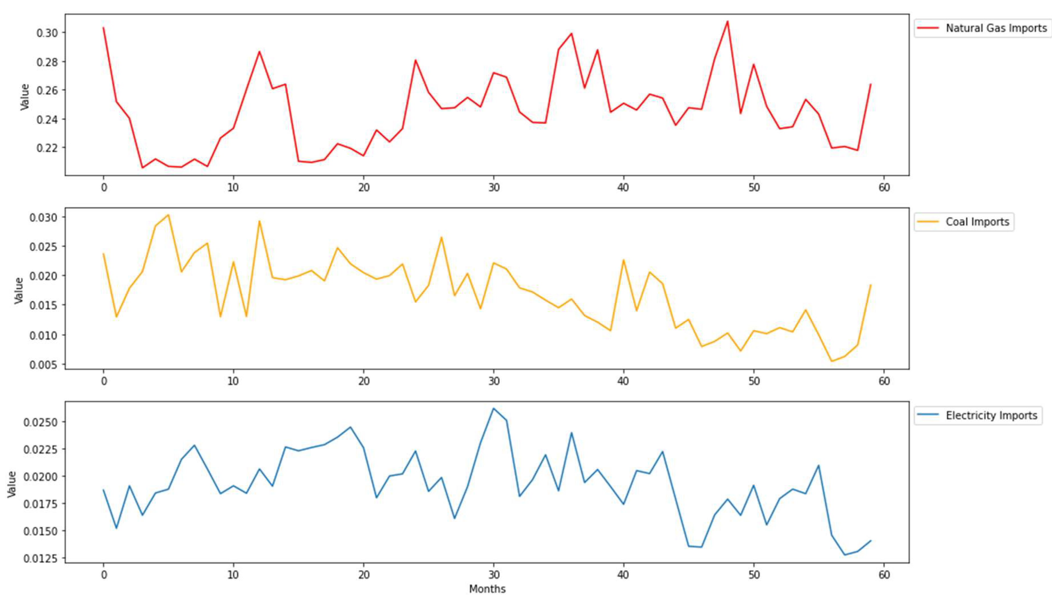
The first real-world dataset used in our study was originally collected from U.S. Energy Information Administration (EIA) Open Data [30]. It comprises monthly energy imports time-series data ranging from January 2014 to December 2018, shown in Figure 3, and it includes three variables: natural gas, coal and electricity imports in Quadrillion British Thermal Units (Btu). The correlation matrix among the three energy imports is given in

Table 5. Correlation matrix of energy import data.

	Natural Gas Imports	Coal Imports	Electricity Imports
Natural Gas Imports	1	−0.19	0.03
Coal Imports	−0.19	1	0.5
Electricity Imports	0.03	0.5	1

, in which correlation coefficients can be investigated. Both coal and electricity imports series show obvious shifted trends, which increase initially and then decrease. Data show more aperiodicity, but no missing data are observed.

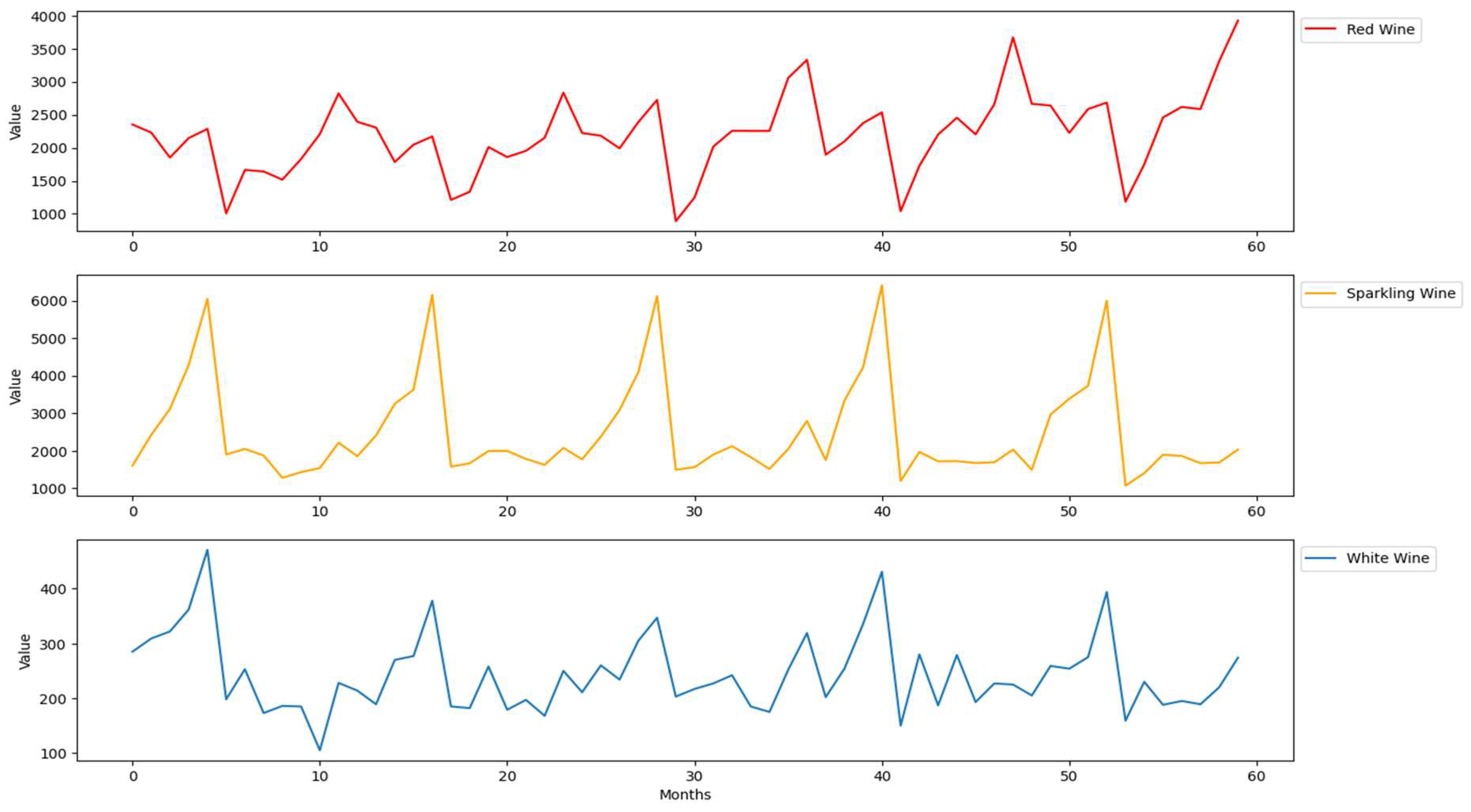
The second real-world dataset was collected from the database of analytical results of the Australian Wine Research Institute’s Commercial Services Group [31]. It comprises monthly wine sales data ranging from August 1990 to July 2005, shown in Figure 4, and it includes three variables: red wine sales, sparking wine sales and white wine sales. Figure 4 shows more regular patterns and no missing values. Red wine sales show increasing trends, sparkling wine sales show regular seasonality patterns, and white wine sales show shifted trends from increased to decreased. The correlation matrix among the three wine sales is given in

Table 6. Correlation matrix of wine sales data.

	Red Wine Sales	Sparkling Wine Sales	White Wine Sales
Red Wine Sales	1	−0.19	0.03
Sparkling Wine Sales	−0.19	1	0.5
White Wine Sales	0.03	0.5	1

. To maintain consistency with the simulated data, these two real datasets include 60 observations with three time series.

4.3. Experimental Design and Framework of Computational Approaches

The experimental design tends to illustrate the modeling strategies for both traditional and AutoML approaches discussed in Section 3 to forecast time series in various lengths, such as 6-month and 12-month forecasts. These strategies specifically address multivariate time-series limitations, including correlation, shifted trends and missing values. All datasets show nonstationarity in the experiments.

To tackle missing values in time series data, imputation methods are necessary, such as pre-AutoML. In our case, missing data are categorized as missing at random (MAR). Under MAR, the complete case analysis is no longer relies on a random sample of the source population, and selection bias is likely to occur [32]. Instead of imputing with the mean of the training set, the proposed method suggests imputing with the mean of the previous and next valid observations. Hence, this approach intends to maximize the seasonality effect and autocorrelation in the training set.

Throughout the whole experiment, all datasets are partitioned temporally: the first 48 months of data points are used for the training set and the last 12 months of data points are used for the test set. The test set aims for prediction, so it is set to unknown. The experimental results represent deterministic outcomes under consistent experiment settings, by fixing random seeds (888). 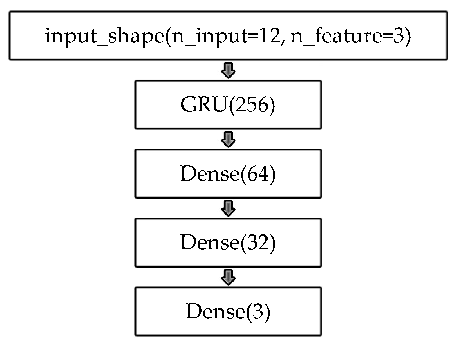After searching the hyperparameters from Table 1 and Table 3, the optimal AutoML-GRU networks are given in Figure 5, as training simulated data with correlation $\rho = 0.9$, shifted trends, and 10% of missing values.

Both traditional and AutoML methods adopt the multi-step ahead forecasting strategy [33]. Each AutoML model trains time series data up to time $t$, and the iterative process of predictions is mathematically expressed in Equations (26)–(28):

$${\widehat{x}}_{t+1}=f\left(x_t,x_{t-1},x_{t-2},\dots ,x_{t-p}\right)$$

(26)

$${\widehat{x}}_{t+2}=f\left({\widehat{x}}_{t+1},x_t,x_{t-1},\dots ,x_{t-p+1}\right)$$

(27)

$$⋮$$

$${\widehat{x}}_{t+h}=f\left({\widehat{x}}_{t+h-1},{\widehat{x}}_{t+h-2},\dots ,{\widehat{x}}_{t+1}\right)$$

(28)

That is, a time series model produces a one-step-ahead prediction, feeds that prediction as input back in the model to predict the next time-step values, and repeats this process to produce multiple future values. This forecasting strategy is efficient for high-frequency time series, such as stock price data.

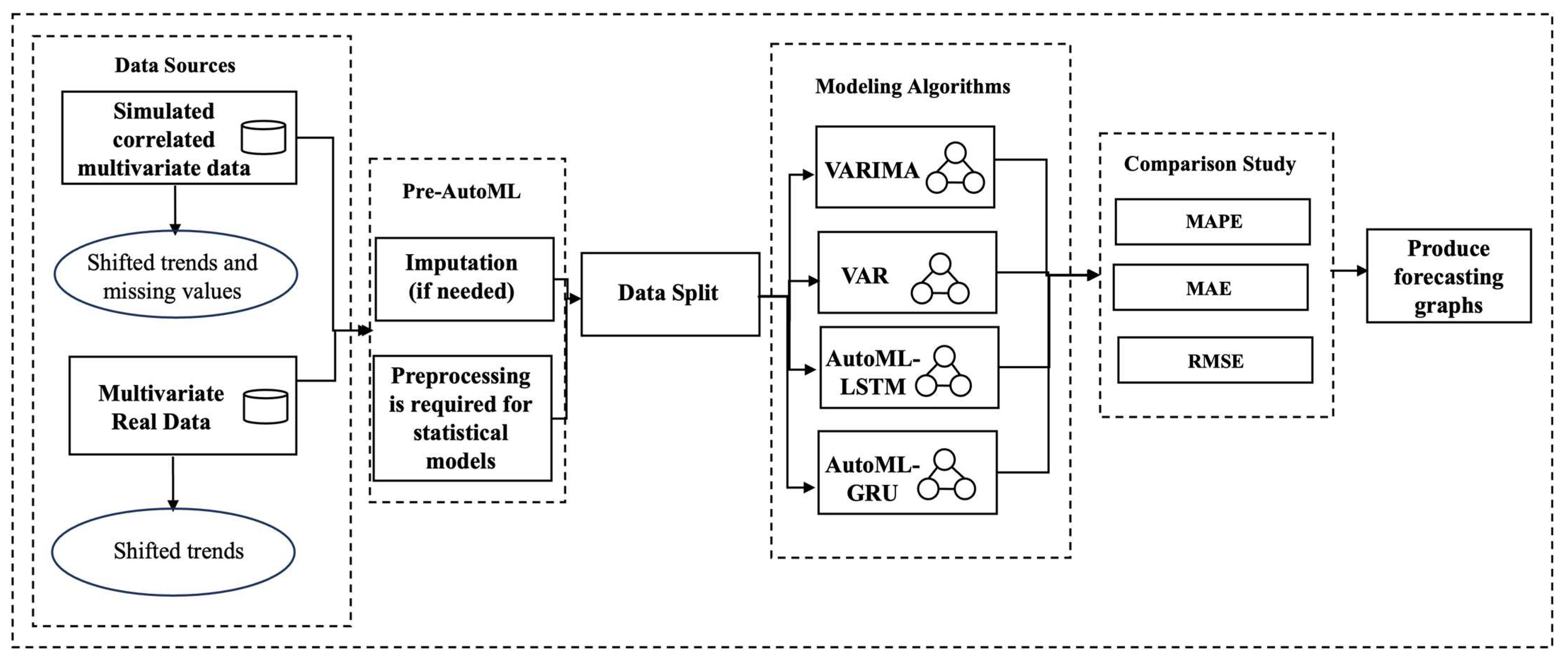
Lastly, Figure 6 summarizes a computational framework of this study, starting from our data source to forecasting graphs.

5. Empirical Findings

This section presents and interprets the empirical results from experiments including forecasting plots and tables of forecasting errors. The discussion is divided into two parts: simulated data and real data. To evaluate the forecasting methods, we aim to investigate the prediction performances with varying lengths such as the first 6 months and 12 months.

Three forecasting accuracy metrics are applied to assess the empirical results: Mean Absolute Percentage Error (MAPE), Mean Absolute Error (MAE) and Root Mean Square Error (RMSE). MAPE and MAE are important measures to evaluation time series forecasts, and RMSE represents a more robust indicator utilized to address zeros and heterogeneous scales. The three metrics are defined in Equations (29)–(31):

$$MAPE=100\%\cdot {\displaystyle \frac{1}{n}}\sum _{t=1}^n\left|{\displaystyle \frac{Y_t-\widehat{Y_t}}{Y_t}} \right|$$

(29)

$$MAE={\displaystyle \frac{1}{n}}\sum _{t=1}^n\left|{\widehat{Y}}_t-Y_t\right|$$

(30)

$$RMSE=\sqrt{{\displaystyle \frac{1}{n}}\sum _{t=1}^n{\left(Y_t-\widehat{Y_t}\right)}^2}$$

(31)

where ${\widehat{Y}}_t$ is the predicted value at time $t$ and $Y_t$ is the observed value at time $t$.

5.1. Modeling Results of Simulated Data

We have evaluated the performance of our proposed method on each simulated dataset and compared it with traditional methods. Each dataset is involved with specific multivariate time series components: correlation $\rho =0.2, 0.9$ and missing values (15%, 10%, 5%). We also demonstrate and investigate the effects taken by those components in simulated data. Therefore,

Table 7. Forecasting results of simulated data ($\rho =0.2$).

Forecasting Length	Models	MAPE (%)	MAE	RMSE	MAPE (%)	MAE	RMSE	MAPE (%)	MAE	RMSE
		Time Series 1			Time Series 2			Time Series 3
							$\rho =0.2$ and 15% of Missing Values
6-Month	AutoML-LSTM	19.5217	18.2212	22.6389	17.9414	27.5165	35.116	20.9145	41.8277	55.2892
	AutoML-GRU	19.0936	17.0478	21.9731	14.5358	22.6779	30.2602	13.821	26.8921	42.3406
	VARIMA-DSDT	122.603	118.0349	131.216	115.5459	167.6963	176.7894	136.7305	211.72	262.35
	VAR-DSDT	103.0095	104.501	120.3628	45.0043	75.6777	95.2355	69.1273	124.3788	164.4332
12-Month	AutoML-LSTM	18.4921	22.6557	27.2228	23.0623	34.1562	40.7921	23.6679	49.3262	64.2154
	AutoML-GRU	14.5594	16.1515	20.0241	15.5994	24.8218	29.5035	17.4936	36.7739	48.8009
	VARIMA-DSDT	108.1622	131.1376	140.2047	112.824	170.6916	177.0365	136.7305	218.4139	254.9315
	VAR-DSDT	102.1687	130.4718	143.6828	55.6185	97.5751	116.286	95.4811	194.2811	225.6852
							$\rho =0.2$ and 10% of Missing Values
6-Month	AutoML-LSTM	19.484	17.5009	20.6844	15.9185	23.7217	28.3145	31.1282	60.7762	79.7135
	AutoML-GRU	23.503	20.5292	23.1644	13.042	22.5135	30.0513	20.6137	38.0427	43.9982
	VARIMA-DSDT	120.0997	115.9994	121.6586	112.9714	164.2101	174.3991	139.2171	214.3317	289.284
	VAR-DSDT	39.7253	44.7831	65.4465	69.8986	112.8137	150.4287	94.3376	202.3646	292.739
12-Month	AutoML-LSTM	14.6271	16.6089	20.1692	17.1879	24.9606	28.031	27.5627	58.718	71.6928
	AutoML-GRU	16.3766	17.9761	24.794	16.8646	30.718	49.8442	15.1601	26.6358	42.1157
	VARIMA-DSDT	106.5648	129.3864	134.5509	112.7262	169.4803	175.4694	133.2859	224.6594	280.0625
	VAR-DSDT	57.5926	81.1735	110.3182	63.7603	100.6041	128.6012	116.8759	265.1223	329.7228
							$\rho =0.2$ and 5% of Missing Values
6-Month	AutoML-LSTM	26.1114	24.2533	28.5834	15.8759	21.4641	27.633	17.914	32.937	44.5564
	AutoML-GRU	11.5857	10.647	13.6801	15.2096	23.5782	28.9968	25.9407	37.1033	44.5402
	VARIMA-DSDT	125.2267	120.5283	128.9939	115.2211	165.5286	177.5111	157.9145	239.1027	303.1924
	VAR-DSDT	115.0755	115.2374	130.054	59.8069	95.4558	133.5278	101.0196	135.9037	169.2814
12-Month	AutoML-LSTM	23.7671	27.283	31.9796	20.0686	26.5207	32.2764	24.9984	53.902	66.4551
	AutoML-GRU	9.6306	11.6155	15.4199	15.3083	25.7021	30.7936	19.6115	30.6145	37.9821
	VARIMA-DSDT	108.3816	130.1262	135.8827	113.4326	169.133	176.371	137.0052	232.257	280.1757
	VAR-DSDT	120.6507	155.5963	176.6874	73.5088	138.7173	181.0712	88.4379	163.4246	213.3957

VAR-DSDT = Deseasonalization and detrend were processed in the data before VAR modeling. VARIMA-DSDT = Deseasonalization and detrend were processed in the data before VARIMA modeling. The lowest forecasting errors are highlighted in bold.

and

Table 8. Forecasting results of simulated data ($\rho =0.9$).

Forecasting Length	Models	MAPE (%)	MAE	RMSE	MAPE (%)	MAE	RMSE	MAPE (%)	MAE	RMSE
		Time Series 1			Time Series 2			Time Series 3
							$\rho =0.9$ and 15% of Missing Values
6-Month	AutoML-LSTM	20.833	20.3299	28.3876	15.8439	33.8396	42.8689	14.7018	43.0448	58.3318
	AutoML-GRU	13.5931	11.8146	14.8193	6.5933	14.6465	17.4962	8.0778	25.5848	34.8507
	VARIMA-DSDT	122.8844	118.1759	129.4884	117.7144	251.1272	261.2753	124.1368	328.1029	385.6576
	VAR-DSDT	103.0095	104.501	120.3628	45.0043	75.6777	95.2355	69.1273	124.3788	164.4322
12-Month	AutoML-LSTM	16.5602	18.9507	25.3561	14.5264	31.3702	41.17	13.513	44.0476	54.7692
	AutoML-GRU	13.6271	17.9349	25.0124	13.0307	40.1109	58.0754	8.3734	31.3857	38.8811
	VARIMA-DSDT	108.1351	130.8931	139.0871	108.5481	261.4883	269.2378	111.1003	349.0975	389.0937
	VAR-DSDT	102.1687	130.4718	143.6828	55.6185	97.5751	116.286	95.4811	194.2811	225.6852
							$\rho =0.9$ and 10% of Missing Values
6-Month	AutoML-LSTM	21.3588	21.3742	27.7026	14.3725	30.1124	33.0758	14.2534	39.7589	49.7027
	AutoML-GRU	18.5757	16.7888	21.2589	13.3921	30.9193	37.0007	14.2241	42.6123	51.6715
	VARIMA-DSDT	119.7852	115.5141	121.0265	114.3552	244.5854	252.3777	122.6272	316.2534	397.9125
	VAR-DSDT	34.2865	35.6824	53.1472	61.0433	143.3702	178.7751	84.0395	269.5379	337.4115
12-Month	AutoML-LSTM	22.1857	27.067	34.7095	15.7351	33.1491	41.606	14.6915	44.6464	53.8752
	AutoML-GRU	11.8929	12.65	17.5917	12.6011	30.3596	36.1632	14.2458	42.9368	52.7601
	VARIMA-DSDT	106.5009	129.315	134.5141	108.168	260.173	266.1182	114.2897	347.9188	404.1513
	VAR-DSDT	64.9119	83.5591	116.8069	91.5281	234.1287	277.4554	79.4724	275.8063	324.9904
							$\rho =0.9$ and 5% of Missing Values
6-Month	AutoML-LSTM	17.2432	15.7322	19.064	14.5084	32.6625	38.6344	12.0459	35.7137	40.3338
	AutoML-GRU	12.0486	11.292	13.9623	12.0396	27.4306	33.0018	12.8693	42.7418	54.2458
	VARIMA-DSDT	124.821	119.7009	128.2114	117.1818	247.595	260.9952	138.8519	355.5474	430.5902
	VAR-DSDT	88.934	94.4706	113.788	83.5176	194.0768	262.2321	102.0491	267.8557	328.2058
12-Month	AutoML-LSTM	16.4004	20.1632	23.94	19.9566	48.5755	56.0581	14.7801	47.5378	53.8842
	AutoML-GRU	9.9674	12.6644	18.1596	14.9878	41.2392	49.835	13.7565	47.0472	53.2534
	VARIMA-DSDT	108.2163	129.4886	134.9586	108.9756	258.3333	267.0621	119.4628	359.3873	413.0938
	VAR-DSDT	79.9745	97.8854	115.8979	103.4277	281.8256	397.2218	104.4277	355.053	444.4077

report the forecasting performance metrics (MAPE, MAE and RMSE) for both 6-month and 12-month datasets. Each partition in the table represents the forecasting errors of simulated data under specific correlations and specific percentages of missing data.

As shown in Table 8, AutoML-GRU outperforms adequately in time series prediction, particularly in correlated data at $\rho =0.9$. The patterns of multivariate data become less complex and easier to capture as the correlation increases to $\rho =0.9$. Meanwhile, overall forecasting errors of correlated data with $\rho =0.9$ are lower than those of correlated data with $\rho =0.2$, which is empirically verified by our article [10].

A detailed analysis of Table 7 and Table 8 reveals that series 1 is a regular seasonal and trended time series, but the overall forecasting errors of series 1 are not as low as those of series 2. Our imputation method obtains reliable and valid predictions in series. 2. Time series 3 comprises shifted trends in the unknown test set, and it is more challenging to predict, so the general forecasting errors are higher than those of the other series. When addressing long-term dependency, the 12-month forecasts modeled by AutoML-GRU achieve more accurately than those produced by AutoML-LSTM. 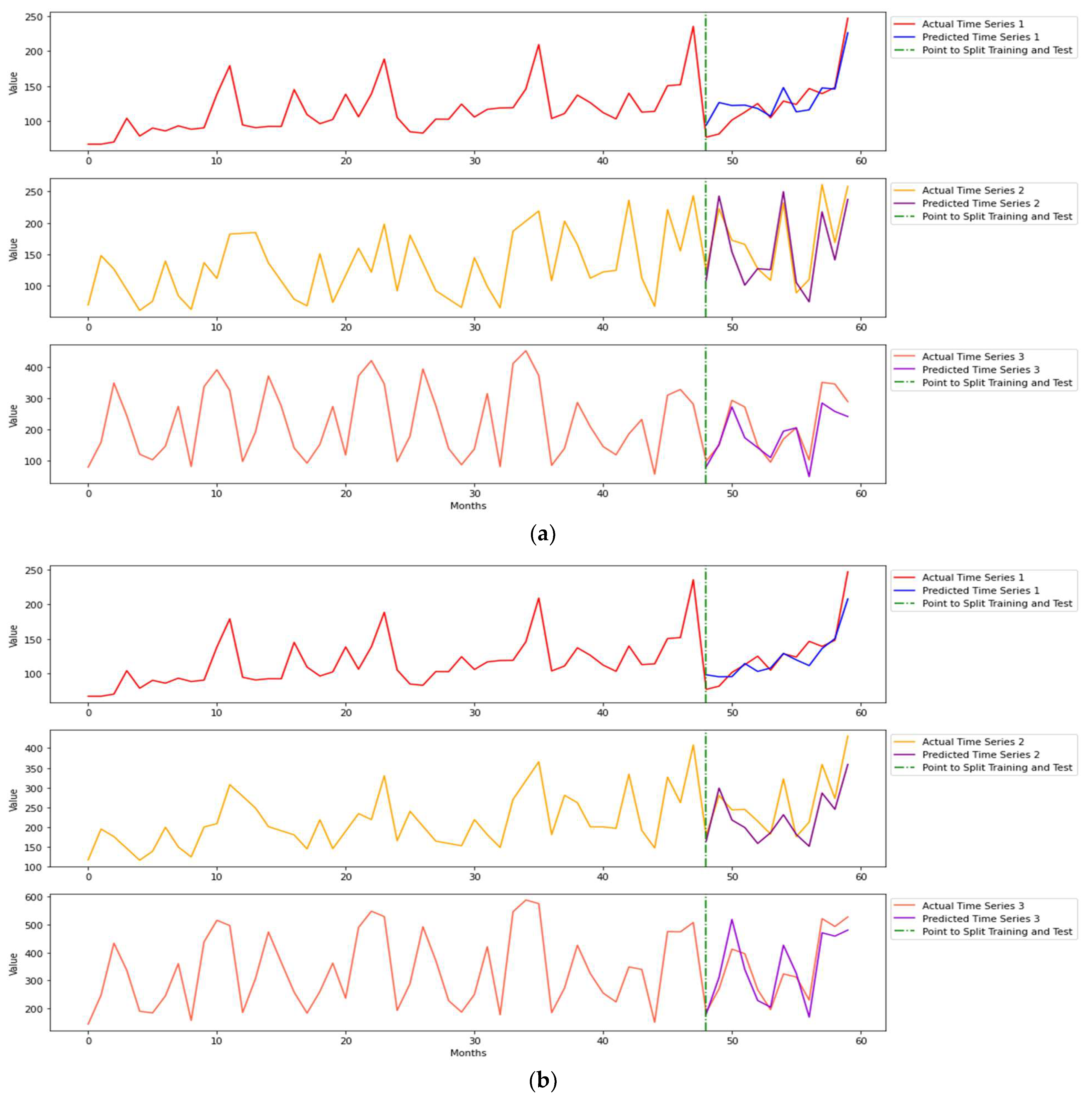Figure 7 shows the forecasting plots modeled by AutoML-GRU. Time series 3 predictions in both datasets are satisfying, because our proposed method is able to learn the shiftiness of dependency. The 12-month forecasting MAPE of the time series 3 of $\rho =0.9$ data is decreased by 52.13% from that of time series 3 for $\rho =0.2$ data.

AutoML-LSTM is a competitive alternative for modeling, resulting in some low forecasting errors. For time series 3 for simulated data with $\rho = 0.2$ and 5% missing data, the six-month MAPE of AutoML-LSTM is 30.94% lower than that of AutoML-GRU. For time series 1 for simulated data with $\rho = 0.2$ and 10% missing data, the 12-month MAPE of AutoML-LSTM is 10.68% lower than that of GRU. Combining forecasting results and plots, AutML-GRU forecasts involve some fluctuations but generally result in higher forecasting accuracy and efficiency. Empirically speaking, our proposed method tends to exhibit relatively superior performance in simulated correlated data as the correlation increases. The forecasting performances of traditional methods yield noticeably larger errors in the experiments. The simulated data initially assume linearity, but a linear model is not the optimal choice when correlation, missing values and shifted trends are accounted for.

5.2. Modeling Results of Real Data

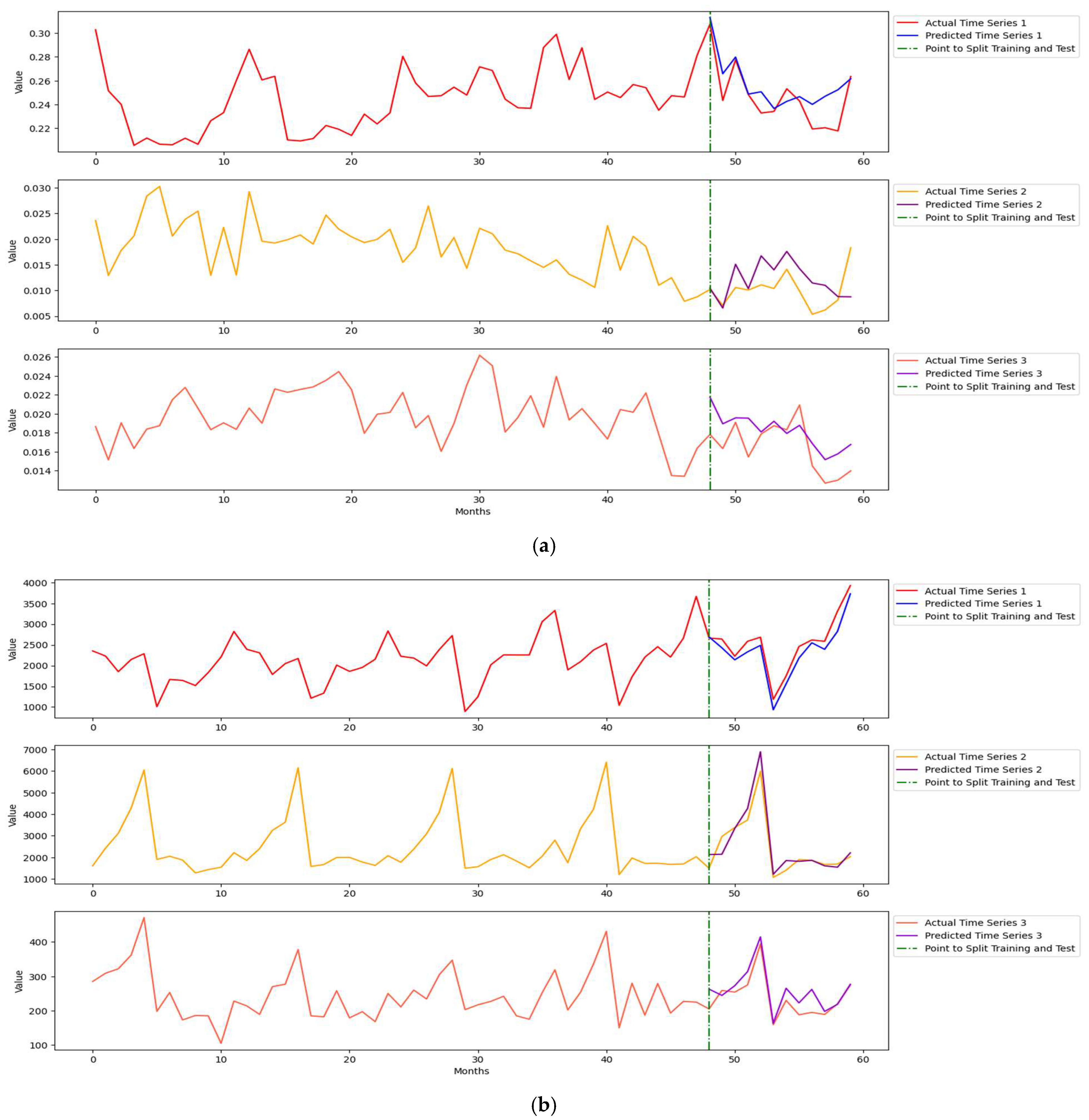
The evaluation strategy for modeling real data is the same as that for modeling simulated data. Although correlation, shifted trends and seasonality are also temporal characteristics presented in both real datasets, Figure 8 demonstrates more complex multivariate temporal patterns with higher noise and aperiodicity, whereas Figure 4 shows clearer seasonality with slightly shifted trends. Both Figure 8a and

Table 9. Forecasting results of real data.

Forecasting Length	Models	MAPE (%)	MAE	RMSE	MAPE (%)	MAE	RMSE	MAPE (%)	MAE	RMSE
		Time Series 1			Time Series 2			Time Series 3
		Energy Imports Data
		Natural Gas Imports			Coal Imports			Electricity Imports
6-Month	AutoML-LSTM	6.2805	0.0153	0.0192	39.078	0.0039	0.0046	11.8613	0.002	0.0027
	AutoML-GRU	3.4636	0.0085	0.012	23.5765	0.0025	0.0033	11.7929	0.002	0.0026
	VARIMA-DSDT	101.7672	0.262	0.2648	112.348	0.0107	0.014	99.6808	0.0174	0.0175
	VAR-DSDT	12.9235	0.0318	0.0423	33.114	0.0029	0.0039	21.4422	0.0036	0.0044
12-Month	AutoML-LSTM	6.4845	0.0152	0.0185	36.1085	0.0037	0.0046	8.1469	0.0014	0.0018
	AutoML-GRU	5.3732	0.0124	0.0166	38.4325	0.0037	0.0046	13.3467	0.0021	0.0024
	VARIMA-DSDT	99.3144	0.2452	0.2478	110.3698	0.0109	0.0133	99.6369	0.0166	0.017
	VAR-DSDT	15.4663	0.0367	0.0492	81.8833	0.0068	0.0092	26.0903	0.0041	0.0047
		Wine Sales Data
		Red Wine Sales			Sparkling Wine Sales			White Wine Sales
6-Month	AutoML-LSTM	10.9233	225.6889	320.052	23.9588	604.6586	695.7098	9.7509	26.2472	32.8939
	AutoML-GRU	8.5649	171.5033	191.5774	19.095	514.1963	604.9944	10.5546	25.84	31.2254
	VARIMA-DSDT	120.3868	2671.4285	2726.771	130.0732	3020.9421	3465.1125	109.5165	268.8747	282.6836
	VAR-DSDT	31.7732	693.3978	827.7707	98.8852	1670.0156	2354.0755	36.497	88.5362	108.3871
12-Month	AutoML-LSTM	10.464	243.5829	321.8183	15.1477	353.6386	500.7908	12.0495	28.2364	33.7988
	AutoML-GRU	8.6075	203.1717	232.6027	14.3415	333.5842	452.9031	11.4872	25.4314	32.7445
	VARIMA-DSDT	104.2866	2555.1498	2620.7809	116.9664	2413.4892	2811.3906	102.0765	234.0531	245.2921
	VAR-DSDT	45.2214	1142.1581	1303.0388	68.115	1163.7218	1736.0898	35.8367	84.4286	102.417

clearly show that AutoML-GRU outperforms in forecasting both 6-month and 12-month natural gas imports, because of the evident increasing trends and seasonality. The 6-month MAPE in forecasting natural gas imports modeled by AutoML-GRU is 44.85% lower than that by Auto-LSTM. In the case of coal and electricity import data, the trend begins to decline gradually from the 12th month of the training period, though with noticeable fluctuations. Figure 8a presents the forecasting plots, demonstrating that AutoML methods can capture decreasing trends. However, the 6-month and 12-month forecasting performances by AutoML-LSTM in predicting electricity imports outperform other models, because of the complexity of LSTM networks. Figure 8b and Table 9 present the wine sales forecasting performance. AutoML-GRU forecasts outperform in predicting all-length and three series, except in the 6-month MAPE of white wine sales, with a value 7.61% lower than that of AutoML-LSTM. Both [10] and this research have indicated that traditional methods neither learn the correlations among bivariate time series nor produce subpar forecasting performances.

6. Discussion and Conclusions

One significant advantage of most traditional time series methods is the assumption of linearity. Thus, ARIMA, VARIMA and VAR have less computational effort and high interpretability, but they experience more preprocessing efforts and lower prediction accuracy. At present, time series are more complex, aperiodic and high-dimensional, requiring a powerful alternative. Within the AutoML search space, both LSTM and GRU networks are recommended due to their forecasting performance, with each addressing certain limitations of multivariate time series. After missing data imputation, GRU with the simpler NN architecture outperforms because trends and seasonality can be identified and learnable. On the other hand, the LSTM network is a powerful alternative if the task focuses on solving long-term dependency. Compared with traditional forecasting methods, LSTM and GRU are DL models, which introduce expensive computations. That is, they can reach some hidden information of time series and allow them to be learned. These two NN constructions within the AutoML framework can be further optimized by considering more factors in the experiments. This article introduces initial GRU applications to multivariate time series analysis; however, similar to other NN architectures, GRUs operate largely as “black boxes” with limited interpretability. In addition, several implementation details and practical considerations remain open issues that will be addressed in future research. A multi-step recursive forecasting strategy is used to predict time series due to its effectiveness in capturing specific patterns for coherent prediction and its compatibility in correlated time series. However, the multi-step direct method is well-suited for long-term predictions and volatile time series. In future research, a comparative analysis can be conducted to evaluate direct, hybrid and recursive forecasting strategies, rather than limiting the comparison with statistical methods.

In this article, we proposed AutoML approaches to forecasting correlated multivariate time series consisting of shifted trends and missing data, by utilizing GRUs. AutoML aims to solve a time series task in an automated way so that little manual effort is required [34]. When processing nonstationary multivariate data, our proposed method does not require preprocessing. The empirical evidence from simulated and real data indicates that LSTM and GRU networks significantly outperform traditional methods in the terms of manual intervention, preprocessing and prediction accuracy. Even though the computational costs of conventional forecasting methods are low, AutoML and NN systems can learn to address long-term dependencies across multiple variables in data. The advantages of LSTM and GRU stand out because they are able to tackle some multivariate time series problems but find it challenging to address all problems simultaneously. As AutoML aims to identify the suitable and best-fit models, our research exhibits and empirically shows that GRU is highly recommended for multivariate time series tasks characterized by clearer seasonality and shifted trend patterns. In contrast, LSTM serves as a quality alternative for tasks involving more complex structures, such as aperiodicity and noise. The nature of AutoML may allow us to overlook the lack of interpretability, as it is primarily designed to assist non-experts without prior technical expertise. The proposed AutoML frameworks are user-friendly and efficient, particularly for time series forecasting tasks, while effectively capturing essential domain-specific features.

Hence, our research goals and hypotheses have been achieved along with empirical evidence. The utilization of AutoML approaches have been discussed and demonstrated comprehensively, addressing specific multivariate time series characteristics or limitations. Compared to traditional methods, the forecasting performances of proposed methods achieve enhanced accuracy.

7. Future Work

To build on this article, an AutoML approach can be proposed to solve the task of multivariate time series with covariates. Usually, multivariate time-series data come with additional variables, such as socio-economic status and marital status.

A further study would incorporate more time series challenges, such as extreme and abrupt events in time series. For instance, COVID-19 had a significant impact on the world, from our daily lives to the global economy. Considering extreme events as factors in the time series data, AutoML solutions can be developed based on their effects. From the perspective of traditional methods, VARFIMA can be considered due to its ability to capture long-term memory and cross-correlations between series.