Data Preprocessing and Feature Engineering for Data Mining: Techniques, Tools, and Best Practices

Abstract

Data preprocessing and feature engineering play key roles in data mining initiatives, as they have a significant impact on the accuracy, reproducibility, and interpretability of analytical results. This review presents an analysis of state-of-the-art techniques and tools that can be used in data input preparation and data manipulation to be processed by mining tasks in diverse application scenarios. Additionally, basic preprocessing techniques are discussed, including data cleaning, normalisation, and encoding, as well as more sophisticated approaches regarding feature construction, selection, and dimensionality reduction. This work considers manual and automated methods, highlighting their integration in reproducible, large-scale pipelines by leveraging modern libraries. We also discuss assessment methods of preprocessing effects on precision, stability, and bias–variance trade-offs for models, as well as pipeline integrity monitoring, when operating environments vary. We focus on emerging issues regarding scalability, fairness, and interpretability, as well as future directions involving adaptive preprocessing and automation guided by ethically sound design philosophies. This work aims to benefit both professionals and researchers by shedding light on best practices, while acknowledging existing research questions and innovation opportunities.

1. Introduction

Preprocessing and feature engineering are essential data mining (DM) building blocks that enable the conversion of varying and crude inputs into interpretable and standardised forms. The data involved in real-life applications often pose challenges such as noise, sparsity, inconsistency, imbalance, and variability of distribution. Furthermore, datasets are often limited by practical scale-related limitations, with additional issues related to data management and challenges regarding data replication, all crucial to ensure repeatability and verifiable outcomes. It is necessary to treat preprocessing as an essential component of an end-to-end data pipeline requiring systematic methods that include cleansing and transformation of data with standardised encoding and normalisation to feature generation and selection, along with dimensionality reduction (DR). These are necessary to align with essential analytical requirements related to accuracy, efficiency, robustness, and fairness.

This paper aims to guide practitioners in building pipelines to withstand data leakage, ensure verifiability, and maintain reliability with changes to data, models, and requirements by integrating methodological knowledge with comprehensive details on selected tools and practical design frameworks.

1.1. Role of Preprocessing in DM

Data preprocessing is a step in DM [1]. It can be viewed as a critical go-between process that bridges unpolished, often disorganised or noisy datasets and sophisticated algorithms that distil knowledge or create predictive models. Without preprocessing, even very advanced models can perform poorly, due to incompleteness, outliers, missing values, or non-pertinent attributes [2,3]. Practically, preprocessing enhances input data quality and, thus, the accuracy of results. In addition, it ensures that models run on datasets with completeness, a systematic structure, and absence of distortion, which, otherwise, can contaminate results or reduce interpretability.

Preprocessing involves a set of operations, including data cleaning, transformation, normalisation, feature encoding, and DR [1,4]. These procedures affect the effectiveness of DM methods, especially in scenarios where procedures rely on differences in input distributions, feature scale discrepancies, or the level of the discrepancies of sparsity. For instance, unnormalised numerical features have the potential to add bias to distance-based clustering procedures, while encoded categorical features have the capacity to inhibit strong model development.

Additionally, preprocessing contributes to model fairness and effectiveness by reducing noise, as well as by dealing with the intrinsic structural data imbalances. For example, in [5], the authors discuss how various ML pipeline stages can introduce or mitigate bias, while preprocessing facilitates automation within the data pipelines, further contributing to increased reproducibility, scalability, and transferability in application scenarios. As the dependency of core sectors, including finance, healthcare, and governance, has increased, effective preprocessing has been transformed from a subject of technical interest to an essential methodological framework.

1.2. Motivating Examples and Performance Impact

For a binary classification task like forecasting credit defaults, failure to compensate for missing income data, for example, can lead to misclassification of high-risk individuals. Deploying strong imputation methods—like k-nearest neighbours or regression-based imputation—can have a significant impact on both precision and recall. Equally, when analysing medical diagnoses based on patient histories, variations in symptom coding or measurement scales can have negative effects on the efficiency of machine learning (ML) techniques. Standardisation and normalisation procedures performed on data from different sources not only produce gains in mean precision but also increase interpretability [6,7].

In healthcare, leakage-safe imputation and encoding must preserve rare but clinically salient events; robust scaling is preferable to minimise the effect of extreme laboratory values, and subgroup analyses should accompany any missing-data strategy to avoid disparate impact [2]. In finance, time-aware validation (blocked or forward-chaining) is mandatory; encoders with target information must be fitted out-of-fold, and drift monitoring should track segment-level shifts (e.g., by product or region) to trigger recalibration [1].

Even basic preprocessing can have significant impact. For example, feature scaling represents an essential prerequisite to optimisation-based approaches like support vector machines and logistic regression [6,8]. Insufficient scaling can hinder or downright prevent convergence, leading to a model becoming stuck in suboptimal solutions. For time-series mining, feature misalignment can prevent critical patterns from being identified. Another area of preprocessing, feature engineering, provides larger boosts to performance in place of changes made to a model’s hyperparameters. In many cases, top-performing solutions rely upon carefully crafted feature transformations, instead of overly complex models [9].

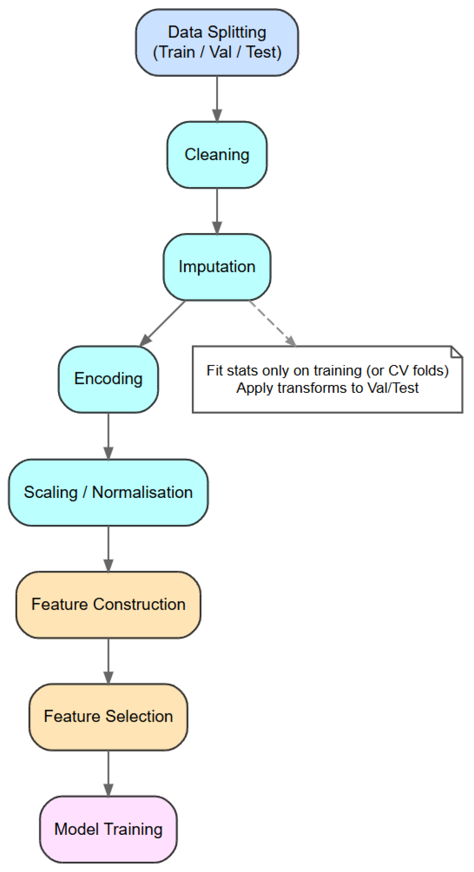
Additionally, automated preprocessing packages (implemented via scikit-learn–style pipelines or low-code frameworks such as PyCaret) show that simple models exposed to uniform preprocessing can outperform state-of-the-art models trained from unprocessed data [8,10]. Automated ML (AutoML) benchmarks report top-tier performance for pipeline-driven tools across binary, multiclass, and multilabel tasks [11,12]. Ref. [13] also ascertains through domain-specific experiments that preprocessing choices can outweigh hyperparameter tuning in their effect on downstream accuracy, raising preprocessing as both a scientific and an engineering priority in DM. An overview of the end-to-end preprocessing pipeline referenced throughout this review is shown in Figure 1, followed by

Table 1. Cross-domain preprocessing requirements and safeguards.

Domain	Typical Risks	Required Safeguards
Healthcare	Rare-event dilution; heterogeneous coding; extreme lab values; subgroup harm	Leakage-safe imputation/encoding; robust scaling; subgroup analyses; transparent logging
Finance	Temporal leakage; concept drift; high-cardinality categoricals; regime shifts	Blocked/forward-chaining cross-validation (CV); out-of-fold encoders; drift monitoring; scheduled recalibration
Industrial IoT/Time-series	Non-stationarity; bursty missingness; sensor bias; misalignment	Windowed/context-aware imputation; detrending/denoising; per-sensor scaling; segment-wise validation
E-commerce (tabular)	High cardinality; seasonality; sparse interactions	Hashing; frequency/target encoders; time-aware CV; interaction features; leakage checks in promotions

, which summarises typical risks and the required safeguards across domains.

Recent evaluations underline that evaluation protocol and leakage control determine the credibility of reported gains; widespread, often subtle leakage has been documented across domains [14]. For temporally ordered data, blocked or forward-chaining validation is recommended to avoid look-ahead bias and information bleed [15].

1.3. Objectives of This Review

This review has four objectives, corresponding with the need for transparency, critical integration, and practically useful guidance identified in the literature:

1.

Develop a unifying framework: Develop a context-specific taxonomy that integrates preprocessing and feature engineering as systematic phases (cleaning, transformation, construction, selection, reduction), while incorporating decision variables such as dataset dimensions, interpretability, and computational resources.

2.

Evaluate techniques critically: Make comparative assessments of imputation, encoding, feature selection, and DR techniques, including linked risks, trade-offs, and recorded failure instances.

3.

Describe practical heuristics: Specify requirements as numerical values (e.g., sample sizes of autoencoders and variance filter thresholds) and shed light on common pipeline design choices (e.g., fitting training-only scalers) to enhance reproducibility and tackle data leakage.

4.

Codify best practices: Establish definitive design patterns and procedural guidelines for direct implementation by practitioners, covering topics such as leakage management, CV, fairness auditing, and monitoring in realistic deployment scenarios.

These objectives distinguish this work from preceding surveys, as it moves from a description to a systematic, critical, and prescriptive contribution.

1.4. Scope and Structure of the Review

This research provides a thorough analysis of data preprocessing and feature engineering methodologies, focusing mainly on structured data. The aim is to incorporate basic and advanced automated or manual techniques, as well as assessing their impact on tasks, such as classification, clustering, and regression. Consideration has been given to optimise techniques allowing for reproducibility, interpretability, and streamlined workflow, qualities becoming ever more critical in real use cases and regulatory compliance [16].

First, we discuss data cleaning and transformation concepts, such as handling missing values and outliers, as well as scaling and encoding. Then, we delve into an in-depth analysis of feature engineering and selection methods, including filter, wrapper, and embedded methods. We further discuss DR, handling standard linear and nonlinear embedding methods. We also discuss different automation libraries and tools, which allow for preprocessing pipelines to be created easily. In subsequent sections, we discuss selection procedures and how they impact model assessment, and we explain how best practices help to increase system robustness, scalability, and maintainability regardless of size and complexity. Finally, we summarise by highlighting challenges and future research directions, mainly automation, interpretability, and scalability.

1.5. Novelty and Contribution

This work advances the state of the art by going beyond descriptive surveys and making three original contributions:

1.

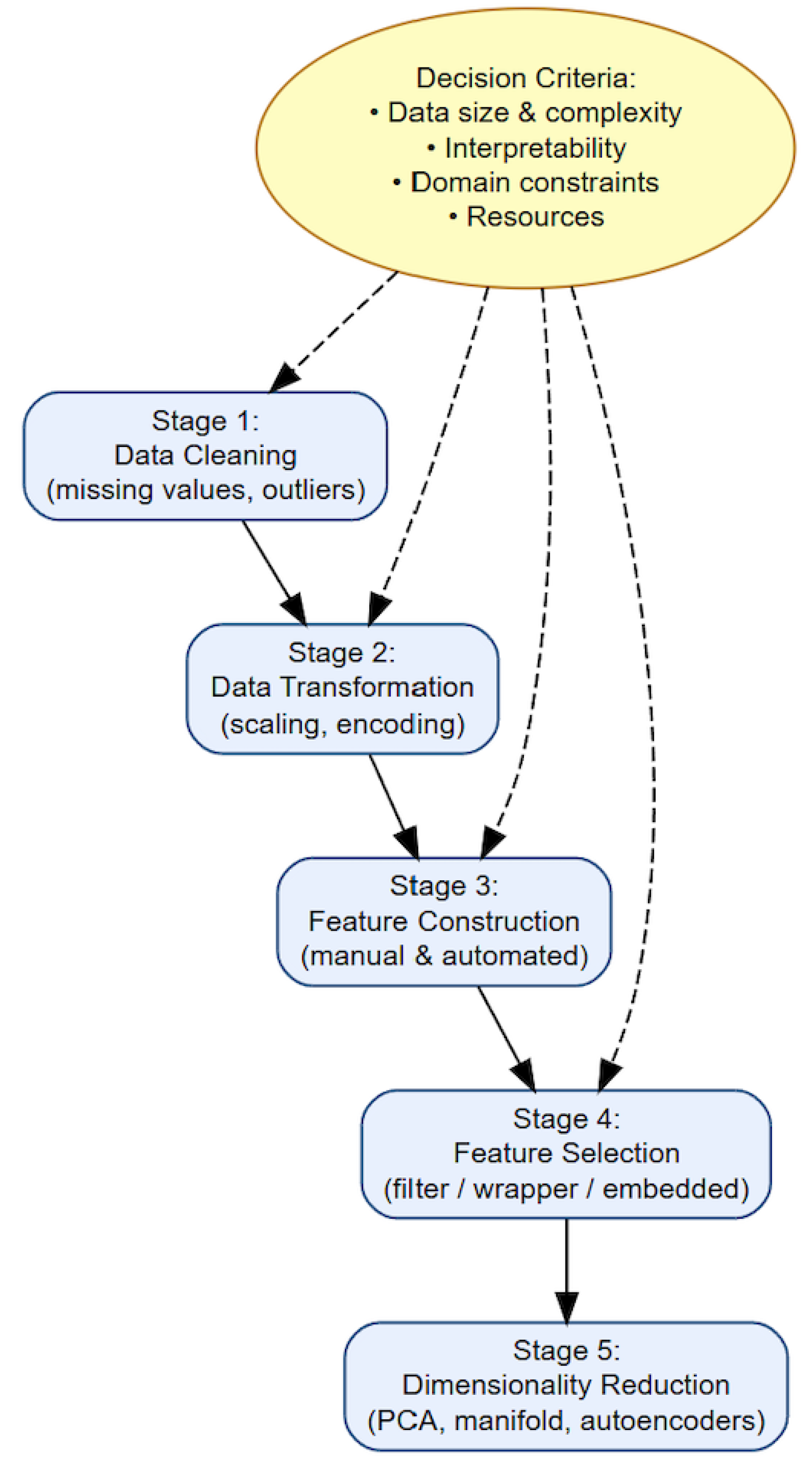
We propose a unifying framework (Section 2), which systematically organises data preprocessing and feature engineering into five pipeline stages (cleaning, transformation, construction, selection, reduction), while explicitly linking them to decision criteria (dataset size, interpretability, domain constraints, computational resources).

2.

We provide comparative tables and method-level evaluations that highlight trade-offs, risks, and common failure cases across imputation, encoding, selection, and DR.

3.

We highlight best engineering practices, including serialisation, experiment tracking, and monitoring for drift and health, such that methodologies are always reliably transferable from the realm of notebooks into production environments.

These contributions position this review not just as a consolidation of methods existing in the literature but as an integrative framework and prescriptive guide for researchers.

2. Conceptual Framework: A Context-Aware Taxonomy of Data Preprocessing and Feature Engineering

This section presents a unifying conceptual framework. It organises data preprocessing and feature engineering into a context-aware taxonomy, which emphasises two dimensions. The stage of the preprocessing pipeline, ranging from cleaning to DR on the one hand, and the approach modality, distinguishing manual, expert-driven procedures from automated, algorithm-driven solutions on the other. It also incorporates decision criteria, such as dataset size, interpretability requirements, domain constraints, and computational resources.

The first stage of the taxonomy is data cleaning, which encompasses the detection and correction of missing values and outliers. Manual strategies, such as rule-based deletion or domain-specific imputations remain common in practice [17]. Automated techniques, however, have grown in prominence: k-nearest neighbours imputation exploits local similarity structures [18], and regression imputation leverages inter-feature relationships [7]. Expectation–maximisation and multiple imputation provide statistically principled treatment under the Missing At Random assumption [18], and deep learning models, including autoencoder-based imputers, capture nonlinear dependencies but require substantial training data and careful tuning [18,19,20].

Outlier handling follows a similar duality: domain experts may flag suspicious points manually, while algorithmic approaches include statistical thresholds, clustering-based detectors, and scalable methods, such as Isolation Forest [21]. Crucially, as Refs. [22,23,24] emphasise, decisions about whether to retain or remove outliers must be informed by the domain context, since extreme values may represent valid and meaningful cases (e.g., fraud or rare diseases).

The second stage includes data transformation, so variables are readied for algorithmic application through scaling and encoding. Based on exploratory data analysis of non-scalar distributions, one might introduce manual (e.g., logarithmic or square-root) transformations, while automated scaling methods introduce z-score standardisation or min-max scaling across the entire feature space. These stages are key to attaining stability in algorithmic performance depending on distances and gradients [25,26].

Categorical variables introduce an anomaly: one-hot encoding maintains the integrity of nominal characteristics while inducing an increase in the number of dimensions [27]. Ordinal encoding is justified only if the categories represent some kind of order. Automated encoders, as target and frequency encoding or entity embeddings, are capable of identifying predictive signals or relational patterns but induce leakage and bias or reduce interpretability [27]. The selection of encoding techniques directly intertwines with the modelling scenario and the need for interpretability corresponding to the application scenario.

The third stage is feature construction, in which raw attributes are supplemented or transfigured into variables with greater information content. Manual feature engineering, based on domain understanding, is still potent: scientists can construct domain-specific scores, ratios, or indices that embody theoretical constructs [28]. Automated construction is increasingly tractable using tools like deep feature synthesis [28] and AutoML systems [9,29], which algorithmically generate large sets of candidate features. The literature demonstrates that hybrid systems, blending automated generation with expert knowledge, frequently yield the most robust outcomes, as they have the advantages of machine-driven discovery, as well as human interpretability.

The fourth stage is feature selection, where a subset of variables is left for modelling. Filter techniques rank features according to statistical criteria and are fast but might miss interactions [30]. Wrapper techniques search iteratively over subsets with a learning algorithm and usually achieve higher precision at the expense of exponential computation [30]. Embedded techniques build selection into model training, for instance using regularisation penalties or a tree-based measure of variable importance, and find a balance between performance and speed [31]. Each class comes with trade-offs, and the selection relies not only on available computational power but also on what kind of stability and interpretability is required.

The last stage, DR, is used to compress feature space, thus counteracting the curse of dimensionality and improving computational speed. Principal component analysis (PCA) is established as the default linear method [30], while nonlinear manifold learning methods, such as t-Distributed Stochastic Neighbour Embedding (t-SNE) and Uniform Manifold Approximation and Projection (UMAP), and deep autoencoders [32,33] are capable of preserving more complex structures. However, as suggested in the literature, the interpretability of the applied transformations may vary significantly: components resulting from PCA may sometimes correspond to interpretable constructs, while those from neural embeddings usually remain opaque. Because of that, the decision to apply DR needs a careful consideration of the benefits of preserving variance and computational speed against potential loss of semantic interpretability.

Across all five stages, the taxonomy incorporates decision criteria that determine whether manual or automated methods are preferable. Small or sparse datasets often favour simple or manual techniques to avoid overfitting [7,15], while large, high-dimensional datasets typically require automated solutions for scalability [11]. Applications in healthcare, finance, or other regulated domains prioritise interpretability and fairness, which biases choices toward transparent preprocessing [27,34]. Domain constraints, such as regulatory rules or known causal structures, may mandate or forbid certain transformations [23,34]. Finally, computational budgets influence feasibility: wrappers and deep autoencoders deliver strong performance but are resource-intensive [31,33].

The proposed framework is defined in Figure 2 and combines the five stages of the preprocessing as a single complete pipeline and connects each of them with the final decision criteria.

3. Data Cleaning and Transformation

This section addresses Stages 1 and 2 illustrated in Figure 2, which represent the passage from raw, noisy inputs to representations amenable to modelling. Stage 1, or cleaning, restores data validity in the management of missing values and outlier detection and correction, while Stage 2, or transformation, brings feature spaces into alignment using normalisation or scaling and categorical coding. Together, these steps reduce bias, stabilise learning algorithms, and preserve a strong signal for downstream modelling.

3.1. Handling Missing Values

Missing values are frequent in real-world datasets, coming from various sources, such as sensor failures, human entry errors, integration mismatches, or intentional omission [1]. Missing data can significantly bias model outputs and prevent the application of some algorithms that require complete input vectors [7]. For this reason, missing value handling is often the first necessary step in a preprocessing pipeline.

The easiest initial approach is deletion—either columnwise (removing attributes) or listwise (removing rows)—but it is appropriate only if missing data is minimal and randomly dispersed. Unbiasedness holds only under Missing Completely At Random (MCAR). In realistic Missing At Random (MAR)/ Missing Not At Random (MNAR) settings, deletion reduces power and introduces selection bias [7]. In more realistic scenarios, especially where missingness is systematic or extensive, deletion will lead to loss of information and sample bias. As a substitute, imputation techniques are employed to input missing values in a statistically or contextually informed manner. Simple imputation techniques, such as mean, median, or mode imputation, are favoured due to simplicity but assume feature symmetry and may distort relationships or distributions. Replacing with a single summary value shrinks variance and attenuates correlations, inflating apparent model stability [7].

Beyond deletion, imputation strategies span summary-based (mean/median/mode), instance-based (k-NN) [17,35], regression-based, and model-based approaches (EM, multiple imputation) [36], as well as recent deep-learning variants (autoencoder-based) [37]. Deep models tend to work best in large-sample regimes with careful regularisation, whereas in small-n or sparse settings they may underperform simpler alternatives. Method performance also hinges on the distance metric and feature scaling (local neighbourhoods become noisy in high dimensions) [35]. Deterministic regression fills underestimate uncertainty and can overfit training structure—hence the preference for multiple imputation when feasible [7]. Even for principled estimators, convergence and model misspecification can propagate bias [36]. The choice of imputation method should be guided not only by the proportion of missingness but also by its mechanism (MCAR/MAR/MNAR) and the assumptions of the downstream modelling task, especially in clinical contexts [17].

Evaluation can be performed via synthetic experiments, CV, and downstream model comparisons. To avoid redundancy, we centralise method-level specifics in

Table 2. Overview of common missing-value handling techniques with advantages, limitations, and indicative data regimes.

Technique	Advantages	Limitations	Data Regime (Rule-of-Thumb)
Listwise Deletion	Simple; no computation	Unbiased only under MCAR; information loss; selection bias if MAR/MNAR [7]	Overall missingness ≲ 5–10% and MCAR plausibly satisfied; otherwise avoid.
Columnwise Deletion	Removes attributes with pervasive missingness	Discards potentially informative variables; reduces model capacity [7]	Drop a feature when missingness ≳ 40–60% and low predictive value in screening.
Mean/Median/ Mode Imputation	Fast; easy to implement	Shrinks variance; attenuates correlations; distorts distributions [7]	Small-n, low missingness (≲10–20%) with roughly unimodal/ symmetric features.
k-NN Imputation	Captures local structure; non-parametric	Sensitive to distance metric and scaling; degrades in high dimension/ sparsity [35]	$n\gtrsim {10}^3$ (often ${10}^3–{10}^4$) with scaled features; moderate dimensionality; $k\in [3,10]$.
Regression Imputation	Preserves multivariate relations	Underestimates uncertainty; overfitting risk if deterministic [7]	Moderate n with stable relations; prefer multiple imputation when feasible.
Expectation–Maximisation (EM)/ Multiple Imputation	Statistically principled; models uncertainty under MAR	Model/init sensitivity; more complex to tune [36]	$n\gtrsim 5\times {10}^2$ (often $5\times {10}^2–{10}^3$); MAR plausible; $m\ge 5–10$ imputations.
Autoencoder-based Imputation	Handles nonlinear dependencies; learns latent structure [37]	Data- and tuning-hungry; small-n can underperform simple baselines	Large-sample regimes: typically $n\gtrsim {10}^4$ total (or ≳${10}^3$ per class) with sufficient capacity; otherwise prefer simpler methods.

“Data regime” values are indicative practitioner ranges (rule-of-thumb). Actual thresholds are dataset- and mechanism-dependent and should be tuned via sensitivity analysis. Evidence synthesised from the literature in this work.

and keep the narrative focused on decision drivers (missingness mechanism, data regime, and target task). Table 2 provides a comparative overview of common missing-value handling methods, highlighting their key assumptions, advantages, and limitations to guide appropriate selection in real-world scenarios.

Comparative studies confirm that no single imputer dominates across mechanisms or regimes and that deep architectures typically require larger samples or strong inductive structure to be competitive [18,19,20]. These ranges operationalise that guidance. Precise cut-offs remain dataset-dependent.

3.2. Outlier Detection and Correction

Outliers are observations that differ substantially from the majority of observations and may result from errors in data entry, variability due to measurement, or rare but real events [24,38]. Outliers can cause bias in statistical averages and significantly reduce the effectiveness of algorithms that are sensitive to them, particularly those based on distance measures or parametric modelling approaches. For instance, the presence of a single outlier can skew the computation of the mean, inflate the variance, and mislead algorithms, such as k-means clustering or linear regression.

The identification of outliers involves both univariate and multivariate approaches. For a univariate analysis, outliers can be identified by z-scores by using interquartile ranges (IQRs), boxplots, or similar methods. For a multivariate case, however, identification of outliers becomes more complex and can be achieved by using Mahalanobis distance; clustering-based methods, such as Density-Based Spatial Clustering of Applications with Noise (DBSCAN); or density-based models, such as Local Outlier Factor (LOF), which flag points whose local reachability density is much lower than that of their neighbours [24].

Univariate screens are fast but ignore multivariate interactions and, therefore, miss context-dependent anomalies; multivariate detectors capture local structures but are sensitive to metric choice, feature scaling, and high-dimensional concentration effects [24,38]. For high-dimensional data, tree-based methods, such as Isolation Forest, scale well and do not rely on distance concentration [21], whereas autoencoder detectors exploit nonlinear manifolds via reconstruction error but require careful tuning and sufficient data. This diversity of assumptions is why method selection should be driven by data geometry and computational constraints rather than a single default. Other evaluations and frameworks reach similar conclusions for high-dimensional, streaming, and industrial settings, emphasising metric choice, dimensionality, and computational constraints [39,40,41].

As this work is a review, we operationalise verification via a task-driven evaluation protocol and a standardised set of indicators rather than novel experiments. Section 9 complements this with cross-validated design, leakage checks, and stability/fairness reporting.

Evaluation Protocol for Outlier Handling

Because there is no domain-agnostic standard, we adopt a task-driven protocol: (i) diagnose influence (e.g., leverage, Cook’s distance) and distinguish data errors from rare-but-valid events [42]; (ii) compare treatments—retain, transform (e.g., log/winsorise) or remove—using CV on task metrics (ROC-AUC, RMSE) and stability across folds; (iii) select the least complex treatment that improves performance without degrading calibration or fairness; (iv) document decisions and parameters for audit [24,38].

Table 3. Indicators for evaluating outlier treatments. We centralise evaluation metrics to avoid narrative repetition. Compare candidates on predictive performance (mean ± SD across folds), calibration (e.g., Brier score and modern recalibration guidance; [43]), robustness/influence diagnostics, and—where relevant—subgroup fairness ([5]).

Aspect	Indicator	Why it Matters
Predictive performance	Mean ± SD of ROC-AUC/RMSE (k-fold)	Gains must be consistent across folds [44]
Calibration	Brier score/ECE	Prevents overconfident models after trimming/winsorising [2]
Influence	Max leverage/Cook’s D	Identifies points dominating fit [38]
Robustness	Feature-wise IQR ratio before/after	Detects excessive shrinkage from aggressive trimming
Fairness (if applicable)	Metric parity deltas across subgroups	Ensures treatment does not induce disparate impact [5]

showacses indicators for evaluating outlier treatments.

Once identified, whether to correct or remove outliers should be guided by domain expert knowledge and the analytic goals. For example, in cases like fraud detection or disease diagnosis, outliers could be pointing towards important cases and not just noise. In these circumstances, it could be desirable to flag or rescale rather than remove them. Different techniques for different applications can include winsorisation (ceiling at particular percentile levels), data transformations (e.g., logarithmic), or basing outliers as a separate binary feature. Proper handling is important to maintain valuable variability and especially in datasets typified by imbalances or rare events. Ideally, the outlier strategy should be tested against model performance or quality-related metrics in the domain [23,45].

• Testing content and reporting template.

We define the test explicitly to ensure reproducibility:

1.

Data splitting. Use k-fold (or repeated k-fold) CV; detectors and downstream models are fit within folds and evaluated on held-out folds [44].

2.

Candidates. Compare retain, transform (e.g., log/winsorise), and remove; record detector thresholds and treatment parameters.

3.

Metrics (report mean ± SD across folds). Predictive: ROC-AUC or RMSE. Calibration: Brier score ${\displaystyle \frac{1}{n}}{\sum }_{i=1}^n{(p_i-y_i)}^2$ and expected calibration error (ECE) with B bins, $\mathrm{ECE}={\sum }_{b=1}^B{\displaystyle \frac{|S_b|}{n}}|\mathrm{acc}\left(S_b\right)-\mathrm{conf}\left(S_b\right)|$ [2,43]. Influence/robustness: max leverage/Cook’s D; feature-wise IQR ratio (after/before). Fairness (if applicable): subgroup parity deltas [5].

4.

Decision rule. Select the least-complex treatment that improves the task metric by ≥one standard error without increasing ECE by >0.01 and without worsening subgroup parity.

5.

Reporting. Provide fold-wise scores, chosen thresholds/parameters, and a one-line rationale.

In practice, because there is no unified processing standard, we recommend reporting at least two treatment alternatives and selecting the one that improves cross-validated task metrics, without degrading calibration or stability, especially in imbalanced or rare-event settings. Documenting criteria and results makes the choice defensible and reproducible across datasets and releases. These choices correspond to Stage 1 (Cleaning) in our context-aware framework (Section 3), where detector selection and treatment are governed by data geometry, interpretability, and resource constraints.

• Unified decision rule (retain/transform/remove).

We codify a reproducible rule to replace ad-hoc judgment:

1.

Retain (with flagging/robust loss) if influence diagnostics are low (e.g., leverage/Cook’s D below conventional cut-offs) and removal degrades calibration or subgroup parity (Table 3).

2.

Transform (e.g., winsorise or log) if the transformed option improves the cross-validated task metric by at least one standard error over retain, with no material deterioration in calibration (e.g., $\Delta$ECE $\le 0.01$) or fairness (absolute parity delta non-increasing).

3.

Remove only if removal improves the cross-validated task metric by at least one standard error over both retain and transform, while not worsening calibration or fairness (as above). Report the criteria and selected option.

This rule operationalises the indicators in Table 3 (predictive mean ± SD, calibration via Brier/ECE, influence, robustness, and subgroup metrics).

3.3. Normalisation and Scaling

Many ML algorithms are sensitive to the magnitude, distribution, and scale of numeric input features. Algorithms that depend on distance measures, such as k-NN and k-means clustering, or those using gradient-based optimisation methods like SVMs and neural networks (NNs), have high impacts caused by unevenly scaled features. The scaling and normalisation processes convert numeric features to a common range or distribution, thus improving the convergence of algorithms and the comparison of features [46].

The common methods used in data preprocessing are min-max normalisation, which scales values to a given range (with the most common being [0, 1]), and z-score standardisation, which scales the dataset to a mean of 0 and unit variance. While these are very effective in many ML tasks, their accuracy depends on the original data distribution. Where the data shows skewness, log transformations or Box-Cox transformations have been used to stabilise variance, as well as reduce the effect of extreme values. Robust scaling is also recommended because of its dependence on the median and interquartile range when there are outliers, as it greatly reduces the contribution of extreme values.

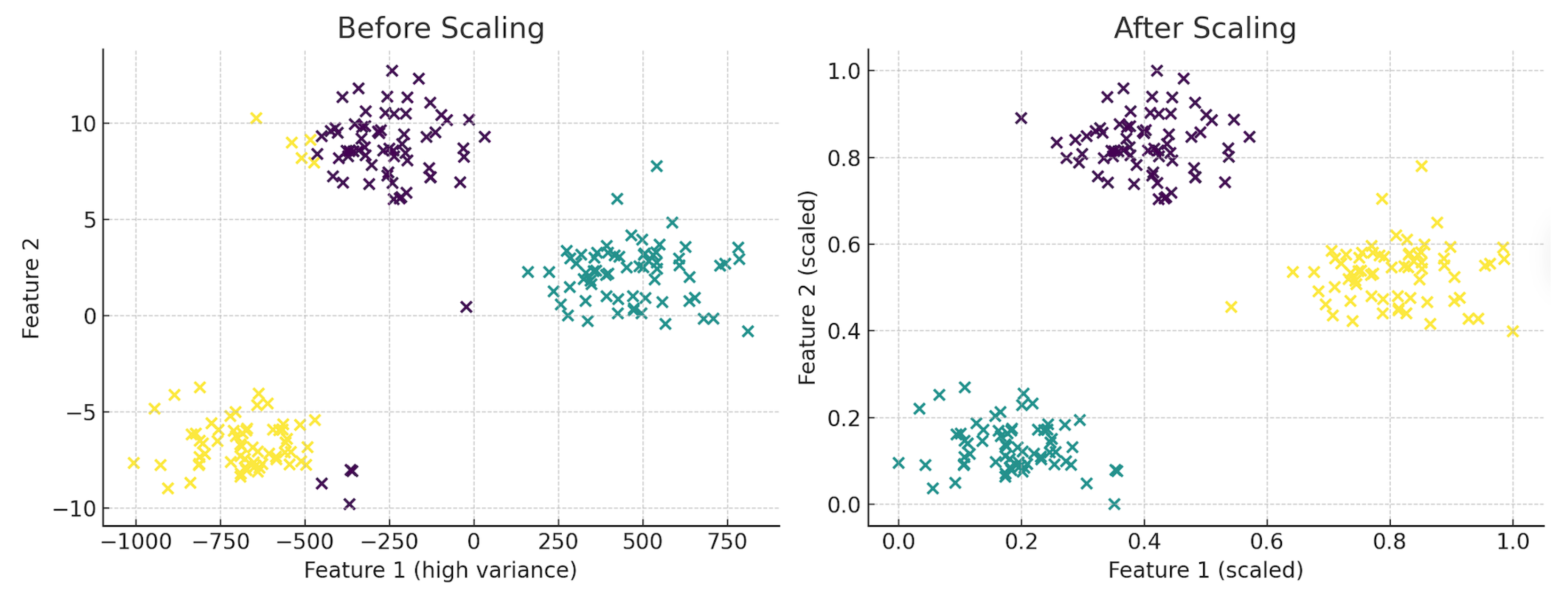
Many ML algorithms, especially those reliant on distance metrics or gradient descent, exhibit sensitivity to feature magnitudes. When input features possess varying scales, these algorithms may exhibit erratic behaviour or converge inadequately. Figure 3 demonstrates this effect utilising a synthetic dataset. In the absence of normalisation, clustering is skewed by feature imbalance, whereas min-max scaling facilitates precise cluster identification.

The choice of an appropriate scaling technique should be guided by the intrinsic properties of the dataset, as well as the particular properties of the mining algorithm being utilised. For example, decision tree-based algorithms like random forests and gradient boosting have a level of insensitivity to monotonic transformation, hence often dispensing with the need for scaling. However, models based on distance measures and NNs are well known to realise optimal performance when their features are scaled appropriately. In the case of multiple variables, the use of feature-based uniform scaling is imperative to avoid changes in patterns of correlation.

Finally, it is important for the scaling parameters to be computed only on the training set (or training folds within CV) and then applied to validation/test data to prevent leakage of distributional information [25,26]. In practice, this should be implemented within CV folds: scalers must be fitted only on the training fold and then applied to the validation/test fold. Even minor leakage of distributional statistics can inflate performance metrics and undermine generalisation [8,38]. This prevents contamination: even minor differences in test set statistics can bias coefficients and thresholds, inflating accuracy and undermining generalisation. This ensures that no statistical information from the test distribution contaminates the training process. Otherwise, even minor leakage can artificially inflate performance metrics and compromise generalisation [8,46].

Min–max scaling is highly sensitive to extreme values: a single outlier can compress the dynamic range of the remaining samples; in such cases, clipping winsorisation or a robust scaler (median/IQR) is preferable; z-score standardisation implicitly relies on roughly symmetric distributions; under heavy skew the mean/variance can be unrepresentative, in which case log/Box–Cox transforms or robust scaling provides more stable behaviour [2,6]. Tree-based models are largely insensitive to monotone transformations, but distance- and gradient-based learners usually benefit from consistent scaling across features [21,38,39,47]. In our taxonomy (Section 3), these scaling and transformation choices fall under Stage 2 (Transformation, see Figure 2), where the decision between simple or robust methods is guided by data distribution, interpretability, and robustness needs.

Why Fit Scalers Only on Training Data

Estimating scaling parameters (mean, variance; min, max; quantiles) on validation/test introduces information from held-out data and inflates performance estimates. Therefore, scalers must be fitted exclusively on the training portion (or training folds) and applied to validation/test without refitting [2,31]. Empirical studies show that the choice of normalisation alters both predictive performance and the set of selected features, with dataset-dependent effects [48,49].

3.4. Encoding Categorical Variables

To apply categorical variables to most DM models, it becomes necessary to represent these as numerical values. The choice of an encoding technique strongly impacts both the efficiency and interpretability of the model. One-hot encoding provides a common, simple technique to produce binary indicators of every distinct category [27]. Though this does not compromise any integrity of original categorical values and does not impose ordinal assumptions, its use on variables with too many distinct values can lead to increased dimensional feature spaces, thereby inflating memory usage and extending training times. Where cardinality is high, encoders that control dimensionality or application of rare-level grouping to avoid variance inflation are preferred [27].

Ordinal encoding assigns numerical values to categorical variables, thus creating a perceived ranking that might not reflect true relationships. Though more efficient in disk space usage than one-hot encoding, this approach risks causing algorithms to make incorrect assumptions that numerical differences imply semantic meaning [27]. For nominal variables with high cardinality, other strategies like target encoding, which replaces categories with the mean of the target variable, and frequency encoding, which uses the relative frequencies of each of the categories, are utilised [50]. Though these approaches can provide improved modelling effectiveness, they also share the risk of overfitting, especially when working with small sample data.

More sophisticated methods tackle the conversion of categorical variable representations into continuous vector representations by the application of deep learning methods. The entity embeddings learned in the training of NNs capture subtle interdependencies between categories and have the ability to represent high-dimensional spaces [51]. Such methods require large datasets and careful parameter tuning, and they can incidentally sacrifice interpretability due to the involved complexity. Methods using a hybrid model—using one-hot encoding for common categories while summing infrequent categories—can effectively balance expressiveness and generalisability. In fact, any coding frameworks must ultimately be aligned with goals related to task modelling, dataset size, and interpretability standards.

Choosing an appropriate encoding method for categorical variables is crucial for both model performance and interpretability. The choice depends on the data type, cardinality, and target task.

Table 4. Summary of categorical encoding techniques, including typical use cases, benefits, and challenges.

Encoding Method	Use Case	Pros	Cons
One-Hot Encoding	Low-cardinality nominal variables	Preserves category identity	High dimensionality
Ordinal Encoding	Ordinal variables	Compact, simple	Imposes artificial order
Target Encoding	Predictive categorical vars	Captures target signal	Leakage risk if misused
Frequency Encoding	High-cardinality nominals	Efficient, scalable	May inject bias
Entity Embeddings	Large, complex datasets	Learns deep representations	Hard to interpret

Target/frequency encoders should be applied with out-of-fold fitting and smoothing to avoid leakage and overfitting [2,27]; entity embeddings are powerful for high-cardinality features but require sufficient data and reduce transparency [51].

summarises widely used encoding techniques along with typical use cases, strengths, and potential pitfalls, helping practitioners balance expressiveness, scalability, and interpretability.

4. Feature Construction and Selection

This section discusses Stage 5 in Figure 1, where the pipeline’s attention now moves from input preparation to the build-up of representations that the model is supposed to learn. In this stage, either manual or automated processes generate features, often assisted by domain knowledge, and then are polished using filter, wrapper, or embedded selection methods to maximise signal strength, while minimising redundancy. The result is an improved and informative feature set that maximises interpretability and efficiency, thus supporting the DR highlighted in Section 5.

4.1. Manual vs. Automated Construction

Feature construction/generation/extraction refers to the process by which fresh features are created or existing features transformed to better capture intrinsic patterns within available data. Often, manual feature construction depends on the knowledge of domain experts, who invent new variables by combining, transforming, or aggregating raw feature attributes into a form pertinent to real-world objects or decision-making procedures.

For example, in an e-commerce dataset, manually constructed features might include “time since last purchase”, “mean order value”, or “category diversity” [52]. These carefully crafted features often represent subtle indicators to boost model performance beyond what simple model tuning can achieve. However, its construction process is subjective, manual, and can be problematic when it comes to scalability to different domains or datasets. Furthermore, it requires deep knowledge of data, as well as business context, which makes it less available to domain-unspecialised practitioners. Also, cognitive biases innate to human decision-making can lead to omission of crucial interactions or conversions.

Automated feature construction aims to mitigate these constraints by the systematic creation of potentially new features. One major such method is Deep Feature Synthesis (DFS), used in libraries such as Featuretools [28], tapping into the relationships found in relational data to generate features via aggregation and transformation operations [29]. The methodologies included also cover polynomial expansion, interaction discovery, and other unsupervised transformation techniques, like clustering-based encoding. AutoML frameworks often incorporate automated feature construction as part of their optimisation pipelines [53,54]. While these methods help improve scalability and reproducibility, they can unwittingly create redundant or suboptimal features, which need further filtering or selection steps. In reality, finding a balance between automated and manual feature construction typically proves to be the best approach.

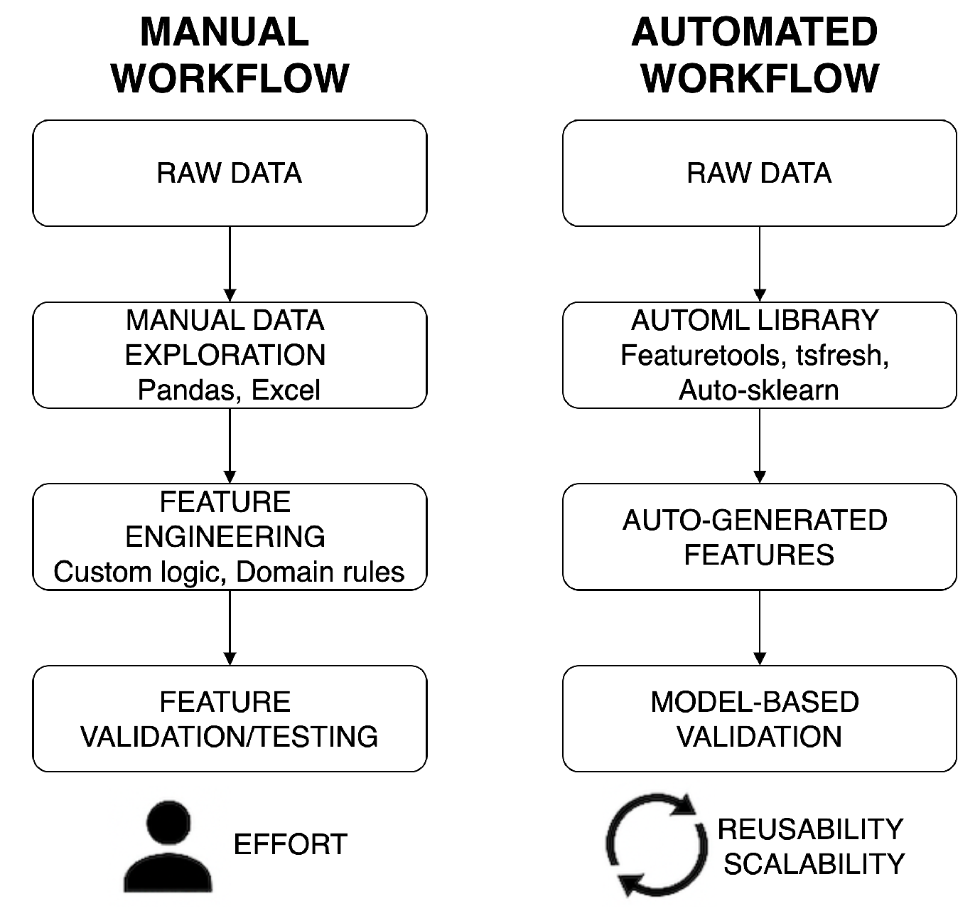
Therefore, the choice between manual and automated feature construction affects both development time and model generalisability. Manual workflows rely heavily on domain intuition, whereas automated approaches leverage scalable tools and heuristics. Figure 4 illustrates this comparison by outlining the different steps and toolchains involved in each workflow.

Decision Framework

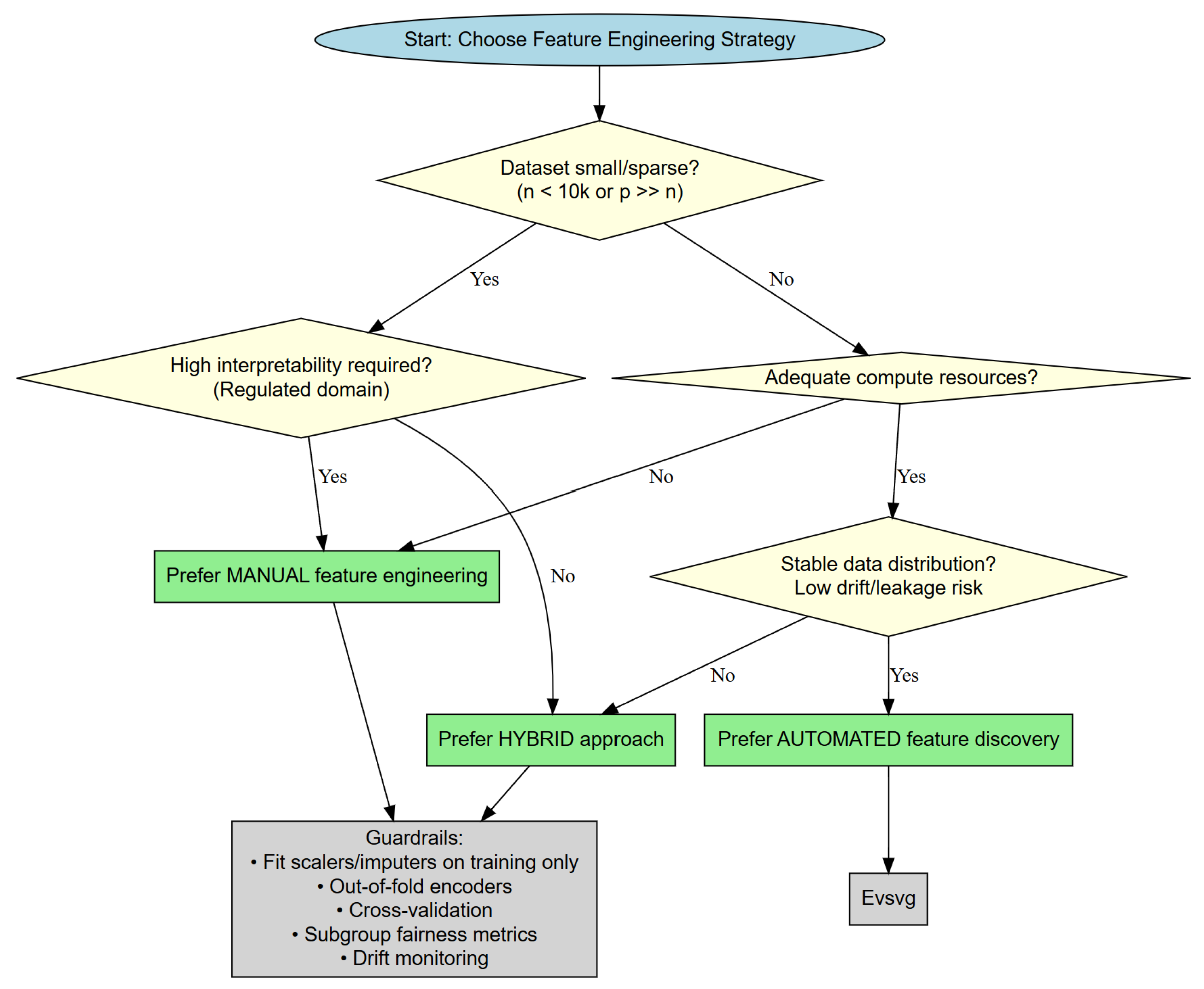
To make the decision between automated, manual, and hybridised feature engineering operable, we present a flowchart-like methodology (Figure 5). The framework works along four dimensions: (i) data scale and sparsity, (ii) interpretability and regulatory requirements, (iii) compute/time budget, and (iv) data stability and drift. Each one of the outcomes (manual, automated, or hybrid) is also aligned with guardrails: train-only fitting of imputers/scalers/encoders, out-of-fold encoders, in-fold CV, and subgroup fairness metrics. This framework expands upon the current conceptual taxonomy (Figure 2) into an actual, step-wise guide, explicitly outlining the trade-offs between dataset attributes, interpretability, resource usage, and stability, thus ensuring that the process is not just theory-informed but also practically translatable.

4.2. Domain-Driven Feature Creation

Domain knowledge can be an asset for feature engineering [52]. Professionals with such knowledge can often identify latent variables or structural relationships not apparent when only dealing with raw data. For example, in healthcare analytics, a domain expert might recommend feature construction to represent the co-occurrence of different symptoms or a composite health risk score from laboratory measurements. For marketing, features based upon domain knowledge could include customer lifetime value judgments, affinity scores showing product correlations, or seasonality correlations tied to buying behaviour.

Domain-informed feature engineering often supports temporal aggregation, including the computation of rolling averages, cumulative statistics, and lag variables in time-series datasets, to more effectively capture temporal dependencies and trends. In addition, the augmentation of base attributes by including external data sources can be useful [9,28,29,52]. For example, combining meteorological, geographical, or macroeconomic data. Creating aggregation hierarchies, including customer-level figures aggregated at regional or store levels, in normalised enterprise data can lead to gains in performance and understandability [55,56].

4.3. Filter, Wrapper, and Embedded Selection Methods

The increasing complexity and size of datasets have led to more available features, often more than what is practical or useful. Feature selection is essential in reducing dimensionality, enhancing the generalisability of models, and aiding interpretability. Feature selection techniques can be grouped into three main categories: filter, wrapper, and embedded methods [30,52,57].

Filter methods are notable for their model freedom and rely on statistical values to determine the importance of features relative to the target variable. The most widely used metrics include Pearson correlation, mutual information, Chi-square statistics, and ANOVA F-values [52,58]. These techniques are computationally inexpensive and can be applied before model training; however, they do not consider interactions between features or the specific learning algorithms used by the model.

Wrapper methods evaluate sets of features by training and testing a model for each respective set. A well-known example is Recursive Feature Elimination (RFE), which progressively removes the least relevant feature according to model performance [30]. Wrapper methods typically yield better results than filter methods, especially when feature interactions are important; however, they are computationally intensive and prone to overfitting, particularly with small datasets.

Embedded methods incorporate feature selection directly within model training (e.g., regularisation in Least Absolute Shrinkage and Selection Operator (LASSO)/Elastic Net, feature importance in decision trees). Regularisation procedures, including LASSO, or L1 regularisation, and Elastic Net, have the ability to automatically set the coefficients of unimportant features to zero. Tree-based models also generate statistics involving feature importance, aiding in informing selection procedures. Embedded methods often balance efficiency and effectiveness best, and when combined with simple filters in a pipeline, they achieve high performance at moderate cost [59].

Filter methods are computationally efficient, scaling almost linearly with the number of features, but they ignore feature interactions and can rank correlated variables inconsistently. Wrapper methods explicitly evaluate subsets and often achieve higher predictive performance, but they are orders of magnitude slower and prone to overfitting in high-dimensional or small-sample settings [30]. Embedded methods strike a middle ground: they integrate selection within model fitting, balancing efficiency with the ability to capture interactions, but their outputs are model-dependent and may not generalise well to other learners [59]. Thus, the choice of approach should be driven by dataset dimensionality, computational resources, and the intended downstream model.

Feature selection methods are commonly classified into filter, wrapper, and embedded methods, each offering distinct benefits and trade-offs depending on dataset size, modelling complexity, and performance goals.

Table 5. Comparison of filter, wrapper, and embedded feature selection methods across multiple dimensions.

Method	Examples	Model Dep.	Cost (Fits/CV)	Strengths	Limitations	Indicators
Filter	Corr., MI, ${\chi }^2$	Indep.	≈0 (stat-only)	Fast; interpretable; near-linear in p	Ignores interactions; unstable under collinearity	Stability across folds (e.g., Nogueira index) [60]; regime: very high p, limited compute.
Wrapper	RFE; Fwd/ Back sel.	Dep.	≈$k\times S$	Captures interactions; task-aligned	Expensive; overfitting risk in small-n	Report S, wall-time, nested CV status; stability across folds; ablation vs. filters/embedded.
Embedded	LASSO; Elastic Net; Trees	Dep.	≈$k\times 1$ per model	Integrated with model; balances cost/accuracy	Model-dependent selection; may not transfer	Coeff. sparsity/feature counts; stability across folds; regime: moderate/large n, structured p.

Cost proxy is the number of model fits per k-fold CV. For greedy RFE with step s, $S\approx p/s$ per CV run; beam/GA wrappers can raise S substantially. Always report k, S, wall-time, and whether nested CV was used. Stability should be reported via selection overlap or the Nogueira measure [60]. See also [30,59] for method families and trade-offs.

presents a comparative analysis of these three categories, outlining their operational characteristics, computational cost, and impact on modelling workflows.

4.4. Correlation, Mutual Information, and Variance Thresholds

Quantitative measures are often used to inform feature removal or selection based on their statistical properties. Correlation analysis can be used as a tool to identify redundant features defined by linear dependencies. Features that have a strong level of correlation (e.g., a Pearson measure larger than 0.9) can potentially lead to multicollinearity, undermining the stability and interpretability of linear models [52]. While sophisticated DR techniques, including PCA, can overcome this problem, more basic techniques, such as the removal of one of the highly correlated features, may be adequate.

Mutual information can be defined as a nonlinear measure of feature-target variable dependency. Unlike correlation, it can capture more complex dependency and has a special benefit when handling categorical features. Mutual information, however, can be sensitive to discretisation parameters and can potentially overestimate variable importance in noise-dominated datasets [58]. The use of statistical significance testing or permutation techniques can help to validate the resulting estimates from mutual information.

Functions exhibiting low variance, referring to minimal change across many observations, are found to be poor predictors and tend to be pruned using defined variance threshold criteria. The approach becomes very helpful when dealing with high-dimensional sparse data, particularly when such data originate from one-hot encoding techniques [52]. Nevertheless, one needs to be cautious, as sporadic values can have critical significance. For example, a binary variable created to indicate fraudulent transactions can have low variance but strong predictive ability. Typically, variance thresholds should be used after applying different filtering methods and always be tested against performance metrics. These statistics work together to develop an interpretable and well-informed feature set.

As a practical rule, zero-variance features can be removed completely and near-zero-variance predictors (e.g., frequency ratio >20:1 or unique value proportion <10%) reviewed using resampling frameworks. Arbitrary defaults such as 0.01 should not be adopted blindly. Thresholds should be tuned and validated against predictive performance [2]. Ultimately, feature selection and construction set the stage for the next step: reducing dimensionality of the feature space, which is discussed in Section 5.

In the context-aware taxonomy, these approaches belong to Stage 4 (Feature Selection, in Figure 2), where the key trade-off lies between computational cost, reliability to interactions, and model interpretability.

Interrelationship with DR

Feature selection/construction and DR are complementary rather than substitutive:

1.

When to prefer selection → reduction. If interpretability, regulatory traceability, or stable feature semantics are required, prune redundancy first (filters/embedded in Section 4.3 and Section 4.4) and apply DR thereafter to compress residual collinearity. This retains named features, while still curbing variance.

2.

When to prefer reduction → selection. In ultra-high-dimensional, sparse regimes (e.g., one-hot with many rare levels), apply a lightweight DR step (e.g., PCA or hashing-based sketches) to mitigate dimensionality, and then perform wrapper/embedded selection on the compressed representation.

3.

Order-of-operations ablation. Evaluate four candidates under the same CV split: (i) baseline, (ii) selection-only, (iii) DR-only, (iv) selection→DR, (v) DR→selection; pick the least-complex option that improves task metrics without harming calibration/stability.

4.

Guardrails. Fit every statistic within folds (selection criteria, DR components) and apply to hold-outs only; report component counts and selected features per fold. When DR reduces semantic transparency (e.g., neural embeddings), justify with performance/calibration gains and provide post hoc projections where possible.

5. DR Techniques

Beyond feature selection, another approach to handling high-dimensional data is DR. It seeks to project data into a lower-dimensional space, whilst preserving important structure. This section reviews both linear and nonlinear DR methods (Stage 6 in Figure 1).

5.1. Principal Component Analysis (PCA)

PCA represents a commonly used technique in performing linear DR, which projects high-dimensional data into a set of low-dimensional, orthogonal variables denoted by principal components. The components represent themselves as linear combinations of original features aiming to maximise variance residing within data. There are multiple usages of PCA: it reduces computational cost, reduces multicollinearity, and increases the ability to visualise high-dimensional data [61]. However, retaining a fixed percentage of variance (e.g., 90–95%) does not guarantee optimal predictive performance; the number of components should be chosen by cross-validated task metrics rather than a variance rule of thumb. PCA must be fitted on the training split only to avoid information leakage from the test set.

The mathematical principle behind PCA is Eigen decomposition or Singular Value Decomposition (SVD) of the covariance matrix computed from the input features [61]. The leading principal component corresponds to maximum variance, and the following principal component to the next maximum variance, orthogonal to the previous, and so forth. Selecting only the top k components, it becomes possible to retain much of a dataset’s structure and discard noise and redundancy. One common rule of thumb is to retain adequate components in such a way that, together, their variance captures around 90–95% of all variance; its value, however, may be domain-dependent.

PCA is particularly valuable for exploratory data analysis, where visualising data in two or three dimensions can reveal clusters, trends, or anomalies, which are not apparent in higher dimensions [61]. It also benefits algorithms sensitive to redundant or correlated features, such as k-means clustering or linear regression.

However, PCA works on an assumption of linearity and has sensitivity to data scale. In addition, principal components are linear mixtures without clear semantic meaning, which can limit interpretability in regulated or explanation-critical contexts [8,61]. As such, standardising input features prior to PCA application is required. Additionally, components resulting from PCA tend to be difficult to interpret, not necessarily mapping to the original feature space. This property can be problematic in cases where interpretability or regulatory compliance is needed. Regardless of these challenges, PCA remains a strong and flexible tool, best implemented in the early stages of data analysis or as a preprocessing step in more complex analysis.

5.2. Autoencoders and Neural Embeddings

Autoencoders form a special class of NN architecture aiming to draw useful representations from input data by leveraging unsupervised learning techniques [32]. These networks have two primary units: an encoder, which maps input to a representation in the latent space, and a decoder, which tries to reproduce the initial input from its encoded form. Optimising reconstruction error while training the encoder, the resultant network tends to converge to a low-dimensional representation of input data, which retains its most useful properties.

Unlike PCA, which can only deal with linear transformations, autoencoders have the ability to capture nonlinear associations, thus making them suitable for complex datasets in which linear projections cannot capture the underlying organisation [33]. Extensions like denoising autoencoders add strength by reconstructing pristine inputs from damaged ones, while Variational Autoencoders (VAEs) add probabilistic encoding and regularisation methods to encourage the construction of informative latent spaces [62].

Autoencoders have immense value in domains of image, text, or sensor data; moreover, they have been successfully used within structured tabular datasets. Their efficiency largely depends on multiple factors, such as architecture, activation functions, optimisation parameters, and training data level. Autoencoders of deep architecture, which have multiple hidden layers, perform very well in extracting hierarchical representations; however, they require large datasets and careful tuning to avoid overfitting. Applications as in [32,33] typically involve thousands of instances; in small-sample settings, they may underperform simpler linear methods unless strong regularisation (e.g., dropout, early stopping) is applied.

One of their main advantages is the latent embeddings they produce, which can be used as features for other subsequent tasks, such as classification, clustering, and outlier detection. These embeddings are usually representations of high-level abstractions and improve model generalisability. However, their very nature as black-box modules makes them difficult to interpret, thus making them less ideal for applications where feature translucency is important. However, they remain a very powerful nonlinear replacement for traditional dimension reduction methods and are a vital part of preprocessing modules in deep learning and DM pipelines.

5.3. Manifold Learning Methods

Manifold learning methods belong to nonlinear DR techniques used for uncovering the inherent geometrical structure of high-dimensional datasets. They rely on points within large-dimensional spaces, often located on or near a low-dimensional manifold embedded within a higher-dimensional setting. Through maintaining local or global geometrical attributes, they make it possible to project data from high-dimensional contexts to low-dimensional representations, whilst preserving crucial structural features.

t-SNE has been recognised for its utility as a DR algorithm well-suited for high-dimensional data, commonly reducing them to two or three dimensions for visualisation purposes [63]. t-SNE works by converting distances between points to joint probabilities, then lowering these probabilities to deduce the divergence between the original and the low-dimensional representations. t-SNE is most effective in retaining clusters and local patterns; however, it is not capable of retaining global structural relationships and is very sensitive to hyperparameters like perplexity and learning rate. Consequently, t-SNE is best treated as an exploratory visualisation tool rather than a stable feature transformer for predictive training; results can vary across runs and settings [63,64]. t-SNE also requires a great deal of computational power, and its non-parametric nature hinders it from generalising to new data without retraining.

The UMAP algorithm constitutes a novel technique distinguished by increased computational effectiveness, better global pattern retention, and a more varied set of parameters, promising prospective applications [65]. Despite an improved global structure, UMAP embeddings remain stochastic and hyperparameter-sensitive; report seeds and configuration; and avoid interpreting embedded distances as metric-faithful [65,66]. UMAP, in turn, creates a weighted k-nearest-neighbour graph inside high-dimensional spaces and adjustingly manipulates a low-dimensional representation to retain local associations concomitantly with some global correlations.

Such techniques remain best exploited in exploratory data analysis or visual investigation of complex datasets, such as gene expression profiles and word embeddings. Since most techniques remain chiefly used for visualisation within predictive modelling paradigms and not necessarily operating as feature transformers per se, their ability to reveal underlying structures incorporates critical benefits to preprocessing techniques. These techniques can be used to perform feature engineering, support noise identification, and improve clustering techniques. Interpretations, however, need to remain cautious, as distances measured in the low-dimensional representation cannot necessarily represent meaningful associations within the original dataset.

DR methods differ not only in their underlying assumptions, but also in how they reveal structure in complex datasets.

Table 6. Summary of DR methods and their practical trade-offs.

Method	Advantages	Limitations
PCA	Fast; reduces multicollinearity; variance-explained criterion	Linear; components hard to interpret; variance retention $\nRightarrow$ accuracy; fit on train only to avoid leakage
t-SNE	Reveals local clusters; strong for visualisation	Distorts global geometry; sensitive to hyperparameters and seeds; non-parametric (no out-of-sample mapping)
UMAP	Faster; often better global structure; flexible parameterisation	Stochastic; hyperparameter-sensitive; embedded distances not metric-faithful
Autoencoders	Nonlinear compression; scalable; denoising/variational variants	Data- and compute-demanding; tuning-sensitive; latent factors opaque

summarises practical trade-offs among PCA, manifold learning, and autoencoders to guide method selection in applied workflows.

Additionally, Figure 6 compares three widely used techniques: PCA, t-SNE, and VAE. PCA, being linear, captures global variance but may fail to separate nonlinearly distributed classes. In contrast, t-SNE and VAE are better suited for revealing compact, nonlinear clusters in latent space. VAE in particular produces a continuous yet separable embedding that resembles its generative modelling objective.

6. Preprocessing Pipelines and Automation Tools

6.1. Pipeline Design in Scikit-Learn and PyCaret

The creation of reliable and reproducible preprocessing pipelines forms a central component of modern DM and ML approaches (Stages 4–7 in Figure 1). Libraries like scikit-learn and PyCaret facilitate seamlessly integrating preprocessing operations into every step of model creation and assessment, thereby ensuring consistency across process components [31,67].

In the scikit-learn library, the ColumnTransformer and Pipeline objects are essential parts [31]. Pipeline enables the definition of a pipeline of transformations, such as imputation, scaling, and encoding, before applying a ML estimator. This framework ensures all preprocessing steps are performed systematically. On the other hand, ColumnTransformer enables the implementation of different preprocessing methods on different subsets of features; it can be used, for example, to apply scaling to numerical columns while performing, at the same time, one-hot encoding on categorical variables, allowing, therefore, a more flexible construction of modular pipelines, better suited to handling data heterogeneity efficiently. In addition, it makes it possible to perform hyperparameter tuning by grid or randomised search procedures, which can be used on extensive pipeline configurations instead of single models alone.

Figure 7 visualises such a pipeline using a ColumnTransformer to separately scale numerical data and encode categorical data before passing the result on to a classifier.

PyCaret expands on the capabilities of scikit-learn by the inclusion of a low-code application programming interface, which automates several parts of the preprocessing pipeline [67]. Upon importing a dataset into PyCaret, it automatically performs several preprocessing operations, such as imputation, feature scaling, encoding, outlier detection, transformation, and feature selection. Such automation allows entry into the market for beginners, while providing experienced practitioners with room for customisation. It also accommodates experiment logging, model comparison, and ensemble building, making it an invaluable resource in both research and production environments.

Another benefit of pipeline architectures is their ability to prevent data leakage; all transformation parameters, including scaling factors and means, are calculated from the training set before their application to the test set. Additionally, they improve the efficiency in model deployment by bundling the model and its relevant transformations into a single versioned object, which can be retained and reused. In this regard, modularity becomes highly advantageous in system development, which requires maintainability and scalability, especially in production environments, where reliability and traceability are important. By bundling its related transformations with a model into a single versioned object, they further enhance the productivity in model deployment.

6.2. DataPrep, Featuretools, and Automated Feature Engineering (AutoFE)

Whilst scikit-learn and PyCaret provide generalisable preprocessing pipelines, some specialist tools focus on automating specific aspects relevant to feature engineering and data preparation. Examples of specialist tools include DataPrep, Featuretools, and some newer libraries created for AutoFE.

DataPrep is a Python library intended to make exploratory data analysis and cleaning easier [68]. It provides sophisticated functionality for normalising column names, standardising date format, filling missing values, and detecting outliers. Additionally, its visual analytical features, such as distributions, correlation matrices, and null heatmaps, help gain insights into data quality before model building commences. Compared to more comprehensive frameworks, DataPrep is distinguished by its lightweight approach and focus on the rapid generation of insights, making it highly useful during the initial stages of DM.

Featuretools is a leading application of DFS, a framework that aims to automatically derive new features from relational data structures [28]. By analysing the relationships between tables (e.g., transactions and customers), it creates compound features like “average purchase amount per customer” or “total distinct items purchased last month”. Featuretools is best when applied to normalised schemas or temporal hierarchies, providing the capability to generate hundreds to thousands of possible features with little or no manual work. Further, its ability to perform large-scale computations by utilising Dask and Spark allows it to execute large-scale analytical workflows with high efficiency.

Automated feature engineering software, such as autofeat, tsfresh, and ExploreKit, promote automation by the use of statistical heuristics, information theory-based principles, or domain-specialised search techniques, which allow for the detection or identification of strongly significant features [29,54]. The tools normally support numerical and categorical data inputs, and they can suggest nonlinear transforms, interactions, and heuristics based on domain-relevant expertise. Also, some AutoML frameworks integrate AutoFE into their search process, allowing for end-to-end optimisation of features and models. Automation has some definite strengths like scalability and consistency, but it also has some pitfalls, such as feature proliferation, loss of interpretability, and risk of overfitting. Thus, AutoFE needs to be complemented by post-processing and validation methods to guarantee that the created features promote improved model performance while meeting the task’s objectives.

6.3. Pipeline Serialisation and Reproducibility

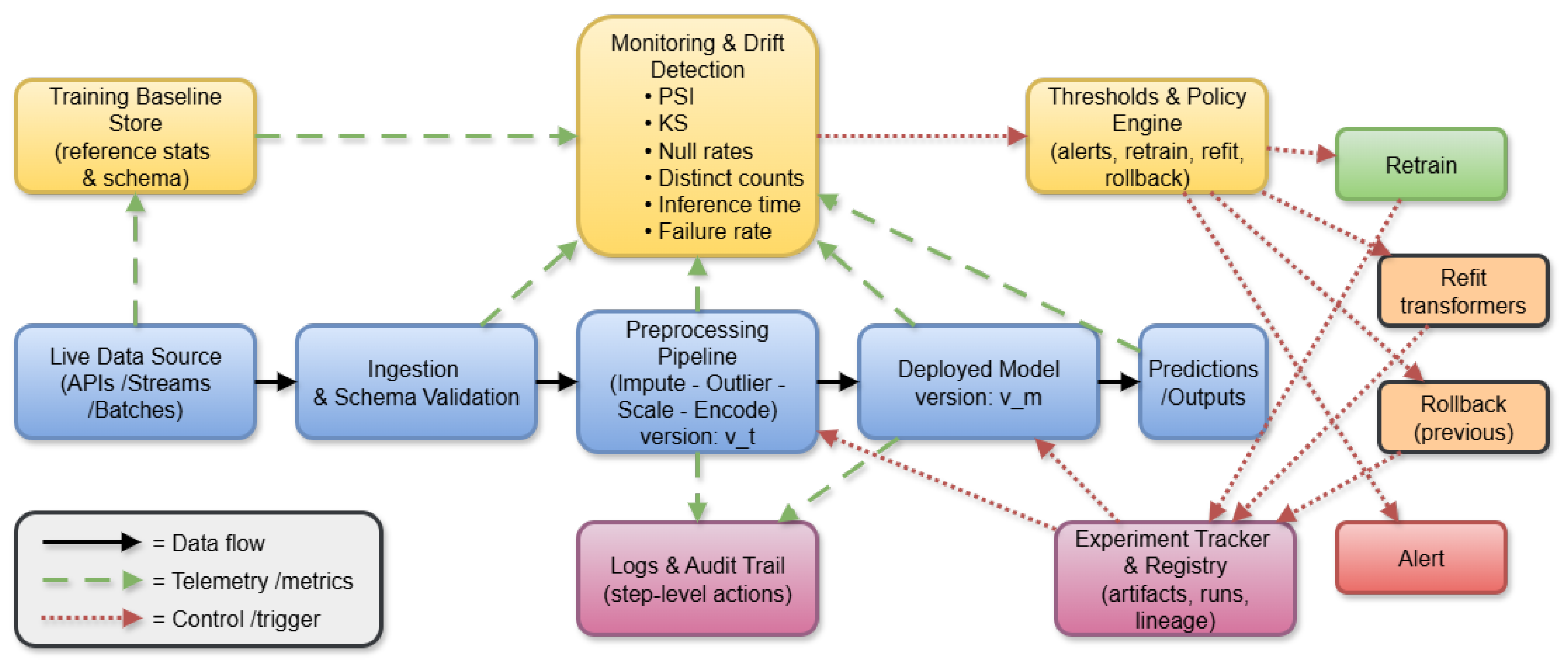
A core property of effective DM infrastructures is reproducibility. Preprocessing pipelines deserve special consideration, since inconsistencies in the training or prediction stages can reduce model effectiveness or produce unexpected outcomes (see Section 9.7 for the placement of experiment tracking and versioned redeployments).

Serialisation permits saving a trained pipeline, including all preprocessing components within a model, in a form amenable to later loading. In Python, commonly used tools for performing serialisation are joblib and pickle; similar functionality exists in most frameworks and programming languages. For extending the practical usefulness of deep learning and to support cross-platform deployments, Open Neural Network Exchange (ONNX) provides a format to perform the serialisation of pipelines, focusing on portability and shareability.

The reproducibility promotion is intrinsically supported by following systematic definitions of pipelines, the use of configuration files (e.g., formatted in YAML or JSON), and the application of version control software. The clear delimitation of transformation parameters (such as imputation methods, scaling, or chosen features) in a separate configuration file, for instance, supports pipeline execution on different data subsets or on different computers with one command. Additionally, the use of software tools such as MLflow, Data Version Control (DVC), or Weights & Biases further supports experiment tracking, artefact preservation, and change analysis in pipelines for different iterations [69].

A basic additional requirement is schema consistency. Data processing models need to include mechanisms for ensuring the consistency of incoming data with predetermined formats, column descriptions, and statistical distributions. These steps considerably reduce the risk of experiencing runtime faults or hidden failures at the implementation level. In cases where reproducibility is of high priority, such as financial forecasting or medical assessments, identical results across these approaches trigger concerns around compliance with regulatory needs, thus emphasising the imperatives of transparency and accountability. Finally, the use of reproducibility and serialisation methods is crucial for improving the scalability and reliability of DM systems. Such approaches enable seamless deployment and monitoring of models, promote collaboration, aid debugging, and help to ensure long-term sustainability of analysis endeavours.

7. Evaluation of Preprocessing Impact

7.1. Measuring Improvements in Model Accuracy and Stability

Comparing the effectiveness of preprocessing operations is important for understanding their true impact on model performance and ensuring that improvements observed are not a result of random fluctuations or intrinsic properties of the dataset [8]. One common method for comparative assessment is comparative modelling, which involves training a particular ML algorithm and evaluating it with and without a chosen preprocessing operation. Afterwards, differences in performance are measured based on different metrics, such as accuracy, precision, recall, F1-score, or Root Mean Square Error (RMSE).

To push beyond simple point estimates, professionals commonly use k-fold CV to assess how preprocessing’s effects generalise to different data subsets by measuring performance [44]. Such a technique works well to control variance and prevent overfitting, particularly when sample sizes are small. In such cases, improvements in preprocessing should not be evident from a single train–test split, yet they tend to become obvious when averaged across multiple folds.

Besides predictive accuracy, stability is a key consideration. A preprocessing pipeline that improves the model accuracy but produces significant variation across different validation folds might not be the best for deployment. Model stability can be measured by the standard deviation of performance metrics across different folds or by exploring feature importance consistency across models [60].

Other preprocessing methods, such as scaling and imputation, have a bidirectional effect on both the model accuracy and the interpretation and weighting of input features for models. Imputation refers to handling missing values, necessary before using certain models that, by nature, do not support NaN values (e.g., logistic regression) for the training process. Figure 8 shows the absolute coefficients from a logistic regression model, which was solely trained using imputed data, compared to data that was imputed after scaling. Due to logistic regression’s vulnerability towards feature scaling variability, this demonstrates how imputation changes feature importance, thus validating the statement that even simple preprocessing notably affects a model’s internal representation.

The effectiveness of preprocessing procedures can be evaluated indirectly by tracking increases in convergence rates, training times, or resource utilisation efficiency [30]. For instance, although accuracy will not be increased by normalisation or DR, it can reduce computational costs considerably or allow more complex models to be trained within set time constraints. Additionally, visualisation tools, like learning curves or confusion matrices, can be used to gain insight into how preprocessing decisions impact error distributions and general model effectiveness.

Above all, the argument in support of picking particular preprocessing methods has to be grounded in the application of performance metrics, stability tests, and interpretability assessments. Methods like ablation studies can be used, in which elements can be progressively removed from a preprocessing pipeline to estimate individual element contributions. In this comprehensive assessment framework, preprocessing cannot be treated as a black box; instead, it supports DM pipelines by allowing for more awareness, reproducibility, and ruggedness.

7.2. Bias–Variance Implications

The choice of preprocessing procedures has a strong impact on the bias–variance trade-off underlying generalisable predictive models. Bias has been defined as error due to very simple representations of the model, while variance represents error due to increased sensitivity of the model to slight variations in the training set. Certain preprocessing procedures would decrease bias simultaneously while variance increases, and vice versa, thereby requiring comprehension of their combined effects.

The feature selection process, for instance, can significantly reduce variance by eliminating noisy or collinear features, which tend to lead to overfitting on the training data [70]. On the other hand, too aggressive selection methods can add bias by eliminating informative features that are weak in signal. Similarly, outlier removal often reduces variance by removing extreme data points that play a significant role in model parametrisation. However, in real-world applications, like fraud detection or disease diagnosis, such outliers can represent infrequent yet significant cases, and removing them can increase bias by degrading the model’s capability to detect important edge cases.

Normalisation and scaling methods can improve the convergence reliability of gradient-based methods, later reducing model variance [71]. However, if normalisation distorts feature distributions or hides domain semantics, it effectively adds bias. When used carefully, DR techniques, like PCA, can reduce both bias and variance; however, blind adoption of such techniques can lead to the loss of important information.

To estimate such trade-offs, practitioners often use learning curves describing the behaviour of training and validation performance versus sample size [72]. Preprocessing techniques highlighting generalisable data should have a low generalisation error across the whole curve. In addition, special techniques, such as regularisation, can be combined with preprocessing to explicitly trade bias and variance and thereby reduce negative consequences from data preparation. In short, bias–variance trade-off assessment requires simultaneous empirical exploration, as well as deep knowledge of the application domain pertinent to a problem. Simply measuring mean accuracy cannot suffice; it becomes critical to consider consistency, fairness, and interpretability of model behaviour in different subgroups and settings. Thus, preprocessing cannot be treated as a static process, but rather as a set of tunable choices considerably affecting underlying learning dynamics.

• Protocol (controlling confounders).

To isolate the effect of a single preprocessing step (e.g., feature selection), imputation, encoding, scaling, and the downstream model/hyperparameters are held fixed; only the focal step varies across candidate settings. Evaluation uses nested or repeated k-fold CV, and results are reported as fold-wise mean ± SD. Learning curves (train/validation performance vs. sample size) are produced within the same splits to diagnose bias–variance behaviour. An ablation study removes or replaces the focal step to confirm the necessity. Reporting includes calibration (Brier score/ECE), selection or transformation stability across folds, and—where applicable—subgroup fairness metrics (see Section 9.3 for a general evaluation checklist).

7.3. Interaction with Downstream Mining Tasks

Different DM tasks have different responses to preprocessing techniques. What improves the effectiveness of one task can compromise performance in another, so task-specific evaluation becomes necessary at preprocessing workflow construction times.

For instance, normalisation is critical for distance-based models like k-NN or k-means clustering, where unscaled features dominate distance calculations and lead to skewed clusters or nearest neighbours [73]. However, for tree-based models, normalisation often has a negligible impact, as these models are scale-invariant. Applying unnecessary normalisation in such cases adds complexity without benefit and can sometimes interfere with interpretability.

Similarly, DR by procedures like PCA or autoencoders can enable clustering or visualisations by discovering latent group structures, but it can compromise interpretable relationships needed to support rule mining or feature attribution [63]. In association rule mining, where detection of presence or absence of specific categorical items plays a significant role, encoding protocols should preserve discrete semantics; too much feature merging to eliminate cardinality could lead to vital co-occurrence patterns becoming lost [74].

In classification and regression, it is critical that feature encoding and imputation of missing values be aligned to the predictive target. For example, target encoding uses response variable-based information and runs a risk of leakage if not properly implemented within a cross-validated framework [50]. For preprocessing within time-series analysis, it has to honour temporal ordering to avoid look-ahead bias, and this requires the application of special-purpose imputation and data splitting techniques.

The evaluation of preprocessing effectiveness should, thus, include not only traditional measures, but also goals related to particular tasks, e.g., clustering quality (e.g., silhouette score), comprehensibility (e.g., rule lengths), and critical business performance measures (e.g., false negative rate in fraud prevention). Suggested approaches include the creation of dual pipelines tailored for different tasks and methodical comparisons of outcomes in a structured and transparent framework.

8. Open-Source Libraries and Frameworks

The development of the open-source preprocessing ecosystem has led to the appearance of three closely related categories that support data preprocessing at different abstraction levels: (i) general-purpose ML libraries, providing explicit, composable transformers and pipelines (e.g., scikit-learn, PyCaret, and MLJ); (ii) AutoML systems concurrently searching for preprocessing choices and model hyperparameters, such as H2O AutoML, auto-sklearn, and Tree-based Pipeline Optimisation Tool (TPOT); (iii) notebook-based experimental ecosystems improving exploratory analysis, reporting, and reproducibility (demonstrated by Jupyter, featuring profiling, tracking, and versioning extensions). A quick comparison of such representative tools is presented in

Table 7. Comparison of representative open-source tools for preprocessing and experimentation. As this table is descriptive, software/tool versions are not fixed; capabilities have been stable across recent releases.

Tool	Category	Key Preprocessing/Pipeline Features	Best for
scikit-learn	Library (Python)	Composable transformers; Pipeline ColumnTransformer; CV with Grid/RandomisedSearch	Tunable, explicit workflows; benchmarking baselines
PyCaret	Low-code library (Python)	Auto setup (scaling, encoding, outliers, transforms); pipeline export; experiment logging	Rapid prototyping and quick model comparison
MLJ	Library (Julia)	Type-safe pipelines; unified interfaces; broad data-type support	High-performance Julia-native projects
H2O AutoML	AutoML	Auto imputation/encoding/scaling; ensemble search	Hands-off model + preprocess search at scale
auto-sklearn	AutoML (Python)	Joint search over preprocessing and model hyperparameters; meta-learning warm starts	Automated pipeline selection in the scikit-learn ecosystem
TPOT	AutoML (evolutionary)	Evolves DAG pipelines combining preprocessors and models	Discovering novel operator combinations
Jupyter + add-ons	Notebook workflow	Interactive EDA/reporting; parameterised notebooks; tracking and versioning (Papermill, DVC, MLflow)	Exploratory analysis and reproducible pipelines

. In addition, in the following subsections, each category is placed in the broader context, explaining the trade-offs concerning automation control and integrating them into the end-to-end pipelines described in Section 6.

8.1. Scikit-Learn, PyCaret, and MLJ

Several open-source libraries have evolved to be critical tools for data preprocessing, offering distinctive functionalities and conceptual paradigms. Representative libraries include scikit-learn (a general-purpose Python ML library), PyCaret (a Python low-code library that builds on scikit-learn and other frameworks), and ML in Julia (MLJ—a ML framework for the Julia language). As introduced earlier in Section 6, scikit-learn and PyCaret provide core preprocessing functionality. Here, we compare these with another framework, MLJ, highlighting unique features.

Scikit-learn represents the standard benchmark in the Python programming framework for general-purpose ML applications [31]. Its preprocessing module provides a comprehensive set of tools, ranging from imputers created to deal with missing data to standard, min-max, and robust scalers; encoders conceived to tackle categorical variables; and transformers to support polynomial feature expansion or normalisation procedures. Pipeline and ColumnTransformer classes support modular preprocessing, allowing users to design, prepare, and execute reproducible workflows defined by homogeneous transformation behaviour. Scikit-learn focuses on user-friendliness and composability, supporting seamless collaboration with models, CV procedures, and hyperparameter tuning by GridSearchCV or RandomisedSearchCV.

PyCaret is essentially rooted in the scikit-learn library and further integrates several other libraries, including LightGBM and XGBoost, to allow for a high-level abstraction to encourage rapid development processes [67]. One of PyCaret’s prominent features is the ability to automate preprocessing operations, which include outlier removal, feature scaling, encoding, application of transformation methods (like log and Box-Cox transformations), and multicollinearity checks. These operations are automatically performed when users set up a modelling environment using a single instruction. In addition, PyCaret supports logging experiments, measures models based on varied performance metrics, and performs exportation of detailed pipelines to production environments. This capability is especially beneficial in scenarios where the focus is laid on efficiency and reproducibility over detail-oriented handling of individual preprocessing operations.

In the Julia community of developers, the MLJ package provides a strong foundation for data preprocessing and for modelling operations [75]. Inspired by scikit-learn, MLJ creates type-safe pipelines, presents unified interfaces for data conversion and modelling, and supports a wide variety of data types. The inherent performance benefits of using Julia make MLJ particularly valuable in high-volume applications. In addition, MLJ is highly extensible, and developers can integrate custom preprocessing steps or use pre-trained models that exist in other Julia packages.

All of these libraries reflect a balance between automation and control. Scikit-learn is best suited for programmers who prefer in-depth, tunable workflows, while PyCaret is suited for practitioners who want quick results with minimal setup. MLJ offers a strong alternative for situations where performance matters the most or in research. All three provide the core foundation on which most modern preprocessing techniques are built.

8.2. AutoML Integration Tools

The arrival of Automated ML has prompted the development of tools that embed preprocessing within the frameworks of procedures at the stage of model selection and hyperparameter tuning workflows. These tools allow for automatic search through some preprocessing alternatives, such as encoding, feature selection, and normalisation, and consider a variety of algorithms, hence aiding inexperienced users to assemble functional models with little manual intervention.

H2O AutoML is an enterprise-grade platform supporting both cloud and on-premise environments. It automatically handles missing data, performs one-hot encoding, applies scaling where necessary, and runs a suite of models—including ensembles—to find optimal pipelines. Its preprocessing choices are guided by heuristics and domain-agnostic principles, ensuring general applicability across use cases.

Auto-sklearn, based on scikit-learn, augments the typical workflow of ML by applying Bayesian search to combinations of preprocessing and modelling by exploiting performance history to focus search on promising configurations using meta-learning techniques to initiate search from prior experimental outcomes [76]. Auto-sklearn possesses an interesting module in pipeline construction, which simultaneously explores transformation (e.g., standardisation and PCA) and encoding schemes, as well as model hyperparameters, thereby guaranteeing all-inclusive optimisation across the workflow.

TPOT utilises genetic programming techniques to discover and improve ML pipelines [77]. TPOT builds and repeatedly refines such pipelines as directed acyclic graphs, where nodes correspond to preprocessing operators or models. TPOT finds and changes pipelines across many generations to maximise a specified scoring function. Compared to grid or random search methods, this evolutionary method has the potential to find novel and effective preprocessing and modelling process combinations.

AutoML tools reduce manual intervention to a minimum; however, some challenges also accompany them. The black box nature of resulting pipelines can hinder interpretability, and the corresponding computational cost can be significant when searching large configuration spaces. Nevertheless, in prototyping, benchmarking, or deadline-constrained scenarios, AutoML tools represent strong substitutes to pipelines manually assembled. They also encourage best practices, such as training–validation splits, leakage avoidance, and logging of performance, which are natively implemented within their pipelines.

8.3. Jupyter Workflows and Experimentation Environments

Jupyter Notebooks are considered one of the most preferred tools for debugging and constructing preprocessing pipelines. Its interactive nature enables meticulous analysis of data, as well as probing distributions, inspecting transformations, and refining conceptualisations by adopting a feedback-rich mode of operation. Additionally, its ability to allow markdown functionality, produce detail-rich outputs, and easily coexist with libraries such as Pandas, Matplotlib, and Seaborn makes it an extremely valuable tool to perform exploratory data analysis.

Within its environment, data preprocessing can be improved considerably by exploiting specialist tools. Pandas Profiling works to produce detailed reports on data completeness, data type distributions, inter-variable correlations, and data quality issues, all within a single command [78]. Sweetviz provides comparative visual analysis based on training and testing datasets, focusing on feature distributions and correlations of these distributional features based on their relationship to the target variable [79]. Also, DataPrep.EDA provides similar functionality and can be easily implemented within pandas pipelines [68].

To improve reproducibility, abstraction mechanisms like Papermill reduce the complexities involved in running parameterised notebooks, thus acting as flexible template pipelines, which can be used with multiple datasets or experimental setups. Additionally, software packages like DVC [80] and MLflow [81] add experiment tracking, data versioning, and model registration capabilities, which enhance the monitoring and sharing of preprocessing pipelines dramatically [82,83] (see the registry and lineage linkages in Figure 9). These tools allow practitioners to save preprocessing parameters, annotate metrics, and track model artefacts, all within the Jupyter notebook environment.

Notebooks, handicapped by their restricted functionality due to a stateful execution environment, form a central element within scenarios where exploration and documentation are essential. There are many users who work through the process via Jupyter before moving to more advanced pipeline or scripting platforms, like Airflow and Prefect, when projects grow in size. Ecosystems around notebook extension and integration libraries can be interpreted as an effort to bridge interactive development and production pipelines so as to further establish a crucial role of notebooks within a preprocessing pipeline.

9. Best Practices and Design Patterns

9.1. Data Splitting and Leakage Control

Rigorous data partitioning is the cornerstone of reproducible pipelines. All transformations must be fitted exclusively on the training portion and then applied to validation and test sets to prevent information leakage [2]. This principle extends to imputation, encoding, scaling, and feature selection. Randomised k-fold CV [44] or stratified sampling should be applied for balanced estimates, while blocked or forward-chaining schemes are required for time-series data to avoid look-ahead bias [55]. Target-dependent encodings must be performed with out-of-fold or nested CV to eliminate label leakage [50].

9.2. Preprocessing Order

The order of operations determines pipeline validity. The recommended sequence is as follows:

1.

Data cleaning (error detection, type correction);

2.

Missing-value imputation;

3.

Categorical encoding;

4.

Scaling/normalisation;

5.

Feature construction;

6.

Feature selection;

7.

Model training.

Figure 10 summarises the canonical, leakage-safe ordering, emphasising that all data-dependent statistics are learned exclusively on the training partitions and applied downstream.

This canonical flow is supported by [1,73]. Imputation must precede encoding, since encoders cannot process missing values reliably, while scaling parameters must be fitted after imputation and encoding to avoid bias [31]. Tree ensembles are invariant to monotonic transformations, but linear and distance-based models require strict scaling [73]. The use of pipeline abstractions such as scikit-learn’s Pipeline ensures reproducibility and deterministic ordering.

9.3. Evaluation Protocols and Ablation

Evaluation should quantify both accuracy and stability. Nested CV is the gold standard for hyperparameter and preprocessing selection. Repeated k-fold CV provides variance estimates, reducing dependency on a single split [44]. Ablation studies systematically remove or substitute preprocessing steps, measuring their impact on predictive performance and variance [30]. Stability analysis of selected features across folds has been shown to indicate robustness [60]. Beyond accuracy, calibration and ROC-AUC should be reported to ensure that preprocessing choices align with the domain goals [73,84].

Table 8. Checklist for evaluation of preprocessing pipelines.

Protocol	Requirement	Rationale
CV	k-fold or nested CV	Reduces variance of performance estimates [44]
Leakage checks	Fit transforms on training folds only	Prevents optimistic bias [2]
Ablation studies	Systematic removal/replacement	Identifies contribution of each preprocessing step [30]
Stability metrics	Feature overlap across folds	Ensures robustness of selection [60]
Task-specific metrics	ROC-AUC, calibration error	Aligns evaluation with application objectives ([84])

showcases a checklist for evaluating preprocessing pipelines.

9.4. Logging and Reproducibility

Reproducibility requires the systematic documentation of preprocessing transformations and their parameters. Each step should produce metadata, including imputation statistics (e.g., number and proportion of missing values replaced), scaling parameters (means, variances, quantiles), and categorical encoding mappings. This information must be versioned alongside datasets and model artefacts to enable a full reconstruction of experiments [68].

Figure 11 depicts a provenance-centric logging schema linking raw data, fitted transformer parameters, experiments, and artefacts for auditable reruns.

Experiment-tracking frameworks such as MLflow [69] and DVC [80] provide mechanisms for recording preprocessing configurations and results. Provenance tracking, which maintains links between raw data, intermediate transformations, and outputs has been highlighted as an essential governance requirement [83]. Such practices ensure scientific reproducibility and build trust in ML deployments. Evidence of pervasive leakage further motivates fold-aware pipelines with strict train-only fitting and artefact versioning [14].

9.5. Fairness and Transparency

Preprocessing is not a neutral act: imputation, scaling, and encoding choices can disproportionately affect underrepresented groups. For example, imputing mean values may systematically bias minority populations, and high-cardinality encodings can embed hidden disparities [5,34].

Transparent encodings such as one-hot or ordinal are preferable when interpretability is a priority [31]. Advanced methods such as target encoding must be applied with out-of-fold fitting to avoid leakage and overfitting [27]. Entity embeddings can capture complex latent relationships [51], but they reduce transparency and require substantial data resources.

Fairness-aware preprocessing techniques, such as reweighting or sampling to reduce disparate impact, have demonstrated effectiveness in addressing bias [85]. Moreover, documenting feature inclusion/exclusion decisions and transformation rationales is a best practice for accountability and governance [5].

Table 9. Fairness and transparency checklist for preprocessing.

Area	Best Practice	References
Imputation	Assess subgroup bias before replacement	[7,18,35]
Encoding	Use out-of-fold fitting for target encoding	[27]
Transparency	Prefer interpretable encodings when feasible	[31]
Bias mitigation	Apply reweighting or resampling	[85]
Documentation	Log inclusion/exclusion rationale	[5,34]

provides a concise reference for fairness-aware preprocessing.

9.6. Automation Trade-Offs

Automated ML (AutoML) and feature engineering (AutoFE) systems can accelerate pipeline design, but they introduce trade-offs between performance, interpretability, and computational cost. Systems such as auto-sklearn [76] and TPOT [77] optimise preprocessing and modelling jointly, while PyCaret simplifies pipeline prototyping [67]. These frameworks often achieve competitive performance but may generate pipelines that are difficult to interpret, replicate, or maintain [12,54]. For production, AutoML outputs should serve as baselines that are simplified and refined manually. The key trade-offs of automated preprocessing systems are summarised in

Table 10. Trade-offs of automated preprocessing systems.

System	Strengths	Limitations
auto-sklearn	Joint optimisation of pipeline and model	Complex, less transparent [76]
TPOT	Genetic programming for pipeline search	Can produce bloated pipelines [77]
PyCaret	Low-code prototyping, fast deployment	Limited flexibility for advanced tuning [67]
AutoFE methods	Automated feature construction	Harder to interpret and validate [12,54]

.

9.7. Monitoring and Drift Response

In real-world deployments, preprocessing pipelines must adapt to evolving data distributions. Distributional drift can be detected with statistical methods, such as the population stability index or Kolmogorov–Smirnov test [86]. Once drift is detected, frameworks, such as those described by [86,87], can trigger retraining, recalibration, or alerting. Monitoring platforms like Deepchecks and WhyLabs provide practical implementations of these principles, integrating detection, alerting, and retraining workflows [87,88].

Figure 9 summarises the drift-monitoring architecture and its feedback loop from monitoring to policy and back to redeployment.

10. Challenges and Future Directions

The real-world application highlights three dynamic spaces in which preprocessing improvements must be ongoing: making large and varied datasets manageable; ensuring fairness, interpretability, and compliance with regulatory requirements; and responding to distribution shifts and goals. This section describes the main challenges and the most promising directions, including distributed, schema-aware tools; explainable, auditable, and ethically informed transformations; and adaptive, policy-based pipelines with the ability to self-correct and assess. Taken together, these developments reshape preprocessing from fixed scripts into robust, accountable infrastructures.

10.1. Scalability in Large and Heterogeneous Datasets

With datasets increasing in size, velocity, and variety, traditional preprocessing methods are faced with significant challenges of scalability [89]. High-dimensional attributes, mixed data types, and real-time data requirements call for new methods to be developed to solve the limitations of classical in-memory data processing paradigms.

In large-scale business or web-based deployments, the amount of data often exceeds the memory of a single machine, making the use of distributed computing unavoidable. Although libraries like Dask, Spark, and Ray make parallelised preprocessing easier, most of the preprocessing libraries (particularly those written in Python), are inherently single-threaded-friendly and memory-bound. Adapting these libraries to support distributed processing pipelines is very challenging, especially for operations like imputation or encoding, which are purely based on detailed data statistics across the entire process.

The second aspect of scalability relates to heterogeneity. Modern programs have to deal with structured, semi-structured, and unstructured data, including different types of log, transactional databases, sensor streams, and text data. Creation of preprocessing pipelines from a single source to support many modalities poses major challenges, especially in cases where schemas experience transformations over lengthy periods or when preprocessing jobs have complex, hierarchical dependencies.

To successfully tackle such challenges, future research activities should focus on developing scalable and schema-aware preprocessing frameworks that enable streaming execution, versioning of data, and module deployment strategies. Additionally, the use of lighter and resource-aware transformers, combined with the setting up of containerised microservices for the deployment of preprocessing applications, can help increase flexibility and encourage fault tolerance in production environments [90,91].

10.2. Fairness, Explainability, and Ethical Considerations

As data-driven models increasingly inform pivotal choices, such as loan decisions, hiring screenings, and health diagnoses, preprocessing steps will need to be constructed to maintain fairness and explainability principles from the outset [5]. Poor preprocessing can introduce or amplify bias even where the models themselves are inherently unbiased.

For example, using worldwide averages based on extensive demographic data to estimate missing revenue data can, ironically, solidify existing socioeconomic inequalities. Also, adding sensitive features like gender or ethnicity without critical analysis can lead to discriminatory outcomes, either direct or subtle. For this reason, preprocessing techniques used on data should incorporate fairness criteria, which can be group-based imputation, removal of discriminatory impact, or feature use limitation, depending on the application context and pertinent jurisdictional laws.

The explainability challenge has increasingly become a major stumbling block. Advanced preprocessing methods, including nonlinear encoding, autoencoder embeddings, or dynamic feature generation, can impede the understanding of the semantic relationship between input data and resulting model outputs. Increased complexity can compromise model verification, erode user trust, or be in contravention of regulations such as the EU Artificial Intelligence (AI) Act. It can also exacerbate concerns discussed in the literature [85,92]. To mitigate this, preprocessing pipelines must be crafted to improve transparency, provide transparent explanations for transformations, and extensively record the intervening relationships between original and resulting datasets.

Existing work on preprocessing methods linked to explainability is currently at a preliminary stage. However, some promising directions to pursue in future research include interpretable encoders, transformation graphs, and audit trails. Additionally, ethics-informed pipeline construction should be a basic element of this preprocessing step, not an afterthought within the modelling process [93].

10.3. Towards More Adaptive and Intelligent Preprocessing

Modern preprocessing pipelines are typically static. Once designed and fitted, they are assumed to remain unchanged during model training and runtime. In contrast, datasets from real-world applications have a dynamic character, and preprocessing approaches must follow suit. The way forward is adaptive preprocessing systems—pipelines with the ability to monitor their own applicability and adjust parameters or operation logic in reaction to shifts in data distributions, task specifications, or user input (operational adaptation follows the Figure 9 loop: monitor → policy → alert, refit, retrain, rollback → registry → redeploy).

Significant progress has been made in this direction. Retraining-enabled pipelines, which can adjust normalisation parameters or retrain upon significant input feature changes, can tackle drift. Modern automated retraining systems incorporate preprocessing pieces as parts of feedback systems, thus facilitating whole data pipeline adaptation instead of restricting changes to apply to the model by itself.

Table 11. Adaptive preprocessing approaches: control logic, triggers, strengths, limitations, and suitable contexts.

Type	Control Logic	Triggers	Strengths	Limitations	Contexts
Rule-based	Declarative thresholds	Null-rate increase; new cats.; scale drift	Simple; transparent; low overhead	Brittle; manual tuning; limited generalisation	Regulated domains; low drift
Drift-triggered	Scheduler + detectors	PSI; K–S; $\mu /\sigma$ shift	Handles distribution shift; easy ops	Coarse; compute cost; lagged response	Batch systems with clear baselines
AutoML/HPO	BO/GP/EAs over pipeline	Periodic retrain; perf. decay	Joint step optimisation; strong perf.	Opaque; higher compute; reproducibility load	Offline retrains; research/benchmarks
Meta-learning	Data descriptors → pipeline	New dataset/task; cold-start	Fast warm-start; consistent defaults	Needs meta-dataset; misgeneralisation risk	Portfolios of similar tasks
RL controller	Policy learns step choices	Online perf./SLAs	Long-horizon optimisation	Data-hungry; strict safety/rollback	Large-scale platforms w/guardrails
Human-in-loop	Policy + approval gates	Any critical change	Safety; accountability; domain context	Slower; staffing required	High-stakes or regulated settings

contrasts prevalent adaptive strategies by control logic, triggers, strengths, limitations, and suitable contexts, grounding the forward-looking discussion in concrete options.

Technical Implementation Path

A minimal adaptive stack comprises the following: (i) telemetry collectors for dataset descriptors and drift metrics (Section 9.7); (ii) a policy engine encoding thresholds and escalation routes (alert, refit, retrain, rollback); (iii) a controller that selects leakage-safe preprocessing variants (rule-based, HPO/AutoML, or meta-learned) evaluated within CV (Section 9.3); (iv) experiment tracking/registry to version artefacts and enable rollback (Section 9.4); (v) a deployment workflow (shadow → canary → full rollout) aligned with Figure 9, with post-deployment monitors closing the loop.

Smart preprocessing can also include context-sensitive automation. Rather than using a brute-force methodology to create candidate features, future AutoFE systems could focus on constraint-driven transformations involving explainability, fairness targets, or utility measures that are model-independent. By incorporating these objectives as part of the preprocessing step—rather than as afterthoughts—there is the possibility of elevating the completeness, dependability, and performance of DM systems.

Finally, future versions of preprocessing modules will have characteristics of being proactive, self-governing, and ethically aware, thus becoming active contributors to improving model quality, instead of just being simple, passive preparation steps.

11. Conclusions and Future Directions

11.1. Summary of Contributions

This review moves beyond customary descriptive surveys of data preprocessing and feature engineering. It brings forward a context-aware taxonomy (Figure 2); comparative studies of imputation, encoding, selection, and dimensional reduction techniques; and standardised reproducible patterns of design for constructing data pipelines. It adds a decision framework in the form of a flowchart (Figure 5) in order to achieve selection between manual, automated, and hybrid means of feature engineering. These developments overall make preprocessing much more than an upfront task, but instead as an integral part of robust, interpretable, and scalable DM.

11.2. Best-Practice Guidelines

From the synthesis, several prescriptive guidelines emerge for practitioners and researchers:

• Leakage control: Fit scalers and encoders/scalers on training folds only. Do not recalculate transformations on validation/test sets.
• Validation protocols: Use stratified or blocked CV as appropriate for the domain; report mean and variance over folds. Report learning curves.
• Fairness and interpretability: Be mindful of subgroup-specific measurements and prefer clear-sighted methods in regulated environments.
• Hybrid Design: Combine scalability and interpretability with automated discovery and expert-controlled features.
• Reproducibility and monitoring: Preprocessing artefacts for versioning, retaining all transformations, and keeping track of distribution of features for drift in.

11.3. Research Roadmap

Several research needs emerge from the gaps identified in current practices:

1.

Systems of adaptive preprocessing: Dynamically re-tuned pipelines of imputation, scaling, and encoding plans with data drift.

2.

Unified benchmarking: Comprehensive, open benchmark datasets for comparing preprocessing methods in a systematic and domain-invariant way (i.e., across domains).

3.

Fairness-aware preprocessing: Integrating subgroup audits, debiasing techniques, and interpretability modules as first.

4.

Automated decision support: Generalising flowchart-based systems into recommendation systems that suggest preprocessing actions based on characteristics of the datasets.

5.

Cross-domain transferability: The creation of preprocessing components that exhibit generalisability across various tasks and data modalities, thereby minimising dependence on custom-tailored designs.

Preprocessing is no auxiliary step but a crucial design decision with the potential to cause downstream models to fail or succeed. In combining best practices and defining a research agenda, this survey aspires to establish a trustworthy guide for today’s practitioner as well as a blueprint for future development.

References

1. García, S.; Luengo, J.; Herrera, F. Data Preprocessing in Data Mining; Springer: Cham, Switzerland, 2015; Volume 72, ISBN 978-3-319-10246-7. [Google Scholar] [CrossRef]
2. Kuhn, M.; Johnson, K. Data Pre-Processing. In Applied Predictive Modeling; Springer: New York, NY, USA, 2013; pp. 27–59. [Google Scholar] [CrossRef]
3. Kotsiantis, S.; Kanellopoulos, D.; Pintelas, P. Data Preprocessing for Supervised Learning. Int. J. Comput. Sci. 2006, 1, 111–117. [Google Scholar]
4. Dwivedi, S.K.; Rawat, B. A review paper on data preprocessing: A critical phase in web usage mining process. In Proceedings of the 2015 International Conference on Green Computing and Internet of Things (ICGCIoT), Greater Noida, India, 8–10 October 2015; pp. 506–510. [Google Scholar] [CrossRef]
5. Caton, S.; Haas, C. Fairness in Machine Learning: A Survey. ACM Comput. Surv. 2024, 56, 1–38. [Google Scholar] [CrossRef]
6. Cabello-Solorzano, K.; Ortigosa de Araujo, I.; Peña, M.; Correia, L.; Tallón-Ballesteros, A.J. The Impact of Data Normalization on the Accuracy of Machine Learning Algorithms: A Comparative Analysis. In Proceedings of the 18th International Conference on Soft Computing Models in Industrial and Environmental Applications (SOCO 2023), Salamanca, Spain, 5–7 September 2023; García Bringas, P., Pérez García, H., Martínez de Pisón, F.J., Martínez Álvarez, F., Troncoso Lora, A., Herrero, Á., Calvo Rolle, J.L., Quintián, H., Corchado, E., Eds.; Springer: Cham, Switzerland, 2023; pp. 344–353, ISBN 9783031425356. [Google Scholar]
7. Jerez, J.M.; Molina, I.; García-Laencina, P.J.; Alba, E.; Ribelles, N.; Martín, M.; Franco, L. Missing data imputation using statistical and machine learning methods in a real breast cancer problem. Artif. Intell. Med. 2010, 50, 105–115. [Google Scholar] [CrossRef]
8. Singh, D.; Singh, B. Investigating the impact of data normalization on classification performance. Appl. Soft Comput. 2020, 97, 105524. [Google Scholar] [CrossRef]
9. Nargesian, F.; Samulowitz, H.; Khurana, U.; Khalil, E.B.; Turaga, D. Learning feature engineering for classification. In Proceedings of the 26th International Joint Conference on Artificial Intelligence, IJCAI’17, Melbourne, Australia, 19–25 August 2017; AAAI Press: Washington, DC, USA, 2017; pp. 2529–2535. [Google Scholar] [CrossRef]
10. Bilal, M.; Ali, G.; Iqbal, M.W.; Anwar, M.; Malik, M.S.A.; Kadir, R.A. Auto-Prep: Efficient and Automated Data Preprocessing Pipeline. IEEE Access 2022, 10, 107764–107784. [Google Scholar] [CrossRef]
11. Aragão, M.V.C.; Afonso, A.G.; Ferraz, R.C.; Ferreira, R.G.; Leite, S.G.; Figueiredo, F.A.P.d.; Mafra, S. A practical evaluation of automl tools for binary, multiclass, and multilabel classification. Sci. Rep. 2025, 15, 17682. [Google Scholar] [CrossRef]
12. Eldeeb, H.; Maher, M.; Elshawi, R.; Sakr, S. AutoMLBench: A comprehensive experimental evaluation of automated machine learning frameworks. Expert Syst. Appl. 2024, 243, 122877. [Google Scholar] [CrossRef]
13. Gardner, W.; Winkler, D.A.; Alexander, D.L.J.; Ballabio, D.; Muir, B.W.; Pigram, P.J. Effect of data preprocessing and machine learning hyperparameters on mass spectrometry imaging models. J. Vac. Sci. Technol. A 2023, 41, 063204. [Google Scholar] [CrossRef]
14. Kapoor, S.; Narayanan, A. Leakage and the reproducibility crisis in machine-learning-based science. Patterns 2023, 4, 100804. [Google Scholar] [CrossRef]
15. Tawakuli, A.; Havers, B.; Gulisano, V.; Kaiser, D.; Engel, T. Survey:Time-series data preprocessing: A survey and an empirical analysis. J. Eng. Res. 2025, 13, 674–711. [Google Scholar] [CrossRef]
16. Barredo Arrieta, A.; Díaz-Rodríguez, N.; Del Ser, J.; Bennetot, A.; Tabik, S.; Barbado, A.; Garcia, S.; Gil-Lopez, S.; Molina, D.; Benjamins, R.; et al. Explainable Artificial Intelligence (XAI): Concepts, taxonomies, opportunities and challenges toward responsible AI. Inf. Fusion 2020, 58, 82–115. [Google Scholar] [CrossRef]
17. Afkanpour, M.; Hosseinzadeh, E.; Tabesh, H. Identify the most appropriate imputation method for handling missing values in clinical structured datasets: A systematic review. BMC Med. Res. Methodol. 2024, 24, 188. [Google Scholar] [CrossRef]
18. Sun, Y.; Li, J.; Xu, Y.; Zhang, T.; Wang, X. Deep learning versus conventional methods for missing data imputation: A review and comparative study. Expert Syst. Appl. 2023, 227, 120201. [Google Scholar] [CrossRef]
19. Kazijevs, M.; Samad, M.D. Deep imputation of missing values in time series health data: A review with benchmarking. J. Biomed. Inform. 2023, 144, 104440. [Google Scholar] [CrossRef]
20. Casella, M.; Milano, N.; Dolce, P.; Marocco, D. Transformers deep learning models for missing data imputation: An application of the ReMasker model on a psychometric scale. Front. Psychol. 2024, 15, 1449272. [Google Scholar] [CrossRef]
21. Liu, F.T.; Ting, K.M.; Zhou, Z.H. Isolation Forest. In Proceedings of the 2008 Eighth IEEE International Conference on Data Mining, Pisa, Italy, 15–19 December 2008; pp. 413–422. [Google Scholar] [CrossRef]
22. Mangussi, A.D.; Pereira, R.C.; Lorena, A.C.; Santos, M.S.; Abreu, P.H. Studying the robustness of data imputation methodologies against adversarial attacks. Comput. Secur. 2025, 157, 104574. [Google Scholar] [CrossRef]
23. Hodge, J.; Austin, J. A survey of outlier detection methodologies. Artif. Intell. Rev. 2004, 22, 85–126. [Google Scholar] [CrossRef]
24. Domingues, R.; Filippone, M.; Michiardi, P.; Zouaoui, J. A comparative evaluation of outlier detection algorithms: Experiments and analyses. Pattern Recognit. 2018, 74, 406–421. [Google Scholar] [CrossRef]
25. Ahsan, M.M.; Mahmud, M.A.P.; Saha, P.K.; Gupta, K.D.; Siddique, Z. Effect of Data Scaling Methods on Machine Learning Algorithms and Model Performance. Technologies 2021, 9, 52. [Google Scholar] [CrossRef]
26. Mahmud Sujon, K.; Binti Hassan, R.; Tusnia Towshi, Z.; Othman, M.A.; Abdus Samad, M.; Choi, K. When to Use Standardization and Normalization: Empirical Evidence From Machine Learning Models and XAI. IEEE Access 2024, 12, 135300–135314. [Google Scholar] [CrossRef]
27. Potdar, K.; Pardawala, T.S.; Pai, C.D. A Comparative Study of Categorical Variable Encoding Techniques for Neural Network Classifiers. Int. J. Comput. Appl. 2017, 175, 7–9. [Google Scholar] [CrossRef]
28. Kanter, J.M.; Veeramachaneni, K. Deep feature synthesis: Towards automating data science endeavors. In Proceedings of the 2015 IEEE International Conference on Data Science and Advanced Analytics (DSAA), Paris, France, 19–21 October 2015; pp. 1–10. [Google Scholar] [CrossRef]
29. Katz, G.; Shin, E.; Song, D. ExploreKit: Automatic feature generation and selection. In Proceedings of the 16th IEEE International Conference on Data Mining, ICDM 2016, Barcelona, Spain, 12–15 December 2016; pp. 979–984. [Google Scholar]
30. Guyon, I.; Elisseeff, A. An Introduction to Variable and Feature Selection. J. Mach. Learn. Res. 2003, 3, 1157–1182. [Google Scholar]
31. Pedregosa, F.; Varoquaux, G.; Gramfort, A.; Michel, V.; Thirion, B.; Grisel, O.; Blondel, M.; Prettenhofer, P.; Weiss, R.; Dubourg, V.; et al. Scikit-learn: Machine Learning in Python. J. Mach. Learn. Res. 2011, 12, 2825–2830. [Google Scholar]
32. Baldi, P. Autoencoders, Unsupervised Learning, and Deep Architectures. In Proceedings of the ICML Workshop on Unsupervised and Transfer Learning, Edinburgh, UK, 26 June–1 July 2012; Guyon, I., Dror, G., Lemaire, V., Taylor, G., Silver, D., Eds.; Proceedings of Machine Learning Research. PMLR: Bellevue, WA, USA, 2012; Volume 27, pp. 37–49. Available online: http://proceedings.mlr.press/v27/baldi12a/baldi12a.pdf (accessed on 12 July 2025).
33. Hinton, G.E.; Salakhutdinov, R.R. Reducing the Dimensionality of Data with Neural Networks. Science 2006, 313, 504–507. [Google Scholar] [CrossRef]
34. Mehrabi, N.; Morstatter, F.; Saxena, N.; Lerman, K.; Galstyan, A. A Survey on Bias and Fairness in Machine Learning. arXiv 2022, arXiv:1908.09635. [Google Scholar] [CrossRef]
35. Beretta, L.; Santaniello, A. Nearest neighbor imputation algorithms: A critical evaluation. BMC Med. Inform. Decis. Mak. 2016, 16, 74. [Google Scholar] [CrossRef]
36. Malan, L.; Smuts, C.M.; Baumgartner, J.; Ricci, C. Missing data imputation via the expectation-maximization algorithm can improve principal component analysis aimed at deriving biomarker profiles and dietary patterns. Nutr. Res. 2020, 75, 67–76. [Google Scholar] [CrossRef]
37. Nazábal, A.; Olmos, P.M.; Ghahramani, Z.; Valera, I. Handling incomplete heterogeneous data using VAEs. Pattern Recognit. 2020, 107, 107501. [Google Scholar] [CrossRef]
38. Zimek, A.; Schubert, E.; Kriegel, H. A survey on unsupervised outlier detection in high-dimensional numerical data. Stat. Anal. Data Min. ASA Data Sci. J. 2012, 5, 363–387. [Google Scholar] [CrossRef]
39. Souiden, I.; Omri, M.N.; Brahmi, Z. A survey of outlier detection in high dimensional data streams. Comput. Sci. Rev. 2022, 44, 100463. [Google Scholar] [CrossRef]
40. Zoppi, T.; Gazzini, S.; Ceccarelli, A. Anomaly-based error and intrusion detection in tabular data: No DNN outperforms tree-based classifiers. Future Gener. Comput. Syst. 2024, 160, 951–965. [Google Scholar] [CrossRef]
41. Herrmann, M.; Pfisterer, F.; Scheipl, F. A geometric framework for outlier detection in high-dimensional data. WIREs Data Min. Knowl. Discov. 2023, 13, e1491. [Google Scholar] [CrossRef]
42. Aggarwal, C.C. An Introduction to Outlier Analysis. In Outlier Analysis; Springer International Publishing: Cham, Switzerland, 2017; pp. 1–34. [Google Scholar] [CrossRef]
43. Ojeda, F.M.; Jansen, M.L.; Thiéry, A.; Blankenberg, S.; Weimar, C.; Schmid, M.; Ziegler, A. Calibrating machine learning approaches for probability estimation: A comprehensive comparison. Stat. Med. 2023, 42, 5451–5478. [Google Scholar] [CrossRef] [PubMed]
44. Kohavi, R. A Study of Cross-Validation and Bootstrap for Accuracy Estimation and Model Selection. In Proceedings of the International Joint Conference on Artificial Intelligence, Montreal, QC, Canada, 20–25 August 1995; Available online: https://api.semanticscholar.org/CorpusID:2702042 (accessed on 21 July 2025).
45. Divya, D.; Babu, S.S. Methods to detect different types of outliers. In Proceedings of the 2016 International Conference on Data Mining and Advanced Computing (SAPIENCE), Ernakulam, India, 16–18 March 2016; pp. 23–28. [Google Scholar] [CrossRef]
46. Edwards, C.; Raskutti, B. The Effect of Attribute Scaling on the Performance of Support Vector Machines. In Proceedings of the AI 2004: Advances in Artificial Intelligence, Cairns, Australia, 4–6 December 2004; Webb, G.I., Yu, X., Eds.; Springer: Berlin/Heidelberg, Germany, 2005; pp. 500–512. [Google Scholar] [CrossRef]
47. Chen, H.; Zhang, H.; Si, S.; Li, Y.; Boning, D.; Hsieh, C.J. Robustness Verification of Tree-based Models. In Proceedings of the Advances in Neural Information Processing Systems, Vancouver, BC, Canada, 8–14 December 2019; Wallach, H., Larochelle, H., Beygelzimer, A., d’ Alché-Buc, F., Fox, E., Garnett, R., Eds.; Curran Associates, Inc.: Red Hook, NY, USA, 2019; Volume 32. [Google Scholar]
48. Panić, J.; Defeudis, A.; Balestra, G.; Giannini, V.; Rosati, S. Normalization strategies in multi-center radiomics abdominal mri: Systematic review and meta-analyses. IEEE Open J. Eng. Med. Biol. 2023, 4, 67–76. [Google Scholar] [CrossRef]
49. Demircioğlu, A. The effect of feature normalization methods in radiomics. Insights Into Imaging 2024, 15, 2. [Google Scholar] [CrossRef] [PubMed]
50. Pargent, F.; Pfisterer, F.; Thomas, J.; Bischl, B. Regularized target encoding outperforms traditional methods in supervised machine learning with high cardinality features. Comput. Stat. 2022, 37, 2671–2692. [Google Scholar] [CrossRef]
51. Guo, C.; Berkhahn, F. Entity Embeddings of Categorical Variables. arXiv 2016, arXiv:1604.06737. [Google Scholar] [CrossRef]
52. Li, J.; Cheng, K.; Wang, S.; Morstatter, F.; Trevino, R.; Tang, J.; Liu, H. Feature selection: A data perspective. ACM Comput. Surv. 2017, 50, 1–45. [Google Scholar] [CrossRef]
53. Chauhan, K.; Jani, S.; Thakkar, D.; Dave, R.; Bhatia, J.; Tanwar, S.; Obaidat, M.S. Automated Machine Learning: The New Wave of Machine Learning. In Proceedings of the 2020 2nd International Conference on Innovative Mechanisms for Industry Applications (ICIMIA), Bangalore, India, 5–7 March 2020; pp. 205–212. [Google Scholar] [CrossRef]
54. Horn, F.; Pack, R.; Rieger, M. The autofeat Python Library for Automated Feature Engineering and Selection. arXiv 2020, arXiv:1901.07329. [Google Scholar] [CrossRef]
55. Hyndman, R.; Athanasopoulos, G. Forecasting: Principles and Practice, 2nd ed.; OTexts: Melbourne, Australia, 2018; Available online: https://otexts.com/fpp2/ (accessed on 2 August 2025).
56. Bienefeld, C.; Becker-Dombrowsky, F.M.; Shatri, E.; Kirchner, E. Investigation of Feature Engineering Methods for Domain-Knowledge-Assisted Bearing Fault Diagnosis. Entropy 2023, 25, 1278. [Google Scholar] [CrossRef]
57. Jiménez-Cordero, A.; Maldonado, S. Automatic feature scaling and selection for support vector machine classification with functional data. Appl. Intell. 2021, 51, 161–184. [Google Scholar] [CrossRef]
58. Brown, G.; Pocock, A.; Zhao, M.; Luján, M. Conditional Likelihood Maximisation: A Unifying Framework for Information Theoretic Feature Selection. J. Mach. Learn. Res. 2012, 13, 27–66. [Google Scholar]
59. Urbanowicz, R.J.; Meeker, M.; Cava, W.L.; Olson, R.S.; Moore, J.H. Relief-based feature selection: Introduction and review. J. Biomed. Inform. 2018, 85, 189–203. [Google Scholar] [CrossRef]
60. Nogueira, S.; Sechidis, K.; Brown, G. On the Stability of Feature Selection Algorithms. J. Mach. Learn. Res. 2018, 18, 1–54. [Google Scholar]
61. Jolliffe, I.T.; Cadima, J. Principal Component Analysis: A Review and Recent Developments. Philos. Trans. R. Soc. A Math. Phys. Eng. Sci. 2016, 374, 20150202. [Google Scholar] [CrossRef]
62. Kingma, D.P.; Welling, M. Auto-Encoding Variational Bayes. arXiv 2022, arXiv:1312.6114. [Google Scholar] [CrossRef]
63. van der Maaten, L.; Hinton, G. Visualizing Data using t-SNE. J. Mach. Learn. Res. 2008, 9, 2579–2605. [Google Scholar]
64. Wattenberg, M.; Viégas, F.; Johnson, I. How to Use t-SNE Effectively. Distill 2016, 1, e2. [Google Scholar] [CrossRef]
65. McInnes, L.; Healy, J.; Melville, J. UMAP: Uniform Manifold Approximation and Projection for Dimension Reduction. arXiv 2020, arXiv:1802.03426. [Google Scholar] [CrossRef]
66. Becht, E.; McInnes, L.; Healy, J.; Dutertre, C.; Kwok, I.; Ng, L.G.; Ginhoux, F.; Newell, E.W. Dimensionality reduction for visualizing single-cell data using umap. Nat. Biotechnol. 2018, 37, 38–44. [Google Scholar] [CrossRef] [PubMed]
67. Ali, M. PyCaret: An Open Source, Low-Code Machine Learning Library in Python, PyCaret Version 1.0.0. 2020. Available online: https://www.pycaret.org (accessed on 27 July 2025).
68. Peng, J.; Wu, W.; Lockhart, B.; Bian, S.; Yan, J.N.; Xu, L.; Chi, Z.; Rzeszotarski, J.M.; Wang, J. DataPrep.EDA: Task-Centric Exploratory Data Analysis for Statistical Modeling in Python. In Proceedings of the 2021 International Conference on Management of Data, SIGMOD ’21, New York, NY, USA, 20–25 June 2021; pp. 2271–2280. [Google Scholar] [CrossRef]
69. Zaharia, M.A.; Chen, A.; Davidson, A.; Ghodsi, A.; Hong, S.A.; Konwinski, A.; Murching, S.; Nykodym, T.; Ogilvie, P.; Parkhe, M.; et al. Accelerating the Machine Learning Lifecycle with MLflow. IEEE Data Eng. Bull. 2018, 41, 39–45. [Google Scholar]
70. Chandrashekar, G.; Sahin, F. A survey on feature selection methods. Comput. Electr. Eng. 2014, 40, 16–28. [Google Scholar] [CrossRef]
71. de Amorim, L.B.; Cavalcanti, G.D.; Cruz, R.M. The choice of scaling technique matters for classification performance. Appl. Soft Comput. 2023, 133, 109924. [Google Scholar] [CrossRef]
72. Domingos, P. A few useful things to know about machine learning. Commun. ACM 2012, 55, 78–87. [Google Scholar] [CrossRef]
73. Han, J.; Kamber, M.; Pei, J. Data Mining: Concepts and Techniques; Elsevier: Amsterdam, The Netherlands, 2011; ISBN 978-0-12-381479-1. [Google Scholar]
74. Tan, P.N.; Steinbach, M.; Kumar, V. Introduction to Data Mining, 2 ed.; Pearson: London, UK, 2019; ISBN 9780134080284. [Google Scholar]
75. Blaom, A.D.; Kiraly, F.; Lienart, T.; Simillides, Y.; Arenas, D.; Vollmer, S.J. MLJ: A Julia package for composable machine learning. J. Open Source Softw. 2020, 5, 2704. [Google Scholar] [CrossRef]
76. Feurer, M.; Klein, A.; Eggensperger, K.; Springenberg, J.T.; Blum, M.; Hutter, F. Efficient and robust automated machine learning. In Proceedings of the 29th International Conference on Neural Information Processing Systems, NIPS’15, Montreal, QC, Canada, 7–12 December 2015; Volume 2, pp. 2755–2763. [Google Scholar]
77. Olson, R.S.; Bartley, N.; Urbanowicz, R.J.; Moore, J.H. Evaluation of a Tree-based Pipeline Optimization Tool for Automating Data Science. In Proceedings of the Genetic and Evolutionary Computation Conference, GECCO ’16, Denver, CO, USA, 20–24 July 2016; pp. 485–492. [Google Scholar] [CrossRef]
78. Brugman, S. pandas-profiling: Create HTML Profiling Reports from Pandas DataFrame Objects. 2021. Available online: https://github.com/ydataai/pandas-profiling (accessed on 3 August 2025).
79. Bertrand, F. sweetviz: A Pandas-Based Library to Visualise and Compare Datasets. 2023. Available online: https://github.com/fbdesignpro/sweetviz (accessed on 29 July 2025).
80. dvc.org. Data Version Control—and Much More–for AI Projects. 2025. Available online: https://dvc.org/ (accessed on 21 July 2025).
81. mlflow.org. MLflow—Deliver Production-Ready AI. 2025. Available online: https://mlflow.org/ (accessed on 7 August 2025).
82. Barrak, A.; Eghan, E.E.; Adams, B. On the Co-evolution of ML Pipelines and Source Code - Empirical Study of DVC Projects. In Proceedings of the 2021 IEEE International Conference on Software Analysis, Evolution and Reengineering (SANER), Honolulu, HI, USA, 9–12 March 2021; pp. 422–433. [Google Scholar] [CrossRef]
83. Schlegel, M.; Sattler, K.U. Capturing end-to-end provenance for machine learning pipelines. Inf. Syst. 2025, 132, 102495. [Google Scholar] [CrossRef]
84. Saito, T.; Rehmsmeier, M. The precision-recall plot is more informative than the roc plot when evaluating binary classifiers on imbalanced datasets. PLoS ONE 2015, 10, e0118432. [Google Scholar] [CrossRef]
85. Raftopoulos, G.; Fazakis, N.; Davrazos, G.; Kotsiantis, S. A Comprehensive Review and Benchmarking of Fairness-Aware Variants of Machine Learning Models. Algorithms 2025, 18, 435. [Google Scholar] [CrossRef]
86. Lu, J.; Liu, A.; Dong, F.; Gu, F.; Gama, J.; Zhang, G. Learning under Concept Drift: A Review. IEEE Trans. Knowl. Data Eng. 2019, 31, 2346–2363. [Google Scholar] [CrossRef]
87. Kodakandla, N. Data drift detection and mitigation: A comprehensive mlops approach for real-time systems. Int. J. Sci. Res. Arch. 2024, 12, 3127–3139. [Google Scholar] [CrossRef]
88. Lee, Y.; Lee, Y.; Lee, E.; Lee, T. Explainable Artificial Intelligence-Based Model Drift Detection Applicable to Unsupervised Environments. Comput. Mater. Contin. 2023, 76, 1701–1719. [Google Scholar] [CrossRef]
89. Ramírez-Gallego, S.; Krawczyk, B.; García, S.; Wozniak, M.; Herrera, F. A survey on Data Preprocessing for Data Stream Mining: Current status and future directions. Neurocomputing 2017, 239, 39–57. [Google Scholar] [CrossRef]
90. Ataei, P.; Staegemann, D. Application of microservices patterns to big data systems. J. Big Data 2023, 10, 56. [Google Scholar] [CrossRef]
91. Fragkoulis, M.; Carbone, P.; Kalavri, V.; Katsifodimos, A. A survey on the evolution of stream processing systems. VLDB J. 2023, 33, 507–541. [Google Scholar] [CrossRef]
92. Lipton, Z. The Mythos of Model Interpretability. Commun. ACM 2016, 61, 36–43. [Google Scholar] [CrossRef]
93. Biswas, S.; Rajan, H. Fair preprocessing: Towards understanding compositional fairness of data transformers in machine learning pipeline. In Proceedings of the 29th ACM Joint Meeting on European Software Engineering Conference and Symposium on the Foundations of Software Engineering, Athens, Greece, 23–28 August 2021; pp. 981–993. [Google Scholar] [CrossRef]
Figure 1. End-to-end data preprocessing pipeline. Raw data are ingested, validated, and progressively refined through Cleaning, Transformation, Feature Engineering, and optional DR before Data Split, Training, and Evaluation. Artefacts (processed datasets, serialised pipelines, logs) and experiment tracking/versioning are captured alongside each stage to ensure reproducibility and auditability.
Ai 06 00257 g001
Figure 2. Context-aware taxonomy of data preprocessing and feature engineering. The framework structures the pipeline into five stages (cleaning, transformation, construction, selection, reduction) while explicitly incorporating decision criteria (data size, interpretability, domain constraints, resources) that guide whether manual or automated approaches are appropriate.
Ai 06 00257 g002
Figure 3. Effect of feature scaling on clustering using k-means. Without scaling (left), one feature dominates due to higher variance, resulting in poorly formed clusters (points are coloured by cluster assignment). After min-max normalisation (right), the clusters become compact and clearly separable.
Ai 06 00257 g003
Figure 4. Comparison of manual and automated feature construction workflows. Manual pipelines rely on human-driven exploration and custom logic, whereas automated methods leverage AutoML tools for scalable, reusable feature generation.
Ai 06 00257 g004
Figure 5. Flowchart decision framework for feature engineering. The framework operationalises the taxonomy (Figure 2) by guiding the choice between manual, automated, and hybrid approaches. Branching criteria include dataset scale/sparsity, interpretability and regulatory constraints, compute/time budget, and data stability/drift. Each outcome is coupled with guardrails for leakage control (train-only fitting, out-of-fold encoders), reproducibility (in-fold CV), fairness auditing (subgroup metrics), and drift monitoring.
Ai 06 00257 g005
Figure 6. Comparison of DR techniques on synthetic data. PCA (left) preserves global variance but fails to separate classes clearly. t-SNE (centre) captures nonlinear clusters effectively. VAE (right) shows continuous but distinct latent structures, as typically produced by VAE. Point colours denote the true class membership, using the same colour scheme across panels.
Ai 06 00257 g006
Figure 7. Modular preprocessing pipeline using scikit-learn ColumnTransformer. Numerical and categorical features are processed in parallel using scaling and encoding, respectively. The resulting feature matrix is passed on to a logistic regression model.
Ai 06 00257 g007
Figure 8. Feature influence shift after scaling. A logistic regression model trained with imputation only versus imputation and scaling shows substantial changes in coefficient magnitudes, highlighting the importance of feature normalisation in linear models.
Ai 06 00257 g008
Figure 9. Adaptive preprocessing and drift monitoring. Live data flow passes through ingestion, preprocessing, and the deployed model. Telemetry (distributional and operational metrics) is compared with training baselines to detect drift. A policy engine issues control signals—alert, refit, retrain, or rollback—recorded in an experiment tracker/registry and propagated as updated transformer/model versions, with step-level logging for auditability.
Ai 06 00257 g009
Figure 10. Canonical leakage-safe preprocessing pipeline. Data splitting precedes any data-dependent transform; imputation → encoding → scaling precede feature construction and selection; all statistics are fitted on training folds and applied to validation/test.
Ai 06 00257 g010
Figure 11. Provenance-centric logging for reproducible preprocessing. Each transformer logs fitted parameters (imputation counts, encoding maps, scaling statistics); experiments are tracked with linked data and model artefacts for audit and exact reruns.
Ai 06 00257 g011