Comparative Study of Vibration-Based Machine Learning Algorithms for Crack Identification and Location in Operating Wind Turbine Blades

Abstract

The growing energy demand has increased the number of wind turbines, raising the need to monitor blade health. Since blades are prone to damage that can cause severe failures, early detection is crucial. Machine learning-based monitoring systems can identify and locate cracks without interrupting energy production, enabling timely maintenance. This study provides a comparative analysis and approach to the application and effectiveness of different vibration-based machine learning algorithms to detect the presence of cracks, identify the cracked blade, and locate the zone where the crack occurs in rotating blades of a small wind turbine. The datasets comprise root vibration signals, derived from healthy and cracked blades of a wind turbine in operational conditions. In this study, the blades are not considered identical. The sampling set dimension and the number of features were variables considered during the development and assessment of different models based on decision tree (DT), support vector machine (SVM), k-nearest neighbors (KNN), and multilayer perceptron algorithms (MLP). Overall, the KNN models are the clear winners in terms of training efficiency, even as the sample size increases. DT is the most efficient algorithm in terms of test speed, followed by SVM, MLP, and KNN.

1. Introduction

Wind energy has become one of the fastest-growing renewable energy sources worldwide, playing a crucial role in the global transition to sustainable energy systems [1]. Modern wind turbines are increasingly larger and more efficient, yet their performance and reliability depend heavily on the structural integrity of their components, particularly the rotor blades. Wind turbine blade (WTB) failures not only lead to substantial maintenance costs and downtime but can also pose significant safety risks, making early fault detection a critical requirement for effective turbine operation [2].

Some damages found on WTBs are surface erosion, delamination, joint failure, split fibers, excessive bending and torsion, and cracks [3]. Cracks in wind turbine blades are among the most common forms of structural damage and may result from material fatigue, cyclic aerodynamic loading, environmental exposure, or impact with debris [4]. If left undetected, these defects can propagate, causing a reduction in aerodynamic efficiency, unplanned outages, or even catastrophic failures. In recent years, various techniques and methods have been reported to monitor the conditions of WTBs [5,6].

Traditional condition monitoring and structural health monitoring (SHM) techniques, such as acoustic emission [7,8], ultrasonic testing [9], thermography [10,11], and image processing [12,13], have been widely employed for WTB diagnostics. However, these methods often require turbine shutdowns, are labor-intensive, and are highly sensitive to environmental noise, which limits their effectiveness for continuous in-operation monitoring.

Vibration-based monitoring has emerged as a promising non-invasive technique for real-time detection of structural anomalies in wind turbine blades. The analysis of the frequency response through techniques such as the wavelet transform and fast Fourier transform is reported [14]. By analyzing the dynamic responses of a turbine during operation, it is possible to detect changes in modal behavior associated with crack formation and growth. This detection involves techniques, such as operational modal analysis (OMA) [15,16] and experimental modal analysis (EMA) [17,18]. However, modal analysis is less flexible, less sensitive to early faults, requires specialized knowledge to interpret modal parameters, and is harder to scale compared to Machine Learning (ML) approaches. For this reason, ML techniques have significantly impacted the condition monitoring and SHM of rotational mechanical system components susceptible to failure, as they enable the detection of anomalous patterns in equipment behavior and the anticipation of potential failures before they occur [19,20]. Its ability for automation, adaptability, sensitivity, predictive power, and processing large volumes of data in real time facilitates the early identification of irregularities, which not only reduces maintenance costs and minimizes downtime but also increases system reliability. These cost-saving benefits make ML a prudent and economical choice for mechanical systems. For condition monitoring or SHM, cases have been reported in the literature with applications on gear transmission [21], bearing [22], and motors [23].

Recent advancements in ML have further enhanced the ability to extract meaningful patterns from complex vibration signals, enabling the automatic classification and localization of structural defects. Various algorithms, including supervised classifiers, clustering techniques, and deep learning models, have demonstrated strong potential for predictive maintenance applications in WTB [24,25,26].

Despite these advancements, there remains a notable gap in the literature: few studies provide a systematic comparative evaluation of different machine learning algorithms for vibration-based crack detection and localization of the zone where the crack occurs in wind turbine blades under operational conditions. Most existing works focus on isolated methods and simulated environments, only identify faults, or consider identical blades, leaving uncertainty regarding which algorithms offer the most robust performance in practice.

The assumption that not all the blades are identical is considered in this study. Modern commercial wind turbine blades are designed and manufactured to be nearly identical, ensuring balance, stability, and efficient operation. However, they can exhibit non-identical characteristics due to factors such as geometric variations, material inhomogeneities, differences in mass distribution, and aerodynamic imbalances caused by wear, damage, or manufacturing imperfections and tolerances [27,28]. For that, the analyzed dataset comprises study cases where one cracked blade is bolted on any of the three positions in the hub while the other two healthy blades remain in their assigned position.

This work contributes to the field by utilizing and evaluating various machine learning models based on vibration signals at the root of the blade. This approach aims not only to detect the presence of cracks in small wind turbine blades but also to identify which blade is cracked and pinpoint the specific location of the crack on the rotating blades of a small wind turbine.

The evaluated algorithms are decision tree (DT), support vector machine (SVM), k-nearest neighbors (KNN), and multilayer perceptron (MLP). The sampling set dimension and the number of features were variables considered during the development and assessment of different models. To this end, the best-performing models of each algorithm were tested, and their performance, in terms of accuracy and time required for the training, validation, and testing stages, is reported here. A dataset preprocessing stage was required to improve the performance of the machine learning procedures, in order to reduce the problem size.

The assessment of various algorithms in real or near-real operational conditions provides valuable insights for developing more reliable predictive maintenance strategies for wind energy systems.

The remainder of this paper is organized as follows: Section 2 presents a theoretical background. Section 3 details the materials and methods, including the identification of the cracked zones of the WTBs, the experimental set-up, the vibration data acquisition, the preprocessing of vibration datasets, and the development of ML models. Section 4 presents the comparative results and discussions, and Section 5 concludes the study and highlights future research directions.

2. Theoretical Background

When a WTB passes through the air, it generates a wake of turbulent flow behind it, which is also dependent on the state of the blade. This wake affects the following blades, which means that a blade located in a different position on the hub will experience different airflow conditions, resulting in different behavior at each blade.

Although all blades are designed to be as similar as possible, in practice, there may be slight differences in their structural properties. These differences include variations in the stiffness, material, or even weight of each blade, which can affect how they respond to aerodynamic forces and, therefore, vibrations. Minor imperfections in the manufacture or aging of materials can cause each blade to have a different vibratory behavior.

Each blade could be subjected to different loads and stresses, especially during strong or variable wind operations. Differences in the materials’ stiffness or even the shape of blades (due to construction, wear, or fatigue) may cause each blade to deform differently, affecting its aerodynamic behavior and performance.

Over time, WTBs may have worn out due to exposure to weather conditions such as wind, rain, snow, or solar radiation. Some blades may be more exposed to factors that accelerate their aging or wear. These factors can generate differences in the aerodynamics of each blade, affecting its behavior during operation. These structural differences on each blade generate different vibration signals. It is due to the natural frequencies (Equation (1)) are governed by the structural characteristics of the object [28], such as the constant of end condition $(\alpha$), the Young’s modulus of elasticity $(E$), the moment of inertia $(I$), the cross-sectional area of the beam $(A$), the density of material ($\rho )$, and the length of the beam $L$.

$$f_n={\displaystyle \frac{{\alpha }^2\sqrt{\frac{EI}{A\rho L^4}}}{2\pi }}$$

(1)

Modal analysis is an essential method for examining the dynamic characteristics of wind turbine blades. In recent years, the natural frequencies and mode shapes of the blades determined through modal analysis have been utilized for failure detection. However, it is important to note that the natural frequencies and mode shapes of wind turbine blades in a rotating state differ significantly from those in free vibration or static conditions, as indicated by Equation (1) [29]. When a blade rotates, factors such as centrifugal stiffening, gyroscopic forces, and Coriolis forces can change the structure’s natural frequencies and mode shapes [30]. Additionally, the rotational speed of the blades $\left(S_R\right)$ generates periodic loads at specific frequencies known as the rotational frequency $\left(f_R\right)$ and the blade passing frequency $\left(f_{BP}\right)$. To analyze rotating systems, modal analysis must be adapted to take into account the dynamic effects of rotation. This added complexity necessitates the use of more advanced techniques for performing rotational modal analysis [31]. These techniques include OMA with ambient wind as excitation, Finite Element Method simulations, and Campbell diagrams to predict natural frequencies and mode shapes. Nevertheless, these techniques have drawbacks compared to ML, such as being physics-based, precise, but also rigid, slow, and indirect for fault detection.

Due to the rotating blade generating a different vibration signal, the data acquisition needs to fulfill the Nyquist sampling theorem, shown in Equation (2), which explains that if the frequency sample $\left(f_s\right)$ is major or at least equal to 2 times the highest frequency of the signal $\left(\xi \right)$, then the most important characteristics of a signal are recreated [32]. Whereas, if the $f_s$exceeds 10 times the $\xi$, it is possible to recreate the signal correctly. However, if $f_s$exceeds 100 times the $\xi$, it is possible to have a precise reconstruction of the signal. The number of acquisition channels is related to the number of characteristics or sensors to be evaluated.

$$f_s\ge 2\xi$$

(2)

In this study, the frequency of phenomena is obtained when analyzing the rotating system. The $S_R$ and other variables are required to set the experiment parameters, configure the data acquisition system, and select the sensor model. This last step is vital because the accelerometers need to cover at least the maximum acceleration produced due to the rotation phenomena; this allows them to protect their integrity.

For the analysis, the $f_R$ and the $f_{BP}$ are obtained using Equations (3) and (4).

$$f_R={\displaystyle \frac{S_R}{60}}$$

(3)

$$f_{BP}=B{f}_R$$

(4)

where $S_R$ is the rotational speed of the blade in rpm, and $B$ is the number of blades on the wind turbine.

Conversely, the maximum centripetal acceleration $\left(a_c\right)$ and the maximum tangential acceleration $\left(a_t\right)$can be calculated using Equation (5) and Equation (6), respectively.

$$a_c={\omega }^{2}R$$

(5)

$$a_t=\alpha R$$

(6)

where $\omega$ is the angular speed, $R$ is the trajectory radius, and $\alpha$ is the angular acceleration.

On the other hand, the vibration signals, generated at the root of each WTB during the WT’s operation, were used in this study due to the high presence of static and dynamic mechanical stress compared to the mid and tip sections. In addition, the root section represents the section closest to the WTB’s fixation point.

3. Time Domain and Frequency Domain Analysis

3.1. Time Domain Analysis

A time domain analysis was conducted on the unprocessed vibration signal obtained from the rotating wind turbine blade (WTB) of the test bench used for this comparative study (Section 4). The cracked zones, labels, and positions of the WTB are shown in

Table 1. Cracked zones, labels, and positions of the WTB.

Cracked Zone of the WTB	Label	Blade’s Position on the Hub
None	H1	P1
None	H2	P2
None	H3	P3
Cracked Tip	CT	P1, P2 or P3
Cracked Mid	CM	P1, P2 or P3
Cracked Root	CR	P1, P2 or P3

.

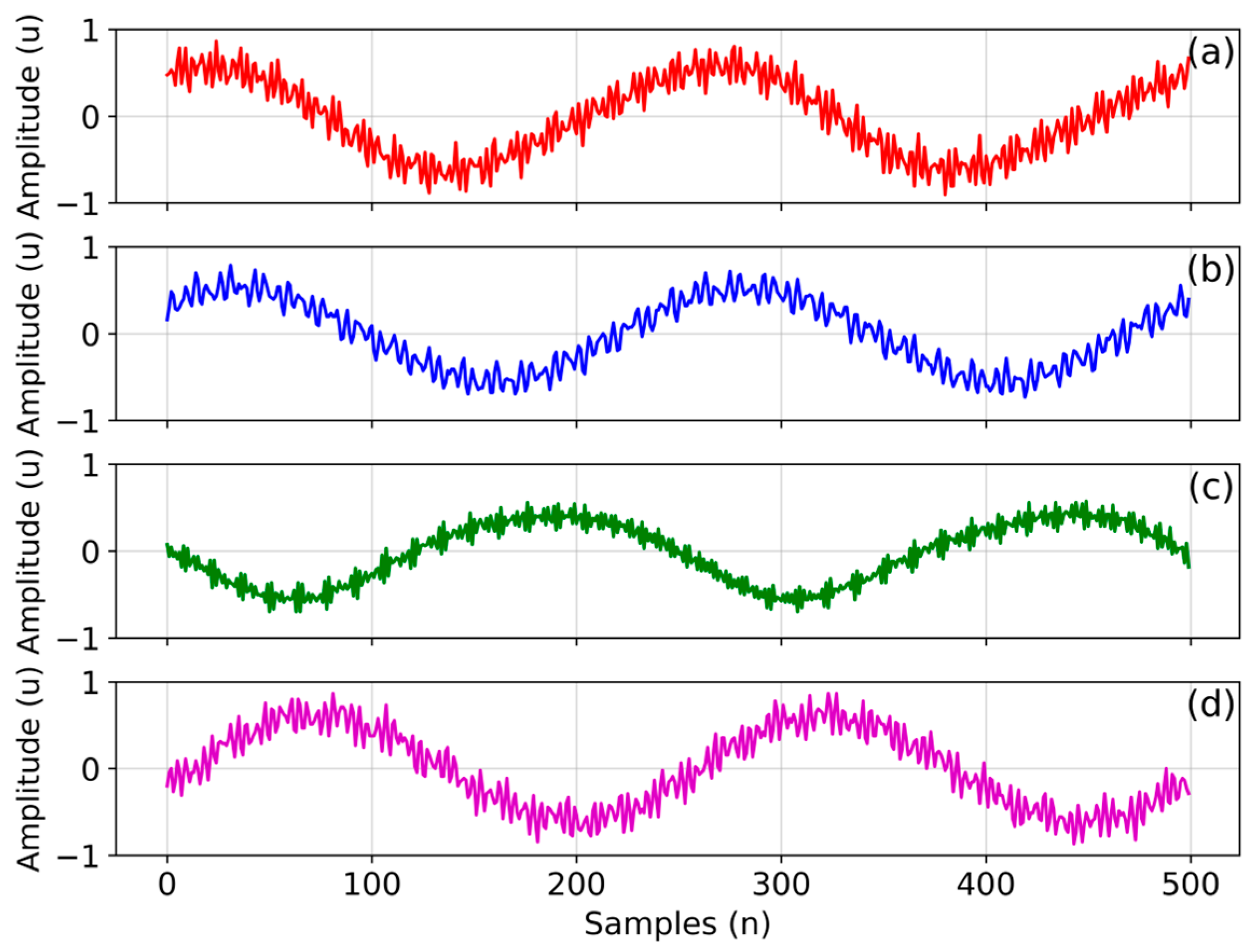
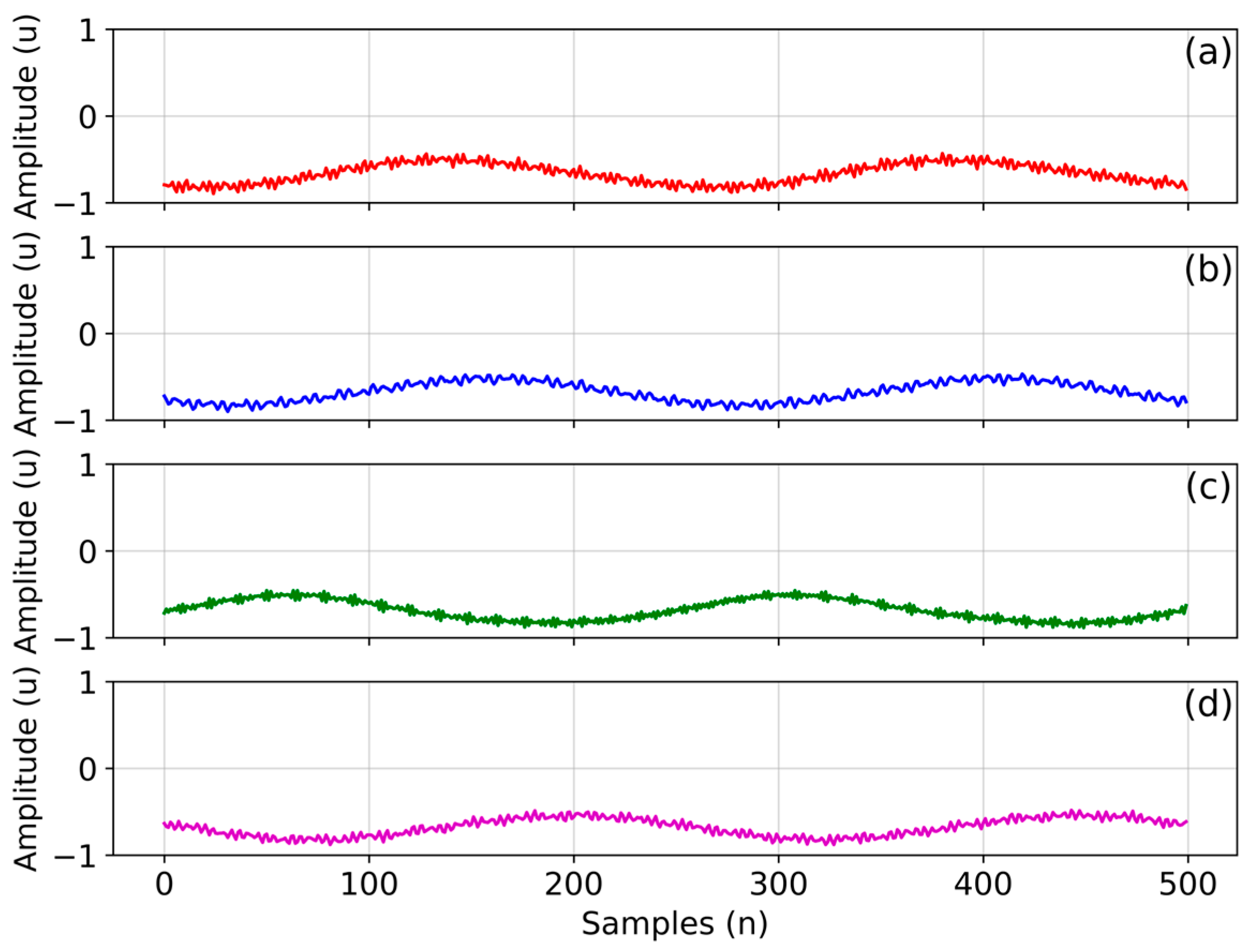
Figure 1 shows the results of one segment of 500 samples of the unprocessed vibration signal acquired from the WTB bolted to P1 for case 1, case 2, case 3, and case 4, corresponding to the WTB healthy, cracked tip, cracked mid, and cracked root, respectively (

Table 2. Case studies of the cracked zones of the WTBs.

Case	Cracked Zones of the WTBs
	Blade’s Position on the Hub
	P1	P2	P3
Case 1	H1	H2	H3
Case 2	CT	H2	H3
Case 3	CM	H2	H3
Case 4	CR	H2	H3
Case 5	H1	CT	H3
Case 6	H1	CM	H3
Case 7	H1	CR	H3
Case 8	H1	H2	CT
Case 9	H1	H2	CM
Case 10	H1	H2	CR

). Relevant information can still be obtained from Figure 1, such as the rotation speed and the accelerations present in the system. However, upon analyzing the signals of each of the acquired cases, it was concluded that it is complicated to classify the cracked WTBs based on the time series results. Thus, directly applying this approach is useless. This complication is due to the rotating nature of the phenomenon and the noise recorded by the sensors.

Figure 2 shows the results of the normalization applied to the vibration signals shown in Figure 1. The normalization provided a better signal definition, making it easier to obtain the rotation frequency based on the signal period. In all the cases, one signal cycle comprises 250 samples, representing a time of 0.25 s or a rotation frequency of 4 Hz. This result matches the value mentioned in the experimental set-up (Section 4.1). Figure 2 illustrates both low and high-frequency content. The low frequency corresponds to the rotation frequency, while the high frequencies are associated with other phenomena; the conditions of the WTB are situated between them. These results demonstrate that although the DAS can easily monitor the WTB, analyzing raw and lightly preprocessed data could detect damage only to transient events. It is due to the minimal or nonexistent differences between the datasets, making it difficult or impossible to recognize characteristic patterns of the different cases analyzed.

3.2. Frequency Domain Analysis

The Discrete Fourier Transform (DFT) was applied to the preprocessed vibration signals. DFT is a frequency domain technique that shows recurrent and periodic time series features. DFT is a commonly used technique for monitoring systems in the industry, specifically on machinery that contains rotating elements. In this case, the spectral analysis was carried out in order to demonstrate that the WTBs are non-identical.

Figure 3 shows the frequency spectra of the preprocessed vibration signals from all the cases mentioned in Table 2. In case 1, where three healthy WTBs are tested, differences are observed in the spectra (Figure 3(a1,b1,c1)). The changes are in frequencies and amplitudes. These differences may be due to slight variations between the blades, which are reflected during the rotational state of the WT. In addition, the natural frequency of the rotating blade in healthy conditions differs from that of the stationary blade, which is 6.64 Hz (Equation (1)). This difference arises because the rotating blade experiences tensile stress from centrifugal force, leading to increased rigidity. This increased stiffness affects the blade’s resonant frequency, leading to more stable rotation.

For cases 2, 5, and 8, where the cracked tip WTB was bolted to P1, P2, and P3, respectively, different spectra patterns are observed for the cracked WTB (Figure 3(a2,b5,c8)). In the aforementioned cases, different spectra patterns are also observed for the healthy WTBs (Figure 3(b2,c2,a5,c5,a8,b8)). For cases 3, 6, and 9, where the middle cracked WTB was bolted to P1, P2, and P3, respectively, many changes in frequencies are observed (Figure 3(a3,b6,c9)). Finally, for cases 4, c 7, and10, where the cracked root WTB was bolted to P1, P2, and P3, respectively, changes are observed between the spectral patterns of healthy WTB (Figure 3(b4,c4,a7,c7,a10,b10)) and between the spectral patterns of cracked WTB (Figure 3(a4,b7,c10)).

The above results confirm that in a classical method for SHM, the crack classes of WTB should be evaluated at the three positions on the hub. At the same time, the healthy WTBs should remain at their initially assigned position during the balancing stage. This last is in order to replicate the real behavior of a small WT. In addition, it can be observed that identifying patterns for the classification of cracked WTBs based on frequency spectra is complex, so an artificial intelligence-based technique facilitates this process. The complexity of the system is due to several causes, including rotational phenomena, the varying locations of cracks, and the effects produced by residual mass imbalance resulting from imperfect manufacturing in WTBs.

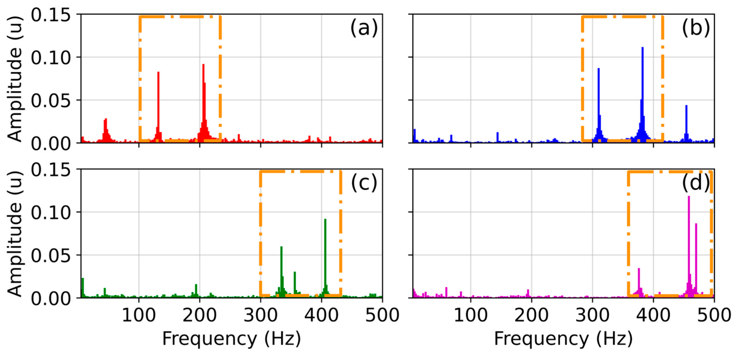
As a result of the analysis of the frequency spectra of diverse experimental tests, it was found that some detected characteristic frequency patterns can be misleading because the spectra show changes and amplitude variations while the test bench remains active over time. Therefore, there are no characteristic frequency patterns between the different samples of their respective case studies. An example of this is shown in Figure 4, corresponding to the frequency spectra obtained from other signal samplings of the WTB bolted to P1 during H, CT, CM, and CR conditions, (a) case 1, (b) case 2, (c) case 3, and (d) case 4, respectively. In a comparison between the spectrums of Figure 3(a1 to a4) and Figure 4, it is seen that the spectrums are significantly different, although they are of the same cases. For this reason, spectral analysis and other conventional techniques cannot be applied to crack identification and location in operating WTB because the techniques require consistent and stable signals, which are not viable for systematic implementation in rotating mechanical elements.

4. Materials and Methods

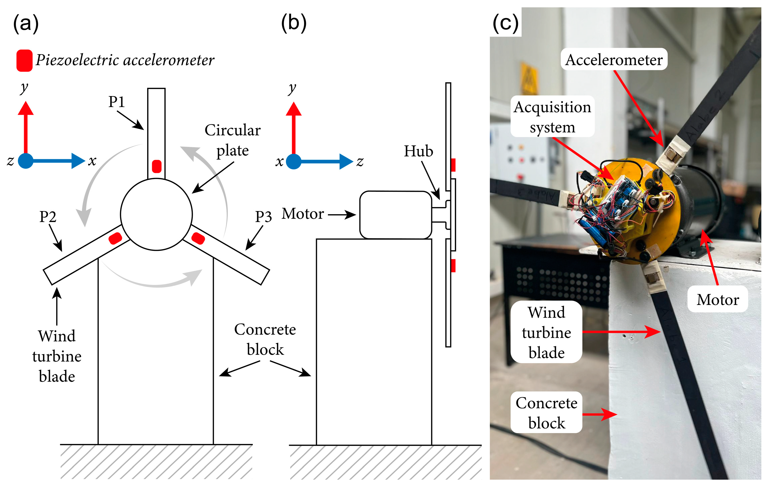
Figure 5 depicts the methodology of this comparative study. The first step of this study involves collecting a dataset of root vibrations from the blades of a three-blade small wind turbine during operation, which fall within the 50 W to 500 W size range of horizontal-axis wind turbines [33]. According to the International Standard IEC 61400-2 [34], small wind turbines are defined as those with a rotor sweep area of less than 200 m² (with a diameter of less than 7.98 m). During the collection of the dataset, some WTBs are healthy with no cracks, while others exhibit cracked zones. The tests were conducted on a test bench in a laboratory under semicontrolled temperature and wind conditions (Figure 6).

The second step of this study involves preprocessing the experimental vibration data, which includes normalization, feature extraction, feature selection, and feature intersection. The third step is training, evaluation, and testing of the different models based on DT, SVM, KNN, and MLP algorithms. The study considered three different sample set sizes $\left(n\right)$ and five different extracted feature sizes $\left(l_m\right)$, leading to the creation and evaluation of a total of 660 distinct ML models. The fourth and fifth steps involve selecting the best models and conducting a comparative analysis of the results obtained.

4.1. Experimental Data Collection

4.1.1. Cracked Zones of the WTBs

For this study, it is first necessary to have a dataset containing the vibration signals generated at the root of each WTB during the WT’s operation, with all three WTBs in a healthy and balanced condition. To build the datasets, the WTBs identified as H1, H2, and H3, with no cracked zone, are bolted to an assigned hub position, identified as P1, P2, and P3 (Figure 6). The configuration assigned is as follows: H1 bolted to P1, H2 bolted to P2, and H3 bolted to P3. After the assignment and assembly of the blades, the balancing process is performed, which involves ensuring that the healthy blades are correctly balanced in their assigned position. After this process, the healthy blades assigned to each position are not replaced or exchanged for another healthy blade, because if so, it is necessary to perform the balancing again. The balancing process is required due to the slight variations in the structural properties of the blades, which, if not considered, generate vibrations that affect the system’s performance.

After the balancing process, it is essential to have a dataset from tests that include two healthy wind turbine blades (WTBs) and one WTB with a cracked zone. To accurately simulate the actual behavior of the small wind turbine during the experimental tests, the two healthy blades must remain the same as those designated for each position during the balancing process. The third blade should be replaced with a blade featuring one of three types of cracked zones: a cracked tip (CT), a cracked middle (CM), or a cracked root (CR) (Table 1).

All case studies or combinations of cracked zones of the three WTBs are shown in Table 2. For instance, in case 2, the WTB bolted to P1 is CT, while the WTB bolted to P2 and the WTB bolted to P3 remain healthy, referred to as H2 and H3, respectively. Alternatively, in case 5, the WTB bolted to P2 is CT, while the WTB bolted to P1 and the WTB bolted to P3 remain healthy, designated as H1 and H3, respectively. In case 8, the WTB bolted to P3 is CT, while the WTB bolted to P1 and the WTB bolted to P2 are healthy, labeled as H1 and H2, respectively.

All the case studies must be considered to identify which of the three WTBs has the crack. Because the WTBs of the same wind generator are not identical, even if they are from the same manufacturer, in practice, the blades of a wind generator have different behavior due to a combination of physical, aerodynamic, and operational factors. The main reasons for this are the wake effect of the WTBs and structural differences between the WTBs.

4.1.2. Experimental Set-Up

For the experimental set-up, parameters and characteristics of a small wind turbine system were considered, such as wind turbine rotation speed, area to place the instrumentation, WTB physical characteristics, and combinations of the cracked zones of the three WTBs. A test bench was designed and built to carry out the experimental tests. The test bench simulates a small wind turbine under operation, so a rotating stimulus was induced on the WTBs. The test bench comprises a concrete block, a 3 HP AC motor, a hub, a holding circular plate, a data acquisition system, three WTBs, and three piezoelectric accelerometers, which are mounted at the root of the WTBs (Figure 6).

The transversal section of each WTB was classified into four zones, as shown in Figure 7. The accelerometers were placed on the root section of each WTB.

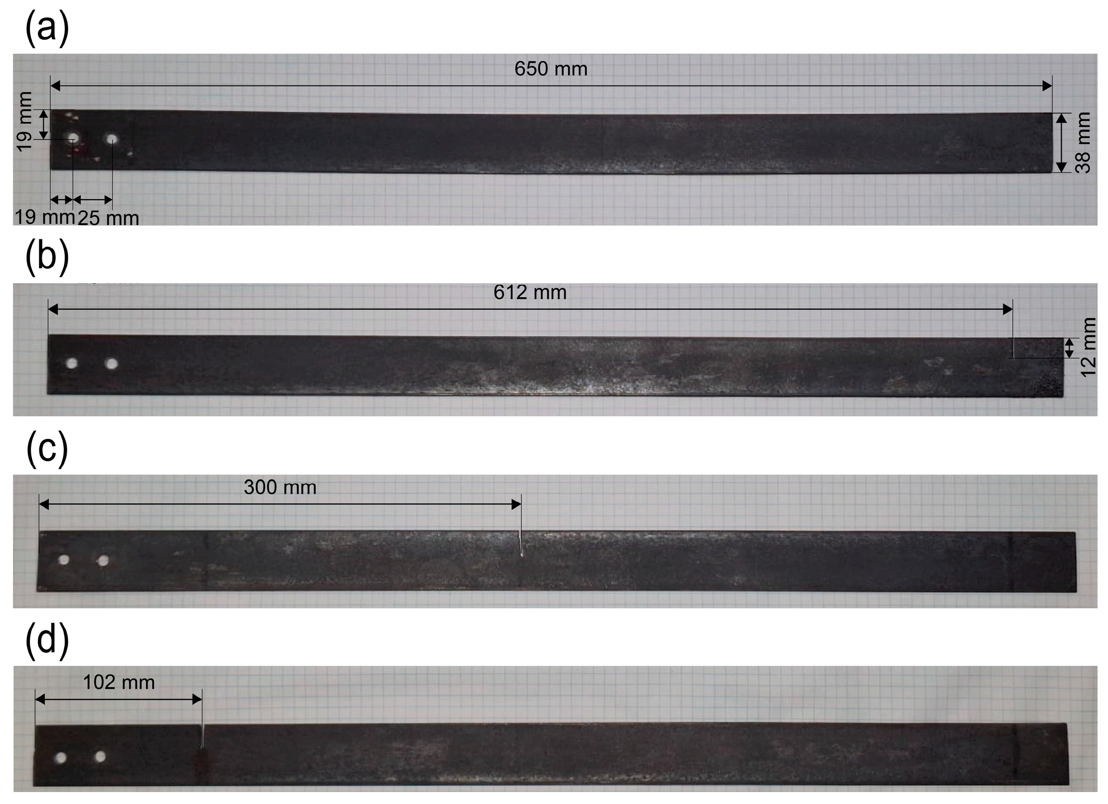
Six WTBs were used for the experimental tests (Table 2), having the following characteristics: semi-uniform profile, ASTM A36, mass of approximately 600 g, homogeneous material, approximately dimensions of 650 mm length, 38 mm width, and 3 mm thick. $\alpha \mathrm{i}\mathrm{s} 1.8775$, $E \mathrm{i}\mathrm{s} 200 \times {10}^9 {\displaystyle \frac{\mathrm{N}}{{\mathrm{m}}^2}}$, $I \mathrm{i}\mathrm{s} \mathrm{8,55} \times {10}^{-11} {\mathrm{m}}^4, A \mathrm{i}\mathrm{s} 1.14 \times {10}^{-4} {\mathrm{m}}^2, \mathrm{a}\mathrm{n}\mathrm{d} \rho \mathrm{i}\mathrm{s} 7850 {\displaystyle \frac{\mathrm{k}\mathrm{g}}{{\mathrm{m}}^3}}$ (Figure 4). The fixation points of the WTB were made through 6 mm drill holes. The distance between holes is 25 mm, and the distance from the border of the WTB is 19 mm. Both drill holes are aligned with the center of the profile. The cracks were emulated through incisions 1 mm thick and 12 mm deep. The cracked zones of the WTBs were performed at different distances from the fixation zone, as shown in Figure 8. Currently, there are no established standards or regulations that specify the dimensions or criteria for manually induced cracks in WTBs. In this study, as well as in other research focused on monitoring blade cracks, the size of the induced cracks was intentionally chosen to realistically simulate actual damage by making cross-cuts in the blade laminate.

In this study, the $S_R$ of the blade was 240 rpm, which is an $f_R$ of about 4 Hz (Equation (3)), an $f_{BP}$ of 12 Hz (Equation (4)), an $a_c$ of 473.75 m/s² (Equation (5)) (approximately 48 g), and an $a_t$ of 0 m/s² (Equation (6)) due to the constant rotation speed, while the minimum resonant frequency of a stationary blade is 6.64 Hz (Equation (1)).

The flap-wise vibration was acquired for the three WTBs. This direction was selected because of the system’s behavior, as it experiences centripetal accelerations in the WTBs. The tests demonstrated the above, as the edge-wise vibration is perceptible but unstable for data acquisition, making it unreliable.

4.1.3. Data Acquisition System

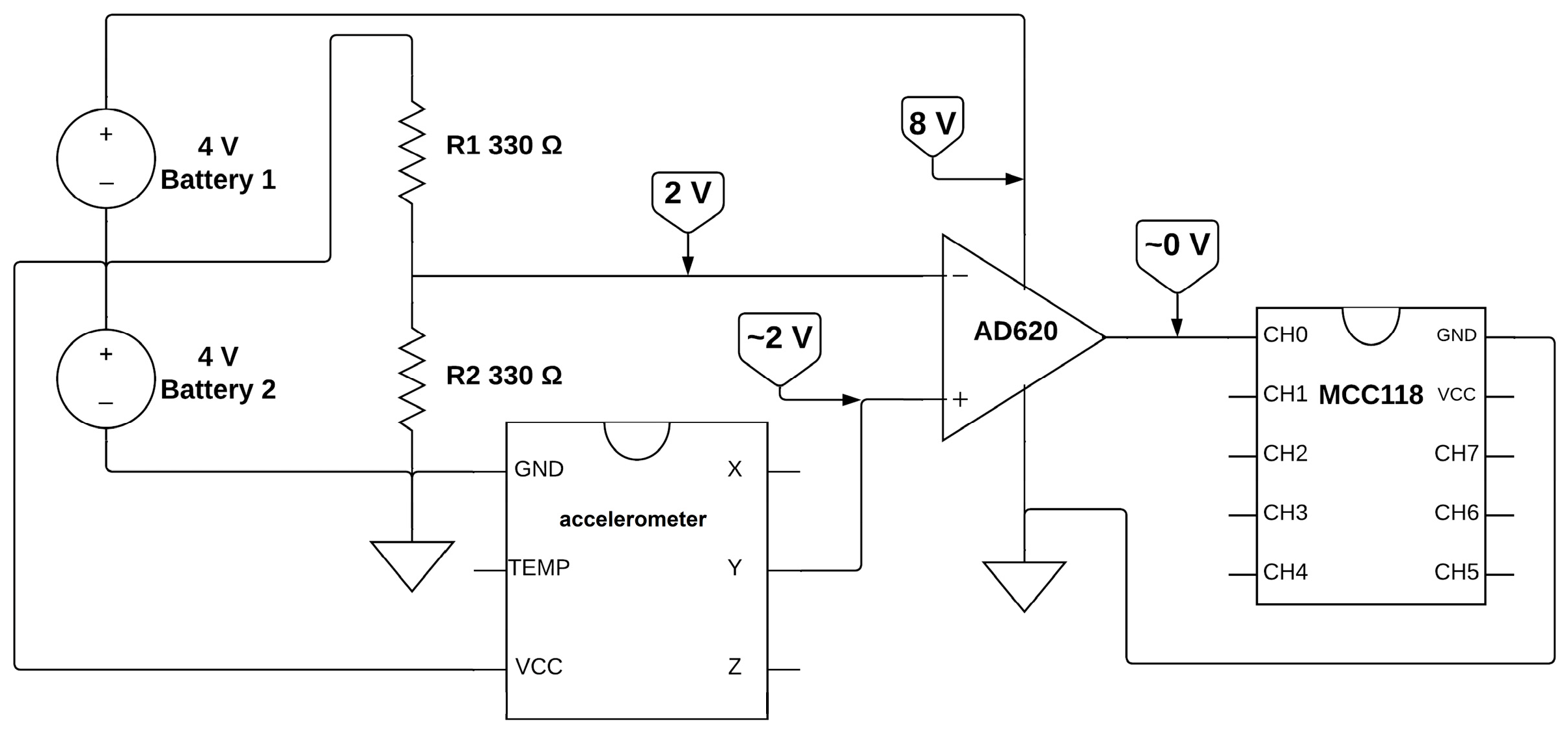
The data acquisition system (DAS) comprises three piezoelectric accelerometers, a signal conditioner module AD620, a Raspberry Pi model 4B+ 8 GB (The Raspberry Pi Foundation, Cambridge, UK), batteries of 2200 mAh, a power bank of 10,000 mAh, and a voltage measurement DAQ HAT for Raspberry Pi model MCC 118 (Digilent co NI, Austin, TX, USA) (Figure 6 (c)). The MCC 118 allows a max sampling rate of 100,000 Hz on a single-channel set-up and 8 MCC 118 boards to be stacked to expand the number of channels available. The programming language used was Python (version 3.12.1). The sensors were selected based on their capabilities to cover the magnitude and bandwidth of the phenomena (Equations (3) to (6)). In this implementation, the accelerometers selected are piezoelectric because the system is a rotating element. The accelerometers selected can register up to ±500 g and have a 2 Hz to 10,000 Hz bandwidth. The accelerometers were connected to the signal conditioner to remove the DC component from the sensors and then to amplify the signal. The batteries were connected to a voltage divider circuit to obtain three different voltages, as shown in Figure 9.

Three three-dimensional datasets, denoted as $C_e\in {\mathbb{R}}^{r\times n\times p}$, were acquired, with the parameters $r$ equal to 7680, $p$ equal to 3, $n\in \left\{\mathrm{500,1000,5000}\right\}$, and $e$ ranging from 1 to 3. The data were sampled at a $f_s$ of 1 kHz. Each element $c_{ijk}\in \mathbb{R}$ represents the feature $k$ of the sample $j$ in replicate $i$. Each dataset $C_e$ contains balanced subdatasets of samples from the ten case studies listed in Table 2.

4.2. Preprocessing of Vibration Datasets and Development of ML Models

4.2.1. Preprocessing of Vibration Datasets

Effective preprocessing is essential for building a successful artificial intelligence model. Proper data preparation improves the model’s performance and ensures the data is formatted suitably for training.

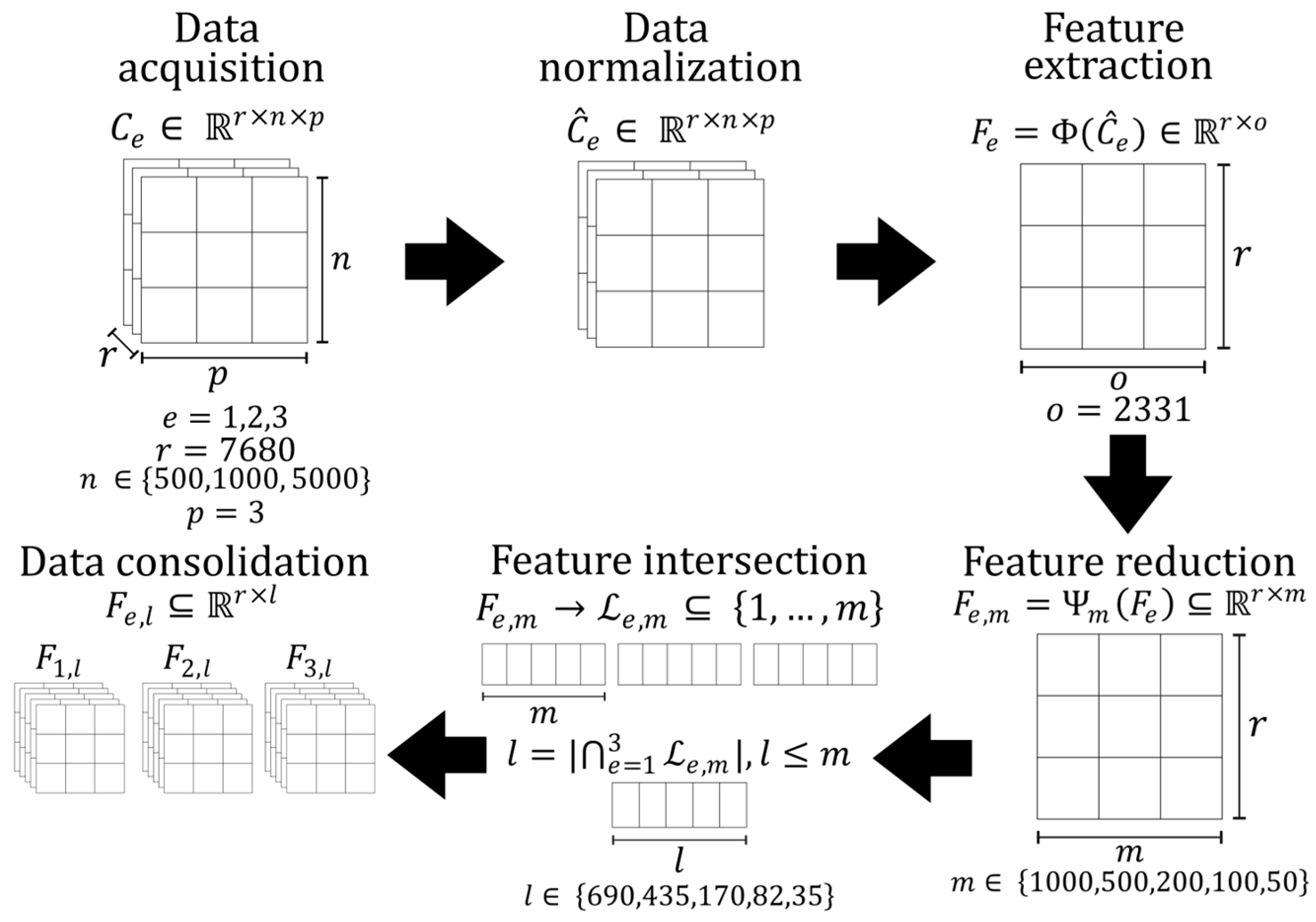
The programming language used was Python 3.12.1. The methodology for pre-processing vibration datasets consists of several stages (Figure 10), detailed in the following steps:

• Import the Scikit-learn (version 1.4.1) library and TSFresh (version 0.20.2) library.
• Load and normalize the three datasets $C_e$. The normalization is performed by absolute maxima per characteristic, obtaining ${\widehat{C}}_e\subseteq {\left[-\mathrm{1,1}\right]}^{r\times n\times p}$, where each element was transformed as ${\widehat{c}}_{ijk}={\displaystyle \frac{c_{ijk}}{\underset{i,j}{\mathit{max}}\left|c_{ijk}\right|}}$ for each $k\in \left\{\mathrm{1,2},3\right\}$. The function normalize() was used for this process.
• Extract the features of the normalized datasets ${\widehat{c}}_{ijk}$. Extraction is carried out by a transformation $\mathsf{\Phi }:{\mathbb{R}}^{r\times n\times p}\to {\mathbb{R}}^{r\times o}$, where $o$ is 2331. To accomplish this, the TSFresh (version 0.20.2) library is used, which calculates diverse features from time series data, generating the datasets $F_e=\mathsf{\Phi }\left({\widehat{C}}_e\right)\in {\mathbb{R}}^{r\times o}$. The features encompass various domains, including statistical, temporal, and spectral properties. In this study, the features with high computational costs were not calculated. To do that with TSFresh 0.20.2, a custom settings object was used for the feature extractors: EfficientFCParameters(). This was used because the runtime performance plays a major role.
• Select the extracted features using a function $\mathsf{\Psi }:{\mathbb{R}}^{r\times o}⟶{\mathbb{R}}^{r\times m}$, implemented with the Scikit-learn() library, obtaining the data subsets $F_{e,m}={\Psi }_m\left(F_e\right)\subseteq {\mathbb{R}}^{r\times m}$ with $m\in \left\{\mathrm{50,100,200,500,1000}\right\}$
• Define the set of indices of extracted features ${\mathcal{L}}_{e,m}\subseteq \left\{1,\dots ,m\right\}$; this is done for each dataset $F_{e,m}$. For this purpose, standard feature indices are identified by the intersection at the index level, defined as $l=\left|\bigcap _{e=1}^3{\mathcal{L}}_{e,m}\right|,l\le m$. The common indexes found for each value of $m$ were denoted as ${\mathcal{l}}_m\in \left\{35,82,170,435,690\right\}$
• Define the reduced datasets $F_{e,l}\subseteq {\mathbb{R}}^{r\times l}$ that will be used to create the ML models.

Figure 10. Stages of the preprocessing of vibration data.

Figure 10. Stages of the preprocessing of vibration data.

The TSFresh library incorporates 93 calculator functions with which the features presented in this study are generated. The calculator’s functions and features can be categorized into five groups to simplify their analysis, which include Descriptive, Dependency, Complexity, Frequency, and Events.

The calculator functions as well as the Descriptive type features correspond to values derived directly from the analysis of time series, such as the mean, median, maximum, and minimum; these are useful for rapid exploratory and comparative analyses between datasets. The functions and features of the Dependency type serve to identify the correlation between the points in the time series and its internal structure. They allow for the identification of patterns of periodicity and seasonality, as well as the relationship of previous data with future data. Examples of this are self-correction and linear trend. The functions and features of the Complexity type make it possible to assess the level of irregularity of the time series, allowing for the differentiation of time series with a predominance of noise from structured time series. The most prominent example is entropy. The functions and features of the Frequency type are based on the transformation of the time series to the frequency domain, so the information is presented in the form of spectra. These features can detect characteristic marks of the signal that are not visible in the time domain, so they are used in industrial, medical, and other environments. Examples of such features are the Fourier transform and the Wavelet transform.

In the context of detecting cracks in WTBs, the distribution of feature types directly reflects how the analysis of vibration signals evolves from simple summaries to more sophisticated indicators of damage. At early stages, Descriptive features (such as mean or variance) can help establish baseline behaviors of a healthy blade. However, they are not sufficient to capture subtle patterns caused by cracks. As the number of extracted features grows, Dependence features become dominant, which is highly relevant because cracks often alter the temporal correlations and dynamic relationships within vibration signals. Similarly, the increase in Frequency features is crucial, since blade cracks typically introduce changes in spectral components, such as harmonics or sidebands, that are best identified in the frequency domain. Event-based features also gain importance in larger feature sets, as they can highlight transient behaviors or sudden impacts associated with crack propagation. Although Complexity features remain less dominant, their ability to capture irregularities and non-linear behaviors adds complementary insight. Thus, the progression from descriptive to dependence, frequency, and event-based features mirrors the transition from general monitoring to more precise and sensitive detection methods, making it possible to identify early-stage cracks in wind turbine blades before they lead to critical failures.

4.2.2. Development and Assessment of ML Models

In this comparative study, four typical machine learning algorithms were selected for crack detection, identification of cracked blades, and localization of crack areas in small wind turbine blades under operational conditions. The selection of these algorithms was based on the most frequently studied in the literature for wind turbine failure detection. The algorithms selected were DT [13,14], SVM [1,5], KNN [35,36], and MLP [1]. These algorithms have been widely applied, as they are characterized by being easily replicable in limited systems and therefore do not require sophisticated computing equipment. Additionally, these algorithms perform well with limited datasets, without sacrificing performance, making them ideal for on-site deployment. In contrast to more robust or complex models, which can produce higher precision and accuracy margins at the expense of interpretability, the selected algorithms are easily interpretable, allowing for direct auditing of critical systems using the characteristics analyzed. The selected algorithms are easily operable, exhibiting both low and high complexity characteristics, as well as large numbers, with relatively small sample sizes.

The selected algorithms were applied to the preprocessed datasets $\left(F_{e,l}\right)$, leading to the creation and evaluation of different ML models. Functions such as ${\mathcal{A}}_{u,v}:{\mathbb{R}}^{r\times l}\times {\mathbb{R}}^r⟶\mathcal{H}$ were defined to create the different ML models. Here, $u\in \left\{\mathrm{1,2},\mathrm{3,4}\right\}$represents the algorithm, and $v\in \left\{1,\dots ,V_u\right\}$ represents one of its variants. The resulting ML models were denoted as $h_{e,l}^{(u,v)}={\mathcal{A}}_{u,v}(F_{e,l},y)\in \mathcal{H}$.

The programming language used was Python (version 3.12.1). A laptop equipped with an Intel Core i7-11800H processor, an NVIDIA GeForce RTX 3070 Laptop GPU, and 32 GB of DDR4 RAM was used for implementing the models. The methodology used in the training, validation, and testing stages of the different ML models consists of the following steps:

• Import the Pandas (version 2.2.0), NumPy (version 1.26.4), Matplotlib (version 3.8.2), and Scikit-learn (version 1.4.1) libraries. From the latter library, select the respective modules to evaluate the algorithms: DT, SVM, KNN, and MLP.
• Load the preprocessed datasets $F_{e,l}$ and the target vector $T_e$, and then divide them into data subsets. The percentages of data selected for training, validation, and testing were 60%, 20% and 20%, respectively. The train_test_split() function was used to partition datasets in a balanced and random manner.
• Identify and select the hyperparameters for each of the four selected algorithms, resulting in 660 distinct ML models ${(h}_{e,l}^{(u,v)})$. The distribution of these ML models was as follows: 180 for DT, 180 for SVM, 120 for KNN, and 180 for MLP. The selected and configured hyperparameters for each algorithm are described below:

• Decision Trees Algorithm

In the DT algorithm, two hyperparameters were selected for variation: the maximum depth of the tree and the minimum number of samples required to perform a split. The maximum depth of the tree was set to four levels: 3, 5, 10, and no limit. Additionally, the minimum number of samples needed to split a node was configured to be 2, 5, and 10 samples. These combinations of hyperparameters resulted in a total of 12 different configurations.

• Support Vector Machine Algorithm

In the SVM algorithm, three hyperparameters were chosen for variation: the penalty parameter C, the gamma coefficient, and the kernel type. The parameter C was evaluated with values of 0.1, 1, and 10. The gamma hyperparameter was tested using the options scale and auto. Lastly, the kernel type was set to either rbf or linear. In total, 12 different configurations were evaluated for this algorithm.

• KNN Algorithm

In this analysis of the KNN algorithm, two hyperparameters were varied: the number of neighbors and the type of weighting. The number of neighbors was set to 3, 5, 10, and 15. The weighting was tested using both uniform and distance schemes. As a result, a total of 8 different configurations were generated for the algorithm.

• MLP Algorithm

For the MLP model, five main hyperparameters were selected: the size of the hidden layers, the number of neurons, the activation function, the regularization parameter (α), and the maximum number of iterations. The model utilized one hidden layer, and the number of neurons was varied at 100, 300, and 500. The activation functions evaluated were the rectified linear unit (ReLU) and the hyperbolic tangent function (tanh). The regularization parameter (α) was set to values of 0.0001 and 0.001. The maximum number of iterations was limited to 500. In total, 12 different configurations were assessed for this algorithm.

4.

Train and adjust the ML models $\left(h_{e,l}^{(u,v)}\right)$ using the training data subset, which comprises elements from $F_{e,l}$and $T_e$. The GridSearchCV() function was used to configure hyperparameters. This function enables the automatic adjustment and optimization of hyperparameters by exhaustively searching for predefined combinations. The GridSearchCV() function is based on k-fold cross-validation, which is ideal for small datasets or when robust evaluation is required. Thus, GridSearch() completely automates the selection of the best model by a reliable statistical procedure. The metrics computed were the F1-score, fit time, and test-time training.

5.

Validate the 660 ML models using the validation dataset subset, which comprises elements from $F_{e,l}$. The metrics calculated are F1-score, Accuracy, Precision, and Recall. The validation is not strictly necessary when applying k-fold cross-validation; however, it is performed given the availability of data. This validation ensures a robust evaluation and avoids over-adjustments and bias in model selection. The factors considered to reduce bias are: use of balanced datasets, inclusion of a sufficient number of samples with relevant characteristics for the models being analyzed, evaluation of various dataset sizes, implementation of double validation, including K-Folds cross-validation during training and external validation during testing.

6.

Test the 660 ML models using the test data subset, which comprises elements from $F_{e,l}$. The metrics calculated are F1-score, Accuracy, Precision, and Recall.

7.

Plot the multiclass confusion matrix of the 660 ML models. These matrices are obtained using sklearn metrics and matplotlib.pyplot module.

8.

Calculate the F1-score metrics in three modes: macro, micro, and weighted. The F1-score (macro) evaluates the model using perfectly balanced data. The F1-score (micro) is applied when the data is unbalanced, taking into account the number of samples for each case. Lastly, the F1-score (weighted) evaluates the model based on the frequency of occurrence of each case.

After completing the training, validation, and testing of the 660 ML models, the ML models with the best metrics and performance times were selected in each of the three datasets, which have dimensions of 500, 1000, and 5000 samples, corresponding to experiment times of 0.5 s, 1 s, and 5 s. This selection includes the 20 ML models with the highest mean test scores and the shortest total time, resulting in a collection of 60 machine learning models. From these models, a comparative analysis was conducted of those that achieved test scores exceeding 90%, 95%, and 98%. Additionally, a comparative analysis of the models with the longest and shortest training times was conducted.

On the other hand, an analysis is conducted on the metric values and performance times obtained from the validation and test steps applied to the best model of each machine learning algorithm.

5. Results and Discussions

5.1. Feature Extraction

Table 3. Distribution of the extracted and selected features.

Type of Features	Distribution (%)
	Features Size
	35	82	170	435	690
Descriptive	94.29	48.78	30.00	14.02	10.29
Dependence	2.86	39.02	51.76	51.03	40.43
Complexity	2.86	4.88	7.06	12.41	9.42
Frequency	0.00	1.22	1.76	8.28	24.93
Events	0.00	6.10	9.41	14.25	14.93

shows the analysis of the distribution percentage by feature type of the extracted and selected features.

The distribution of features shows a clear evolution as the total number of extracted features increases. With small feature sets, Descriptive statistics dominate, representing over 90% of the total when only 35 features are considered. However, as the number of features grows, their relative importance decreases significantly, giving way to more advanced categories. Dependence features quickly rise to become the most representative group, stabilizing around 40–50% in larger sets, which highlights their central role in capturing temporal and relational patterns within the data. At the same time, Frequency and Event-based features, which are absent in small sets, gain substantial weight as the feature pool expands, reaching nearly 25% and 15%, respectively, at 690 features. Complexity features, although increasing modestly, remain secondary compared to the other categories. Overall, the trend indicates a shift from simple descriptive measures to a more balanced and diverse feature set, where dependence, frequency, and event-based features play a dominant role in richer extractions.

The analysis reveals that as the number of extracted features increases, the representation shifts from simple Descriptive measures toward a more diverse and balanced set, where Dependence, Frequency, and Event-based features gain prominence, enhancing the capability to capture complex patterns and behaviors in the data.

5.2. Training and Fitting the Best Machine Learning Models

Figure 11 presents the results of the metrics calculated during the training and tuning of the 60 best-performing machine learning models, selected based on the highest mean test scores and the lowest total time. Each model is identified by its number and the base algorithm it uses. The graphs are organized according to three dataset sizes $(n\in \left\{500,1000,5000\right\})$ and the dimensions of the extracted features ${(\mathcal{l}}_m\in \left\{\mathrm{35,82,170,435,690}\right\})$. Specifically, Figure 11a displays the metrics results for the 20 datasets containing 500 samples, representing an experimental test duration of 0.5 s. Figure 11b illustrates the metrics results for the 20 datasets with 1000 samples, corresponding to a 1 s experimental test. Meanwhile, Figure 11c shows the metric results for the 20 datasets, which consist of 5000 samples and have a duration of 5 s of experimental testing.

By selecting models with a mean test score greater than 90% during the training and fitting stage, 45 machine learning models were obtained. The distribution of these models based on the algorithms used is as follows: 33.33% are DT, 28.89% are SVM, 20.00% are KNN, and 17.78% are MLP. The distribution of the 45 machine learning models based on the number of features extracted ${(\mathcal{l}}_m)$ is as follows: 22.22% for ${\mathcal{l}}_m$ = 35, 24.44% for ${\mathcal{l}}_m$ = 82, 26.67% for ${\mathcal{l}}_m$ =170, 13.33% for ${\mathcal{l}}_m$ = 435, and 13.33% for ${\mathcal{l}}_m$ = 690. While the distribution of the 45 machine learning models according to experiment time or sample number $\left(n\right)$, remains balanced with 33.33% for $n\in \left\{\mathrm{500,1000,5000}\right\}$. This initial filtering of machine learning models indicates that the nature of the data favors both DT and SVM models, as well as datasets with a reasonable number of extracted features $\left({\mathcal{l}}_m\right)$. However, the experiment time or number of samples does not appear to affect the mean test score of the machine learning models.

As a result of selecting models with a mean test score greater than 95% during the training and fitting stage, 37 machine learning models were obtained. The distribution of these models by algorithm is as follows: 32.43% for DT, 29.73% for SVM, 21.62% for KNN, and 16.22% for MLP. Whereas, the distribution of the 37 machine learning models based on the number of features extracted ${(\mathcal{l}}_m)$ is as follows: 10.81% for ${\mathcal{l}}_m$ = 35, 27.03% for ${\mathcal{l}}_m=$ 82, 32.43% for ${\mathcal{l}}_m=$ 170, 13.51% for ${\mathcal{l}}_m$ = 435, and 16.22% for ${\mathcal{l}}_m=$ 690. Finally, when analyzing the distribution of the models according to experiment time or sample size $\left(n\right)$, the results were as follows: 32.43% for $n$ = 500, 32.43% for $n$ = 1000, and 35.14% for $n$ = 5000. This second round of filtering confirms that the nature of the datasets favors DT and SVM models. In comparison to the 45 machine learning models that had a mean test score between 90% and 95%, the 37 models with scores above 95% show that datasets with 82 and 170 extracted features achieve the highest performance, appearing in about two-thirds of the selected models. Notably, no significant effect is observed regarding the performance of the models based on sampling time or the number of samples.

For a mean test score value greater than 98% during the training and fitting stage, the selection of machine learning models was drastically reduced to 13. The distribution of these models based on the algorithms used is as follows: 46.15% for DT, 7.69% for SVM, 23.08% for KNN, and 23.08% for MLP. When categorized by the number of features extracted ${(\mathcal{l}}_m)$, the distribution is: 0% for ${\mathcal{l}}_m$ = 35, 23.08% for ${\mathcal{l}}_m$ = 82, 53.85% for ${\mathcal{l}}_m$ = 170, 7.69% for ${\mathcal{l}}_m$ = 435, and 15.38% for ${\mathcal{l}}_m$ = 690. In terms of experiment time or sample size ($n)$, the distribution is as follows: 23.08% for $n$ = 500, 30.77% for $n$ = 1000, and 46.15% for $n$ = 5000. This analysis confirms that the nature of the data predominantly supports the use of DT models. However, SVM models lag significantly behind both KNN and MLP models. Notably, the sets with 170 extracted features account for more than half of the selected models. Lastly, we observed that sampling time, or the number of samples, significantly impacts model performance, with sets containing $n$ = 5000 representing twice the percentage of models compared to those with $n$ = 500.

The following analysis presents the minimum and maximum execution times of machine learning models that achieved a mean test score greater than 90% during the training and fitting stages. The results are organized by algorithm type. For the DT-based models, the recorded run times ranged from 0.083665 s to 2.102346 s. The SVM models exhibited a wider range, with execution times from 0.548840 s to 259.081404 s. The KNN models had run times ranging from 0.092199 s to 0.349957 s. In contrast, the MLP models had the longest execution times, ranging from 12.374451 s to 34.133011 s.

For models that achieved a mean test score exceeding 95%, the minimum and maximum execution times remained consistent with the previously reported values, except for the minimum time for the DT-based models, which was noted as 0.242134 s. Additionally, in models that reached a mean test score greater than 98%, changes were observed in the maximum execution times for DT and MLP-based models, recorded at 1.933996 s and 28.310107 s, respectively. A variation in the minimum run time for KNN models was also noted, with a value of 0.189169 s. In the case of the DT-based model, both the minimum and maximum run times were recorded as 27.854260 s, as only one model of this type was evaluated below that performance threshold. This level of filtering helps identify models with lower computational costs while still maintaining effective classifier performance. Overall, algorithms like KNN and DT demonstrate considerably shorter execution times compared to SVM and MLP, whose times can be hundreds of times longer.

Table 4. Configured hyperparameters of the 13 ML models with a mean test score higher than 98%.

ML Model ID	Hyperparameters
M290-KNN	{‘n_neighbors’: 3, ‘weights’: ‘distance’}
M334-KNN	{‘n_neighbors’: 3, ‘weights’: ‘distance’}
M384-KNN	{‘n_neighbors’: 15, ‘weights’: ‘distance’}
M186-DT	{‘max_depth’: None, ‘min_samples_split’: 2}
M582-DT	{‘max_depth’: None, ‘min_samples_split’: 2}
M230-DT	{‘max_depth’: None, ‘min_samples_split’: 2}
M362-DT	{‘max_depth’: None, ‘min_samples_split’: 2}
M494-DT	{‘max_depth’: None, ‘min_samples_split’: 2}
M626-DT	{‘max_depth’: None, ‘min_samples_split’: 2}
M172-MLP	{‘activation’: ‘tanh’, ‘alpha’: 0.0001, ‘hidden_layer_sizes’: (300,), ‘max_iter’: 500}
M308-MLP	{‘activation’: ‘tanh’, ‘alpha’: 0.001, ‘hidden_layer_sizes’: (500,), ‘max_iter’: 500}
M352-MLP	{‘activation’: ‘tanh’, ‘alpha’: 0.001, ‘hidden_layer_sizes’: (500,), ‘max_iter’: 500}
M376-SVM	{‘C’: 10, ‘gamma’: ‘auto’, ‘kernel’: ‘linear’}

displays the model number, base algorithm, and configured hyperparameters for each of the 13 machine learning models that achieved a mean test score exceeding 98% during the training and fitting stages.

Table 5. Execution conditions and metric results of the 13 selected ML models.

ML Model ID	Samples Size	Number of Extracted Features	Mean Test Score (%)	Fit Time (s)	Test-Time Training (s)
M290-KNN	500	170	99.457924	0.016667	0.333290
M334-KNN	1000	170	99.763227	0.013929	0.314670
M384-KNN	5000	170	99.956203	0.012772	0.176397
M186-DT	1000	82	98.048445	0.251715	0.005092
M582-DT	1000	690	98.131035	1.927447	0.006549
M230-DT	5000	82	98.631999	0.237539	0.004596
M362-DT	5000	170	98.670310	0.440474	0.004000
M494-DT	5000	435	98.917577	1.053872	0.005671
M626-DT	5000	690	98.939005	1.818627	0.010165
M172-MLP	500	82	98.065060	28.286602	0.023505
M308-MLP	500	170	99.001571	15.017870	0.011996
M352-MLP	1000	170	99.175577	12.361673	0.012777
M376-SVM	5000	170	98.607833	27.831921	0.022339

provides details on the number of samples $\left(n\right)$, the number of extracted features $\left(l_m\right)$, the mean test score, the test-time training, and the fit time for the 13 machine learning models selected for their optimal performance during the training and fit stages.

A performance overview of the 13 machine learning models is presented below. The KNN models achieved the highest overall accuracy, ranging from 99.46% to 99.96%. The best-performing model, identified as M384-KNN, achieved an accuracy of 99.96%, demonstrating both high performance and consistency across the models. These results establish KNN as the most effective algorithm in terms of predictive accuracy among the four models evaluated. The MLP models also performed well, with accuracies ranging from 98.07% to 99.18%. The top MLP model, M352-MLP, achieved an accuracy of 99.18%, making MLP the second most accurate overall. However, the wider accuracy range observed in MLP models suggests some variability depending on model configuration or training conditions.

In contrast, the DT models had a lower accuracy range of 98.05% to 98.94%, with the model identified as M626-DT achieving the highest accuracy. Although DT models are quick to train and test, their predictive performance is lower compared to both KNN and MLP models, which may limit their suitability for tasks requiring high accuracy. Finally, only one model from the SVM category was recorded, achieving an accuracy of 98.61%. This result places the SVM model slightly above average DT performance but below the top-performing models from both KNN and MLP. With just one data point, it is not easy to assess the consistency or variability of SVM performance. In summary, the KNN models stand out as the top performers in terms of accuracy, while the MLP models offer a strong alternative with slightly lower but still competitive accuracy. Meanwhile, SVM and DT models lag, making them less favorable for tasks where maximum predictive performance is critical.

The following is a comparative analysis of the fitting times for 13 top-performing machine learning models. Among these, the KNN models stand out for their efficiency, with fitting times ranging from approximately 0.013 s to 0.017 s. The fastest model, identified as M384-KNN, takes 0.0128 s, while the slowest model, M290-KNN, takes 0.0167 s. This narrow range suggests consistent performance across the KNN models. In contrast, the DT models exhibit moderate fitting times, which range from 0.24 s to 1.93 s. Though slower than the KNN models, the DT models still train relatively quickly compared to more complex alternatives. The fastest DT model, M230-DT, fits in 0.2375 s, whereas the slowest, M582-DT, takes 1.9274 s. This nearly eight-fold increase indicates variability in the complexity or data handling capabilities of the DT models. The MLP models have significantly higher fitting times, ranging from 12.36 s to 28.29 s. The slowest model, M172-MLP, is more than twice as slow as the fastest model, M352-MLP. This substantial variance is likely attributable to factors such as network depth and hyperparameter settings, making the MLP models more computationally expensive to train than both the KNN and the DT models. Finally, the SVM model, which has only one recorded instance (M376-SVM), has a fitting time of 27.83 s. Although there is no range for the SVM, this fitting time places it among the slowest models, comparable to the slower MLP models. Hence, like the MLP models, the SVM model is not ideal for scenarios requiring rapid training. Overall, the KNN models are the clear winners in terms of training efficiency. In contrast, the MLP models and the SVMs offer complex modeling capabilities at the expense of longer fitting times.

On the other hand, the DT algorithm demonstrates the fastest overall performance during testing, with a training time ranging from approximately 0.0046 s to 0.0066 s. The quickest model, identified as M230-DT, completed testing in 0.0046 s, whereas the slowest model, M582-DT, took 0.0065 s. In contrast, the MLP exhibits a broader range of testing times, from about 0.012 s to 0.23 s, indicating more variability among its models. The fastest MLP model, M308-MLP, achieved a time of 0.0119 s, while the slowest, M172-MLP, took significantly longer at 0.2300 s. The support vector machine (SVM) shows a consistent test-time performance of 0.0223 s, represented solely by model M376-SVM, with no slower counterpart available. The KNN algorithm displayed the broadest range of testing times, from approximately 0.176 s to 0.333 s. The fastest KNN model, M384-KNN, completed testing in 0.1763 s, while M290-KNN was the slowest at 0.3333 s.

In summary, DT is the most efficient algorithm in terms of test speed, followed by SVM, MLP, and KNN. KNN has the slowest performance and the most significant variability. Although MLP can sometimes be faster than SVM, its high variability makes it less consistent in performance compared to SVM.

The comparative analysis of scalability and the impact of sample size reveals the following insights: The KNN algorithm shows improved accuracy with an increased sample size while maintaining low training times. However, it suffers from high prediction times due to its instance-based nature. The DT models experience slight benefits from an increased dataset and remain efficient in both training and prediction processes. The MLP demonstrates improved accuracy with more features but faces high training times, particularly when dealing with larger datasets. The SVM, tested with a single instance comprising 5000 samples and 170 features, exhibits decent performance but incurs a high training cost.

The comparative analysis of feature count impact is presented here. The high-performing models, particularly KNN and SVM, consistently utilized 170 features, indicating an optimal balance between input complexity and performance for these algorithms. While the DT models with fewer features—such as 82 or 435—still performed reasonably well, the highest accuracy for DTs was achieved using 690 features, as demonstrated by models like M582-DT and M626-DT. This finding suggests that while DTs can operate effectively with a limited number of features, increasing the richness of the feature set can further enhance their performance. More complex models, such as MLP and SVM, significantly benefit from richer feature sets, allowing them to capture more intricate patterns. However, this also results in increased training time. Overall, having a richer set of features generally improves model accuracy, especially for more sophisticated algorithms like MLP and SVM.

5.3. Validation and Testing of the Best Machine Learning Models

Table 6. Results of metrics calculated during the validation of the best machine learning models for each algorithm used.

ML Model ID	Metrics
	F1-Score (%)	Accuracy (%)	Precision (%)	Recall (%)
M334-KNN	99.511134	99.544271	99.510318	99.513605
M186-DT	98.538972	98.632813	98.562813	98.541709
M352-MLP	98.185053	98.242188	98.208262	98.180734
M376-SVM	99.080321	99.153646	99.091543	99.074893

presents the results of the metrics calculated during the validation of the best machine learning models for each algorithm used. When comparing the F1-score values obtained in model validation (Table 6) with the mean test score values from the training stage (Table 5), a consistent pattern was observed. For the M186-DT and M376-SVM models, the F1-scores increased by 0.490527% and 0.472488%, respectively. In contrast, the F1-scores for the M334-KNN and M352-MLP models showed a slight decrease of 0.252093% and 0.990524%, respectively. These results indicate a favorable sign of stability across the different models.

Table 7. Results of metrics calculated during tests of the best machine learning models for each algorithm used.

ML Model ID	Metrics
	F1-Score (%)	Accuracy (%)	Precision (%)	Recall (%)
M334-KNN	99.87186	99.869792	99.872335	99.872611
M186-DT	98.725776	98.763021	98.750617	98.719764
M352-MLP	97.671101	97.65625	97.685554	97.739146
M376-SVM	98.340148	98.372396	98.344267	98.34207

presents the results of the metrics calculated during the testing of the best machine learning models for each algorithm used. This table indicates a consistency between the F1-score values obtained during the validation stage (Table 6) and those obtained during the test stage (Table 7). When analyzing each of the tested models, the M334-KNN model showed a performance increase of 0.3%. The M186-DT model exhibited a yield increase of approximately 0.2%. In contrast, the M352-MLP and M376-SVM models demonstrated a decrease in performance, with declines of about 0.5% and 0.7%, respectively. Despite these variations, all four models are considered stable and effective for detecting the presence of cracks, identifying the cracked blades, and pinpointing the areas where cracks occur in the blades of wind turbines under operating conditions.

Table 8. K-Fold scores from best models.

ML Model ID	Samples Size	Number of Extracted Features	K-Fold 1 Score (%)	K-Fold 2 Score (%)	K-Fold 3 Score (%)
M186-DT	1000	82	98.535932	98.205178	97.404225
M334-KNN	1000	170	99.739981	99.613202	99.936498
M352-MLP	1000	170	99.538457	98.910649	99.077626
M376-SVM	5000	170	98.856846	98.661421	98.305231

shows the score of the k-folds of the best machine learning models for each algorithm used. These results indicate consistency, which validates the models.

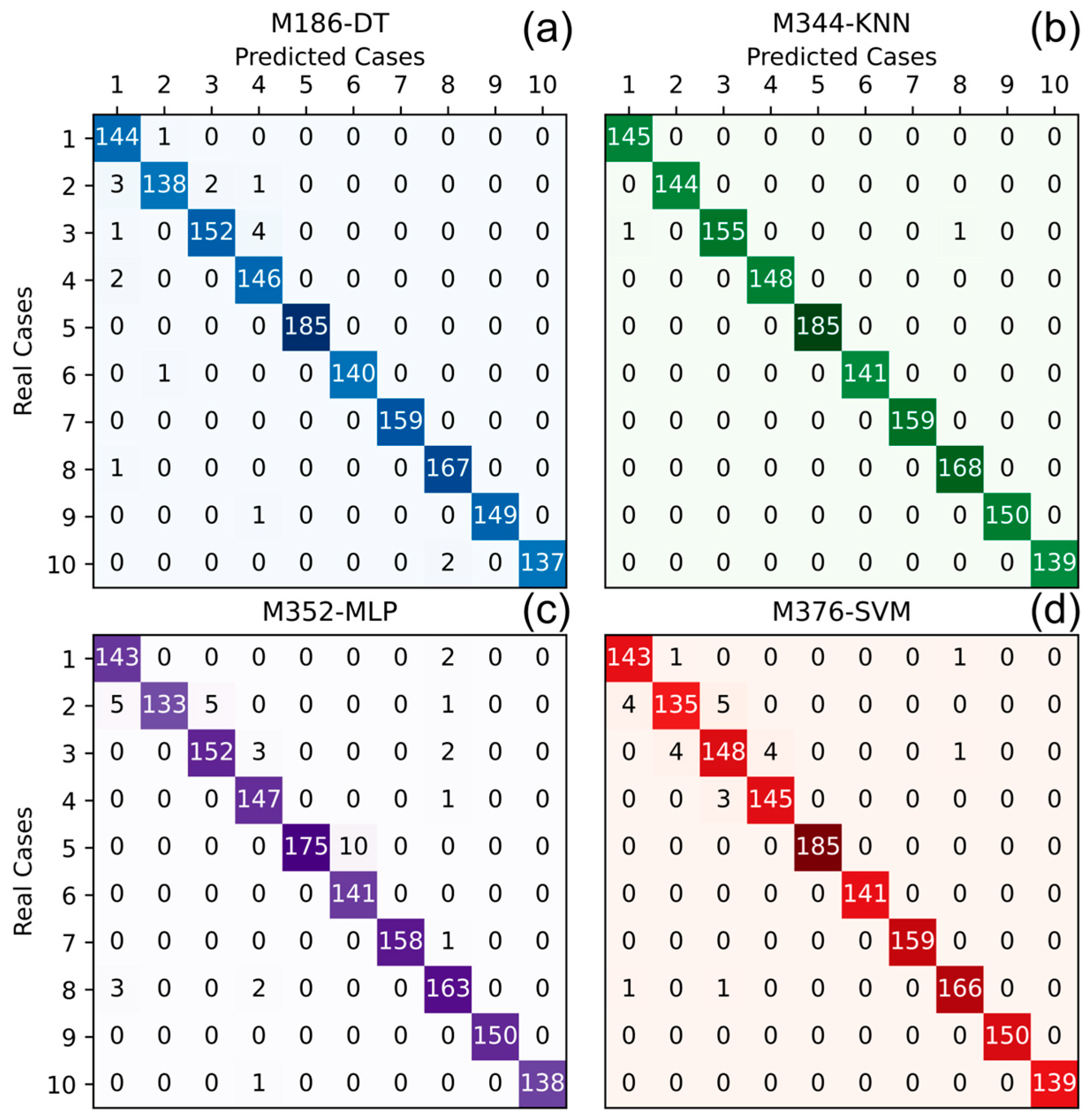
Figure 12 presents the confusion matrices resulting from testing the best machine learning models for each algorithm listed in Table 7. Analyzing Figure 12 reveals that the distribution of tested cases has an overall standard deviation of 8.77%, indicating a balanced dataset. Specifically, Figure 12a illustrates that the M186-DT model experiences classification errors across all cases but demonstrates strong overall performance. In contrast, Figure 12b shows that the model 344-KNN has a lower failure margin, with only 2 cases misclassified, highlighting its exceptional performance. Figure 12c indicates that the M352-MLP model performs well in classifying various cases; however, it ranks below the previously mentioned models due to a higher number of errors in specific classes, such as case 2 and case 5 (Table 2), which correspond to Cracked Tip on WTB bolted to P1 and Cracked Tip on WTB bolted to P2, respectively. Lastly, Figure 12d reveals that the M376-SVM model has good overall performance, but it is noted as the weakest among the four selected models. This model exhibits classification errors with greater dispersion between classes, which could lead to problems in specific categories like case 2 and case 3 (cracked tip on WTB bolted to P1 and cracked mid on WTB bolted to P1).

To evaluate the safety and cost trade-offs for industrial applications, the misclassification rate (MCR) for the best-performing models was calculated, as shown in

Table 9. Misclassification rate.

Case	Misclassification Rate (%)
	M186-DT	M344-KNN	M352-MLP	M376-SVM
1	0.689655	0	1.37931	1.37931
2	4.166667	0	7.638889	6.2500
3	3.184713	1.273885	3.184713	5.732484
4	1.351351	0	0.675676	2.027027
5	0	0	5.405405	0
6	0.70922	0	0	0
7	0	0	0.628931	0
8	0.595238	0	2.97619	1.190476
9	0.666667	0	0	0
10	1.438848	0	0.719424	0
Mean MCR (%)	1.280226	0.127392	2.260617	1.65785

. The MCR is a machine-learning metric that measures the proportion of incorrect predictions made by a classification model, calculated as the total number of incorrect predictions divided by the total number of predictions. A lower MCR indicates a better-performing model [37]. The evaluated cases demonstrated a significantly lower MCR, ranging from 0% to 7.6%. The M186-DT model records a mean MCR of 1.280226% (19 misclassified events out of 1536 evaluated), primarily concentrated in cases 2 and 3. The M344-KNN model shows a mean MCR of 0.127392% (2 misclassified events out of 1536 evaluated), occurring solely in case 2. The M352-MLP model has a mean MCR of 2.260617% (36 misclassified events out of 1536 evaluated), with higher incidences in cases 2, 3, 5, and 8. The M376-SVM model achieves a mean MCR of 1.65785% (25 misclassified events out of 1536 evaluated), focusing on cases 2 and 3. Among these models, the M344-KNN model shows the lowest MCR, making it the most reliable option for critical environments, such as crack detection in WTBs.

Table 10. Analysis of F1-score metrics in macro, micro, and weighted modes.

ML Model ID	Metrics
	F1-Score (Macro) (%)	F1-Score (Micro) (%)	F1-Score (Weighted) (%)
M186-DT	98.725776	98.76302083	98.765499
M344-KNN	99.87186	99.86979167	99.869583
M352-MLP	97.671101	97.65625	97.656611
M376-SVM	98.340148	98.37239583	98.369077

presents the F1-score metrics in macro, micro, and weighted modes. An analysis of these results reveals that the values of the three metrics are consistent across the four models. This consistency indicates the generalizability of the models, demonstrating solid and uniform performance for each class. Additionally, the results suggest that the models are not biased, despite the slight imbalance in the data.

Table 11. Comparison of computational cost.

ML Model ID	Train			Validation			Test
	Ram (MB)	CPU (s@100%)	TFLOPs	Ram (MB)	CPU (s@100%)	TFLOPs	Ram (MB)	CPU (s@100%)	TFLOPs
M186-DT	3.5	0.000001	0.00000006	1.2	0.000000	0.00000002	1.2	0.000000	0.00000002
M334-KNN	18.0	0.14	0.008	6.0	0.05	0.003	6.0	0.05	0.003
M352-MLP	30.0	0.005	0.0003	10.0	0.002	0.0001	10.0	0.002	0.0001
M376-SVM	20.0	0.22	0.013	7.0	0.07	0.004	7.0	0.07	0.004

shows the computational cost of implementing the machine learning models. The M186-DT is the most efficient, with the lowest consumption of RAM and TFLOPs, making it suitable for moderate datasets. In contrast, the M334-KNN and M376-SVM models have the highest costs. In the first model, the reason for these costs is due to its dependence on stored instances, while the reason in the second model is the number of support vectors evaluated. The M352-MLP model is in between, with higher memory usage but fewer operations than models based on KNN and SVM, which keeps it competitive. These results show that the choice of a model should consider not only accuracy, but also the balance between computational cost and expected benefit.

6. Conclusions and Future Work

It was observed that some traditional methods, such as frequency analysis, are difficult to apply when identifying and locating cracks in the blades of operating small WTs. This is due to the numerous disturbances in the phenomenon, the requirement for stable rotation speeds over extended periods, and the high variability of each element’s characteristic frequency spectrum due to its interaction with the system. Therefore, direct implementation of these traditional methods in rotating elements is not recommended.

On the other hand, this comparative study demonstrated that models based on machine learning algorithms and vibration signals perform well in detecting the presence of cracks, identifying the cracked blade, and locating the zone where the crack occurs in the blades of small wind turbines. The KNN models consistently achieve the highest accuracy, even as the sample size increases. The DT and MLP models also perform well but exhibit more variability in their results. Notably, the MLP models demonstrated strong performance, with M352-MLP nearly matching the top performance of KNN. Meanwhile, the DT models maintained solid accuracy, though it was slightly lower than that of KNN. The SVM algorithm has only one model, M376-SVM, which displayed acceptable accuracy but did not surpass the other algorithms and is not among the top performers.

The KNN models are the fastest to train due to their lazy learning approach, resulting in minimal training time. The DT models are moderately fast, with training times depending on their depth and the number of features, typically taking under 2 s. In contrast, the MLP and SVM models are significantly slower and more computationally intensive to train, with the MLP generally having the longest training duration.

The DT models predict outcomes the fastest, typically in under 0.007 s, making them highly suitable for real-time tasks. They can effectively detect the presence of a crack, identify which blade is cracked, and locate the area where the crack occurs. In contrast, the SVM and MLP models have higher, but still acceptable, prediction times, placing them in the intermediate range for speed. The KNN models are highly accurate but have the longest prediction times. This is because KNN performs comparisons with all training data during runtime, resulting in slower predictions, especially as the dataset size increases.

The study presented in this work was developed considering one type of damage out of many. Therefore, an area for improvement is developing more robust models that allow the detection, location, and categorization of the different types of damage that can occur in the blades of small WTs, such as delamination or extreme bending.

The algorithms studied are machine learning approaches for identifying the cracked blade and locating the zone where the crack occurs in the blades of a small wind turbine. These approaches serve as a foundation for future research, where additional variables, such as temperature, humidity, and load variation, can be considered, along with other factors relevant to real-world monitoring environments.

Another area for improvement is integrating the models into a single software package that can provide information to the operator intuitively and seamlessly through a user-friendly interface.

References

1. Stetco, A.; Dinmohammadi, F.; Zhao, X.; Robu, V.; Flynn, D.; Barnes, M.; Keane, J.; Nenadic, G. Machine learning methods for wind turbine condition monitoring: A review. Renew. Energy 2019, 133, 620–635. [Google Scholar] [CrossRef]
2. Sørensen, B.F.; Jørgensen, E.; Debel, C.P.; Jensen, F.M.; Jensen, H.M.; Jacobsen, T.K.; Halling, K.M. Improved Design of Large Wind Turbine Blade of Fiber Composites Based on Studies of Scale Effects (Phase 1)—Summary Report; Risø National Laboratory Report; Risø National Laboratory: Roskilde, Denmark, 2004. [Google Scholar]
3. Song, X.; Xing, Z.; Jia, Y.; Song, X.; Cai, C.; Zhang, Y.; Wang, Z.; Guo, J.; Li, Q. Review on the damage and fault diagnosis of wind turbine blades in the germination stage. Energies 2022, 15, 7492. [Google Scholar] [CrossRef]
4. Wang, W.; Xue, Y.; He, C.; Zhao, Y. Review of the typical damage and damage-detection methods of large wind turbine blades. Energies 2022, 15, 5672. [Google Scholar] [CrossRef]
5. Lu, B.; Li, Y.; Wu, X.; Yang, Z. A review of recent advances in wind turbine condition monitoring and fault diagnosis. In Proceedings of the 2009 IEEE Power Electronics and Machines in Wind Applications, Lincoln, NE, USA, 24–26 June 2009. [Google Scholar]
6. Li, H.; Chen, C.; Wang, T.; Wang, L. Experimental study of stepped-lap scarf joint repair for spar cap damage of wind turbine blade in service. Appl. Sci. 2020, 10, 922. [Google Scholar] [CrossRef]
7. Awadallah, M.; El-Sinawi, A. Effect and detection of cracks on small wind turbine blade vibration using special Kriging analysis of spectral shifts. Measurement 2020, 151, 107076. [Google Scholar] [CrossRef]
8. Yang, X.; Wang, S.; Zhang, W.; Qin, Z.; Yang, T. Dynamic analysis of a rotating tapered cantilever Timoshenko beam based on the power series method. Appl. Math. Mech. 2017, 38, 1425–1438. [Google Scholar] [CrossRef]
9. Huo, Y.; Wang, Z. Dynamic analysis of a rotating double-tapered cantilever Timoshenko beam. Arch. Appl. Mech. 2016, 86, 1147–1161. [Google Scholar]
10. Cao, D.; Gao, Y.; Wang, J.; Yao, M.; Zhang, W. Analytical analysis of free vibration of non-uniform and non-homogenous beams: Asymptotic perturbation approach. Appl. Math. Model. 2019, 65, 526–534. [Google Scholar]
11. Pacheco-Chérrez, J.; Probst, O. Vibration-based damage detection in a wind turbine blade through operational modal analysis under wind excitation. Mater. Today Proc. 2022, 56, 291–297. [Google Scholar]
12. Pacheco-Chérrez, J.; Cárdenas, D.; Delgado-Gutiérrez, A.; Probst, O. Operational modal analysis for damage detection in a rotating wind turbine blade in the presence of measurement noise. Compos. Struct. 2023, 321, 117298. [Google Scholar] [CrossRef]
13. Joshuva, A.; Sugumaran, V. Wind turbine blade fault diagnosis using vibration signals through decision tree algorithm. Indian J. Sci. Technol. 2016, 9, 1–7. [Google Scholar] [CrossRef]
14. Joshuva, A.; Sugumaran, V. Crack detection and localization on wind turbine blade using machine learning algorithms: A data mining approach. Struct. Durab. Health Monit. 2019, 13, 181–203. [Google Scholar] [CrossRef]
15. Sahoo, S.; Kushwah, K.; Sunaniya, A.K. Health monitoring of wind turbine blades through vibration signal using advanced signal processing techniques. In Proceedings of the 2020 Advanced Communication Technologies and Signal Processing (ACTS), Silchar, India, 4–6 December 2020. [Google Scholar]
16. Wang, M.H.; Lu, S.D.; Hsieh, C.C.; Hung, C.C. Fault detection of wind turbine blades using multi-channel CNN. Sustainability 2022, 14, 1781. [Google Scholar] [CrossRef]
17. Chandrasekhar, K.; Stevanovic, N.; Cross, E.J.; Dervilis, N.; Worden, K. Damage detection in operational wind turbine blades using a new approach based on machine learning. Renew. Energy 2021, 168, 1249–1264. [Google Scholar] [CrossRef]
18. Li, Y.; Jiang, W.; Zhang, G.; Shu, L. Wind turbine fault diagnosis based on transfer learning and convolutional autoencoder with small-scale data. Renew. Energy 2021, 171, 103–115. [Google Scholar] [CrossRef]
19. Surucu, O.; Gadsden, S.A.; Yawney, J. Condition Monitoring using Machine Learning: A Review of Theory, Applications, and Recent Advances. Expert Syst. Appl. 2023, 221, 119738. [Google Scholar] [CrossRef]
20. Shehata, A.; Mohammed, O.D. Machine Learning Techniques for Vibration-Based Condition Monitoring—A Review. In Prognostics and System Health Management Conference (PHM); IEEE: Stockholm, Sweden, 2024; pp. 229–234. [Google Scholar]
21. Koutsoupakis, J.; Seventekidis, P.; Giagopoulos, D. Machine learning based condition monitoring for gear transmission systems using data generated by optimal multibody dynamics models. Mech. Syst. Signal Process. 2023, 190, 110130. [Google Scholar] [CrossRef]
22. Raj, K.K.; Kumar, S.; Kumar, R.R.; Andriollo, M. Enhanced Fault Detection in Bearings Using Machine Learning and Raw Accelerometer Data: A Case Study Using the Case Western Reserve University Dataset. Information 2024, 15, 259. [Google Scholar] [CrossRef]
23. Sobhi, S.; Reshadi, M.; Zarft, N.; Terheide, A.; Dick, S. Condition Monitoring and Fault Detection in Small Induction Motors Using Machine Learning Algorithms. Information 2023, 14, 329. [Google Scholar] [CrossRef]
24. Movsessian, A.; García Cava, D.; Tcherniak, D. An artificial neural network methodology for damage detection: Demonstration on an operating wind turbine blade. Mech. Syst. Signal Process. 2021, 159, 107766. [Google Scholar] [CrossRef]
25. Choe, D.E.; Kim, H.C.; Kim, M.H. Sequence-based modeling of deep learning with LSTM and GRU networks for structural damage detection of floating offshore wind turbine blades. Renew. Energy 2021, 174, 218–235. [Google Scholar] [CrossRef]
26. García Márquez, F.P.; Peco Chacón, A.M. A review of non-destructive testing on wind turbines blades. Renew. Energy 2020, 161, 998–1010. [Google Scholar] [CrossRef]
27. She, H.; Li, C.; Zhang, G.; Tang, Q. Statistical investigation on the coupling mode characteristics of a blade-disk-shaft unit. Mech. Based Des. Struct. Mach. 2021, 51, 4237–4254. [Google Scholar] [CrossRef]
28. Sawant, S.U.; Chauhan, S.J.; Deshmukh, N.N. Effect of crack on natural frequency for beam type of structures. AIP Conf. Proc. 2017, 1859, 020056. [Google Scholar] [CrossRef]
29. Xu, J.; Zhang, L.; Li, S.; Xu, J. The influence of rotation on natural frequencies of wind turbine blades with pre-bend. J. Renew. Sustain. Energy 2020, 12, 023303. [Google Scholar] [CrossRef]
30. Hoskoti, L.; Gupta, S.S.; Sucheendran, M.M. Modeling of geometrical stiffening in a rotating blade—A review. J. Sound Vib. 2023, 548, 117526. [Google Scholar] [CrossRef]
31. Xiaohua, T.; Xiaosai, G.; Xinbo, T.; Lijie, W.; Qiu, L.; Baizhou, L. Modal analysis of micro wind turbine blade using COSMOSWorks. Vibroeng. Procedia 2019, 22, 87–92. [Google Scholar] [CrossRef]
32. Nyquist, H. Certain topics in telegraph transmission theory. Trans. Am. Inst. Electr. Eng. 1928, 47, 617–644. [Google Scholar] [CrossRef]
33. Abhishiktha, T.; Kishore, V.T.; Dipankur, S.; Indraja, V.; Krishna, V. A review on small scale wind turbines. Renew. Sustain. Energy Rev. 2016, 56, 1351–1371. [Google Scholar] [CrossRef]
34. IEC 61400-2:2013; Wind turbines—Part 2: Small wind turbines. International Electrotechnical Commission: Geneva, Switzerland, 2013.
35. Tang, Y.; Chang, Y.; Li, K. Applications of K-nearest neighbor algorithm in intelligent diagnosis of wind turbine blades damage. Renew. Energy 2023, 212, 855–864. [Google Scholar] [CrossRef]
36. Vives, J. Monitoring and Detection of Wind Turbine Vibration with KNN-Algorithm. J. Comput. Commun. 2022, 10, 1–12. [Google Scholar] [CrossRef]
37. Zhou, X.; Wang, X.; Hu, C.; Wang, R. An analysis on the relationship between uncertainty and misclassification rate of classifiers. Inf. Sci. 2020, 535, 16–27. [Google Scholar] [CrossRef]
Figure 1. Segment of 500 samples of the unprocessed vibration signal acquired from WTB bolted to P1 on the hub: (a) Case 1, (b) Case 2, (c) Case 3, and (d) Case 4.
Ai 06 00242 g001
Figure 2. Normalized time series signals from WTB bolted to P1 on the hub: (a) Case 1, (b) Case 2, (c) Case 3, and (d) Case 4.
Ai 06 00242 g002
Figure 3. Frequency spectra of the preprocessed vibration signals measured on (a1) P1 of case 1, (b1) P2 of case 1, (c1) P3 case 1, (a2) P1 of case 2, (b2) P2 of case 2, (c2) P3 of case 2, (a3) P1 of case 3, (b3) P2 of case 3, (c3) P3 of case 3, (a4) P1 of case 4, (b4) P2 of case 4, (c4) P3 case 4, (a5) P1 of case 5, (b5) P2 of case 5, (c5) P3 case 5, (a6) P1 of case 6, (b6) P2 of case 6, (c6) P3 case 6, (a7) P1 of case 7, (b7) P2 of case 7, (c7) P3 case 7, (a8) P1 of case 8, (b8) P2 of case 8, (c8) P3 case 8, (a9) P1 of case 9, (b9) P2 of case 9, (c9) P3 case 9, (a10) P1 of case 10, (b10) P2 of case 10, and (c10) P3 case 10.
Ai 06 00242 g003
Figure 4. DFT of signal samplings of WTB bolted to P1 of the hub: (a) Case 1, (b) Case 2, (c) Case 3, and (d) Case 4.
Ai 06 00242 g004
Figure 5. Methodology of this comparative study.
Ai 06 00242 g005
Figure 6. (a) Frontal view of the test bench diagram, (b) lateral view of the test bench diagram, and (c) data acquisition system implemented on the test bench.
Ai 06 00242 g006
Figure 7. WTB sections.
Ai 06 00242 g007
Figure 8. Dimensions of the WTBs used on the experimental tests: (a) WBT healthy, (b) WTB with cracked tip, (c) WTB with cracked mid, and (d) WTB with cracked root.
Ai 06 00242 g008
Figure 9. Electronic diagram of the DAS for one accelerometer.
Ai 06 00242 g009
Figure 11. Results of metrics calculated during training and fitting of the top 20 best-performing machine learning models for datasets of: (a) 500 samples, (b) 1000 samples, and (c) 5000 samples.
Ai 06 00242 g011
Figure 12. Confusion matrices obtained during the test of the model: (a) M186-DT, (b) M344-KNN, (c) M352.MLP, and (d) M376-SVM.
Ai 06 00242 g012