Article

Effective Hybrid Structure Health Monitoring through Parametric Study of GoogLeNet

Department of Civil, Construction and Environmental Engineering, North Dakota State University, Fargo, ND 58104, USA
*
Author to whom correspondence should be addressed.
AI 2024, 5(3), 1558-1574; https://doi.org/10.3390/ai5030075
Submission received: 8 July 2024 / Revised: 20 August 2024 / Accepted: 22 August 2024 / Published: 30 August 2024

Abstract

:
This paper presents an innovative approach that utilizes infused images from vibration signals and visual inspections to enhance the efficiency and accuracy of structure health monitoring through GoogLeNet. Scrutiny of the structure of GoogLeNet identified four key parameters, and thus, the optimization of GoogLeNet was completed through manipulation of the four key parameters. First, the impact of the number of inception modules on the performance of GoogLeNet revealed that employing eight inception layers achieves remarkable 100% accuracy while requiring less computational time compared to nine layers. Second, the choice of activation function was studied, with the Rectified Linear Unit (ReLU) emerging as the most effective option. Types of optimizers were then researched, which identified Stochastic Gradient Descent with Momentum (SGDM) as the most efficient optimizer. Finally, the influence of learning rate was compared, which found that a rate of 0.001 produces the best outcomes. By amalgamating these findings, a comprehensive optimized GoogLeNet model was found to identify damage cases effectively and accurately through infused images from vibrations and visual inspections.

1. Introduction

Structural health monitoring systems have always required the detection of structural deficiencies like corrosion, reduction in elasticity, or cracks. For a few decades, visual inspection by skilled professionals has been the primary method of identifying structural problems. This method is often time-consuming, risky, and expensive. As a result, researchers are becoming increasingly interested in computer-vision-based sensors for structural damage detection due to their great benefits over manual visual assessment. These sensors enable the use of appropriately calibrated thresholds in image processing operations like edge detection and crack identification.
The detection of structural defects, particularly cracks, is currently achieved using two basic image processing techniques: sequential image processing and image binarization. Images can provide a sufficient range of information [1]. Liu [2] suggested an image binarization technique that was accurate enough to find cracks. The sequential image processing technique was used to successfully identify cracks in photographs of concrete surfaces by Ebrahimkhanlou [3]. However, the majority of the edge detection techniques through various filters, including Roberts, Prewitt, Sobel, and Gaussian, have been used in vision-based fracture detection approaches for concrete structures [4]. These approaches are typically time-consuming and only capable of detecting the presence of cracks in a picture; they cannot assess the severity of cracks directly.
Recent research aimed to categorize and analyze structural defects like cracks and corrosion using new deep learning algorithms to overcome the shortcomings of vision-based crack detection methods. A CNN method was suggested by Rawat and Wang [5] for classifying images. With the use of a Nave Bayes data fusion approach, Chen and Jahanshahi [6] proposed a CNN-based fracture detection system and extracted cracks from video frames recorded for a structure at pixel-level precision. Dorafshan et al. [7] suggested a quicker CNN model with picture binarization. To identify and locate cracks, Soloviev et al. [8], Li et al. [9], Tong et al. [10], and Fan et al. [11] created deep CNN models to identify cracks and determine their sizes.
On the other hand, dynamic properties of a structure, such as its natural frequency, damping ratio, and mode shape, may also be utilized to evaluate the health of the structure and determine where damage has occurred. Structural degradation will alter the mass and stiffness distributions of structures, changing their dynamic properties [12,13,14]. Vibration-based structural damage detection methods with system identification could be utilized to establish correlations between the vibration features and the damage information [15,16,17], except natural frequencies are not sensitive to minor damage and could be easily contaminated by environmental factors. Following a similar thought process as the image-based structural condition assessment, some researchers also investigated identifying damage through deep learning models with vibration data inputs. Lin, Nie, and Ma [18] suggested a deep learning technique based on a CNN that has three maximum pooling layers and six convolutional layers. After that, the raw vibration data from a finite element beam were used to train this CNN-based system, and the damage was effectively identified with a high accuracy rate of 94.57%. Applying the CNN-based method, some researchers were able to find the damage created by losing bolts of a steel truss with great accuracy [19,20] and by using wireless sensor network inputs [21].
Artificial intelligence (AI) plays a transformative role in structural health monitoring by enabling the more accurate, efficient, and proactive management of infrastructure. Through advanced algorithms and machine learning techniques, AI can analyze vast amounts of data from sensors embedded in structures—such as bridges, buildings, and dams—to detect early signs of potential issues. This capability allows for the real-time assessment of structural integrity, identifying anomalies or patterns that might indicate wear, stress, or damage. Many researchers applied artificial intelligence and machine learning in the optimization and monitoring of construction activities [22,23,24]. Artificial intelligence models can assist construction safety monitoring and construction activity scheduling tremendously, which has helped to reduce construction accidents and shorten construction time [25].
In this research, our primary objective revolves around enhancing the performance of GoogLeNet when integrating fusion images derived from different vibration data and damage images. By merging these distinct data, it can create a robust and effective framework capable of detecting and diagnosing structural damage with heightened accuracy and efficiency. Through this fusion approach, we endeavor to exploit the complementary information present in both types of data, leveraging the spatial and spectral characteristics of damage images along with the dynamic signs captured by vibration data. At the same time, we aim to optimize GoogLeNet’s architecture to seamlessly integrate these heterogeneous inputs. Based on the above rationale, the manuscript is organized as follows: In Section 1, the literature review and background on structural health monitoring using fused data from different sources is summarized. In Section 2, the detailed GoogLeNet and its potential in SHM are included. In Section 3, a parametric study was conducted to identify the most efficient GoogLeNet, and their performance on fused data was compared. Section 4 provides the conclusion of the study.

2. Research Methodology

2.1. Deep Learning-Based Damage Detection Using the Fusion of Vibration Data and Defect Images

Typically, there are three main sections in a convolutional neural network to identify the structural damage through fusion data, as shown in Figure 1, including (1) data set collection, (2) CNN model training, and (3) validation and prediction. Vibrations at measure points under dynamic loads are first obtained in the ABAQUS model and converted to images. These vibration images are then paired with structure damage images to serve as inputs to the GoogLeNet model.
After that, the paired images are classified as different patterns according to different damage cases and are divided into three groups randomly, 70% of which are for training, 15% of which are for validation, and 15% of which are for testing.
The three layers that form the suggested CNN model are the convolution layer, pooling layer, and fully connected layer. Artificial neurons are stacked in these layers according to three dimensions: depth, width, and height. The damage identification part uses the paired images at various locations on the structure, which is represented as a two-dimensional matrix, as its input data. The CNN model then iteratively goes across each layer to convert the two-dimensional matrix into a one-dimensional vector matching to the category.
The fundamental component of the CNN model is the convolutional layer. Each convolutional block has variables that can be learned, such as biases and weights (filters). The filter’s depth is the same, but its width and height are spatially less than the input. For instance, since the RGB image contains three layers, the convolutional layer should have three depths to examine each of the three levels separately. The previous layer’s features are convolved using filters to create the output, which is then mapped to the new features in the current layer using the activation function. The convolutional layer for a pixel used the following equation:
C x y = σ i = 1 h j = 1 w k = 1 d f i j k X x + i , y + j 1 , k + b
where X is the input vector of intensity values of the image, b is the bias vector, σ is the activation function, and f is the weight matrix, and where h and w are the filter’s sizes and d is the number of input channels.
Figure 2 illustrates the convolution process on a randomly chosen 4 × 4 matrix. A 3 × 3 matrix is selected as the filter which is generated randomly at the initial state and updated from the model by a backward propagation algorithm.
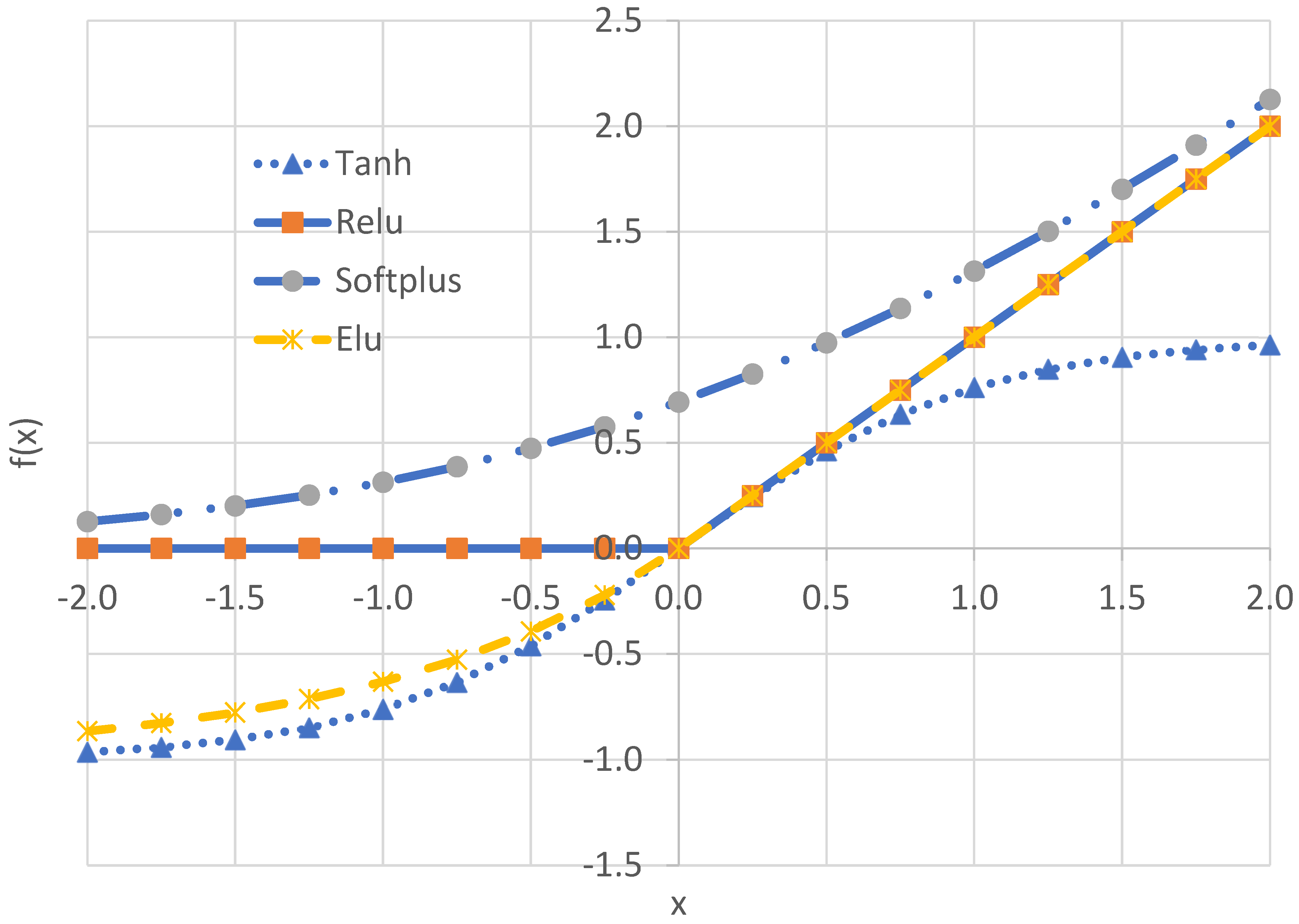
Four sub-arrays of the same size are created by sliding along the input matrix’s width and height with a stride of 1. Each sub-array is multiplied by the filter matrix. The output value, which is the result of adding the multiplied values and the bias, is then obtained. Because of the stride, the output is smaller than it was in the prior layer. The nonlinear activation function, which is used to add nonlinearity to the network, comes after the convolution layer. Rectified linear unit (ReLU), softplus, tanh, and Elu are some of the activation functions that are most frequently employed in neural networks. Their respective functions are expressed as follows:
f x = max 0 , x
f x i = l o g ( 1 + e x )
f x = e x e x e x + e x
f x = max e x 1 , x
where f(x) is the function that could represent the probability of firing or activating the neurons in the next inception layer and x denotes the state of the current neuron. These functions are shown in Figure 3.
The optimizer is considered one of the crucial components of the training process. The optimizer is responsible for adjusting the parameters of the network during the training process to minimize the loss function. Many optimizers can be used in training, such as stochastic gradient descent (Sgdm), adaptive momentum estimation (Adam), and root mean square propagation (RmsProp). The choice of optimizer can significantly impact the convergence speed and performance of the model in the task at hand. Therefore, selecting an appropriate optimizer and tuning its parameters are essential steps in the development of a successful CNN model.
The final layer before the network’s output layer is the completely connected layer. All of the neurons in this layer are connected to the features created in the layer before. The generated features are transformed into corresponding categories in this layer via weights and biases. The equation of the output yi is shown as follows:
y l = σ y l 1 w + b
where σ is the activation function; w and b represent the weights and bias vectors in this layer, respectively; i is the iteration step.

2.2. Transfer Learning Method Used

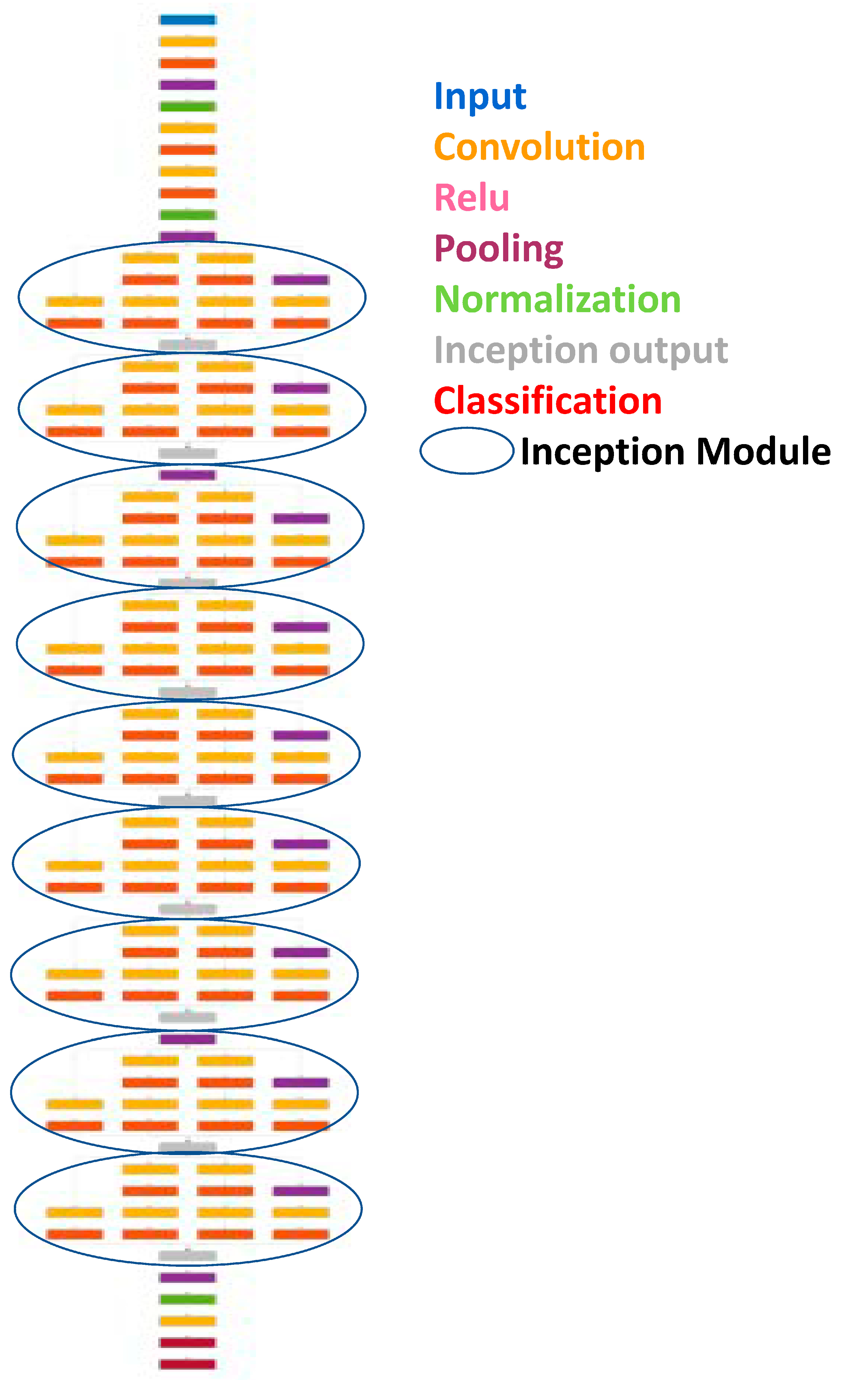
GoogLeNet is a particular kind of convolutional neural network built on the inception model. Using inception modules, the network is able to select among a variety of convolutional filter sizes for each block. These modules are stacked on top of one another using a convolutional network, which occasionally uses max-pooling layers with stride 2 to cut the grid’s resolution in half.
GoogLeNet has been trained on over a million images and can classify images into 1000 object categories (such as keyboards, coffee mugs, pencils, and many animals). The network has learned rich feature representations for a wide range of images. The network takes an image as input with 224 × 244, and then outputs a label for the object in the image together with the probabilities for each of the object categories.
The GoogLeNet architecture consists of 22 layers (27 layers including pooling layers) which are tabulated in Table 1, and part of these layers are a total of nine inception modules, as shown Figure 4. Each red circle represents an inception layer.

2.3. Gramian Angular Field (GAF)

The GAF algorithm was developed in the area of time series data to preserve characteristics when encoding 1D time series into 2D images. The two methods that can be used to complete GAF are the Gramian angular difference field (GADF) and the Gramian angular sum field (GASF). The vibration data are X = {x1, x2, …, xi, …, xn}, where n is the total number of displacement points and xi is the value of the displacement. The spectral data must first be normalized, scaled to the range of [0, 1], and recorded as xi,n.
x i n = x i m i n X m a x X m i n X
Next, using the following formula, the 1D spectral sequence in the Cartesian coordinate system is converted to a polar coordinate system:
φ = a r c c o s x i , n
Time dependence is maintained in the Gramian matrix. The time dimension is encoded into the matrix’s geometry because time grows as the position shifts from the upper left corner to the lower right corner. Equation (8) shows that the converted angle ϕ has a value range of [0, π] and that the cosine value decreases monotonically within this range. The increase in time corresponds to the radius in the polar coordinate system, while xi in each Cartesian coordinate system responds to the angle value in the polar coordinate system, and the corresponding bending takes place between various angle points on the polar coordinate circle. Thus, the Gramian angular summation field (GASF) can be obtained by computing the cosine value of the sum of angles between various points, as follows (Equation (9)):
G A S F = cos φ i + φ j = cos φ 1 + φ 1 cos φ 1 + φ n cos φ n + φ 1 cos φ n + φ n = x ˜ i . x ˜ j 1 x ˜ i 2 1 x ˜ j 2 = X ˜ T X ˜ 1 X ˜ 2 T 1 X ˜ 2
where I is the unit vector. X ˜ i is the normalized vibration data, and φ is the angle of the point.
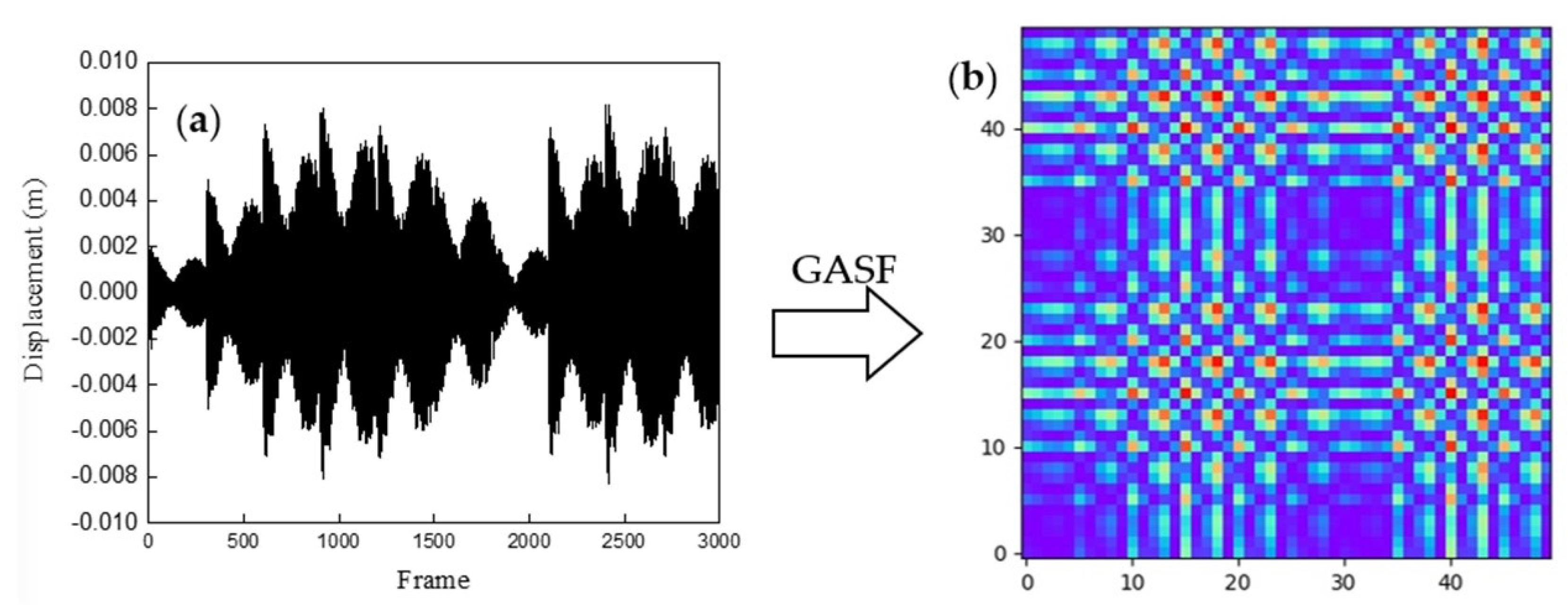
An example employing vibration data from the steel truss model’s ABAQUS model is shown in Figure 5a. The suggested GASF is used to transform the vibration into images, and the resulting images include several distinct elements, including the lines and points that are indicated in Figure 5b. Red color indicates higher value locations while blue colors stand for the low value locations and green colors stand for the intermediate value locations.

3. Case Study and Validation

3.1. Data Collection through ABAQUS Modeling

The ABAQUS truss model is shown in Figure 6. In this study, the truss comprises eight spans and nine measurement points. There are 16 scenarios in all, and Table 2 displays the locations of the damage in each case. f represents the front face and t represents the top face of the truss. T, m, and r represent the top element, middle element, and right element, respectively. For example, for case number 8, the sloping rod on the front face is damaged by reducing 30% of its elastic modulus. Case no. 5 represents the damage on the top element of the front face at the fourth span of the truss.
Dynamic load is applied at the mid-point of the truss, and dynamic displacement data are collected at the specified measurement point. Figure 7 shows the dynamic displacement at the MP1 location for damage case 2.

3.2. Structural Evaluation Using a Novel Deep Learning-Based Method with Both Defect Image and Vibration Data

As seen in Figure 8, pictures of structural defects at measurement points can be obtained using a camera or UAV. An image-based displacement sensor, on the other hand, gathers the structure’s vibration data. These one-dimensional vibration data are further converted into two-dimensional images using the above GASF algorithm. These two groups of images are then paired to provide input data for the deep learning model.

3.3. Gramian Angular Field

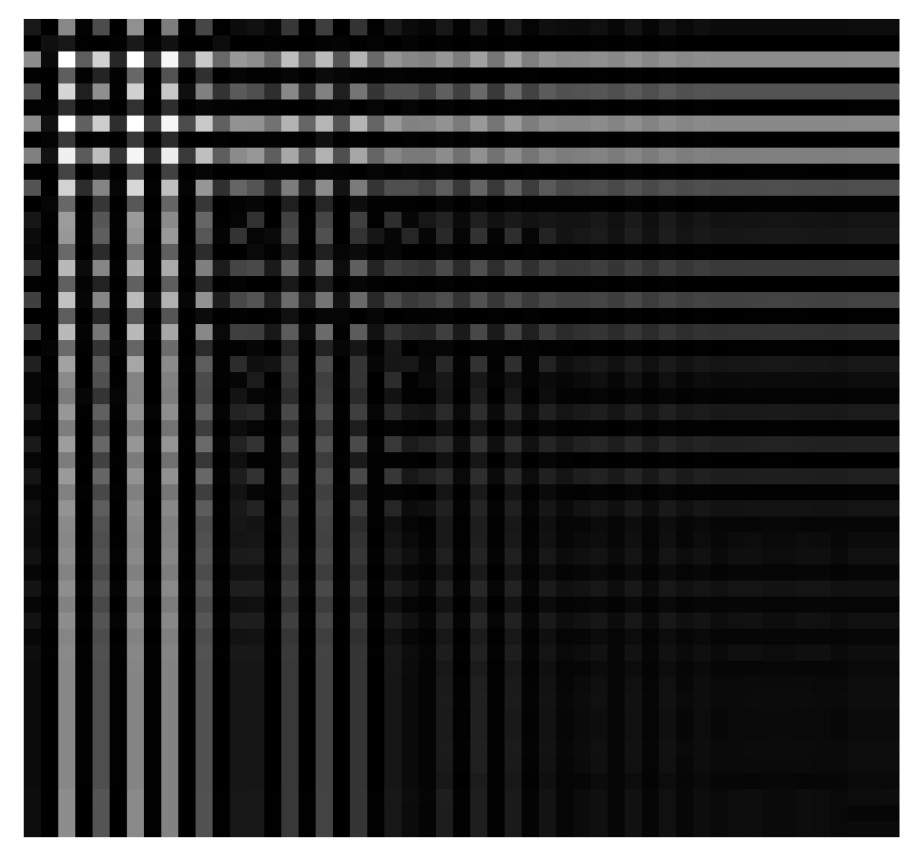
Without losing any features, 1D time series were encoded into 2D images using the GASF algorithm. An example using vibration data from the steel truss model in ABAQUS is presented in Figure 9.

3.4. Paired Images

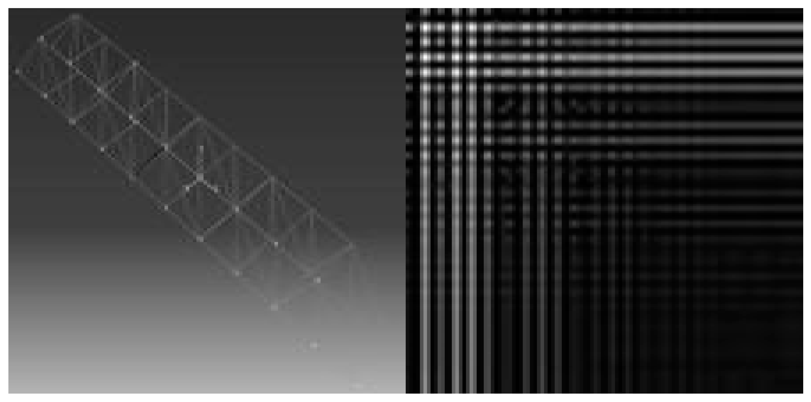
Images of the defected truss for each case were taken, and vibration signals at each sensor location were recorded and converted to images using GASF. In addition, 288 paired images with sizes of 224 × 224 were obtained for the truss. Figure 10 shows a paired image of the truss and the image obtained by GASF.

4. Results of the Proposed Method

In order to validate this procedure, vibrations from the steel truss ABAQUS models were translated into images using GASF. In the ABAQUS model of the steel truss, there were sixteen sets of integrated images with various faults (30% reduction in modulus of elasticity at different locations) and damage locations (no damage, No. 3 damage, and No. 5 damage). There were 128 images in total and 9 images for each group of the case study.

4.1. Results of Model Training, Validation, and Prediction

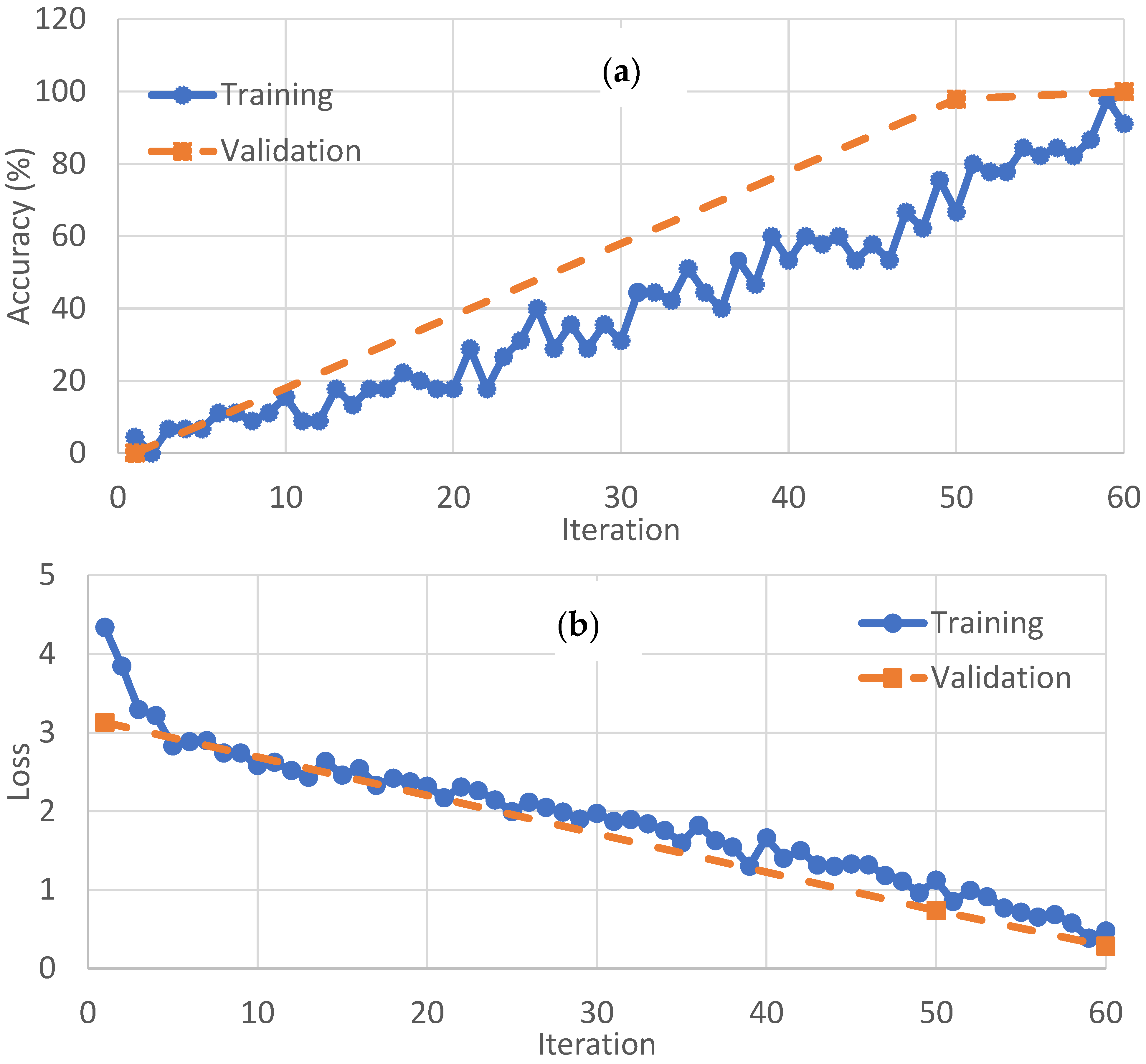
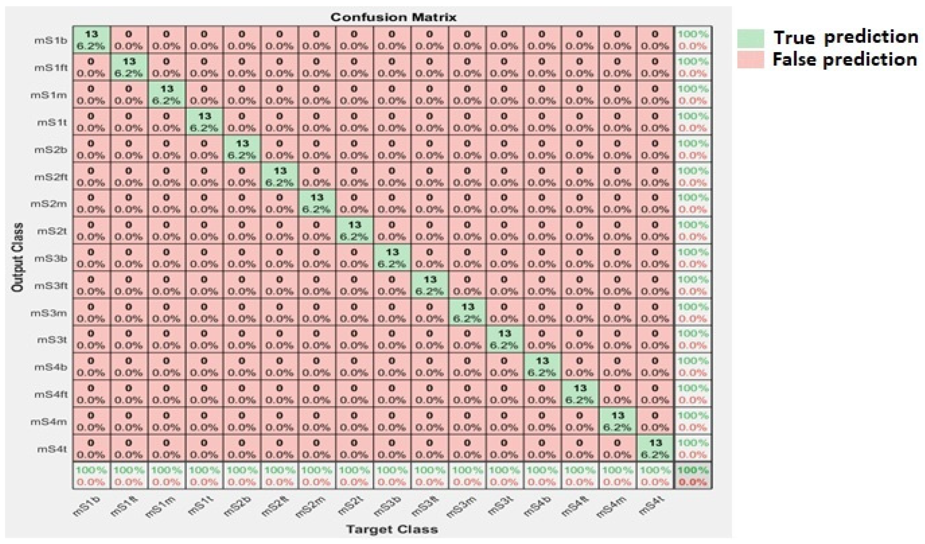
The above-described process resulted in satisfactory outputs. For the damage truss cases at different locations with the combination of GASF images converted from vibration data, the accuracy and the loss of the training and validation of the GoogLeNet model are shown in Figure 11, which gives 100% accuracy. Figure 12 is shown the confusion matrix of using infused images as input data for the model. The solid line indicates the training accuracy while the dash line indicates the validation accuracy.

4.2. Effect of the Number of Inception Layers

Inception modules are important in feature detection. The training accuracy of GoogLeNet with different numbers of inception modules is shown in Figure 13. The results demonstrated the efficiency of the original configuration with nine inception layers in capturing intricate characteristics and patterns of the input data, with perfect 100% accuracy. Similarly, when reducing the number of inception layers to eight, the model maintained its high accuracy of 100%, indicating the robust performance of the GoogLeNet model even with a slightly simplified architecture. On the other hand, as the number of layers decreased further, the accuracy of the GoogLeNet model fluctuated. With seven layers, the accuracy dropped to 70%, suggesting a sharp decrease in performance due to its reduced capacity to capture intricate details. A further reduction to six layers led to a decrease in accuracy to 57%, highlighting the diminishing capacity of the model to learn and generalize the input data patterns. Overall, these results demonstrate the intricate relationship between model depth and performance, emphasizing the importance of striking the right balance between complexity and generalization capacity.

4.3. Effect of Learning Rate

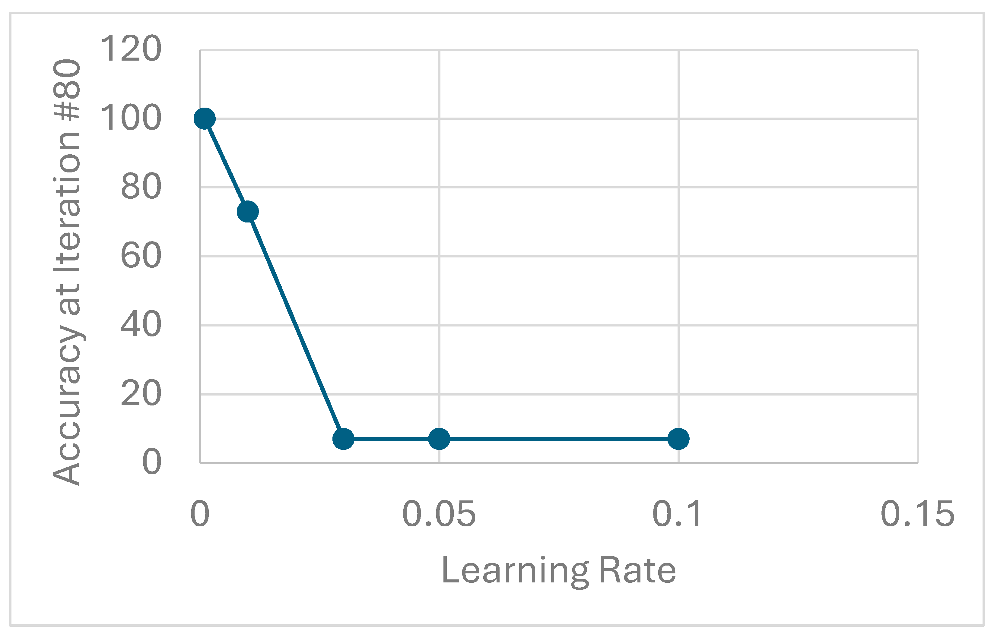
Model accuracy is affected by the variation in learning rates, as shown in Figure 14. When utilizing a learning rate of 0.001, the model achieved 100% accuracy, showing the effectiveness of a smaller learning rate and steady convergence. However, when the learning rate was increased to 0.01, the accuracy dropped to 73%. While still respectable, this decrease suggests that the higher learning rate might have caused oscillations around the optimal solution or even led to divergence in some cases, hindering the model’s ability to converge effectively. Subsequently, employing a learning rate of 0.03 or more resulted in accuracy of a mere 7%, indicative of overshooting and divergence, as the excessively large learning rate likely caused the optimization process to become saturated and unstable, preventing the model from learning meaningful representations. These results underscore the critical role of learning rate selection in optimizing model performance, emphasizing the need for careful tuning to strike a balance between convergence speed and stability.

4.4. Effect of Activation Function

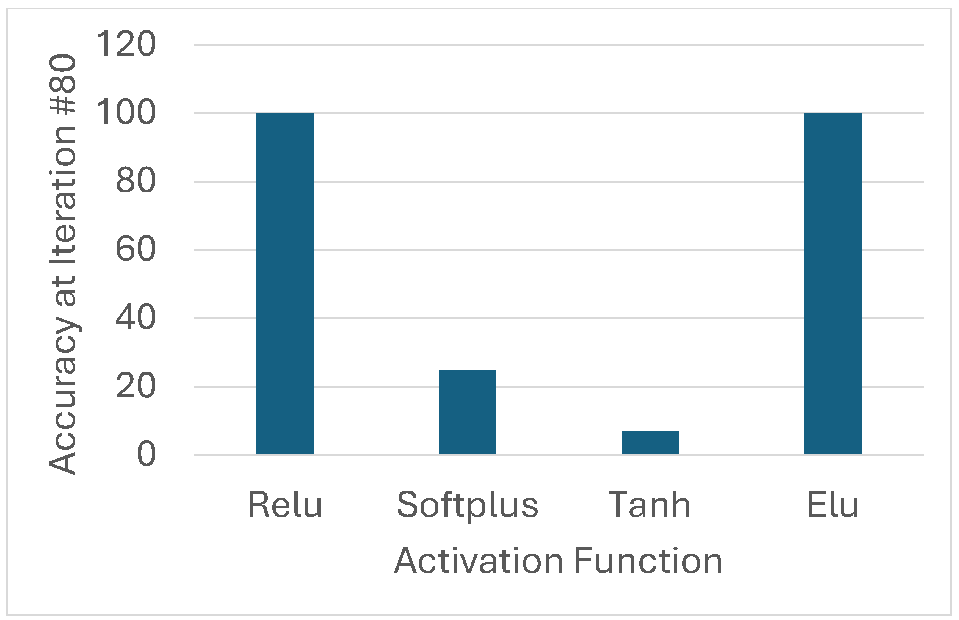
Figure 15 shows the effect of different activation functions, which gave different accuracies in model training. When employing Rectified Linear Unit (ReLU), the model achieved perfect 100% accuracy, indicating its effectiveness in promoting nonlinearity and mitigating the vanishing gradient problem, thus enabling robust learning. Similarly, when using Exponential Linear Unit (ELU), the model again attained 100% accuracy. ELU’s capability to handle negative values might have facilitated smoother gradients and enhanced model convergence. Softplus activation function resulted in 25% accuracy, likely due to its gradual gradient and lack of a strict zero threshold, which might have hindered the model’s ability to capture complex patterns effectively. However, when employing Hyperbolic Tangent (tanh), the accuracy dropped to 7%. Tanh’s saturating nature might have led to vanishing gradients, impeding the model’s learning process and hindering its performance. In general, the divergent outcomes underscore the significant impact of activation functions on model learning dynamics and performance.

4.5. Effect of Different Optimizers

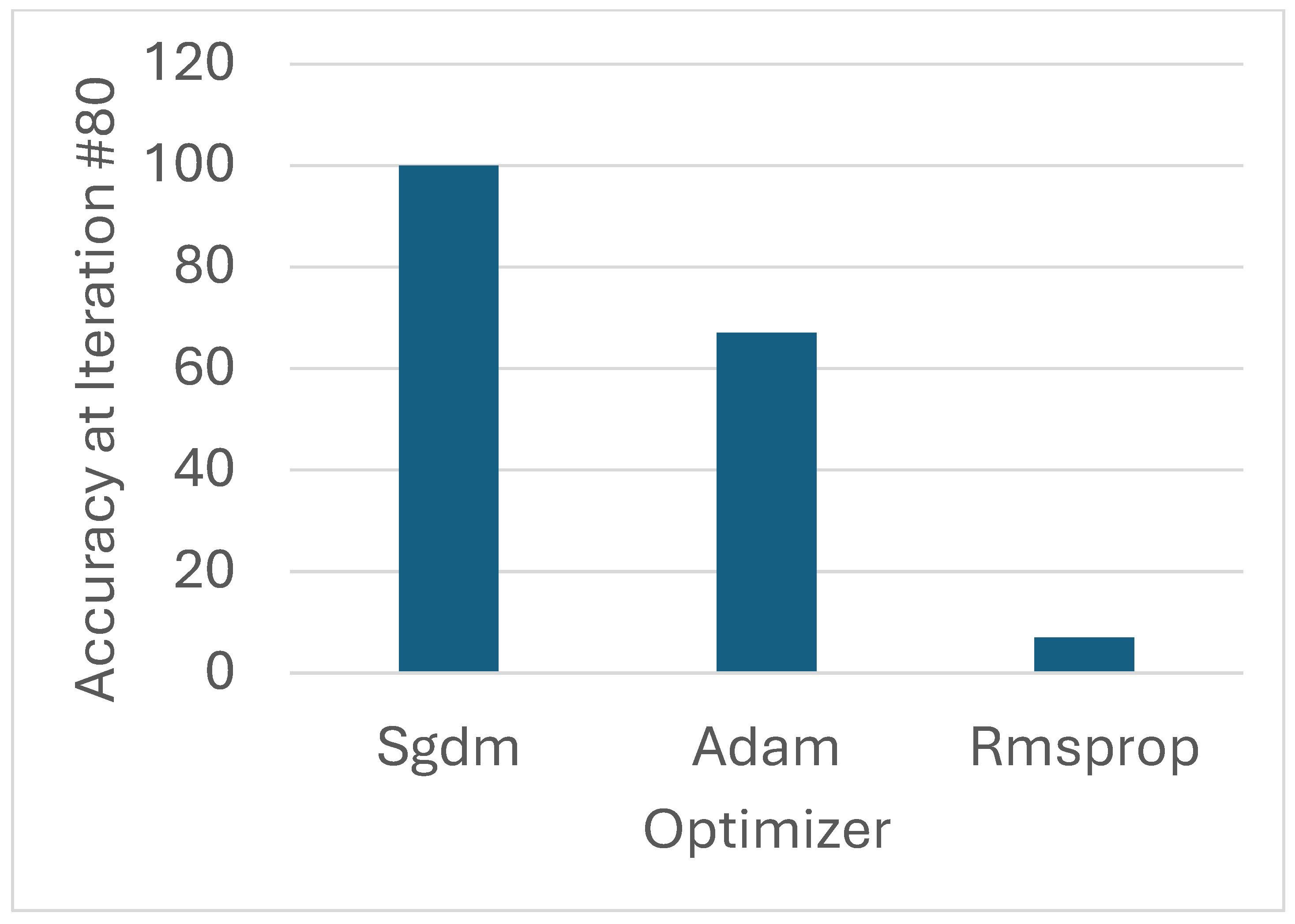
Training GoogLeNet with different optimizers yielded varying accuracies, as shown in Figure 16. When trained with Stochastic Gradient Descent with Momentum (SGDM), the model achieved remarkable 100% accuracy, showing its ability to converge quickly and effectively optimize the parameters. However, when trained with Adam optimizer, the accuracy dropped to 67%. Adam optimizer, while popular for its adaptability to various datasets, might have struggled to navigate the complex architecture of GoogLeNet effectively, leading to suboptimal results. On the other hand, training with RMSprop yielded accuracy of a mere 7%, indicating its limitations in handling the intricate nuances of GoogLeNet’s architecture. RMSprop, though robust in handling non-stationary objectives, might have encountered difficulties in maintaining the necessary momentum for convergence in this scenario. Overall, the varying performances highlight the sensitivity of deep learning models to the optimizer selection, emphasizing the importance of careful experimentation and tuning to achieve optimal results.

4.6. Effect of Training Data Set Sizes

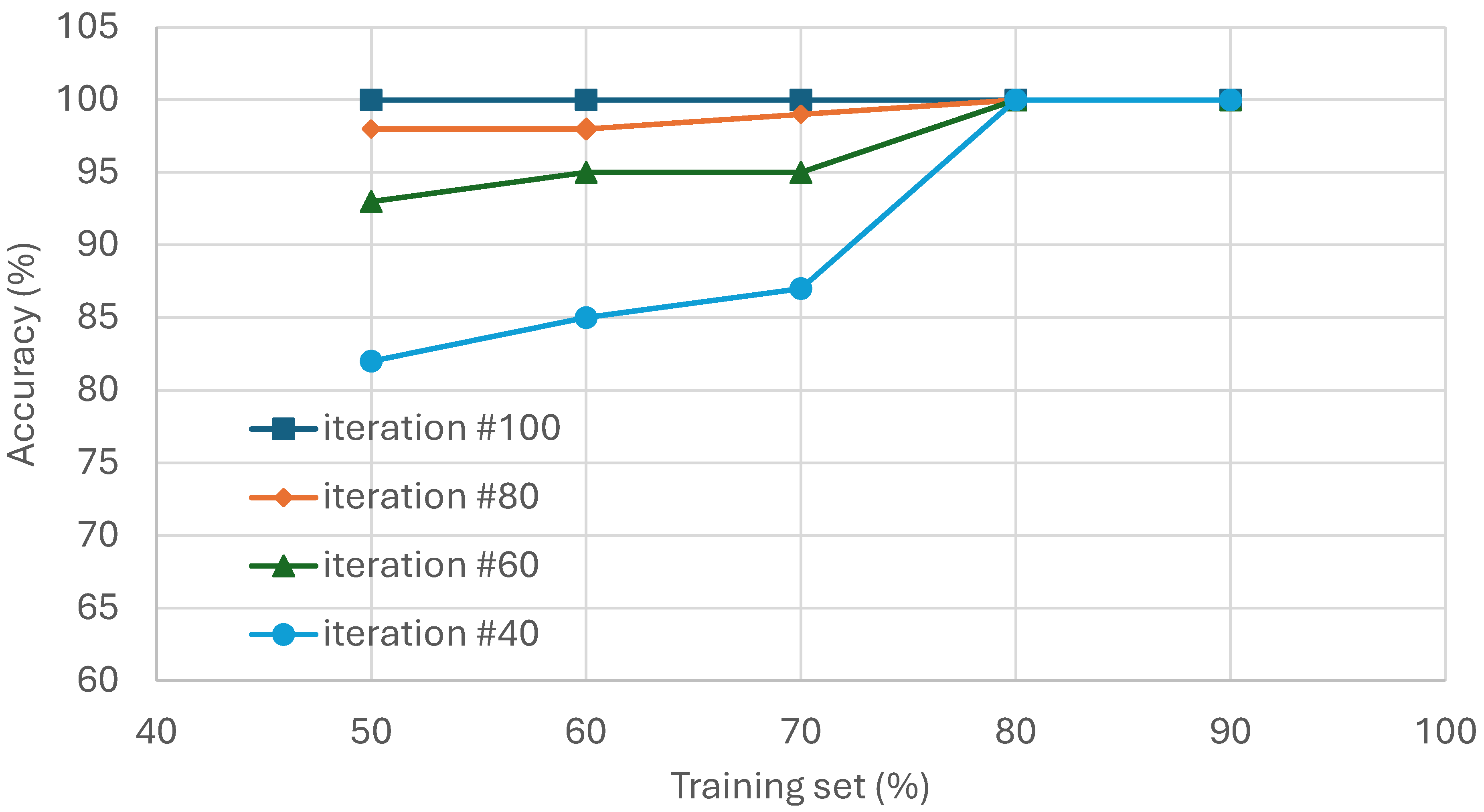
The effect of training data set sizes was studied and is shown in Figure 17. Here, 50%, 60%, 70%, 80%, and 90% of the total data were used as the training set, while the rest of the data were split equally into the validation and test sets. The accuracies at different iteration steps are also included in the figure. From the results shown, one can see the GoogLeNet model converges earlier when a larger portion of the data is used as the training data set. And the accuracy at the 80th iteration converges for all training data sizes and the accuracy at the 80th iteration can be used as a reliable criterion to analyze the effect of different hyperparameters.

5. Conclusions

In conclusion, this paper aimed to enhance the efficiency and accuracy of a new structure health monitoring method that utilizes infused images from vibrations and visual inspections through a parametric study of the GoogLeNet architecture. By leveraging deep learning techniques, this study sought to optimize the performance of the network by manipulating four key parameters: the number of inception modules, activation function, optimizer, and learning rate. Notably, employing eight inception modules achieved superior performance with less computational time compared to using nine inception layers. Additionally, the Rectified Linear Unit (ReLU) activation function emerged as the most effective choice, while the Stochastic Gradient Descent with Momentum (SGDM) optimizer and a learning rate of 0.001 showed superior performance. By integrating these findings, an efficient and effective new structural health monitoring method was found through optimization of the GoogLeNet model. This study not only provides valuable insights into structural health monitoring techniques but also underscores the importance of deep learning models to achieve superior model performance.
In future work, case studies with real structures of different damage conditions will be conducted. The effects of paired image sizes, other hyperparameters of the GoogLeNet model, and different sizes of training data set are not studied in this manuscript, and we hope to explore them.

Author Contributions

Conceptualization, S.A.-Q. and M.Y.; methodology, S.A.-Q.; validation, S.A.-Q. and M.Y.; formal analysis, S.A.-Q. and M.Y.; investigation, S.A.-Q.; resources, M.Y.; data curation, S.A.-Q.; writing—original draft preparation, S.A.-Q.; writing—review and editing, M.Y.; visualization, S.A.-Q.; supervision, M.Y.; project administration, M.Y.; funding acquisition, M.Y.. All authors have read and agreed to the published version of the manuscript.

Funding

The research is funded by the North Dakota NASA EPSCoR Grant, with the Grant number 36937.

Institutional Review Board Statement

Not applicable.

Informed Consent Statement

Not applicable.

Data Availability Statement

Dataset available on request from the authors.

Acknowledgments

We thank our colleagues from North Dakota State University who provided insight and expertise that greatly assisted the research, although they may not agree with all of the interpretations/conclusions of this paper.

Conflicts of Interest

The authors declare no conflict of interest.

References

  1. Almousa, M.; Olusegun, T.; Lim, Y.; Al-Zboon, K.; Khraisat, I.; Alshami, A.; Ammary, B. Chemical recovery of magnesium from the Dead Sea and its use in wastewater treatment. J. Water 2024, 14, 229–243. [Google Scholar] [CrossRef]
  2. Liu, Y.; Cho, S.; Spencer, B.F., Jr.; Fan, J. Automated assessment of cracks on concrete surfaces using adaptive digital image processing. Smart Struct. Syst. 2014, 14, 719–741. [Google Scholar] [CrossRef]
  3. Ebrahimkhanlou, A.; Farhidzadeh, A.; Salamone, S. Multifractal analysis of crack patterns in reinforced concrete shear walls. Struct. Health Monit. 2016, 15, 81–92. [Google Scholar] [CrossRef]
  4. Yang, X.; Li, H.; Yu, Y.; Luo, X.; Huang, T.; Yang, X. Automatic pixel-level crack detection and measurement using fully convolutional network. Comput.-Aided Civ. Infrastruct. Eng. 2018, 33, 1090–1109. [Google Scholar] [CrossRef]
  5. Rawat, W.; Wang, Z. Deep Convolutional Neural Networks for Image Classification: A Comprehensive Review. Neural Comput. 2017, 29, 2352–2449. [Google Scholar] [CrossRef]
  6. Chen, F.-C.; Jahanshahi, M.R. NB-CNN: Deep Learning-Based Crack Detection Using Convolutional Neural Network and Naïve Bayes Data Fusion. IEEE Trans. Ind. Electron. 2018, 65, 4392–4400. [Google Scholar] [CrossRef]
  7. Dorafshan, S.; Maguire, M.; Hoffer, N.V.; Coopmans, C. Fatigue Crack Detection Using Unmanned Aerial Systems in Under-Bridge Inspection; Idaho Transportation Department: Boise, ID, USA, 2017; Volume 2, pp. 1–120. [Google Scholar]
  8. Li, G.; Ma, B.; He, S.; Ren, X.; Liu, Q. Automatic Tunnel Crack Detection Based on U-Net and a Convolutional Neural Network with Alternately Updated Clique. Sensors 2020, 20, 717. [Google Scholar] [CrossRef]
  9. Soloviev, A.; Sobol, B.; Vasiliev, P. Identification of Defects in Pavement Images Using Deep Convolutional Neural Networks. Adv. Mater. 2019, 4, 615–626. [Google Scholar]
  10. Li, B.; Wang, K.C.P.; Zhang, A.; Yang, E.; Wang, G. Automatic classification of pavement crack using deep convolutional neural network. Int. J. Pavement Eng. 2020, 21, 457–463. [Google Scholar] [CrossRef]
  11. Tong, Z.; Gao, J.; Han, Z.; Wang, Z. Recognition of asphalt pavement crack length using deep convolutional neural networks. Road Mater. Pavement Des. 2018, 19, 1334–1349. [Google Scholar] [CrossRef]
  12. Fan, Z.; Li, C.; Chen, Y.; Mascio, P.D.; Chen, X.; Zhu, G.; Loprencipe, G. Ensemble of Deep Convolutional Neural Networks for Automatic Pavement Crack Detection and Measurement. Coatings 2020, 10, 152. [Google Scholar] [CrossRef]
  13. Adeli, H.; Jiang, X. Intelligent Infrastructure: Neural Networks, Wavelets, and Chaos Theory for Intelligent Transportation Systems and Smart Structures; CRC Press: Boca Raton, FL, USA, 2008; pp. 305–332. [Google Scholar]
  14. Al-Qudah, S.; Yang, M. Large Displacement Detection Using Improved Lucas–Kanade Optical Flow. Sensors 2023, 23, 3152. [Google Scholar] [CrossRef]
  15. Cawley, P.; Adams, R.D. The location of defects in structures from measurements of natural frequencies. J. Strain Anal. Eng. Des. 1979, 14, 49–57. [Google Scholar] [CrossRef]
  16. Pandey, A.; Biswas, M.; Samman, M. Damage detection from changes in curvature mode shapes. J. Sound Vib. 1991, 145, 321–332. [Google Scholar] [CrossRef]
  17. Chang, K.-C.; Kim, C.-W. Modal-parameter identification and vibration-based damage detection of a damaged steel truss bridge. Eng. Struct. 2016, 122, 156–173. [Google Scholar] [CrossRef]
  18. Reynders, E.; Wursten, G.; De Roeck, G. Output-Only Fault Detection in Structural Engineering Based on Kernel PCA. In Proceedings of the BIL2014 Workshop on Data-Driven Modeling Methods and Applications, Leuven, Belgium, 14–15 July 2014. [Google Scholar]
  19. Yan, A.M.; Kerschen, G.; De Boe, P.; Golinval, J.C. Structural damage diagnosis under varying environmental conditions. Part I: A linear analysis. Mech. Syst. Signal Process. 2005, 19, 847–864. [Google Scholar] [CrossRef]
  20. Lin, Y.Z.; Nie, Z.H.; Ma, H.W. Structural damage detection with automatic feature-extraction through deep learning. Comput. Civ. Infrastruct. Eng. 2017, 32, 1025–1046. [Google Scholar] [CrossRef]
  21. Avci, O.; Abdeljaber, O.; Kiranyaz, S.; Hussein, M.; Inman, D.J. Wireless and real-time structural damage detection: A novel decentralized method for wireless sensor networks. J. Sound Vib. 2018, 424, 158–172. [Google Scholar] [CrossRef]
  22. Abioye, S.O.; Oyedele, L.O.; Akanbi, L.; Ajayi, A.; Delgado, J.M.D.; Bilal, M.; Akinade, O.O.; Ahmed, A. Artificial intelligence in the construction industry: A review of present status, opportunities and future challenges. J. Build. Eng. 2021, 44, 103299. [Google Scholar] [CrossRef]
  23. Latif, K.; Sharafat, A.; Seo, J. Digital Twin-Driven Framework for TBM Performance Prediction, Visualization, and Monitoring through Machine Learning. Appl. Sci. 2023, 13, 11435. [Google Scholar] [CrossRef]
  24. Zheng, Z.; Wang, F.; Gong, G.; Yang, H.; Han, D. Intelligent technologies for construction machinery using data-driven methods. Autom. Constr. 2023, 147, 104711. [Google Scholar] [CrossRef]
  25. Pan, Y.; Zhang, L. Roles of artificial intelligence in construction engineering and management: A critical review and future trends. Autom. Constr. 2021, 122, 103517. [Google Scholar] [CrossRef]
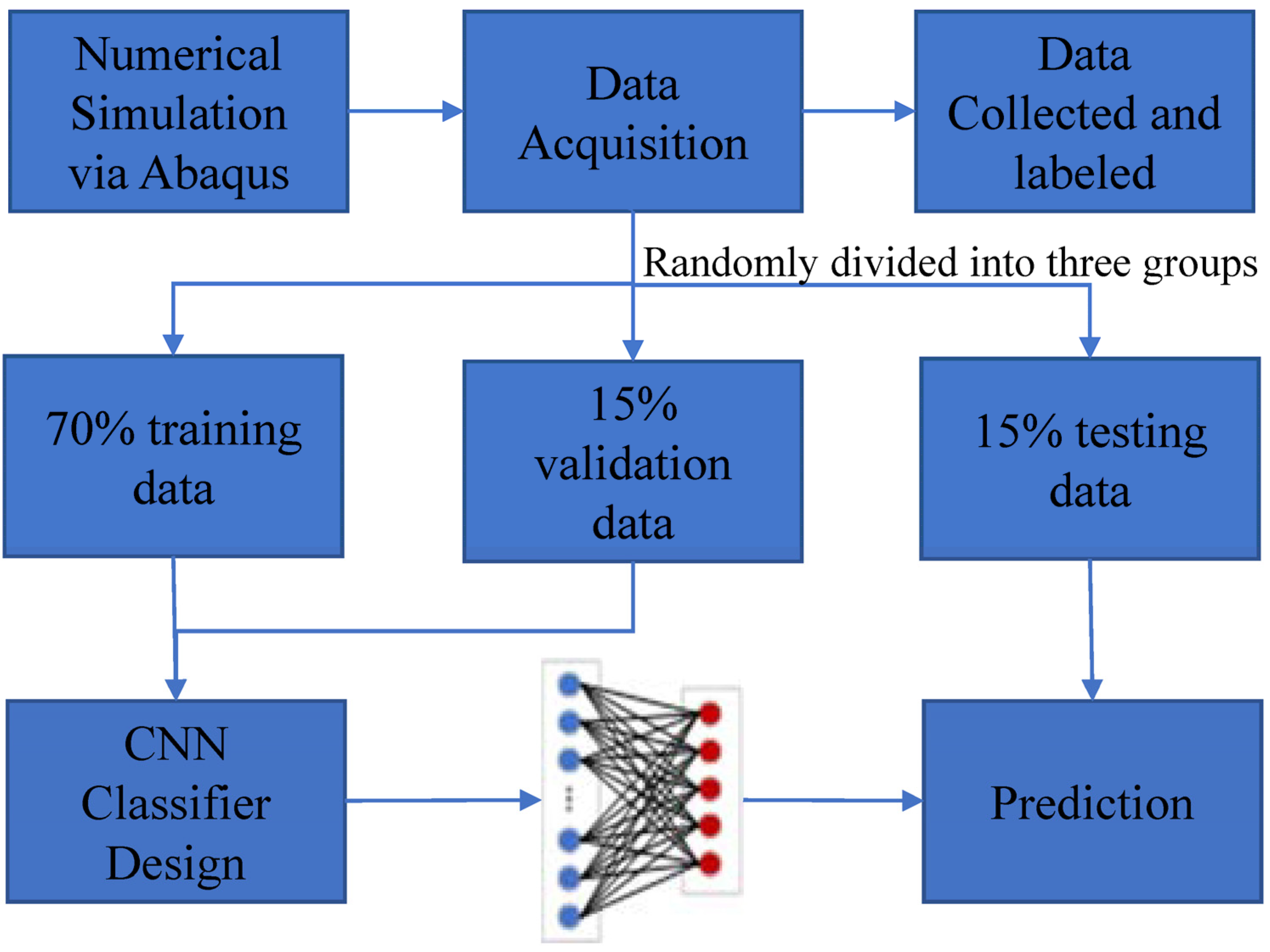
Figure 1. Flow chart of the intended CNN damage detection model.
Ai 05 00075 g001
Figure 2. Process of the convolution layer.
Ai 05 00075 g002
Figure 3. Different activation functions used in training.
Ai 05 00075 g003
Figure 4. The architecture of GoogLeNet.
Ai 05 00075 g004
Figure 5. Example of GASF. (a) Raw vibration obtained in ABAQUS model; (b) image obtained by GASF.
Ai 05 00075 g005
Figure 6. Modeling of the truss in ABAQUS.
Ai 05 00075 g006
Figure 7. The MP2 time history of one damage case on the truss in ABAQUS.
Ai 05 00075 g007
Figure 8. The process of the proposed damage evaluation method using images of vibration and raw images of defects.
Ai 05 00075 g008
Figure 9. Images obtained by GASF.
Ai 05 00075 g009
Figure 10. Paired image of the truss and vibration images obtained by GASF.
Ai 05 00075 g010
Figure 11. (a) The accuracy of the training model; (b) the loss of the training model.
Ai 05 00075 g011
Figure 12. The confusion matrix using images of combined optical truss photos and vibration data image.
Ai 05 00075 g012
Figure 13. The accuracy of the training model at 80 iterations with different numbers of inception layers.
Ai 05 00075 g013
Figure 14. The accuracy of the training model at 80 iterations with different learning rates.
Ai 05 00075 g014
Figure 15. The accuracy of the training model at 80 iterations with different activation functions.
Ai 05 00075 g015
Figure 16. The accuracy of the training model at 80 iterations with different optimizers.
Ai 05 00075 g016
Figure 17. Effect of training data sizes on the accuracy of the GoogLeNet model at different iteration steps.
Ai 05 00075 g017
Table 1. The architecture of the GoogLeNet algorithm.
TypePatch Size StrideOutput SizeDepth
Convolution7 × 7/2112 × 112 × 641
max pool3 × 3/256 × 56 × 640
Convolution3 × 3/156 × 56 × 1922
max pool3 × 3/228 × 28 × 1920
inception (3a)-28 × 28 × 2562
inception (3b)-28 × 28 × 4802
max pool3 × 3/214 × 14 × 4800
inception (4a)-14 × 14 × 5122
inception (4b)-14 × 14 × 5122
inception (4c)-14 × 14 × 5122
inception (4d)-14 × 14 × 5282
inception (4e)-14 × 14 × 8322
max pool3 × 3/27 × 7 × 8320
inception (5a)-7 × 7 × 8322
inception (5b)-7 × 7 × 10242
avg pool7 × 7/11 × 1 × 10240
Dropout (40%)-1 × 1 × 10240
Linear-1 × 1 × 10001
soft max-1 × 1 × 10000
Table 2. Damage positions for different cases.
case12345678910111213141516
span-S1S2S3S4S1S2S1S2S3S4S1S2S3S4S5
face-ffffttfffffffff
element-TTTTmmmmmmrrrrm
Disclaimer/Publisher’s Note: The statements, opinions and data contained in all publications are solely those of the individual author(s) and contributor(s) and not of MDPI and/or the editor(s). MDPI and/or the editor(s) disclaim responsibility for any injury to people or property resulting from any ideas, methods, instructions or products referred to in the content.