Article

Remote Sensing Crop Water Stress Determination Using CNN-ViT Architecture

School of Geomatic Sciences and Surveying Engineering, Agronomic and Veterinary Institute Hassan II, Rabat-Instituts, BP 6202 Madinat Al Irfane, Rabat 10112, Morocco
*
Author to whom correspondence should be addressed.
AI 2024, 5(2), 618-634; https://doi.org/10.3390/ai5020033
Submission received: 25 March 2024 / Revised: 6 May 2024 / Accepted: 7 May 2024 / Published: 9 May 2024
(This article belongs to the Section AI Systems: Theory and Applications)

Abstract

:
Efficiently determining crop water stress is vital for optimising irrigation practices and enhancing agricultural productivity. In this realm, the synergy of deep learning with remote sensing technologies offers a significant opportunity. This study introduces an innovative end-to-end deep learning pipeline for within-field crop water determination. This involves the following: (1) creating an annotated dataset for crop water stress using Landsat 8 imagery, (2) deploying a standalone vision transformer model ViT, and (3) the implementation of a proposed CNN-ViT model. This approach allows for a comparative analysis between the two architectures, ViT and CNN-ViT, in accurately determining crop water stress. The results of our study demonstrate the effectiveness of the CNN-ViT framework compared to the standalone vision transformer model. The CNN-ViT approach exhibits superior performance, highlighting its enhanced accuracy and generalisation capabilities. The findings underscore the significance of an integrated deep learning pipeline combined with remote sensing data in the determination of crop water stress, providing a reliable and scalable tool for real-time monitoring and resource management contributing to sustainable agricultural practices.

1. Introduction

Agriculture is the backbone of our global food supply, a notion underscored by its direct impact on global food security and its significant portion in the global economy [1,2]. The need for efficient management of crop health and water resources has been recognised in multiple studies, highlighting its importance in augmenting agricultural productivity [3,4]. Particularly, the precise determination of crop water stress plays a pivotal role in optimising irrigation practices and enhancing agricultural productivity [5,6]. Traditional methods of assessing water stress often rely on ground-based measurements and manual observations, which are labour-intensive, time-consuming, and limited in their spatial coverage [1,7,8]. As the world’s population continues to grow and climate change poses increasingly unpredictable challenges, the demand for scalable and accurate methods for monitoring crop water stress has never been more pressing.
Recent advancements in deep learning techniques, in conjunction with the wealth of remote sensing data available through satellites, have the potential of opening up promising avenues for automating the assessment of crop water stress [5,7,9]. These technologies offer the potential to provide timely and spatially comprehensive insights into the condition of crops, enabling more effective and sustainable agricultural practices [2,10]. However, leveraging deep learning for this task is not without challenges. Deep learning, although successfully applied in various other fields like image recognition, speech recognition, and natural language processing, still necessitates exploration in the agricultural domain, particularly in the context of crop water stress assessment [11].
One primary challenge is the complex interplay between spectral bands and vegetation indices in satellite imagery, which can be influenced by various environmental factors [12,13,14]. Additionally, defining thresholds for water stress can be quite challenging as they may vary significantly across different crop types [15,16]. The recent literature indicates the underutilisation of satellite imagery compared to digital imagery and UAVs and the prevailing dominance of CNN architectures [5,7]. Existing research in this domain primarily focuses on characterising water stress at the field level, often overlooking the critical variability that can exist within the same field [11,12]. To harness the full potential of deep learning techniques for crop monitoring, there is a pressing need for an end-to-end pipeline designed to provide within-field characterisation, applicable universally across diverse crop types, and scalable to handle the vast amount of available remote sensing data.
While the transformer architecture introduced in the paper “Attention Is All You Need” has become the go-to standard for natural language processing tasks [17], its adaptation to computer vision applications was initially relatively limited [18]. The initial limitation in adapting the transformer architecture to computer vision tasks stemmed from its original design for sequential text data, differing from the spatial, multi-dimensional nature of image data. Traditional convolutional neural networks (CNNs) were favoured due to their locality sensitivity and computational efficiency in handling image data [19,20]. The lack of precedent and the necessary modification efforts to preserve spatial information in transformers further delayed its adaptation to computer vision. However, the landscape of computer vision has evolved, and in particular, vision transformers have garnered substantial attention in recent years. In Ref. [19], the authors present recent vision transformer architectures and their key characteristics. The study emphasises the emerging trend of hybrid vision transformers and their potential to deliver high performance in computer vision applications. They highlight the advantages of hybridisation which have demonstrated remarkable results. The association of the convolution operation and self-attention mechanism has the benefit of exploiting both the local and global image features. The study [20] investigated the application of vision transformers in medical computer vision. The authors reviewed the use of vision transformers’ architectures in many medical areas and discussed the challenges and the future directions for medical research. They also highlighted the contribution of vision transformers in the automatic diagnostics of diseases using medical imagery. Other advancements, such as the deep learning model WetMap [21], exemplify the fusion of convolutional neural networks (CNNs) and vision transformer architectures, leading to remarkable achievements in precise wetland mapping. In their study, a deep learning algorithm was developed, which utilises both CNNs and vision transformer architectures for precise mapping of wetlands. This algorithm has been applied successfully in three pilot sites in Canada. These studies show that vision transformers’ ability to harness the power of attention mechanisms has enabled them to excel at extracting global contextual information in images, a task that CNNs have traditionally struggled with [19,22]. As a result, vision transformers have emerged as a promising alternative in the realm of remote sensing and computer vision [23], prompting us to explore their potential alongside CNNs in the hybrid CNN-ViT architecture for precise crop water stress determination.
In light of these developments, our study proposes the use of a hybrid CNN, h-ViT architecture for crop water stress determination. This architecture is now adopted to address the complexities of agricultural resource monitoring and management, in order to support sustainable agricultural practices. Employing CNN-ViT within this domain presents several challenges: firstly, the need to accurately interpret and utilise the intricate spectral signatures of crops at a fine-grained level, and secondly, the requirement to handle the high variability and heterogeneity inherent in within-field data. Consequently, we designed an end-to-end pipeline to navigate these challenges, encompassing data preprocessing, feature extraction, model training, and final prediction. This comprehensive approach is essential for enhancing the accuracy and efficiency of the process by ensuring that each step is optimally tailored to the specific requirements of within-field crop water stress determination, linking advanced deep learning techniques to practical agricultural applications. Additionally, we conducted a comparative analysis using this hybrid model against a standalone visual transformer architecture, evaluating the effectiveness of the CNN-ViT fusion.
The remaining sections of this paper are organised as follows: Section 2 details the materials and methods employed to achieve our research goals, along with the underlying motivation. Section 3 presents the results and facilitates a comparative evaluation of the two models (ViT and CNN-ViT), which are subsequently discussed in Section 4. Section 5 concludes the paper.

2. Materials and Methods

2.1. Study Area

The current study is centred on Manitoba, a province situated in the heart of Canada (Figure 1). Its approximate geographic coordinates span from 49° to 60° North latitude and 95° to 102° West longitude. It shares borders with the provinces of Saskatchewan to the west, Ontario to the east, Nunavut to the north, and the United States (specifically North Dakota and Minnesota) to the south. The study area encompasses an area of 1248 km2.

2.2. Data

2.2.1. Ground Truth Data

The dataset used is derived from the satellite mission ‘The Soil Moisture Active Passive’ (SMAP), which aims to assess soil moisture levels at each location on Earth [24]. It serves as a validation dataset for the measurements obtained from the satellite.
The observations were conducted using the Passive Active L-band System (PALS), a remote sensing instrument designed to measure soil moisture and vegetation water content. This instrument was mounted on a DC-3 aircraft at an incidence angle of 40°. The aircraft then traversed the experimental area, approximately 27 km × 48 km in the Manitoba region, at an altitude of 3000 m, collecting measurements at intervals of 500 m along a regular grid [24].
The PALS instrument operates in both passive and active modes. In passive mode, it measures the brightness temperature of microwave radiation emitted by the Earth’s surface, which is influenced by soil moisture and vegetation water content. In active mode, the instrument transmits a microwave pulse towards the surface and measures the time it takes for the reflected signal to return. It utilises L-band radiation, which penetrates the soil and vegetation surface to reach the root zone where most of the water is stored. This measurement was employed to calculate soil moisture and vegetation water content.
a
Dataset composition
The measurements were acquired over a period of twelve days, spanning from 8 June to 22 July 2016. We selected the date for which a satellite image covering the same area is available. The data for each date are provided in text format (.txt) and include the coordinates of each measurement point, the crop type, the acquisition date, and the measured variables.
The dataset encompasses a variety of crop types, with soybean being the most prominent, constituting 38% of the dataset. Cereal crops follow closely behind, representing 33%. Colza, though accounting for a smaller proportion at 11.9%, remains a significant component. Maize and oats make up 9.2% and 2.2%, respectively, while other miscellaneous crops collectively contribute 5.7% to the dataset.
b
Measured variables
The dataset includes several variables such as vertically and horizontally polarised brightness temperature, effective soil temperature, and effective vegetation temperature. However, our primary focus was on the volumetric soil moisture content and vegetation water content, as these measurements exhibit greater variability in our dataset.
Volumetric Soil Moisture (VSM) represents the amount of water contained in the soil per unit volume of soil:
  • Expressed as a fraction (m3/m3);
  • Derived from PALS brightness temperature measurements using an algorithm [24];
  • The accuracy of soil moisture measurements was assessed using field-collected and laboratory-determined data. Measurement uncertainties are provided as attributes in the data file.
Vegetation Water Content (VWC) refers to the quantity of water contained within plants:
  • Expressed in kilograms of water per square meter (kg/m2);
  • Estimated from optical satellite observations calibrated with field measurements. For each crop class, a least squares method was employed to establish the relationship (Equation (1)) between the Normalised Difference Vegetation Index (NDVI) and the measured VWC.
VWC = 1.9134   ×   NDVI 2 - 0.3125   ×   NDVI + stem _ factor × NDVI max NDVI min 1 - NDVI min .
where:
-
NDVImax: This parameter refers to the maximum annual NDVI at a given location. Like NDVI, it is closely related to land cover types;
-
NDVImin: This parameter refers to the minimum annual NDVI at a given location;
-
Stem_factor: It is an estimate of the maximum amount of water present in the stems.
Moving forward, VWC is used as it is revealed that variables directly related to crop responses are more representative of the hydric state than soil-related variables [2].

2.2.2. Remote Sensing Data

The thermal band response of vegetation serves as a robust indicator of its water stress levels [25]. This is due to the inverse correlation between plant temperature and water stress, as stressed plants usually exhibit elevated canopy temperatures due to stomatal closure aimed at minimising water loss [26]. Hence, a sensor was chosen that provides thermal information while maintaining a reasonably good spatial resolution.
Landsat 8 is equipped with crucial sensors: the Operational Land Imager (OLI) and the Thermal Infrared Sensor (TIRS). These sensors enable the acquisition of multispectral imagery spanning various spectral bands. Each of these bands corresponds to a specific segment of the electromagnetic spectrum, facilitating the measurement of distinct optical properties related to the reflectance and emissivity of the Earth’s surface. Notably, these bands exhibit different spatial resolutions, ranging from 30 m (for bands covering the visible, near-infrared, and mid-infrared regions) to 100 m (for thermal bands).
A cloud-free Landsat 8 image, acquired on 18 July 2016, was chosen for analysis, representing a Level 2 Science Product (L2SP) in terms of data processing. The decision to utilise this particular satellite image for the study area was primarily based on two pivotal criteria: the absence of cloud cover and the availability of corresponding ground truth data.
The bands used in this study are listed in Table 1.

2.3. Methodology

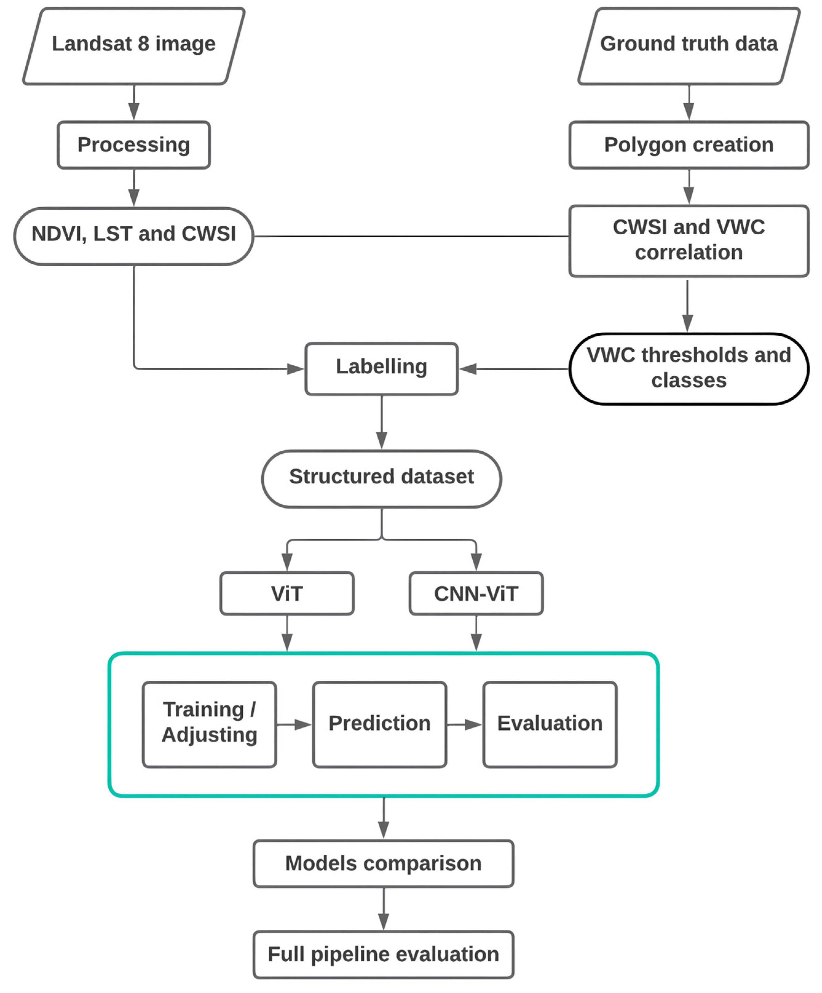
Our research is dedicated to establishing a detailed, end-to-end methodology for accurately determining crop water stress. This methodology spans the entire spectrum from the initial data selection to the final analysis phase (Figure 2). The proposed methodology consists of several key stages: (1) Initial data preprocessing, involving extensive preparation and annotation of data, management of spectral bands and indices, and precise determination of class thresholds; (2) The deployment and assessment of a standalone vision transformer model; (3) The subsequent adaptation and application of the CNN-ViT architecture for refined crop water status determination. Following these steps, we conducted a comparative analysis to evaluate the efficacy of the vision transformer and CNN-ViT architectures in identifying crop water stress, accompanied by an extensive Discussion.

2.3.1. Data Processing

a
Ground truth data processing
The total number of points measured per acquisition date was 5184. However, there were certain measurements associated with classes other than vegetation. The data file contains a ‘Land Cover’ attribute (LC). Using ArcGIS 10.8 software, we displayed the points based on their coordinates, utilising the NAD83/UTM Zone 14N coordinate system. To optimise pixel labelling while considering the point nature of our data, we implemented an approach involving the creation of square buffers with sides measuring 240 m around each point. This strategy aimed to increase the accurately labelled pixel count without altering intra-parcel characterisation. Subsequently, we selectively removed polygons for which the land cover did not correspond to vegetation. As a result, the final number of labelled polygons corresponding to vegetation areas was 4357.
b
Remote sensing data processing
The acquired remote sensing data underwent several critical processing steps to ensure its quality and suitability for analysis. Cloud and shadow masking techniques were applied to identify and remove pixels affected by clouds, haze, or shadows. Unwanted pixels were marked as “NoData” to maintain data integrity. Additionally, data normalisation was performed to standardise the dimensions of the input data, facilitating model training and enhancing its stability and generalisation.
c
NDVI and LST calculation
The performance of deep learning models relies on their ability to process large volumes of data to extract relevant information and model spatial relationships. With this in mind, we chose to include not only the imagery bands but also the Normalised Difference Vegetation Index (NDVI) and Land Surface Temperature (LST) in the model input. The addition of NDVI enables the capture of information regarding vegetation density and its condition, which is crucial for crop analysis and water stress detection. LST, on the other hand, provides insights into Earth’s surface temperature, aiding in the understanding of thermal variations related to soil moisture and water stress. By incorporating these additional variables, we enhanced the model’s input data with vegetation-specific and temperature-related information, potentially improving the model’s capacity to characterise and predict crop water stress more accurately.
Healthy vegetation exhibits a highly characteristic spectral reflectance curve with a strong response in the near-infrared band and a relatively weaker response in the red band. The Normalised Difference Vegetation Index (NDVI) quantifies this difference as a numerical value ranging from −1 to 1.
NDVI is computed using Landsat 8’s Band 4 (Red) and Band 5 (Near Infrared, NIR) following Equation (2).
NDVI = NIR Red NIR + Red
Land surface temperature can be computed using Landsat 8’s thermal band, following the formula recommended by the United States Geological Survey [27]. This calculation involves several steps outlined in Figure 3. Specifically, the input for the calculation includes three bands from Landsat 8, which are Band 4 (red wavelength; 0.64–0.67 μm), Band 5 (near infrared (NIR) wavelength; 0.85–0.88 μm), and Band 10 (thermal infrared sensor (TIRS) wavelength; 10.60–11.19 μm).
d
Crop water stress classes
Deep learning models are employed to predict a pixel’s affiliation with a specific class. To apply this approach to our variable VWC (Vegetation Water Content), it is necessary to categorise our value range into meaningful crop water stress classes. According to the findings from our literature review, utilising three distinct classes (low water stress, moderate water stress, and high water stress) is a relevant approach, as there has been an observed negative correlation between model performance and the number of classes employed [7,12]. It is worth noting that the selection of classification thresholds depends on various factors such as specific crop type, growth stage, environmental conditions, and irrigation practices [2,28]. Given that the thresholds for the Crop Water Stress Index (CWSI) are known and can be generalised, we attempted to establish a correlation between CWSI and our VWC variable to determine suitable thresholds for our classification [29].
  • CWSI calculation
We employed an approach solely based on the thermal band of the Landsat 8 satellite, as proposed and validated by Ref. [30].
It is important to note that a CWSI value close to 1 indicates a high presence of water stress, while a value near 0 indicates the absence of water stress.
CWSI   = T S T Cold T Hot T Cold
where
-
TS: Land surface temperature, LST.
-
TCold: Temperature of the ‘coldest’ vegetated pixel.
-
THot: Temperature of the ‘hottest’ vegetated pixel.
The selection of the ‘coldest’ vegetated pixel was achieved by applying an NDVI threshold greater than 0.5. Among the pixels meeting this criterion, we selected the 10% with the coldest temperatures and, then, chose the pixel with the lowest value among them. Similarly, the selection of the ‘hottest’ vegetated pixel was performed by applying an NDVI threshold greater than 0.2.
  • Correlation between CWSI and VWC
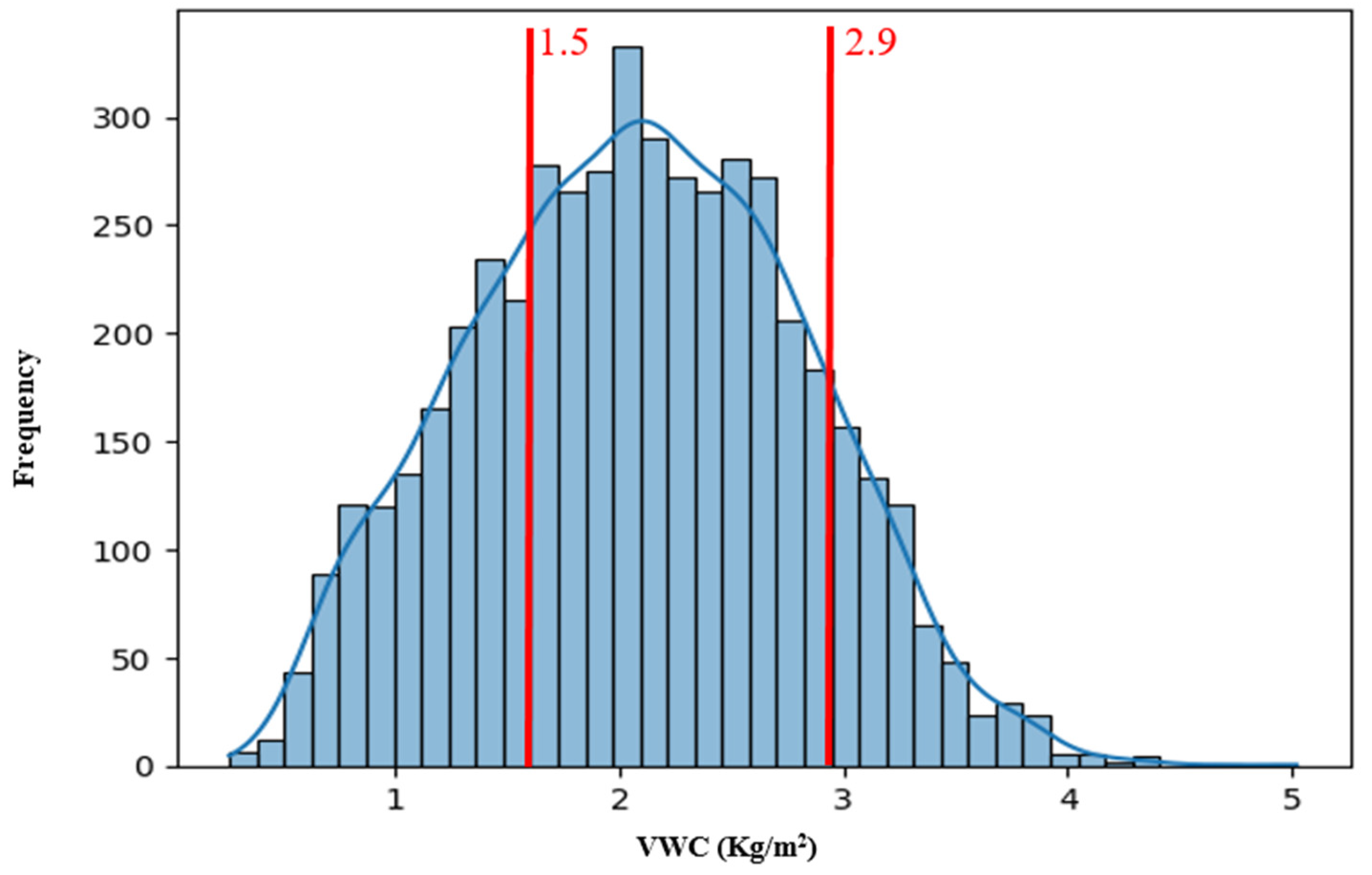
By having data for which both CWSI and VWC values are known, we can establish the correlation between these two variables and translate known CWSI thresholds into thresholds for our VWC variable.
Within the ArcGIS software, we extracted CWSI values for points with known VWC values. Subsequently, we performed a data linkage between these datasets and conducted a correlation analysis. The results revealed a significant inverse correlation with a correlation coefficient of r = −0.63. The significance of this correlation is underscored by the correlation coefficient being significantly different from zero with a significance level of 0.05. This signifies a noteworthy association between CWSI and VWC, where a reduction in VWC corresponds to an elevation in CWSI, indicating the presence of water stress.
  • CWSI thresholds
According to [30,31], generalised CWSI thresholds are presented in the following table. Based on these values, corresponding VWC thresholds were determined as follows (Table 2).
For CWSI, values exceeding 0.8 typically do not correspond to vegetation.
Figure 4 illustrates the distribution of VWC values along with the thresholds adopted for the creation of the three classes.
e
Dataset labelling
The labelling process followed a structured sequence of steps. Initially, polygons denoting VWC measurement positions were categorised into the predefined classes as discussed earlier. Subsequently, these categorised polygons underwent a transformation into a raster representation. Within this raster representation, each pixel was assigned a value of 1, 2, or 3, in accordance with its corresponding class.
The outcome of the labelling process was exported in TIFF format, matching the dimensions of the satellite image (1542 × 917 pixels). In this format, any unannotated area is designated as the background (class 0).
The dataset was divided into training (60%), validation (10%), and test (30%) sets, ensuring balanced distribution through random shuffling. The final evaluation was conducted on the independent test set, which was reserved solely for assessing the model’s performance on unseen data.

2.3.2. Visual Transformers

Visual transformers depart from traditional convolutional neural networks by treating images as sequences of fixed-size, non-overlapping patches. These patches undergo a two-step transformation: first, they are linearly embedded into high-dimensional vectors, and second, a positional embedding is added to encode the spatial location of each patch. The resulting embedding are then processed through a stack of self-attention layers, reminiscent of the transformer model initially developed for natural language processing tasks.
The series of self-attention layers within visual transformers are instrumental in enabling the model to capture contextual relationships between patches. This occurs both at a local scale, where patches attend to their neighbouring patches, and at a global scale, where long-range dependencies across the entire image are recognised. This ability to assign attention weights to other patches based on their content allows visual transformers to understand complex relationships and contextual information within images, ultimately contributing to its outstanding performance in various computer vision benchmarks.

2.3.3. CNN-ViT

The proposed model is a resource-efficient CNN-ViT architecture that incorporates local window attention mechanism (LWA) to make effective use of the spectral signatures of crops. To better align with the study input data and use case, we made structural and hyperparameter changes. The proposed network comprises three critical components: a feature extraction block, a deep multi-scale convolution block, and a visual transformer with local window attention [21]. The proposed architecture is depicted in Figure 5, where the ⨁ symbol represents element-wise addition. Xpatch represents the model’s input, and O corresponds to the prediction. Details of the model are depicted in Table 3.
The initial step involves creating training patches with dimensions of 8 × 8 × 8. Each patch is generated by traversing each input band and defining a region centred around each pixel. We added padding around the images to ensure that patches near the image borders also have sufficient context.
Simultaneously, as we created input patches, we also generated corresponding patches for the labels. This ensured that each training patch was associated with the appropriate label. In the context of this process, we specifically excluded patches related to the background, focusing solely on the classes of interest.
Feature Extractor Block: The feature extractor block employs both 3D and 2D convolutions, along with parallel branches, to extract both spatial and spectral features. This intricate architecture enables the capture of rich information while maintaining computational efficiency.
Initially, the input data of size 8 × 8 × 8 is reshaped into 8 × 8 × 8 × 1 to align with the convolutional layer requirements. Subsequently, two 3D convolutional layers are applied, utilising 16 and 32 filters with kernel sizes of 1 × 1 × 3 and 1 × 1 × 5, respectively. These convolutions enable the capture of both spatial and spectral information.
The results are then directed to two parallel branches, F1 and F2. Branch F1 comprises a convolutional encoder and decoder. The encoder consists of two separable 2D convolution layers with 32 filters and a kernel size of 3 × 3. The decoder consists of two 2D transposed convolution layers followed by a 2D up-sampling layer, facilitating the extraction and reconstruction of spatial features. Branch F2, on the other hand, employs a 2D convolution with 32 filters, a stride of 2, and a kernel size of 3 × 3. This convolution captures additional information and combines it with the features extracted from branch F1.
Finally, the results from both branches are summed to obtain a final feature map with dimensions 8 × 8 × 32.
This architecture effectively combines spatial and spectral information while maintaining reasonable computational complexity [21]. Figure 6 and Table 4 depict the feature extractor block architecture.
Depth-Wise Convolution Block: To mitigate potential overfitting due to a large number of parameters, three parallel depth convolutions are employed. Each depth convolution uses a 64-sized filter and different kernel sizes (1 × 1, 3 × 3, and 5 × 5), respectively. Features from the feature extractor network, with a size of 8 × 8 × 32, serve as input data for the depth convolution block.
Local Attention Window: By integrating LWA into the semantic segmentation architecture, the model can focus on creating local neighbourhood areas around each query element. This allows the model to capture fine local details and relationships between neighbouring pixels. LWA enhances the model’s ability to concentrate on relevant information in the local region while disregarding irrelevant or distracting details.

2.3.4. Implementation Details

Implementing deep learning models can be computationally intensive, often necessitating GPU resources. We leveraged open-source tools, including Google Colaboratory for cloud-based computation like free access to GPU resources like Tesla T4 and 13 GB RAM, TensorFlow for its extensive capabilities, and Keras as a user-friendly neural network API, streamlining model development and deployment.
a
Hyperparameter optimisation
Training functions: The models in our study were not based on pre-trained architectures and utilised distinct methods for weight initialisation. Both the visual transformer and CNN-ViT models were initialised using the “Glorot uniform” method.
For multi-class problems like our study, the “sparse categorical cross-entropy”, a variation of “categorical cross-entropy”, is frequently used as the loss function. It is suitable when labels are represented as integers (rather than one-hot vectors, as in standard categorical cross-entropy). This loss function is particularly appropriate when predicting mutually exclusive classes, where a data example can belong to only one class. We used this loss function along with the ‘softmax’ activation function for classification in both architectures. For convolutional layers, we employed the ReLU (Rectified Linear Unit) activation, while the GELU (Gaussian Error Linear Unit), commonly used in transformer-based architectures, was employed for CNN-ViT components.
The optimisation algorithm employed in this study was AdamW, a variant of the Adam algorithm that incorporates weight decay. The Adam algorithm is known for its ability to adapt learning rates adaptively for each model parameter, making it efficient for rapid convergence and handling gradients of different scales. This enhancement applies a penalty to the model’s weights during gradient updates. This weight penalty reduces their magnitude, which can help prevent overfitting by favouring smaller weights.
Hyperparameters: To tune hyperparameters of the adopted models, we employed an iterative strategy to mitigate the time- and resource-intensive nature of techniques like random and grid search. This iterative method initially defines a range of possible values for each hyperparameter, followed by multiple training and evaluation cycles with different hyperparameter combinations. At each iteration, model performance is assessed on a validation set, and hyperparameter values are adjusted accordingly. This iterative approach enables us to glean insights from the model’s performance at each step, progressively refining hyperparameters for improved results.
Learning rate: The default Adam optimiser rate of 0.001 was incrementally adjusted. The visual transformer and CNN-ViT benefited from an increased rate of 0.01 for faster convergence without raising instability concerns.
Batch size: We compared various options. The visual transformer and CNN-ViT were evaluated on batch sizes of 64, 128, and 256 elements, with 256 being the optimal choice alongside their specific learning rates.
Epochs: Both models were initially set to 500 epochs. However, we implemented early stopping mechanisms to limit epochs to 100 for visual transformer and CNN-ViT. This strategy prevents potential model performance deterioration while ensuring efficient training.
b
Regularisation techniques
Regularisation is used to combat overfitting, which occurs when the classification error on the validation dataset is higher than that on the training dataset. It is one of the most common issues when applying learning techniques, especially for models with a large number of parameters. In this work, the following regularisation techniques were implemented: Dropout, data augmentation, weight decay, and early stopping.
Dropout: a regularisation technique that involves randomly deactivating a portion of neurons and their connections during the training of a neural network. Each neuron in the network has a probability of P% of being active and a probability of (1 − P) % of being deactivated. The value of the probability P is a hyperparameter that needs to be adjusted. At the end of the experiments, a dropout rate of 0.4 was deemed sufficient for the visual transformer and the hybrid model.
Data augmentation: To enhance the models’ performances, we augmented the training data artificially by applying the following transformations:
  • Random horizontal flipping;
  • Random rotation of images with a rotation factor of 0.02 radians;
  • Random zooming of images by adjusting their height and width with a factor of 0.2.
By introducing these transformations, the training data becomes more diverse, enabling the models to learn from a broader range of scenarios and patterns. Consequently, the models exhibit improved generalisation and perform better when making predictions on new data.
Weight decay: A weight decay of 0.0001 was applied. This means that a small penalty was added to the loss function when updating the model’s weights. This penalty encourages the weights to have smaller values, which limits the model’s complexity and helps regulate learning.
Early stopping: During training, early stopping monitors the model’s performance on the validation set and records the weights corresponding to the best performance. At each training iteration, if the performance on the validation set improves, the model’s weights are saved. When the performance on the validation set starts to deteriorate, training is stopped prematurely, and the weights associated with the best performance are retrieved. These weights correspond to the point where the model had the best generalisation ability.
By retaining the weights corresponding to the best performance on the validation set, early stopping helps select the optimal model for prediction on new data.
c
Evaluation metrics
The performance of each model was quantitatively assessed using five performance metrics: accuracy, recall, precision, F1 score, and Cohen’s Kappa. Accuracy measures the percentage of predicted values that match actual values for each model. Recall is defined as the ratio of the number of true positives to the sum of true positives and false negatives, and precision is the ratio of the number of true positives to the sum of true positives and false positives for each model. The F1 score represents the harmonic mean of recall and precision, and Cohen’s Kappa assesses the agreement between predicted and actual values, considering chance agreement, for each individual model.

3. Results

3.1. Visual Transformer

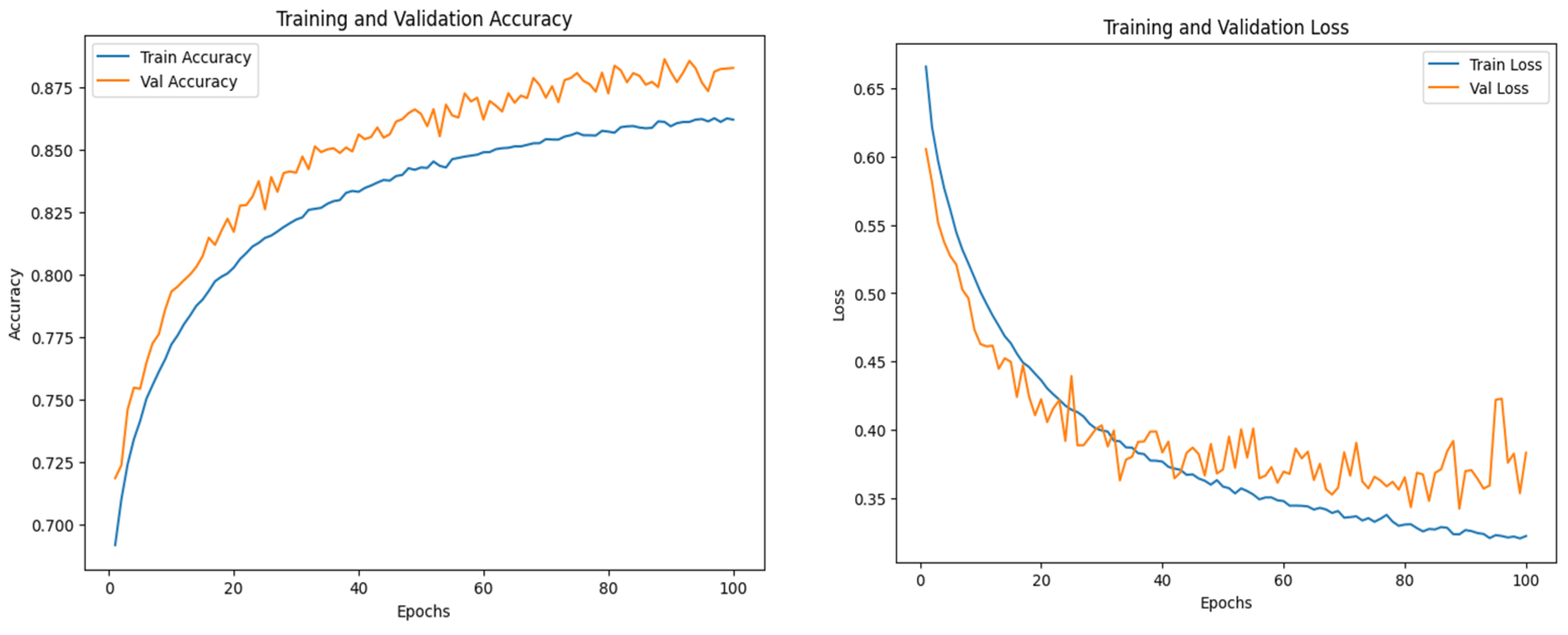
The training duration for this model was 54 min. The model starts showing considerable diversion after the 100th epoch. Even if the model’s accuracy is higher than the training one, the validation loss does not converge (Figure 7).
The validation set plays a crucial role in hyperparameter tuning, enabling the adjustment of model parameters to mitigate overfitting. Performance metrics such as precision, recall, F1 score, and the kappa coefficient were calculated for each class. To ensure a balanced evaluation independent of class size or distribution, macro averaging was employed.
The vision transformer ViT model demonstrates strong overall accuracy on both validation and test datasets, with values around 88%, indicating its ability to correctly classify pixels into their respective semantic classes. Cohen’s Kappa score is notably high, indicating a substantial level of agreement between the model’s predictions and ground truth labels. Furthermore, the F1 score of 85% demonstrates the model’s ability to effectively capture both false positives and false negatives (Table 5).

3.2. CNN-ViT

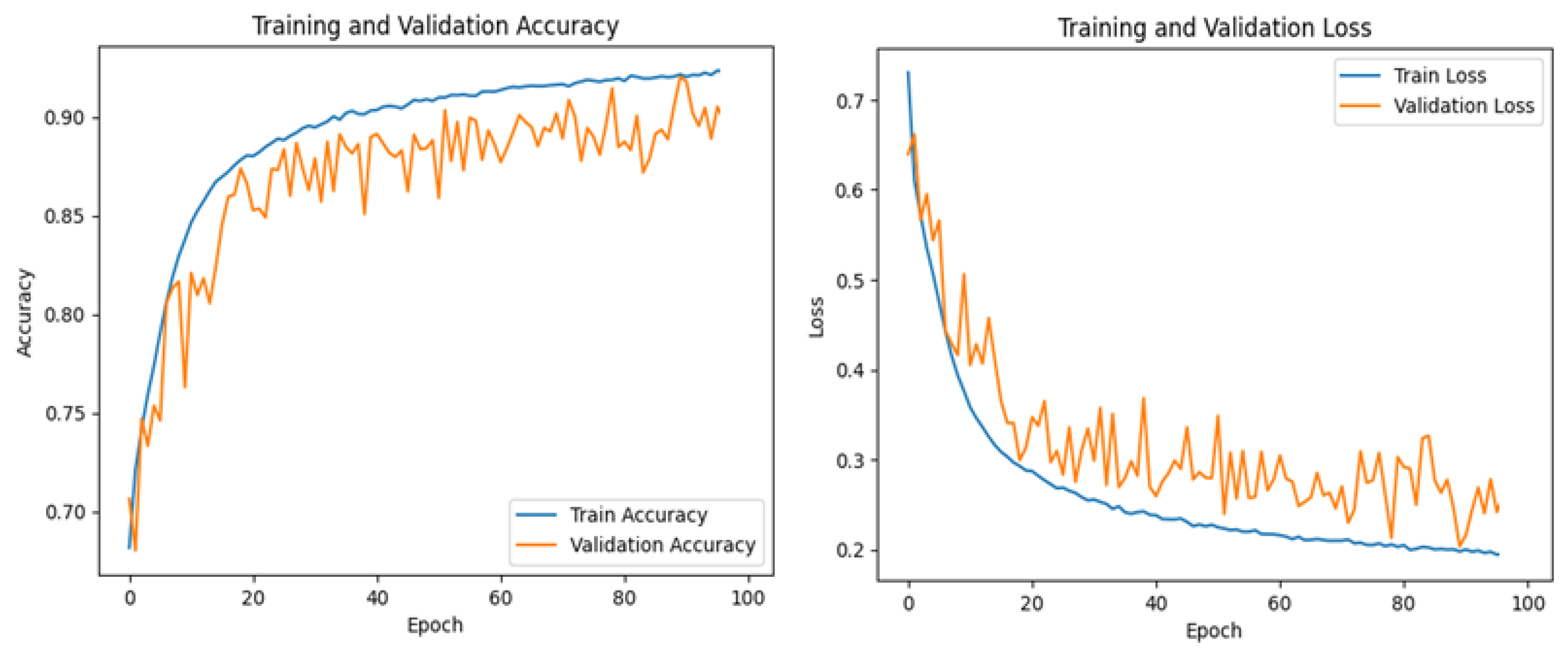
The training time for this model was 1 h and 2 min. The model starts to show global stability around the 100th epoch. During training, the model exhibits minor local instability, characterised by oscillations in precision and loss, which persist despite efforts to address them, including a reduced learning rate of 0.001 and the application of various regularisation techniques (Figure 8).
The model achieves a high overall accuracy, indicating correct predictions in approximately 90.4% of cases. Kappa score is high (82%), indicating an excellent level of the model’s prediction agreement compared to actual values. The F1 score is 88%, which demonstrates the model’s ability to effectively capture both false positives and false negatives.
When assessing the CNN-ViT model’s performance on the test dataset, the results align closely with those from the validation set, indicating its robust generalisation capabilities (Table 5). In summary, despite the observed local instability, the CNN-ViT model demonstrates global stability, high precision, and effective generalisation when faced with new data.
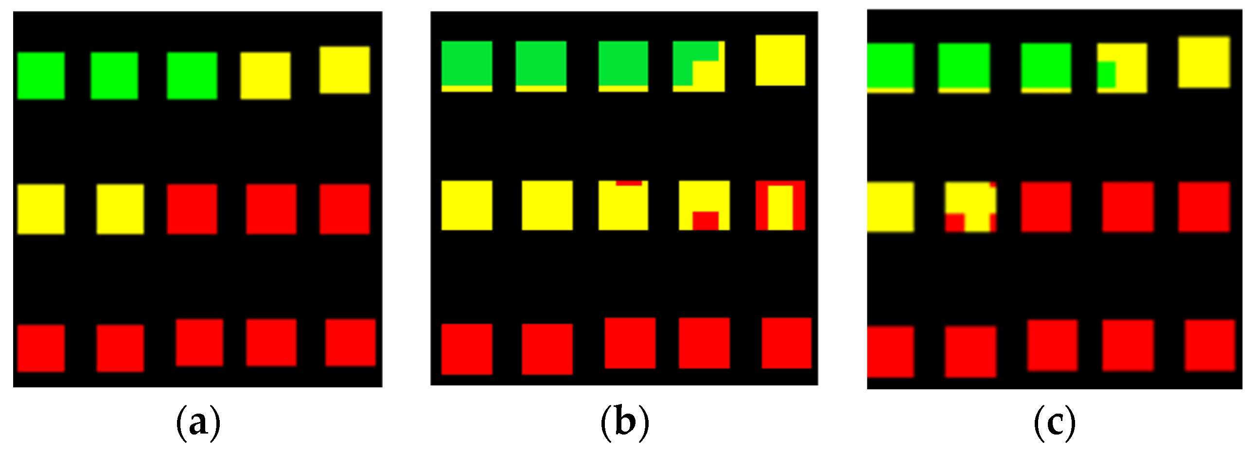
Another approach to assess a model’s performance is to visualise its prediction results. From a visual standpoint, CNN-ViT’s results closely resemble the ground truth data (Figure 9).
In our implementation, the visual transformers’ architectures, which focus on patch-based processing, showed a remarkable ability to disregard background pixels and utilise relevant information for accurate learning and prediction. This characteristic was particularly evident in the face of class imbalances. Moreover, they maintained consistent performance with new data sets. The CNN-ViT model demonstrated enhanced results compared to the visual-transformer-only model.
While the CNN-ViT model performed well, it showed a tendency to classify a notable number of elements into the ‘moderate stress’ category, likely due to the prevalence of this class in the training data. To address this, further refinement of the model could involve subdividing the ‘moderate stress’ class into subclasses representing different stress levels. This adjustment could allow the CNN-ViT model to achieve more nuanced differentiation, potentially improving its accuracy and specificity in classifying crop water stress levels.

4. Discussion

This study presents a scientific contribution in utilising deep learning for characterising crop water stress from satellite imagery. Our primary goal was to develop an end-to-end workflow, filling the gap in annotated data and specialised architectures commonly seen in other deep learning applications. This objective was achieved by compiling a dataset from ‘The Soil Moisture Active Passive’ mission and Landsat 8 imagery. This step was critical in our innovative approach, particularly in adapting and applying the CNN-ViT architecture, traditionally used in object detection tasks and some other applications such as wetland mapping, to a more detailed classification task in agriculture for crop water stress determination.
One challenge we faced related to the dependency on datasets specific to certain dates, compounded by the temporal resolution limitations of Landsat 8. This issue made obtaining consistent imagery challenging and raised questions about the precision of intra-field crop water stress determination, especially when enhancing the dataset size by subdividing each pixel.
In transforming Volumetric Water Content (VWC) data into class probabilities, careful consideration was required for the interpretation of these values, as well as the determination of the number and thresholds of classes. Opting for a three-class system, influenced by the literature on model accuracy correlations, we noted a skew in model predictions due to the predominance of the moderate stress class in our dataset. This observation suggested a potential refinement of the class system to improve model performance.
In this study, our exploration of architectures led us to focus on the ViT and the CNN-ViT architectures. These two architectures are based on attention mechanisms that allow (1) focusing on the most informative parts of the satellite image and (2) capturing the complex interdependencies between different regions in the satellite image for a better contextual understanding. These two aspects are crucial to improve the efficiency and accuracy of crop water stress predictions.
The visual transformer architecture achieved a global accuracy of 88% and demonstrated a strong ability to manage class imbalance issues. However, it was the CNN-ViT architecture that showcased exceptional capabilities, efficiently focusing on relevant data while disregarding non-essential elements. This model achieved an overall accuracy superior to 90% and demonstrated stability, a high level of prediction, and effective generalisation with new data. This performance highlighted a new direction in the application of CNN-ViT in precision agriculture for crop water stress determination using remote sensing images, particularly in its adaptability and effectiveness in detailed classification.
This study also encountered instances of local instability, potentially stemming from data noise or model initialisation. A prospective solution might involve initialising model training with a simpler task, like vegetation detection, to establish a baseline of stability before progressing to more complex tasks such as water stress characterisation.
A limitation of our research was the necessity to conduct evaluations within a single area and date, owing to dataset constraints. Ideally, testing under a more diverse set of conditions would offer a stronger validation for our models, providing a more comprehensive understanding of their applicability and robustness in different agricultural settings.

5. Conclusions

This research constitutes an exploratory step into the precise evaluation of crop water stress leveraging deep learning methodologies applied to Landsat 8 satellite data. Central to our approach was the formulation of an end-to-end workflow, initiated with the compilation of an annotated dataset. This foundational phase was essential for the subsequent analytical focus on a visual transformer architecture and, notably, the deployment of the CNN-ViT architecture. The introduction of the CNN-ViT model, integrating Convolutional Neural Networks with Visual Transformers, represented a novel application in the context of crop water stress analysis.
Our analysis indicated that models combining transformer elements with CNNs exhibited enhanced performance capabilities. Specifically, the CNN-ViT model demonstrated remarkable efficacy in delineating localised water stress variations, indicating its substantial utility in detailed agricultural classification scenarios. This implementation of the CNN-ViT model marks a significant advancement in its application spectrum, demonstrating its potential in intricate classification tasks within agricultural contexts.
In summary, this study successfully established a full-stack pipeline for the accurate determination of crop water stress and concurrently highlighted the efficacy of the CNN-ViT architecture in this emerging domain. The integration of visual transformer models with CNN frameworks merits additional research and consideration within the agricultural technology sector.

Author Contributions

Conceptualization, K.L., C.S., M.B. and R.Y.; Methodology, K.L., C.S., M.B. and R.Y.; Validation, K.L., C.S., M.B. and R.Y.; Formal analysis, K.L., C.S., M.B. and R.Y.; Investigation, K.L., C.S., M.B. and R.Y; Resources, M.B. and R.Y.; Writing—original draft preparation, K.L., C.S., M.B. and R.Y.; Writing—review and editing, K.L., C.S., M.B. and R.Y.; Supervision, M.B. and R.Y.; Project administration, M.B.; Funding acquisition, M.B. All authors have read and agreed to the published version of the manuscript.

Funding

This work was supported by the Ministry of Higher Education, Scientific Research and Innovation (Morocco), the Digital Development Agency of Morocco (DDA) and the National Center for Scientific and Technical Research of Morocco (CNRST) (Alkhawarizmi/2020/17).

Institutional Review Board Statement

Not applicable.

Informed Consent Statement

Not applicable.

Data Availability Statement

The dataset used in this article is derived from the satellite mission ‘The Soil Moisture Active Passive’ (SMAP). Available online: https://doi.org/10.5067/WM5FXV7WPQ6F (accessed on 28 July 2023).

Conflicts of Interest

The authors declare no conflicts of interest.

References

  1. Katimbo, A.; Rudnick, D.R.; DeJonge, K.C.; Lo, T.H.; Qiao, X.; Franz, T.E.; Nakabuye, H.N.; Duan, J. Crop water stress index computation approaches and their sensitivity to soil water dynamics. Agric. Water Manag. 2022, 266, 107575. [Google Scholar] [CrossRef]
  2. Virnodkar, S.S.; Pachghare, V.K.; Patil, V.C.; Jha, S.K. Remote sensing and machine learning for crop water stress determination in various crops: A critical review. Precis. Agric. 2020, 21, 1121–1155. [Google Scholar] [CrossRef]
  3. Dutta, S.K.; Laing, A.M.; Kumar, S.; Gathala, M.K.; Singh, A.K.; Gaydon, D.; Poulton, P. Improved water management practices improve cropping system profitability and smallholder farmers’ incomes. Agric. Water Manag. 2020, 242, 106411. [Google Scholar] [CrossRef]
  4. Martinho, V.J.P.D. Efficient water management: An analysis for the agricultural sector. Water Policy 2020, 22, 396–416. [Google Scholar] [CrossRef]
  5. Altalak, M.; Uddin, M.A.; Alajmi, A.; Rizg, A. Smart Agriculture Applications Using Deep Learning Technologies: A Survey. Appl. Sci. 2022, 12, 5919. [Google Scholar] [CrossRef]
  6. Safdar, M.; Shahid, M.A.; Sarwar, A.; Rasul, F.; Majeed, M.D.; Sabir, R.M. Crop Water Stress Detection Using Remote Sensing Techniques. Environ. Sci. Proc. 2023, 25, 20. [Google Scholar] [CrossRef]
  7. Chandel, N.S.; Chakraborty, S.K.; Rajwade, Y.A.; Dubey, K.; Tiwari, M.K.; Jat, D. Identifying crop water stress using deep learning models. Neural Comput. Appl. 2021, 33, 5353–5367. [Google Scholar] [CrossRef]
  8. Ihuoma, S.O.; Madramootoo, C.A. Recent advances in crop water stress detection. Comput. Electron. Agric. 2017, 141, 267–275. [Google Scholar] [CrossRef]
  9. Kamarudin, M.H.; Ismail, Z.H.; Saidi, N.B. Deep Learning Sensor Fusion in Plant Water Stress Assessment: A Comprehensive Review. Appl. Sci. 2021, 11, 1403. [Google Scholar] [CrossRef]
  10. Wang, D.; Cao, W.; Zhang, F.; Li, Z.; Xu, S.; Wu, X. A Review of Deep Learning in Multiscale Agricultural Sensing. Remote. Sens. 2022, 14, 559. [Google Scholar] [CrossRef]
  11. Alibabaei, K.; Gaspar, P.D.; Lima, T.M.; Campos, R.M.; Girão, I.; Monteiro, J.; Lopes, C.M. A Review of the Challenges of Using Deep Learning Algorithms to Support Decision-Making in Agricultural Activities. Remote. Sens. 2022, 14, 638. [Google Scholar] [CrossRef]
  12. Virnodkar, S.S.; Pachghare, V.K.; Patil, V.C.; Jha, S.K. DenseResUNet: An Architecture to Assess Water-Stressed Sugarcane Crops from Sentinel-2 Satellite Imagery. Trait. Signal 2021, 38, 1131–1139. [Google Scholar] [CrossRef]
  13. Polivova, M.; Brook, A. Detailed Investigation of Spectral Vegetation Indices for Fine Field-Scale Phenotyping. In Vegetation Index and Dynamics; Carmona, E.C., Ortiz, A.C., Canas, R.Q., Musarella, C.M., Eds.; IntechOpen: London, UK, 2022. [Google Scholar] [CrossRef]
  14. Duarte-Carvajalino, J.M.; Silva-Arero, E.A.; Góez-Vinasco, G.A.; Torres-Delgado, L.M.; Ocampo-Paez, O.D.; Castaño-Marín, A.M. Estimation of Water Stress in Potato Plants Using Hyperspectral Imagery and Machine Learning Algorithms. Horticulturae 2021, 7, 176. [Google Scholar] [CrossRef]
  15. Fu, Z.; Ciais, P.; Feldman, A.F.; Gentine, P.; Makowski, D.; Prentice, I.C.; Stoy, P.C.; Bastos, A.; Wigneron, J.-P. Critical soil moisture thresholds of plant water stress in terrestrial ecosystems. Sci. Adv. 2022, 8, eabq7827. [Google Scholar] [CrossRef] [PubMed]
  16. Qin, A.; Ning, D.; Liu, Z.; Li, S.; Zhao, B.; Duan, A. Determining Threshold Values for a Crop Water Stress Index-Based Center Pivot Irrigation with Optimum Grain Yield. Agriculture 2021, 11, 958. [Google Scholar] [CrossRef]
  17. Dosovitskiy, A.; Beyer, L.; Kolesnikov, A.; Weissenborn, D.; Zhai, X.; Unterthiner, T.; Dehghani, M.; Minderer, M.; Heigold, G.; Gelly, S.; et al. An Image is Worth 16×16 Words: Transformers for Image Recognition at Scale. arXiv 2021, arXiv:2010.11929. Available online: http://arxiv.org/abs/2010.11929 (accessed on 25 September 2023).
  18. Fu, Z. Vision Transformer: Vit and Its Derivatives. arXiv 2022, arXiv:2205.11239. Available online: http://arxiv.org/abs/2205.11239 (accessed on 15 October 2023).
  19. Khan, A.; Rauf, Z.; Sohail, A.; Khan, A.R.; Asif, H.; Asif, A.; Farooq, U. A survey of the vision transformers and their CNN-transformer based variants. Artif. Intell. Rev. 2023, 56 (Suppl. 3), 2917–2970. [Google Scholar] [CrossRef]
  20. Parvaiz, A.; Khalid, M.A.; Zafar, R.; Ameer, H.; Ali, M.; Fraz, M.M. Vision Transformers in medical computer vision—A contemplative retrospection. Eng. Appl. Artif. Intell. 2023, 122, 106126. [Google Scholar] [CrossRef]
  21. Jamali, A.; Roy, S.K.; Ghamisi, P. WetMapFormer: A unified deep CNN and vision transformer for complex wetland mapping. Int. J. Appl. Earth Obs. Geoinf. 2023, 120, 103333. [Google Scholar] [CrossRef]
  22. Maurício, J.; Domingues, I.; Bernardino, J. Comparing Vision Transformers and Convolutional Neural Networks for Image Classification: A Literature Review. Appl. Sci. 2023, 13, 5521. [Google Scholar] [CrossRef]
  23. Ulhaq, A.; Akhtar, N.; Pogrebna, G.; Mian, A. Vision Transformers for Action Recognition: A Survey. arXiv 2022, arXiv:2209.05700. Available online: http://arxiv.org/abs/2209.05700 (accessed on 13 October 2023).
  24. Colliander, A.; Misra, S.; Cosh, M. SMAPVEX16 Manitoba PALS Brightness Temperature and Soil Moisture Data, Version 1’ [VSM_20160718, VWC_20160718]. Boulder, Colorado USA. NASA National Snow and Ice Data Center Distributed Active Archive Center, 2019. Available online: https://nsidc.org/data/sv16m_pltbsm/versions/1 (accessed on 28 July 2023).
  25. Zhou, Z.; Majeed, Y.; Naranjo, G.D.; Gambacorta, E.M. Assessment for crop water stress with infrared thermal imagery in precision agriculture: A review and future prospects for deep learning applications. Comput. Electron. Agric. 2021, 182, 106019. [Google Scholar] [CrossRef]
  26. Sarwar, A.; Khan, M. Technologies for Crop Water Stress Monitoring; Springer: Cham, Switzerland, 2023; pp. 1–15. [Google Scholar] [CrossRef]
  27. Avdan, U.; Jovanovska, G. Algorithm for Automated Mapping of Land Surface Temperature Using LANDSAT 8 Satellite Data. J. Sens. 2016, 2016, 1480307. [Google Scholar] [CrossRef]
  28. Ahmad, U.; Alvino, A.; Marino, S. A Review of Crop Water Stress Assessment Using Remote Sensing. Remote. Sens. 2021, 13, 4155. [Google Scholar] [CrossRef]
  29. de Melo, L.L.; de Melo, V.G.M.L.; Marques, P.A.A.; Frizzone, J.A.; Coelho, R.D.; Romero, R.A.F.; Barros, T.H.d.S. Deep learning for identification of water deficits in sugarcane based on thermal images. Agric. Water Manag. 2022, 272, 107820. [Google Scholar] [CrossRef]
  30. Veysi, S.; Naseri, A.A.; Hamzeh, S.; Bartholomeus, H. A satellite based crop water stress index for irrigation scheduling in sugarcane fields. Agric. Water Manag. 2017, 189, 70–86. [Google Scholar] [CrossRef]
  31. García-Tejero, I.; Hernández, A.; Padilla-Díaz, C.; Diaz-Espejo, A.; Fernández, J. Assessing plant water status in a hedgerow olive orchard from thermography at plant level. Agric. Water Manag. 2017, 188, 50–60. [Google Scholar] [CrossRef]
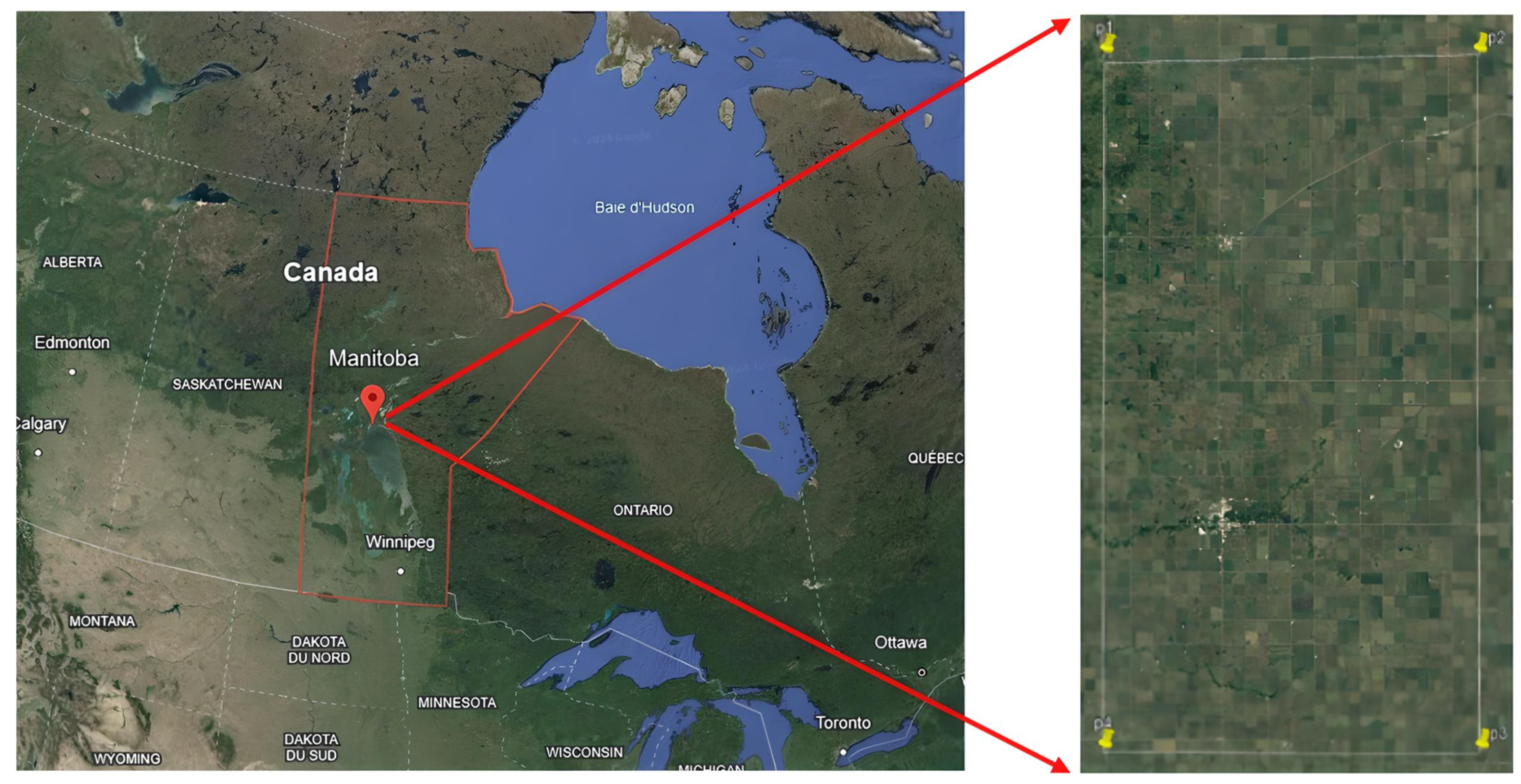
Figure 1. The study area.
Ai 05 00033 g001
Figure 2. Methodology overview.
Ai 05 00033 g002
Figure 3. LST calculation [27].
Ai 05 00033 g003
Figure 4. VWC distribution and thresholds.
Ai 05 00033 g004
Figure 5. CNN-ViT architecture [21].
Ai 05 00033 g005
Figure 6. Feature extractor block.
Ai 05 00033 g006
Figure 7. Visual transformer’s performance.
Ai 05 00033 g007
Figure 8. CNN-ViT’s performance.
Ai 05 00033 g008
Figure 9. Example results of the models. (a) Ground truth label (b) Visual transformer (c) CNN-ViT. (Red colour indicates high-stressed crops, yellow colour shows moderately stressed crops and green colour indicates low-stressed crops.)
Ai 05 00033 g009
Table 1. Landsat 8 bands used in this study. NIR: Near-Infrared; SWIR: Short Wave Infrared.
BandDescriptionWavelength (μm)Resolution (m)
SR-B2Blue (OLI)0.45–0.5130
SR-B3Green (OLI)0.53–0.5930
SR-B4Red (OLI)0.64–0.6730
SR-B5NIR (OLI)0.85–0.8830
SR-B6SWIR1(OLI)1.57–1.6530
SR-B7SWIR2 (OLI)2.11–2.2930
SR-B10Thermal Infrared 1 (TIRS)10.60–11.19100
Table 2. CWSI and VWC thresholds.
CWS ClassCWSI ThresholdCorresponding VWC Threshold (Kg/m2)Number of Elements in the Dataset
Low0 to 0.2> to 2.9613
Moderate0.2 to 0.51.5 to 2.92767
High0.5 to 0.80 to 1.5977
Table 3. Details of the CNN-ViT architecture.
SequenceLayer TypeKernel Size/OperationInput(s)OutputDescription and Details
1Feature Extractor-X_patchFeature MapThe feature extractor takes an image patch as input and extracts spectral and spatial features.
Depth-Wise Convolution block
2DW Convolution 2D(1,1)Feature MapY_1Applies a small, focused filter to the input to detect fine details.
3DW Convolution 2D(3,3)Feature MapY_2Uses a medium-sized filter to capture broader features.
4DW Convolution 2D(5,5)Feature MapY_3Employs a large filter to gather more contextual information.
Combination and Normalisation
5Element-wise Addition-Y_1,Y_2, Y_3YCombines the different detail scales from previous convolutions.
6Normalisation-YNorm(Y)Standardises the feature map to stabilise learning.
7Local Window Attention (LWA)-Norm(Y)LxFocuses on local patterns within the feature map to capture local details and spatial relationships.
Output Processing
8Element-wise Addition-Feature Map, Lx, Norm(Y)ZIntegrates the attention-focused features with the normalised map.
9Normalisation-ZNorm(Z)Further normalises the combined features for the final prediction steps.
Prediction Layers
10Linear Transformation-Norm(Z)Inter. Out 1Transforms features linearly for high-level abstraction.
11Activation function (GELU)-Inter. Out 1Inter. Out 2Applies a non-linear activation function to introduce complexity.
12Linear Transformation-Inter. Out 2OProduces the final output as a prediction probability.
Table 4. Feature extractor block architecture.
SequenceLayer Type/OperationKernel Size/StrideFilter NumbersInput(s)OutputDescription and Details
1Input Reshape--8 × 8 × 88 × 8 × 8 × 1Initial reshape of input data into a 4D tensor.
Input Convolution Layers
23D Convolution1 × 1 × 3168 × 8 × 8 × 18 × 8 × 8 × 16First 3D convolution layer with 16 filters.
33D Convolution1 × 1 × 5328 × 8 × 8 × 168 × 8 × 8 × 32Second 3D convolution layer with 32 filters.
4Reshape to 2D--8 × 8 × 8 × 328 × 8 × 256Reshaping the 3D feature map to 2D for further processing.
Branch F1—Encoder Network
5Separable Conv2D3 × 3328 × 8 × 2568 × 8 × 32First separable 2D convolution in encoder branch.
6Separable Conv2D3 × 3328 × 8×328 × 8 × 32Second separable 2D convolution in encoder branch.
7Max Pooling 2 × 2 (Stride 2)-8 × 8 × 324 × 4 × 32Max pooling reduces spatial dimensions by factor of 2.
Branch F1—Decoder Network
8Transpose Conv2D--4 × 4 × 324 × 4 × 32First transpose convolution in decoder branch.
9Transpose Conv2D--4 × 4 × 324 × 4 × 32Second transpose convolution in decoder branch.
102D Up-sampling--4 × 4 × 328 × 8 × 32Up-sampling to increase spatial dimensions to match input size.
Branch F2
112D Convolution3 × 3/stride 2328 × 8 × 2564 × 4 × 322D convolution with stride reduces dimensions to match output of F1’s encoder.
12Element-wise Addition--4 × 4 × 324 × 4 × 32Summing the outputs of Sequence 7 from F1 and Sequence 11 from F2.
132D Up-sampling (US)--4 × 4 × 328 × 8 × 32Up-sampling to increase spatial dimensions to match input size.
142D Convolution--8 × 8 × 328 × 8 × 32Final 2D convolution layer.
Combination and output
15Element-wise Addition--8 × 8 × 328 × 8 × 32Summing the outputs of the decoder from F1 and F2 and producing the final feature map output.
Table 5. Quantitative results for visual transformer and CNN-ViT on the test data set.
MetricAccuracyPrecisionRecallF1 ScoreCoefficient Kappa
ViT0.88140.87650.82550.85010.7695
CNN-ViT0.90420.87740.88760.88250.8195
Disclaimer/Publisher’s Note: The statements, opinions and data contained in all publications are solely those of the individual author(s) and contributor(s) and not of MDPI and/or the editor(s). MDPI and/or the editor(s) disclaim responsibility for any injury to people or property resulting from any ideas, methods, instructions or products referred to in the content.