A Spatial AI-Based Agricultural Robotic Platform for Wheat Detection and Collision Avoidance

Abstract

To obtain more consistent measurements through the course of a wheat growing season, we conceived and designed an autonomous robotic platform that performs collision avoidance while navigating in crop rows using spatial artificial intelligence (AI). The main constraint the agronomists have is to not run over the wheat while driving. Accordingly, we have trained a spatial deep learning model that helps navigate the robot autonomously in the field while avoiding collisions with the wheat. To train this model, we used publicly available databases of prelabeled images of wheat, along with the images of wheat that we have collected in the field. We used the MobileNet single shot detector (SSD) as our deep learning model to detect wheat in the field. To increase the frame rate for real-time robot response to field environments, we trained MobileNet SSD on the wheat images and used a new stereo camera, the Luxonis Depth AI Camera. Together, the newly trained model and camera could achieve a frame rate of 18–23 frames per second (fps)—fast enough for the robot to process its surroundings once every 2–3 inches of driving. Once we knew the robot accurately detects its surroundings, we addressed the autonomous navigation of the robot. The new stereo camera allows the robot to determine its distance from the trained objects. In this work, we also developed a navigation and collision avoidance algorithm that utilizes this distance information to help the robot see its surroundings and maneuver in the field, thereby precisely avoiding collisions with the wheat crop. Extensive experiments were conducted to evaluate the performance of our proposed method. We also compared the quantitative results obtained by our proposed MobileNet SSD model with those of other state-of-the-art object detection models, such as the YOLO V5 and Faster region-based convolutional neural network (R-CNN) models. The detailed comparative analysis reveals the effectiveness of our method in terms of both model precision and inference speed.

1. Introduction and Motivation

Wheat (Triticum) is one of the most important staple foods in the temperate world, of which the United States produces 8% of the world’s total [1,2,3]. Thus, there is a great need to conduct research on its growth and development in field plot studies conducted as breeding program wheat performance trials. This helps wheat breeders predict plant traits (phenotypes), such as yield, based on their genetic constitutions (genotypes). One of the most important aspects of wheat research is to understand the relationship between wheat growth and the soil properties (for instance, soil moisture) of the fields where it is grown. One measuring device is the Geophex Ltd. Gem-2 electromagnetic induction soil electrical conductivity sensor. It weighs over 15 lbs. and is typically carried manually. To best support digital agricultural research, soil conductivity would be measured several times per week. However, a breeding trial that is $50\mathrm{m}\times 75\mathrm{m}$ can take four hours, and should be done at specific times of day.

To facilitate breeding trials, we used a robot to carry the sensor through a field manually guided via a remote control. The robot saves investigators’ time and energy while trying to acquire the soil’s properties. While remote control provides an easy solution, it is imperative not to inadvertently harm the wheat in any of the three hundred (300) or more plots, which are separated by very constricted aisles (9 to 12 inches). As the field size increases, human control from greater distances becomes hard and the possibility that the robot will run over the wheat increases. One way to avoid this is to make the robots intelligent enough to distinguish the wheat from the aisles, turn its wheels to stay aligned with the aisles (autonomous navigation), and to halt, if, for any reason, that becomes impossible. This requires not only the detection of wheat in the field of view but also its distance from the robot. If the robot recognizes wheat far enough ahead, there is time to align its wheels and avoid collision. However, if the wheat is closer than some permitted threshold distance (for instance, if a surface irregularity unexpectedly deflects the wheels toward the wheat a few feet or inches away at the edge of the aisle), there will not be time to do anything but stop before running over the wheat. This entails the use of spatial artificial intelligence (AI).

Spatial AI is an ability of an AI system to reason based on not just what it is looking at but also how far away things are located. Spatial AI applies AI to not only identify the object but also provide information on where the object, in this case wheat, is in 3D space. When the robot makes the informed decision to halt, the operator and/or the robot itself can turn its wheels, while remaining in place, and then, when they are pointed in the correct direction, restart the acquisition of soil properties.

Our main contributions in this article are as follows:

• Design of an agricultural robotic platform for autonomous navigation in crops while avoiding collisions. The platform uses spatial AI and deep learning models for collision avoidance and crop (wheat) detection.
• Training of different state-of-the-art deep learning models, such as MobileNet single shot detector (SSD), YOLO, and Faster region-based convolutional neural network (R-CNN) with ResNet-50 feature pyramid network (FPN) backbone, for object (wheat) detection.
• Performance comparison of the state-of-the-art deep learning models for wheat detection on different computing platforms.
• Evaluation of the trained deep learning models for wheat detection through various metrics, such as accuracy, precision, and recall.

The remainder of this article is organized as follows. Section 2 summarizes the previous works related to object detection and deep learning, mainly focusing on CNNs. Section 3 discusses the proposed framework and its technical components. Following this, Section 4 discusses training evaluation and detailed experimental results. Finally, Section 5 concludes the article with its limitations and future directions.

2. Related Work

Deep learning has played an important role in various fields, such as biology, medicine, agriculture, and agronomy. This section discusses previous works in the literature related to computer vision and the use of computer vision in agriculture.

Redmon et al. [4] presented YOLO, a new approach in object detection. YOLO treats object detection as a regression problem, which is the main difference between YOLO and prior object detection models. YOLO is very fast, processing images at a higher rate than other object detection approaches, and gives the best performance in real-time object detection [5]. As illustrated in Redmon et al. [4], YOLO reasons globally about the image when making predictions and learns generalizable representations of objects. Results in [4] reveal that YOLO produces only half the number of background errors as compared to Fast R-CNN. These reasons led us to use YOLO as our deep learning model for wheat detection.

Inspired by the work of Ren et al. [6], we also implemented Faster R-CNN with an FPN backbone for real-time wheat detection in the field. Faster R-CNN has achieved state-of-the-art object detection accuracy on PASCAL VOC 2007, PASCAL VOC 2012 [7,8], and MS COCO [9] datasets with only 300 proposals per image. These exceptional results led us to use Faster R-CNN with a ResNet-50-FPN backbone model in our study. Faster R-CNN and RPN have been used by several entries in many competitions [10]. It should also be observed that R-CNN with a ResNet-50-FPN backbone not only provides a cost-efficient solution for practical usage, but also helps improve the accuracy of object detection. Faster R-CNN is composed of two modules. The first module is a deep fully convolutional network and proposes regions, and the second module is the fast R-CNN detector that uses the proposed regions [11]. In this article, the accuracy of YOLO is compared against that of Faster R-CNN with ResNet-50-FPN [12]. This comparison helped us decide which of the two models, that is, Faster R-CNN with ResNet-50-FPN or YOLO, is more suitable for our final implementation in the robotic platform. Results (Section 4.8) reveal that we were able to attain almost equal accuracy using both the models; however, YOLO is faster than Faster R-CNN. A more detailed discussion on the accuracies of the two models is presented in Section 4.10.

Liu et al. [13] have proposed a new approach named single shot detector (SSD), which discretizes the output space of bounding boxes into a set of default boxes with different aspect ratios and scales per feature map location. They observed that the SSD model is relatively simple to train. The SSD model eliminates proposal generation and the subsequent pixel or feature resampling stage and encapsulates all computations in a single network. The work done by He et al. [14] is most relevant to our work. They presented a residual learning framework to ease the training of networks that are substantially deeper than those used in other state-of-the-art models. The extremely deep representations also result in good generalization performance on other recognition tasks, which led them to win 1st place in ImageNet [15] detection, ImageNet localization, and COCO detection competitions. This state-of-the-art performance inspired us to adopt a ResNet backbone in our Faster R-CNN models for wheat detection.

Mosley et al. [16] performed experiments on detecting and counting sorghum head through parameter tuned SSD from the images obtained from unmanned aerial vehicles (UAVs). Their approach involves parameter tuned anchor boxes, which achieves an out-of-sample mean average precision of 0.95. However, their proposed system is unable to work in a real-time environment due to its high computational complexity. Ghosal et al. [17] explored machine learning-based approaches such as deep convolutional neural networks for efficient object detection. Their proposed methodology involves a weakly supervised deep learning framework inspired by active learning for sorghum head detection. They utilized an object detection framework called RetinaNet with ResNet-50. The backbone network adopted in this study was the feature pyramid network (FPN). The FPN was built on top of ResNet-50, and it has shown good results. However, due to complex architecture of ResNet-50, their method cannot be adopted for real-time object detection applications. Velumani et al. [18] have investigated the effect of ground sampling distance (GSD) on detection stage using a Faster R-CNN object detection algorithm for maize plants. Results have shown promising plant detection and counting with a root mean square error of 0.08. However, their method uses a computationally complex ResNet-50 feature extraction backbone in the Retina-Net architecture, which makes their method unsuitable for real-time applications.

Gonzalo-Martín et al. [19] implemented test time augmentation (TTA) to overcome the challenges of differences in shape and color of the sorghum head in UAV imagery. Results indicate that the detection achieved by TTA outperforms detection based on individually transformed testing sets. Xue et al. [20] proposed a velocity control strategy for autonomous agricultural vehicles based on the moment state, hazard severity, and distance between the object and vehicle. Results indicate that their collision avoidance strategy predicts collisions in real-time with an average detection time of 0.2 s. Shutske et al. [21] have developed a microwave sensor and control system to mitigate the probability of a fast-moving vehicle colliding with a slow-moving vehicle from the rear. The sensor unit which is outfitted on the back of a vehicle senses the distance and velocity of a vehicle moving closer from the rear.

Prior works have not leveraged spatial AI and deep learning models for wheat detection and collision avoidance in real-time. Furthermore, previous works did not compare the performances of the state-of-the-art deep learning models for wheat detection on different edge computing platforms. This work filled the void in previous works by devising a real-time wheat detection and collision avoidance system and evaluating the performance of proposed system on a variety of edge computing platforms.

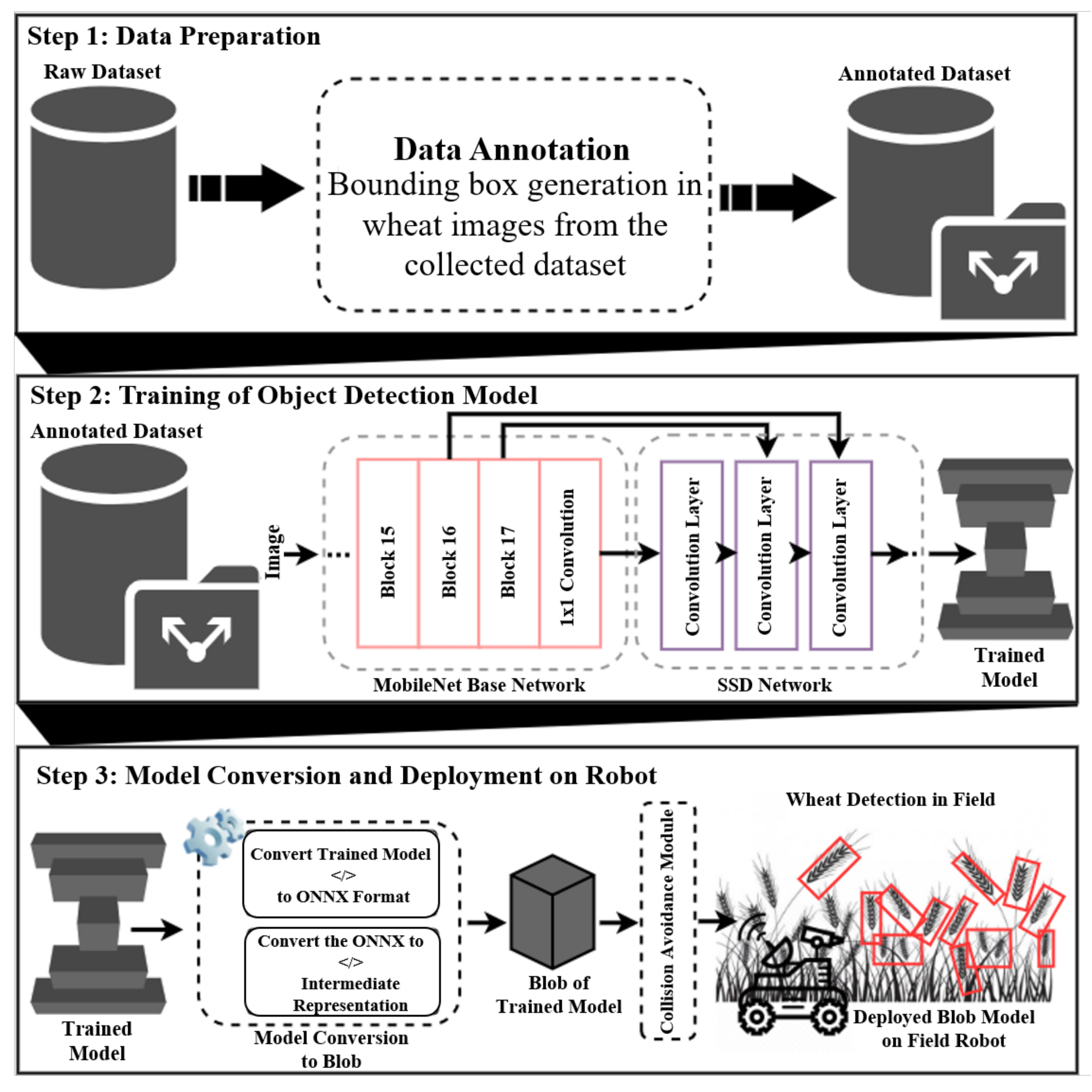
3. Proposed Spatial AI System for Collision Avoidance in Wheat Fields

In this section, we present a detailed discussion of our proposed spatial AI-driven collision avoidance system and its technical components. The workflow of our proposed system was divided into three distinct phases, as shown in Figure 1.

This first phase was the collection of image data for training from different sources, including farm sites and online repositories, such as Google Images and Kaggle. The collected image data were then manually annotated for training by generating bounding boxes on the wheat images. The second phase was the training phase where a computationally efficient yet robust object detector, such as MobileNet SSD, was trained on our prepared annotated dataset. Lastly, the third phase converted the trained wheat detection model to a blob format and then deployed it on the robot for practical use in a real-time application in wheat fields.

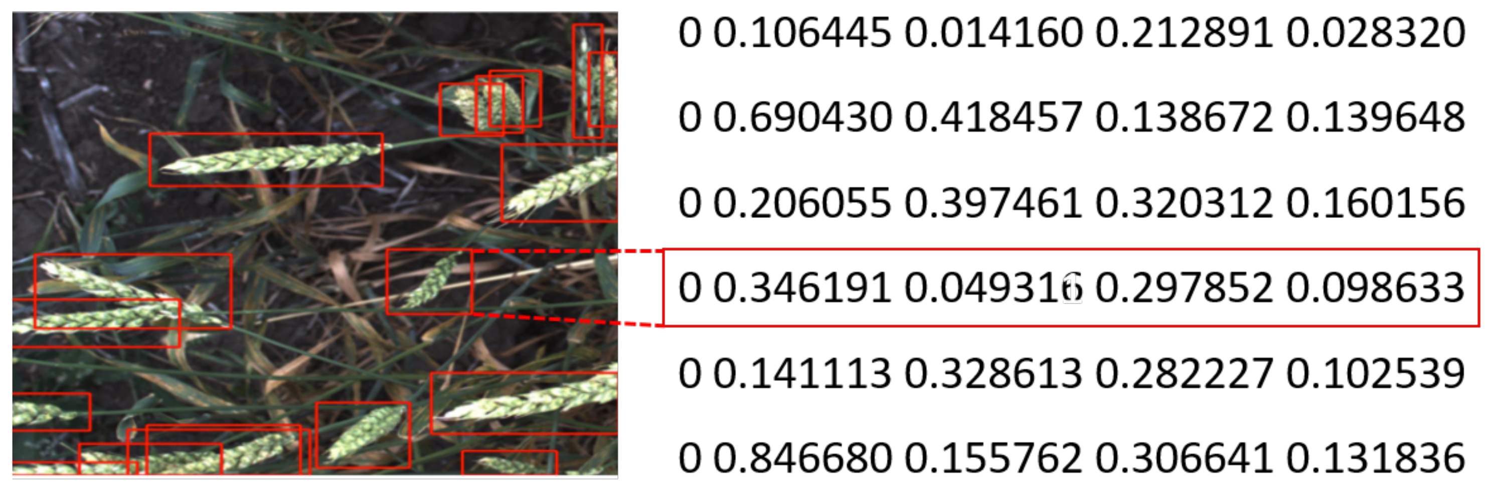
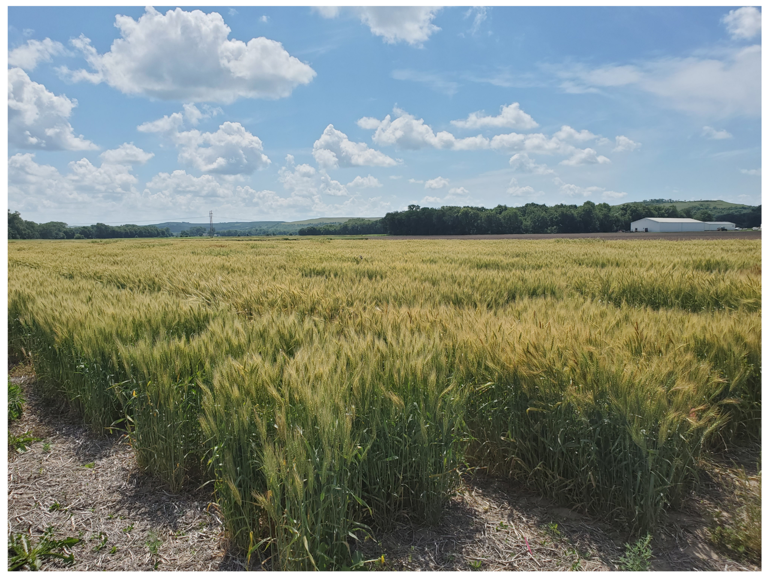
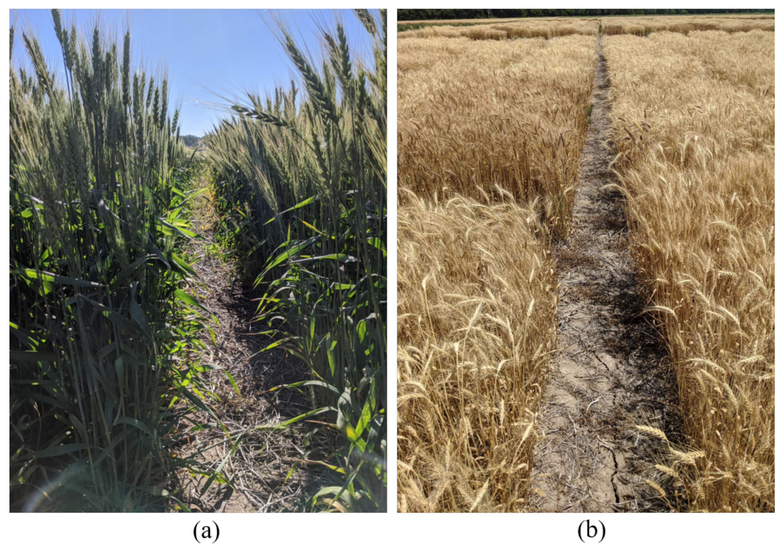
3.1. Data Preparation

In any computer vision problem, the performance of a deep learning model mainly depends on the quality of the dataset, which is, in turn, nothing but the quantity and quality of the images. For training our deep learning model, our dataset comprised images from multiple sources, including farm sites where the robots are used. The data were collected from the field at Ashland bottoms (KSU Agronomy Research Farm) spread over a latitude and a longitude from (39.128, −96.6157) to (39.1284, −96.6164) in the city of Manhattan, Kansas, United States. Most of the images in our collect training dataset were obtained on the KSU Agronomy Farm with a digital camera, as shown in Figure 2. The images were taken considering the view of the robot; that is, the training images are like the images that are to be encountered and predicted by the robot.

One of the important requirements of our deep learning model is that the image recognition must be done in all stages of wheat crop; that is, the wheat color can be brown or green depending on the season or time of operation of the robotic platform. Considering such variety in training data, we collected both brown and green wheat image data from the wheat fields. For ease of understanding, sample images of both brown and green wheat are depicted in Figure 3a,b, respectively. The image shown in Figure 3a was taken on 4 July 2021, and represents the stage of wheat growth called the reproductive stage. This is the stage where the wheat heads have fully emerged from the stem. Pollination is very quick and takes only 3 to 5 days to complete. Thus, the images were taken in quick succession, forming a dataset comprising 1200 images of pollinated wheat with emerged heads. The image shown in Figure 3b was taken on 22 June 2021. This stage of wheat growth is called the maturity stage, which is also known as hard dough. In this phase, the plant turns a straw color and the kernel becomes very hard. The focus of collected training images is to get view of robot and make sure that wheat is clearly visible and can be annotated for training. In addition, we also collected images from online public repositories, such as Google Images and Kaggle. From Google Images, we downloaded non-copyrighted images, including both brown and green wheat images. From the Kaggle repository, we acquired more than 3000 images, and this amount was later increased by performing data augmentation before training the model. After collecting the dataset, we manually annotated the collected images by labeling them with bounding boxes (rectangles) having four coordinates that specify the locations of wheat in the given image. A bounding box specifies the region of interest by (x, y) coordinates of the upper-left corner and the (x, y) coordinates of the lower-right corner, which together define a diagonal representation of a rectangle. The sample annotation of bounding boxes over a wheat image is depicted in Figure 4.

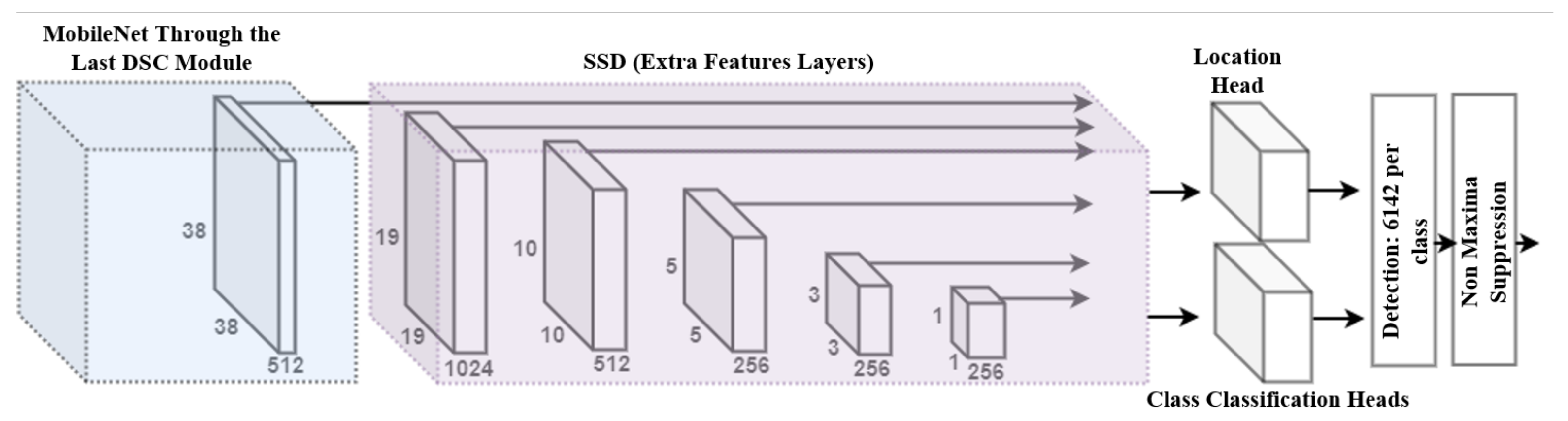
3.2. MobileNet SSD Architecture for Wheat Detection

In this research study, we explored different state-of-the-art object detection models, including YOLO v5, Faster R-CNN, and MobileNet SSD, and compared their performances for wheat detection. Based on the obtained performance, we determined that the MobileNet SSD is better than other models in terms of objection detection accuracy, model complexity, and time complexity. Therefore, we chose MobileNet SSD as the object detection architecture in our proposed framework (Figure 1) for wheat detection in the field. A detailed discussion on the proposed MobileNet SSD architecture is provided in the subsequent subsection.

3.2.1. Architectural Details of MobileNet SSD

This section provides the technical details of the MobileNet SSD architecture employed in our proposed spatial AI system for wheat detection and collision avoidance. The MobileNet SSD architecture is an encapsulation of two modules that include a backbone feature extraction module and an SSD module (containing extra object-specific feature extraction layers), as depicted in Figure 5. The MobileNet V1 backbone feature extractor uses depthwise separable convolutions instead of standard convolutions, where each depthwise separable convolution layer consists of depthwise and pointwise convolutions, which greatly reduces the overall complexity of model. The standard MobileNet V1 architecture starts with a standard convolution layer, followed by 13 depth convolution layers. After the depthwise separable convolution layers, the obtained features maps are converted to a fully connected layer and pooled by a maxpooling layer, and finally the softmax layer generates the probabilities for a predefined number of classes based on the extracted features. Since here our objective is to use only the learned representation from the MobileNet V1 architecture, we froze the last three layers (fully connected layer, maxpooling layer, and softmax layer) and used the output from the last depthwise convolutional layer, and fed that to the SSD detector module as an input.

The SSD detector module first applies a set of boxes to each cell of the feature maps learned from the MobileNet V1 architecture. Next, it predicts a score for each candidate class in the corresponding feature map cell. Consequently, for each map, SSD generates $(C_{candidate}+4)/kwh$ results, where $C_{candidate}$ denotes number of classes, k represents the number of default bounding boxes, and w and h represent the width and height of feature map, respectively. The SSD architecture uses several feature maps having different resolutions to take advantage of both low-level and high-level features. Based on the utilized feature maps in the SSD architecture, the scale of the default box $S_k$ can be mathematically expressed as follows:

$$S_k=S_{min}\frac{S_{max}-S_{min}}{m-1}\times (k-1)$$

(1)

where $S_{min}$ and $S_{max}$ are the scales of the lowest and highest feature map, respectively, and m represents the number of features maps. The five common aspect ratios of bounding boxes can be expressed as $A_R\in \{1,2,3,0.5,0.33\}$, where the width and height of the box can be computed using $S_k\sqrt{A_R}$. Similarly, the center of a bounding box can be estimated as $\left(\frac{i+0.5}{|f_k|},\frac{j+0.5}{|f_k|}\right)$, where $|f_k|$ is the size of feature maps and $i,j\in [0,|f_k\left|\right]$. Further, SSD uses a Jaccard index metric to compute the matches, where the Jaccard value ≥ 0.5 between the ground-truth and the predicted bounding boxes is considered to be a match box. Mathematically, the Jaccard index metric can be expressed as follows:

$$Jaccard=\frac{A_o}{A_u}$$

(2)

where $A_o$ denotes the area of overlap (i.e., the common area between the ground-truth and the predicted bounding box) and $A_u$ denotes the area of union (i.e., combined area of the ground-truth and the predicted bounding box), respectively.

The SSD architecture uses the joint loss function which is the summation of localization loss $L_{loc}$ and classification loss $L_{cls}$. The localiztaion loss is smooth L1 loss ($L{1}_{smooth}$), which can be mathematically expressed as follows:

$$\begin{array}{cc}\hfill & L_{loc}(x,l,g)=\sum _{i\in Pos}^N\sum _{m\in \{cx,cy,w,h\}}{x}_{ij}^{k}L{1}_{smooth}(l_i^m-{\widehat{g}}_j^m),\hfill \\ \hfill & \mathrm{where}\hfill \\ \hfill & {\widehat{g}}_j^{cx}=\frac{g_j^{cx}-d_i^{cx}}{d_i^w},{\widehat{g}}_j^{cy}=\frac{g_j^{cy}-d_i^{cy}}{d_i^h},{\widehat{g}}_j^w=log\left(\frac{g_j^w}{d_i^w}\right),{\widehat{g}}_j^h=log\left(\frac{g_j^h}{d_i^h}\right).\hfill \end{array}$$

(3)

Here, N is the number of correct matches, and the terms d, g, and l represent the default bounding box, ground-truth bounding box, and predicted bounding box, respectively. The symbols $cx$ and $cy$ represent the x and y coordinates, respectively, of the center location of the default bounding box, and w and h denote the width and height of the default bounding box, respectively.

The second type of loss that SSD uses is classification loss $L_{cls}$, which is the loss function related to the prediction of the object type by the predicted bounding box. The classification loss of SSD can be mathematically expressed as follows:

$$L_{cls}(x,c)=-\sum _{i\in Pos}^N{x}_{ij}^{p}log\left({\widehat{c}}_i^p\right)-\sum _{i\in Neg}log\left({\widehat{c}}_i^0\right)$$

(4)

where the term ${\widehat{c}}_i^p=\frac{exp\left(c_i^p\right)}{{\sum }_{p}exp\left(c_i^p\right)}$ represents the model’s predicted confidence score for class p. The term ${\widehat{c}}_{i^0}$ represents the confidence value for the negative match of the bounding box. Similarly, $Pos$ and $Neg$ represent the positive and negative matches of bounding boxes, respectively. The term $x_{ij}^p$ is an indicator variable which verifies the match of the ith default bounding box and the jth ground-truth bounding box for class p. Together with both loss functions, the joint loss function $Los{s}_{total}$ can be calculated as follows:

$$Los{s}_{total}=\frac{1}{N}\left(L_{cls}(x,c)+\alpha L_{loc}(x,l,g)\right)$$

(5)

where N denotes the total number of correct matches and $\alpha$ represents the weight factor for the localization loss.

3.2.2. Motivation of Using MobileNet SSD for Wheat Detection

The selection of a suitable model for the problem under consideration is very challenging, particularly when the computing resources onboard the robot are limited. This section briefly discusses the reasons why we have chosen a MobileNet SSD architecture over YOLO V5 and Faster R-CNN architectures for our spatial AI-based framework. Several factors, such as model complexity, model accuracy, and model inference time, need to be considered while dealing with resource-constrained computing platforms and their usage for practical industrial applications, such as agriculture. To choose a suitable optimal object detection model, we have conducted extensive experiments and evaluated MobileNet SSD, YOLO V5, and Faster R-CNN models based on the aforementioned criteria. Based on the detailed model evaluation experiments (Section 4), we chose MobileNet SSD for our proposed framework, as MobileNet SSD model balances tradeoffs between model accuracy, model complexity, and inference time. Furthermore, MobileNet SSD is feasible for computing platforms with limited memory and resources, such as LattePanda, Raspberry Pi, and Intel Neural Compute Stick.

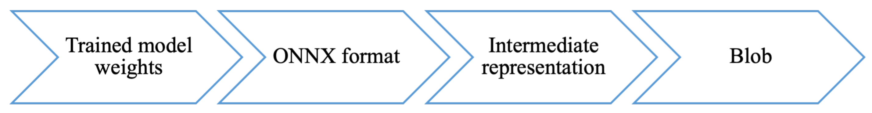
3.3. Model Conversion and Deployment on Field Robot

In this section, we discuss the conversion of the trained model to a blob format and its deployment on a robot for real-time wheat detection in the field. The proposed model conversion module is three-fold, which converts network binaries at three levels and obtains the final blob representation of the trained model, as shown in Figure 6. The model conversion module starts with the input trained model and converts it into an open neural network exchange (ONNX) format. The model conversion module encode the model’s metadata in protocol buffer format (having extension .proto), which provides only the data type information (e.g., float32) of the trained model layers and learned knowledge in a JSON file. The next level of conversion is an intermediate representation, which is an ad hoc extraction of the ONNX information designed to facilitate its conversion to the final blob format. To enable the use of custom-trained models by DepthAI [22], converting them into a blob file format optimizes the best inference on Myriad X processor. The first three steps in model conversion pipeline are coded using open source modules publicly available in Python; the last step (also programmed in Python) is done via an online API call to software provided by Luxonis [23].

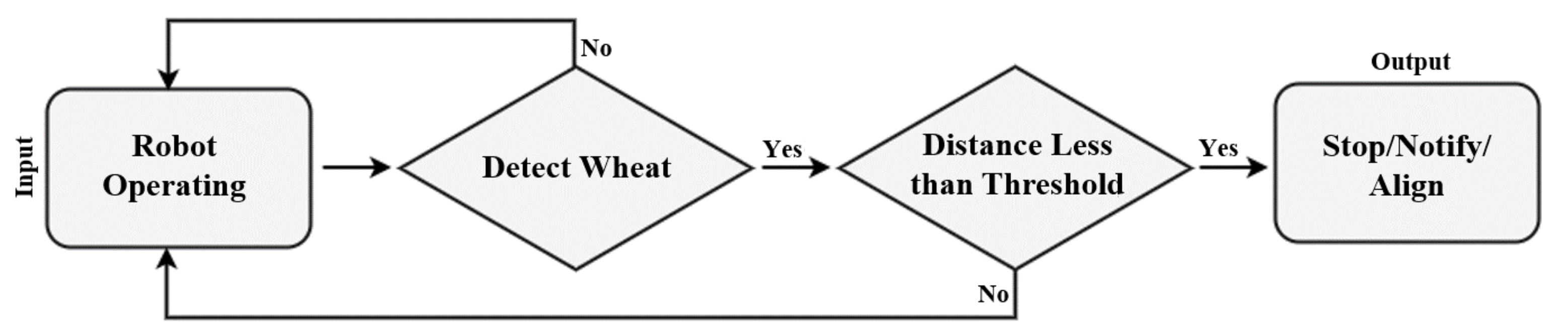
3.4. Workflow for Robot Operation and Collision Avoidance

In this section, we discuss the decision-making and collision avoidance workflow of a robot for wheat detection in field. The robot used in this research was equipped with a stereo camera [24] and the trained model. For better understanding, the operations of our proposed robotic system are put into two categories, namely, wheat detection and collision avoidance. The first category of robot operation is wheat detection, where the mounted stereo camera, along with the trained model, helps the robot to not only detect the wheat in the field but also supervises it to drive on the right path in the field to avoid collisions. The second category of robot operation is to avoid collisions with wheat via depth sensing and communication between the robot and the embedded computing device using the PySerial API. Both collision avoidance through depth sensing and communicating via PySerial API are discussed in detail the following subsections.

3.4.1. Collision Avoidance via Depth Sensing

The above section described how the object detection is achieved. However, the final decision on when to stop the robot is solely based on the distance between wheat and the robot. Thus, the depth information is crucial. To acquire depth sensing, left and right stereo cameras outfitted on the OpenCV AI kit [24] were utilized, and the object detection was accomplished by the red, green, blue (RGB) camera outfitted at the center of the OpenCV AI kit. An OpenCV AI kit was put on the robot. The OpenCV AI camera neither uses weights of the model nor the model directly to perform object detection; rather, it uses a blob which was obtained from the OpenVINO model. The blob conversion is accomplished using open source software provided by Luxonis [23], as discussed in Section 3.3. The obtained blob is then used in detecting wheat, and left and right stereo cameras of the OpenCV AI kit are used in estimating the distance of wheat from the camera (and thus the robot).

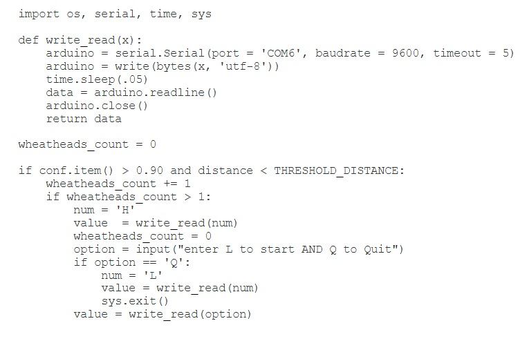
3.4.2. Communicating with the Robot Using PySerial

To stop the robot when it detects wheat at less than the threshold distance, a connection needs to be established between the robot and the embedded controller board (LattePanda [25] in the case of our implementation). LattePanda has a Universal Serial Bus (USB) port, which is connected to the Arduino controller of the robot. When the deep learning model detects wheat, it sends a signal to the USB port, via which the signal is sent to the robot’s speed controller, which adjusts the robot’s speed. A flowchart of this process is shown in Figure 7, and the related code snipped for robot control is shown in Figure 8. This code snippet is embedded into depth-sensing code for communicating with the robot. In the code, “conf” represents the confidence of object detection, whose threshold can be adjusted by the designer depending on the performance of the model.

4. Training Evaluation and Experimental Results

This section provides a detailed discussion on the training phase of this research study. First, we discuss data augmentation as a preprocessing step. Next, we present the embedded computing platforms with which we performed feasibility analysis to determine their suitability for deployment on our robotic system. We then briefly discuss the evaluation metrics for performance evaluation and comparison, followed by training details of MobileNet SSD and other comparative object detection models (YOLO V5 and Faster R-CNN).

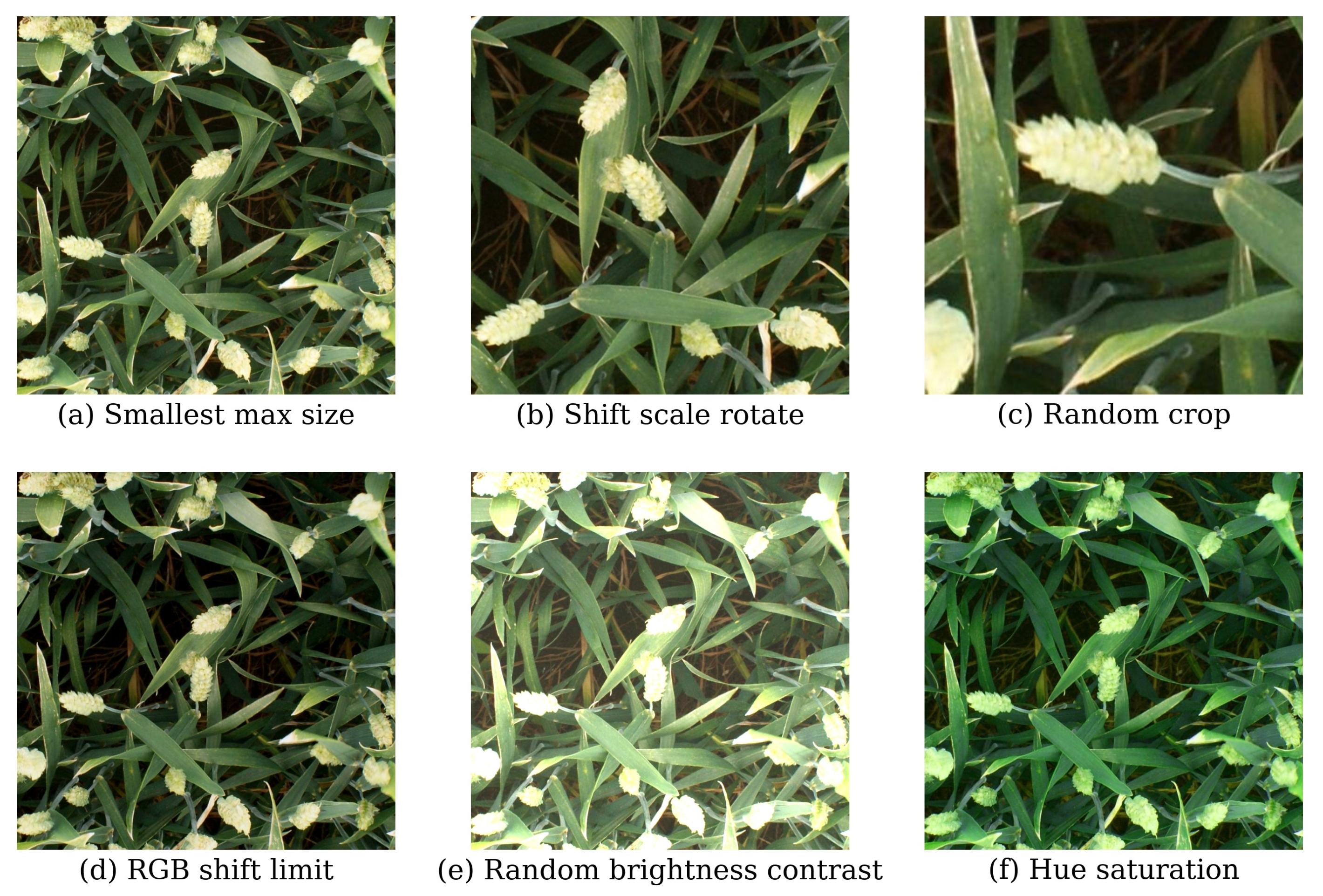
4.1. Data Augmentation

Image augmentation is the process of taking the images that are already present in the training dataset and manipulating them to create various altered versions of the same image. Augmentation provides more images to train and gives a different viewpoint to the classifier. Different viewpoints can represent changes in the saturation, color, crop, and horizontal and vertical flips. To create augmented data, we used a PyTorch orientation module named Albumentations. Albumentations is a module where all the necessary augmentation steps for augmentations are provided in predefined functions. These functions are applied to the image dataset to create manipulated images, which are then used for training the deep learning model. A few examples of augmentations applied are:

SmallestMaxSize: Rescales an image so that the minimum size is equal to the given maximum size, while keeping the aspect ratio of the initial image.

ShiftScaleRotate: Randomly assigns transforms, such as translate, scale, and rotate, to the input images.

RandomCrop: Crops a random part of the image.

RGBshift: Randomly shifts values for each channel of the input RGB image.

RandomBrightnessContrast: Randomly changes brightness and contrast of the input image.

The transformations of training image after data augmentations are visually depicted in Figure 9.

4.2. Embedded Computing Platforms

We benchmarked the deep learning models on various embedded computing platforms that are suitable for integration with the robotic platform for wheat detection. The embedded computing platforms that we leveraged in our experimentation and benchmarking included LattePanda, Intel Neural Compute Stick (NCS), and OpenCV AI kit. Here, we summarize the main characteristics of these embedded computing platforms.

4.2.1. LattePanda

LattePanda Alpha 864s [25] is a high-performance, palm-sized embedded board that runs Windows 10 and has low power consumption. It is being widely utilized in edge computing, vending, advertising machines, and industrial automation. This palm-sized machine was outfitted onto our autonomous robot and was used for running the deep learning model(s), communicating with the operator, and communicating with the robot’s integral components. Key features of LattePanda Alpha 864s are an Intel Core M3-8100Y dual-core processor operating at 1.1–3.4 GHz, an Intel Ultra High Definition (UHD) Graphics 615, 8 GB Memory, and an integrated Arduino ATMEL 32U4 co-processor.

4.2.2. Intel Neural Compute Stick

Intel NCS [26] is an accelerator for deep learning to enable the deep learning model to recognize objects at a high rate of frames per second. It can support heterogeneous execution across computer vision accelerators implemented on a central processing unit (CPU), graphics processing unit (GPU), vision processing unit (VPU), and field-programmable gate array (FPGA). It supports the Intel OpenVINO toolkit, and also supports various operating systems, including Windows, Mac, and Ubuntu. It integrates an Intel Movidius Myriad X VPU. It supports various machine learning frameworks, including TensorFlow, Caffe, Apache MXNet, Open Neural Network Exchange (ONNX), PyTorch, and PaddlePaddle via an ONNX conversion.

4.2.3. OpenCV AI Kit

OpenCV AI Kit with Depth (OAK-D) [24] is a spatial AI platform that can simultaneously run advanced neural networks while providing depth from two 1 megapixel (MP) global shutter-synchronized stereo cameras, one on the left and one on the right, and color information from a single 4K 12 MP RGB camera in the center. OAK-D is essentially a smart camera with neural inference and depth processing capability. OAK-D can be used with any host operating system that OpenVINO supports. It supports 4K/30 fps H.265, JPEG, H.264, and H.265/HEVC encodings [27].

4.3. Evaluation Metrics

In the following, we discuss the evaluation metrics we have utilized for evaluating our deep learning models.

4.3.1. Precision

Precision P measures the accuracy of a model’s prediction; that is, precision quantifies the percentage of correct predictions [28].

$$P=\frac{TP}{TP+FP}$$

(6)

where $TP$ denotes true positives, that is, predicted as positive correctly; and $FP$ denotes false positives, that is, predicted as positive, incorrectly.

4.3.2. Recall

Recall R measures how well a model finds all the positives [28]:

$$R=\frac{TP}{TP+FN}$$

(7)

where $TP$ signifies true positives, that is, predicted as positive correctly, and $FN$ represents false negatives, that is, predicted as positive, incorrectly.

4.3.3. Intersection over Union (IoU)

An object detection system’s predictions are characterized by a bounding box and a class label [28]. For each bounding box, the measure of correctness is defined by an IoU metric, which measures the overlap between the predicted bounding box and the ground truth bounding box; that is,

$$IoU=\frac{A_o}{A_u}$$

(8)

where $A_o$ and $A_u$ are area of overlap and the area of union, respectively. For object detection tasks, precision P and recall R are calculated using the $IoU$ for a given $IoU$ threshold. For example, if $IoU$ prediction is greater than the $IoU$ threshold, then we classify that prediction as true positive ($TF$). If the $IoU$ value for a prediction is less than 0.5, say 0.4, we classify that prediction as a false positive ($FP$). This implies that for a given prediction, we may get different binary $TP$, $FP$, and false negative ($FN$) values, and thus different P and R values, by changing the $IoU$ threshold.

4.3.4. Mean Average Precision (mAP)

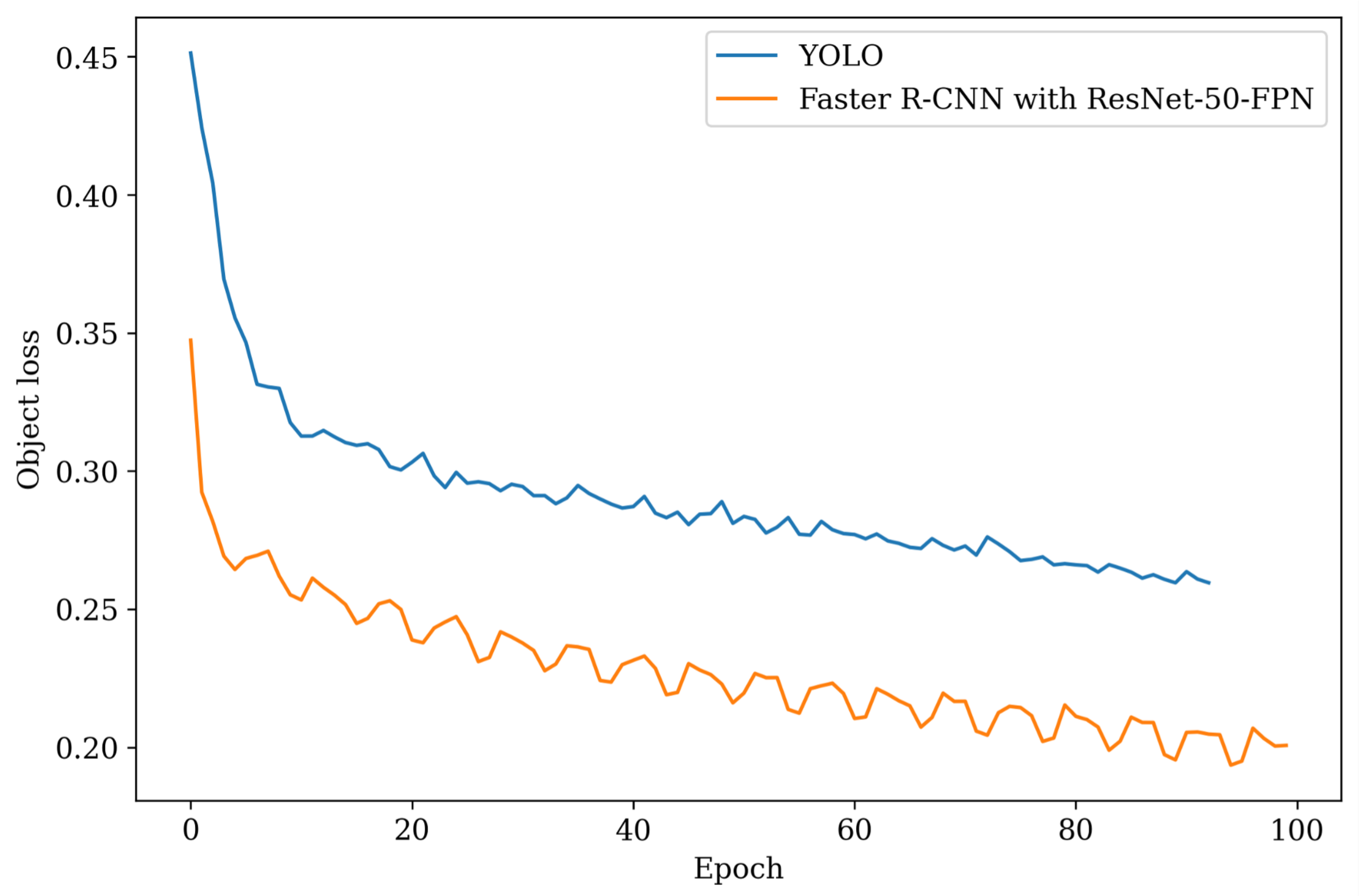
The average precision (AP) for a given class is obtained by calculating the area under the precision–recall (PR) curve for the object detections. The mAP is the average of AP over all classes and/or overall $IoU$ thresholds for a set of detections. Often, interpolated AP, in particular, 11-point interpolated AP, is used for calculating mAP.

4.4. Training YOLO

The final and the most crucial part of creating a real-time deep learning model is to train the model on training images. YOLO performs supervised training for object detection. We performed the training of our YOLO model in Google Collaboratory using Colab Pro subscription. Google Collaboratory provides Nvidia Tesla K80 GPUs that have a dual-GPU design with 4992 CUDA cores (2496 CUDA cores per GPU). Nvidia Tesla K80 has a 24 GB of GDDR5 memory and has a PCI Express (PCIe) interface. For every cycle of data collected from the KSU Agronomy Farm, YOLO was trained on approximately 2000+ images for 7.679 h of GPU time. The training was performed on a pretrained model with available weights of a large YOLO model. As the new images were added to the dataset, training was performed on the new images to update the model weights. The training, validation, and testing splits for different data sources are given in

Table 1. Training, validation, and testing splits (%) for different data sources.

Image Source	Training	Validation	Testing
Kaggle	80	10	10
Google Images	80	10	10
KSU Agronomy Farm	70	10	20

. Training was done by setting image size to $1024\times 1024$, batch size to 16, and the number of training epochs to 100.

4.5. Training Faster R-CNN with ResNet-50-FPN

We have used stochastic gradient descent (SGD) as an optimizer in training this model. The learning rate (LR) scheduler used in training this model was step LR. The loss function used in the Faster R-CNN was binary cross-entropy in the first state of the region proposal network (RPN), and the classification loss used was normal cross-entropy [6]. Training was performed in Google Collaboratory. The initial training of Faster R-CNN with ResNet-50-FPN took 8 h of GPU time for 2000+ images. Object loss comparison between YOLO and Faster R-CNN with ResNet-50-FPN while training is shown in Figure 10. To insure the timely convergence and avoid over-fitting, we used an “early stop” strategy that allows one to stop the training if the model converges well-enough and there is no room for further improvement in training and validation losses.

4.6. Training MobileNet SSD

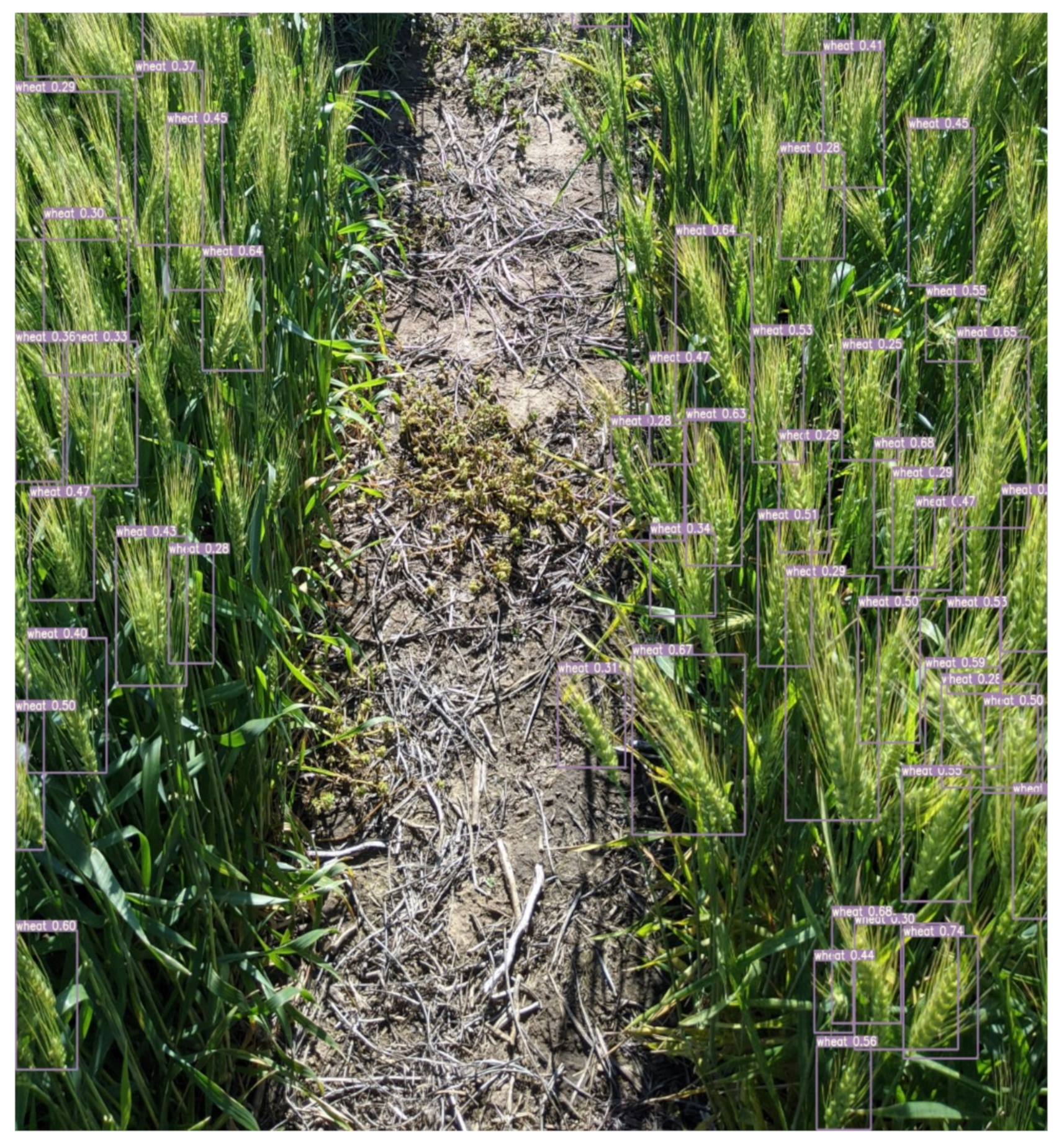
The anticipation and classification of bounding box positions in SSD architecture was done in a single pass by a single convolutional network in the SSD architecture. The network consists of a base architecture followed by several convolution layers. Originally, MobileNet SSD model was trained on a benhmark object detection dataset called “COCO dataset”. In this research, we used the pre-trained MobileNet SSD model and retained it on our wheat images dataset using a transfer learning approach. We utilized Tensorflow object detection API and Model Zoo resources for training MobileNet SSD and other two object detection models, including YOLO V5 and Faster R-CNN. The MobileNet SSD, due to its single shot approach to recognizing several objects in the image, is faster as compared to two-shot RPN based approaches, such as R-CNN. TensorFlow Object Detection API is a framework designed to solve object detection problems. Model Zoo consists of pretrained computer vision models on the COCO dataset and the KITTI dataset.

4.7. Testing YOLO

To test the performance of YOLO, the model was run on test images from the dataset. The performance of the model $P_m$ is defined by the following equation.

$$P_m=\frac{N_D}{N_T}$$

(9)

where $N_D$ denotes the total number of wheat heads detected and $N_T$ denotes the total number of wheat heads present in the image. Our YOLO model achieved a performance of 0.93 on the test dataset. The weights of this model were saved for future training and inference in the field.

4.8. Testing Faster R-CNN with ResNet-50-FPN

Our Faster R-CNN with ResNet-50-FPN model achieved a performance of 0.90 (using Equation (9)) in identifying the wheat heads. Results indicate that the performance of YOLO is 3.33% higher as compared to the Faster R-CNN with ResNet-50-FPN. Testing was done on LattePanda [29], which is the actual embedded computing platform used for real-time detection in the field.

4.9. Testing MobileNet SSD

We have evaluated the accuracy of our MobileNet SSD model using our images collected from the Agronomy farm (Figure 2). Results indicate that MobileNet SSD attained accuracy close to those of Faster R-CNN with ResNet50 FPN and YOLO. Results show that MobileNet SSD caused a slight decrease in detection accuracy: 5% and 3% as compared to YOLO and Faster R-CNN, respectively. Since the major concern in this study was to attain high speed inference on embedded platforms, we deployed MobileNet SSD on the OpenCV AI kit. Results reveal that the model achieved 12–13 fps on $600\times 600$ images and 18–23 fps on $300\times 300$ image.

4.10. Comparing YOLO, Faster-R-CNN, and MobileNet SSD

After training both YOLO and Faster R-CNN with ResNet-50-FPN on the training dataset, results revealed that the models attained almost identical performance results in terms of wheat head detection (Equation (9)). Results further indicate that the speed of YOLO is three times faster than that of the Faster R-CNN with ResNet-50-FPN. Figure 11 shows time taken in seconds by the three deep learning models to perform inferences for various numbers of images.

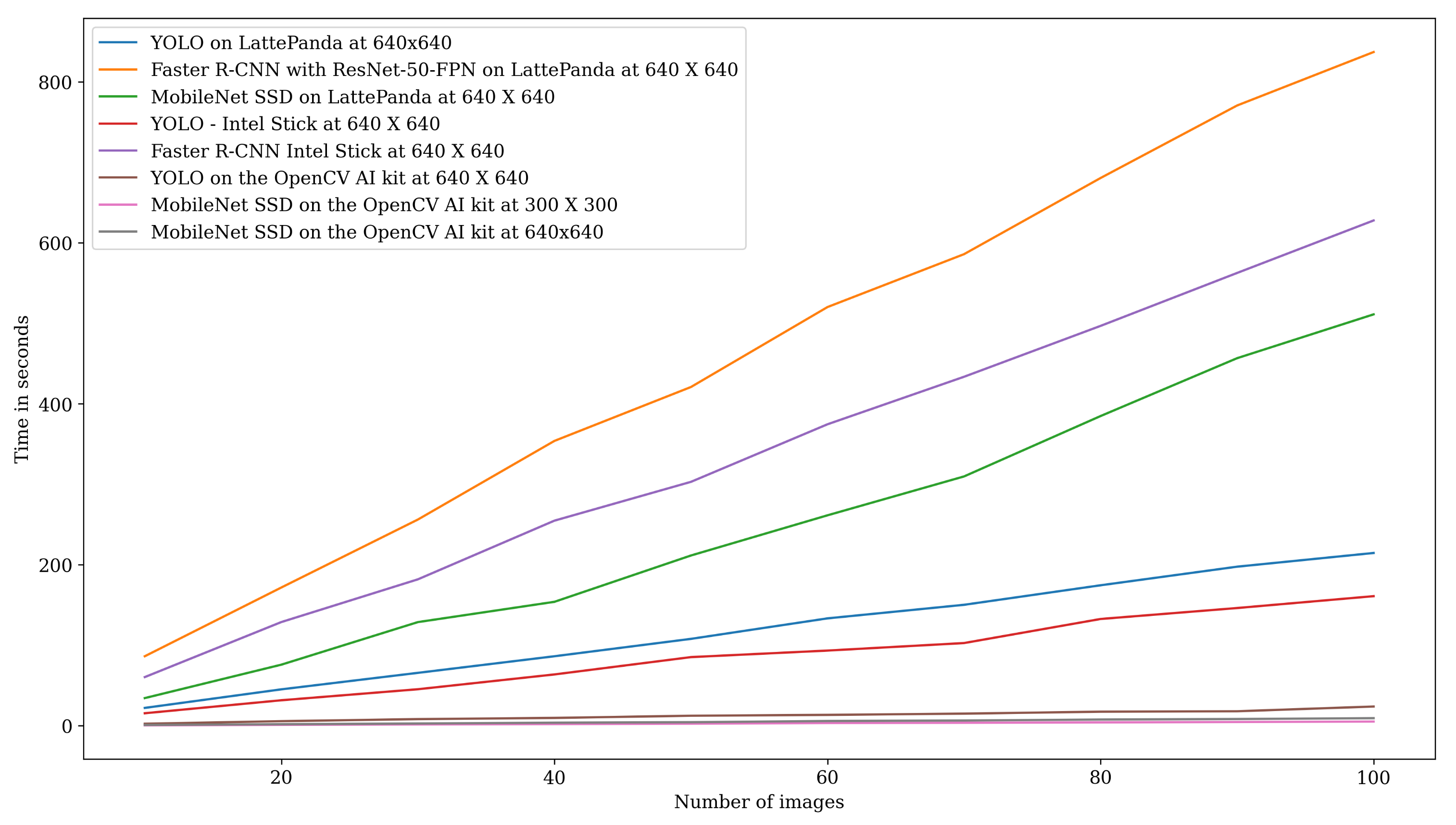
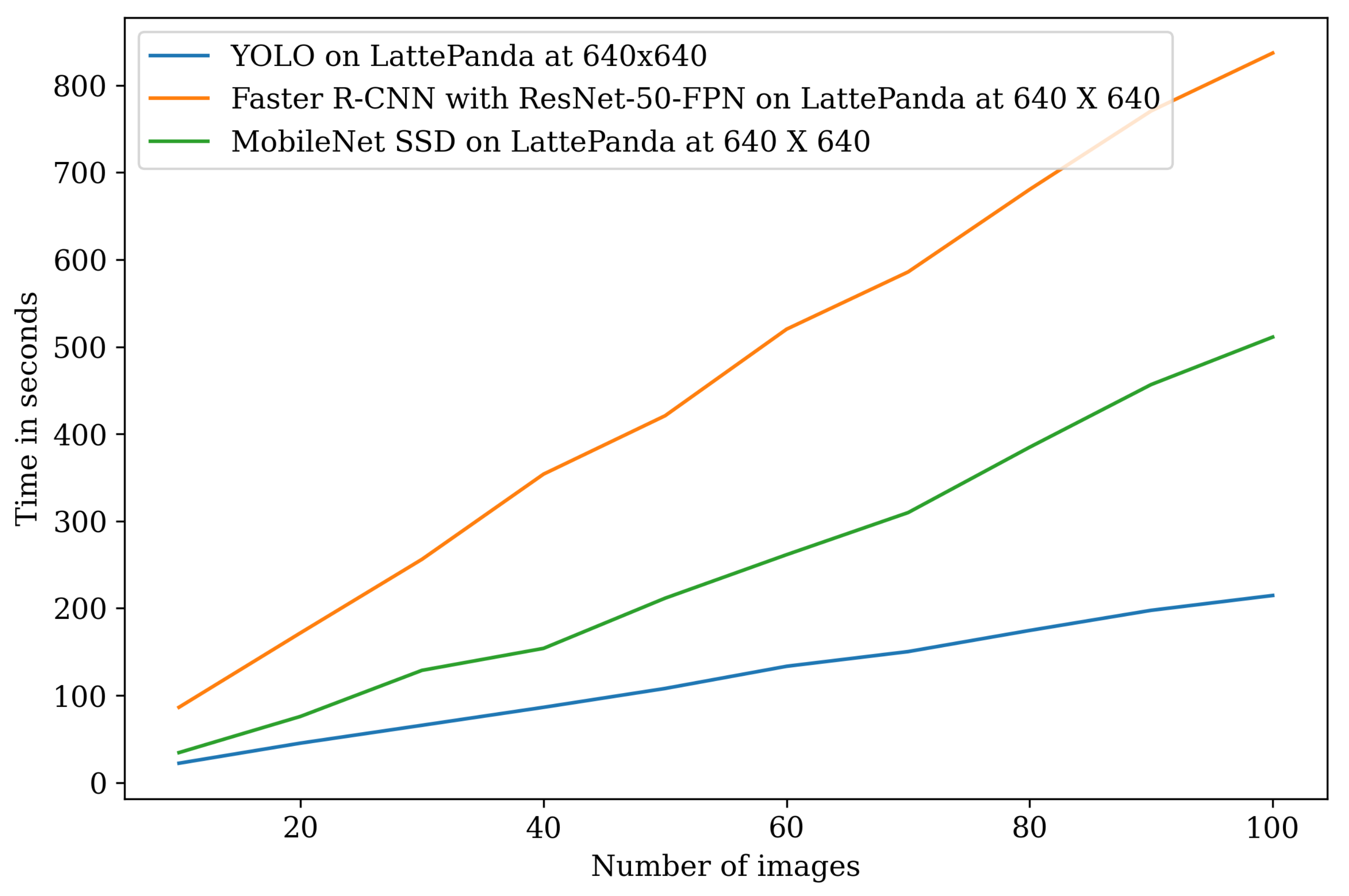
4.11. Benchmarking Deep Learning Models on Various Embedded Computing Platforms

Figure 12 and

Table 2. Time taken to perform wheat detection on various platforms.

Images	YOLO on LattePanda at 640 × 640	Faster R-CNN on LattePanda at 640 × 640	MobileNet SSD on LattePanda 640 × 640	YOLO on Intel Stick 640 × 640	Faster R-CNN on Intel Stick 640 × 640	YOLO on OpenCV AI Kit at 640 × 640	MobileNet SSD on OpenCV AI Kit at 640 × 640	MobileNet SSD on OpeCV AI Kit at 300 × 300
10	22.13	86.33	34.33	15.49	60.43	2.4	0.93	0.52
20	45.19	171.74	75.85	31.63	128.80	5.64	1.88	0.52
30	65.68	256.17	128.74	45.32	181.88	8.21	2.77	1.55
40	86.31	353.87	153.94	63.71	254.79	9.69	3.76	2.06
50	107.91	420.85	211.5	84.24	303.01	12.40	4.38	2.56
60	133.38	520.19	261.43	93.36	374.53	13.47	5.85	3.31
70	150.23	585.90	309.73	102.70	433.56	15.02	6.48	3.64
80	174.49	680.53	384.76	132.62	496.79	17.44	7.65	4.14
90	197.60	770.64	456.66	146.22	562.57	17.96	8.35	4.63
100	214.36	837.08	511.13	160.97	627.81	23.84	9.37	5.15

depict the time taken in seconds to perform inferences for various number of images on different embedded computing platforms. The deep learning models that we benchmarked included YOLO, Faster R-CNN with ResNet-50-FPN, and MobileNet SSD. The embedded computing platforms on which these models were run included Intel stick, OpenCV AI kit, and LattePanda. Results indicate that MobileNet SSD on the OpenCV AI kit at an image size of $300\times 300$ achieved the lowest inference time, whereas Faster R-CNN with ResNet-50-FPN at an image size of $640\times 640$ resulted in the highest inference time among the compared models.

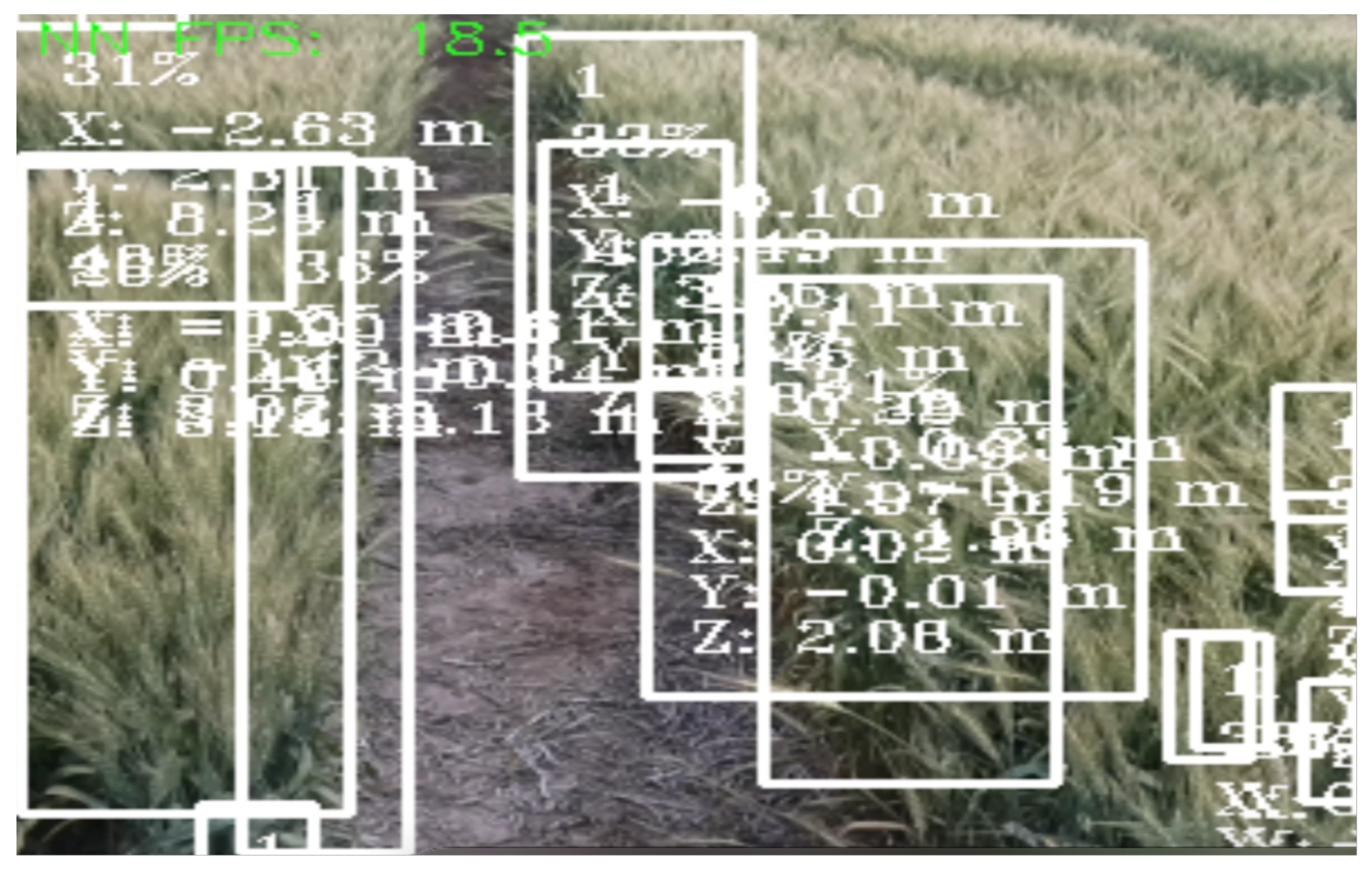
4.12. In-Field Real-Time Object Detection and Depth Sensing

The performances of our object detection and depth-sensing models were tested in the KSU Agronomy Farm (Figure 2) where the robot was deployed. As indicated above, MobileNet SSD was used for real-time object detection in the field. The results of object detection are shown in Figure 13, and the results of depth sensing are shown in Figure 14. The effectiveness of the wheat recognition can be increased by varying the threshold/confidence level of the model.

5. Conclusions

In this study, we designed an autonomous robotic platform that performs collision avoidance while navigating in crop rows using spatial AI. We explored and compared various deep learning models to determine the models that can provide high accuracy and inference speed on relatively low-cost embedded devices, such as LattePanda, Intel Neural Compute Stick, and OpenCV AI Kit, which are suitable for integrating on the robotic platform. We trained a MobileNet SSD architecture and other comparative object detection models, YOLO V5 and Faster R-CNN, on our prepared wheat images dataset. The experimental results revealed that the MobileNet SSD model attained the best detection performance on LattePanda for wheat detection with the runner-up inference speed (YOLO V5 was fastest), thereby dominating Faster R-CNN model in terms of both model detection accuracy and inference speed. Thus, MobileNet SSD achieves a better trade-off between model accuracy and time-complexity. Furthermore, results indicate that MobileNet SSD outperforms YOLO V5 on OpenCV AI Kit in terms of both model accuracy and inference speed. These results indicate that the MobileNet SSD model is a suitable candidate for real-time applications on resource-constrained computing platforms by providing stable accuracy and fast inference speeds. After these experimental evaluations, the trained MobileNet SSD model was combined with the stereo depth sensing on OpenCV kit mounted on our robotic platform to detect the distances of the objects (i.e., wheat) from the camera to avoid collision with wheat.

The current work had limitations, such as (i) not making the robot fully autonomous, and (ii) not identifying alleys present in the field. These limitations can be eliminated by using segmentation techniques to detect alleys in the field and making the robot fully autonomous using path planning algorithms, such as the dynamic window collision approach. Path planning algorithms can be combined with deep learning models to achieve fully autonomous driving of the robot. In the future, we plan to include a segmentation-based approach for path identification, which will make our robot more intelligent while moving in the field for wheat detection.

References

1. Asseng, S.; Ewert, F.; Martre, P.; Rötter, R.P.; Lobell, D.B.; Cammarano, D.; Kimball, B.A.; Ottman, M.J.; Wall, G.; White, J.W.; et al. Rising temperatures reduce global wheat production. Nat. Clim. Chang. 2015, 5, 143–147. [Google Scholar] [CrossRef]
2. Tack, J.; Barkley, A.; Nalley, L.L. Effect of warming temperatures on US wheat yields. Proc. Natl. Acad. Sci. USA 2015, 112, 6931–6936. [Google Scholar] [CrossRef] [PubMed]
3. Ihsan, M.Z.; El-Nakhlawy, F.S.; Ismail, S.M.; Fahad, S.; Daur, I. Wheat phenological development and growth studies as affected by drought and late season high temperature stress under arid environment. Front. Plant Sci. 2016, 7, 795. [Google Scholar] [CrossRef] [PubMed]
4. Redmon, J.; Divvala, S.; Girshick, R.; Farhadi, A. You only look once: Unified, real-time object detection. In Proceedings of the IEEE Conference on Computer Vision and Pattern Recognition, Las Vegas, NV, USA, 27–30 June 2016; pp. 779–788. [Google Scholar]
5. Srivastava, S.; Divekar, A.V.; Anilkumar, C.; Naik, I.; Kulkarni, V.; Pattabiraman, V. Comparative analysis of deep learning image detection algorithms. J. Big Data 2021, 8, 1–27. [Google Scholar] [CrossRef]
6. Ren, S.; He, K.; Girshick, R.; Sun, J. Faster R-CNN: Towards real-time object detection with region proposal networks. Adv. Neural Inf. Process. Syst. 2015, 28, 91–99. [Google Scholar] [CrossRef] [PubMed]
7. Everingham, M.; Van Gool, L.; Williams, C.K.; Winn, J.; Zisserman, A. The pascal visual object classes (voc) challenge. Int. J. Comput. Vis. 2010, 88, 303–338. [Google Scholar] [CrossRef]
8. Everingham, M.; Eslami, S.A.; Van Gool, L.; Williams, C.K.; Winn, J.; Zisserman, A. The pascal visual object classes challenge: A retrospective. Int. J. Comput. Vis. 2015, 111, 98–136. [Google Scholar] [CrossRef]
9. Lin, T.Y.; Maire, M.; Belongie, S.; Hays, J.; Perona, P.; Ramanan, D.; Dollár, P.; Zitnick, C.L. Microsoft coco: Common objects in context. In European Conference on Computer Vision; Springer: Cham, Switerland, 2014; pp. 740–755. [Google Scholar]
10. ImageNet Large Scale Visual Recognition Challenge 2015 (ILSVRC2015). Available online: https://www.image-net.org/challenges/LSVRC/ (accessed on 16 August 2022).
11. Girshick, R. Fast r-cnn. In Proceedings of the IEEE International Conference on Computer Vision, Santiago, Chile, 7–13 December 2015; pp. 1440–1448. [Google Scholar]
12. Tan, M.; Le, Q. Efficientnet: Rethinking model scaling for convolutional neural networks. In Proceedings of the 36th International Conference on Machine Learning, Long Beach, CA, USA, 9–15 June 2019; ML Research Press: Maastricht, The Netherlands, 2019; pp. 6105–6114. [Google Scholar]
13. Liu, W.; Anguelov, D.; Erhan, D.; Szegedy, C.; Reed, S.; Fu, C.Y.; Berg, A.C. SSD: Single shot multibox detector. In Proceedings of the European Conference on Computer Vision, Munich, Germany, 8–14 September 2016; Springer: Cham, Switerland, 2016; pp. 21–37. [Google Scholar]
14. He, K.; Zhang, X.; Ren, S.; Sun, J. Deep residual learning for image recognition. In Proceedings of the IEEE Conference on Computer Vision and Pattern Recognition, Las Vegas, NV, USA, 27–30 June 2016; pp. 770–778. [Google Scholar]
15. Krizhevsky, A.; Sutskever, I.; Hinton, G.E. Imagenet classification with deep convolutional neural networks. Adv. Neural Inf. Process. Syst. 2012, 25, 1097–1105. [Google Scholar] [CrossRef]
16. Mosley, L.; Pham, H.; Bansal, Y.; Hare, E. Image-based sorghum head counting when you only look once. arXiv 2020, arXiv:2009.11929. [Google Scholar]
17. Ghosal, S.; Zheng, B.; Chapman, S.C.; Potgieter, A.B.; Jordan, D.R.; Wang, X.; Singh, A.K.; Singh, A.; Hirafuji, M.; Ninomiya, S.; et al. A weakly supervised deep learning framework for sorghum head detection and counting. Plant Phenomics 2019, 2019, 1525874. [Google Scholar] [CrossRef] [PubMed]
18. Velumani, K.; Lopez-Lozano, R.; Madec, S.; Guo, W.; Gillet, J.; Comar, A.; Baret, F. Estimates of maize plant density from UAV RGB images using Faster-RCNN detection model: Impact of the spatial resolution. arXiv 2021, arXiv:2105.11857. [Google Scholar] [CrossRef] [PubMed]
19. Gonzalo-Martín, C.; García-Pedrero, A.; Lillo-Saavedra, M. Improving deep learning sorghum head detection through test time augmentation. Comput. Electron. Agric. 2021, 186, 106179. [Google Scholar] [CrossRef]
20. Xue, J.; Xia, C.; Zou, J. A velocity control strategy for collision avoidance of autonomous agricultural vehicles. Auton. Robot. 2020, 44, 1047–1063. [Google Scholar] [CrossRef]
21. Shutske, J.M.; Gilbert, W.; Morgan, S.; Chaplin, J. Collision avoidance sensing for slow moving agricultural vehicles. Pap.-Am. Soc. Agric. Eng. 1997, 3. Available online: https://www.researchgate.net/publication/317729198_Collision_avoidance_sensing_for_slow_moving_agricultural_vehicles (accessed on 16 August 2022).
22. Luxonis. DepthAI’s Documentation. 2022. Available online: https://docs.luxonis.com/en/latest/ (accessed on 4 August 2022).
23. Luxonis. Luxonis-Simplifying Spatial AI. 2021. Available online: https://www.luxonis.com/ (accessed on 4 August 2022).
24. OpenCV. OpenCV AI Kit: OAK-D. 2021. Available online: https://store.opencv.ai/products/oak-d (accessed on 4 August 2022).
25. LattePanda. LattePanda Alpha 864s. 2021. Available online: https://www.lattepanda.com/products/lattepanda-alpha-864s.html (accessed on 4 August 2022).
26. Intel. Intel Neural Compute Stick. 2021. Available online: https://www.intel.com/content/www/us/en/developer/tools/neural-compute-stick/overview.html (accessed on 4 August 2022).
27. Naushad, R. Introduction to OpenCV AI Kits (OAK-1 and OAK-D). 2021. Available online: https://medium.com/swlh/introduction-to-opencv-ai-kits-oak-1-and-oak-d-6cdf8624517 (accessed on 4 August 2022).
28. Yohanandan, S. mAP (mean Average Precision) Might Confuse You! 2020. Available online: https://towardsdatascience.com/map-mean-average-precision-might-confuse-you-5956f1bfa9e2 (accessed on 7 December 2021).
29. LattePanda Alpha 864s (Win10 Pro activated)—Tiny Ultimate Windows/Linux Device. Available online: https://www.dfrobot.com/product-1729.html (accessed on 16 August 2022).
Figure 1. The visual overview of our proposed spatial AI system for collision avoidance in wheat field.
Ai 03 00042 g001
Figure 2. Research site (KSU Agronomy farm) in Manhattan, Kansas.
Ai 03 00042 g002
Figure 3. The visual overview of wheat at different states. (a) A sample image from the KSU Agronomy Farm when wheat is in reproductive state. (b) A sample image from the KSU Agronomy Farm when wheat is in mature state.
Ai 03 00042 g003
Figure 4. The visual depiction of sample annotated image from training data.
Ai 03 00042 g004
Figure 5. The visual overview of the MobileNet SSD architecture employed in our proposed framework.
Ai 03 00042 g005
Figure 6. The visual overview of workflow for model conversion to blob format.
Ai 03 00042 g006
Figure 7. Workflow for robot’s operation and collision avoidance.
Ai 03 00042 g007
Figure 8. Code snippet to perform collision avoidance.
Ai 03 00042 g008
Figure 9. Sample images from the augmented training dataset.
Ai 03 00042 g009
Figure 10. Object loss for YOLO and Faster R-CNN with ResNet-50-FPN.
Ai 03 00042 g010
Figure 11. Time taken to perform wheat detection.
Ai 03 00042 g011
Figure 12. Time taken to perform wheat detection on various platforms.
Ai 03 00042 g012
Figure 13. Real-time detection of wheat heads in the field.
Ai 03 00042 g013
Figure 14. Real-time depth sensing of wheat in the field.
Ai 03 00042 g014