Augmented Air Traffic Control System—Artificial Intelligence as Digital Assistance System to Predict Air Traffic Conflicts

Abstract

Today’s air traffic management (ATM) system evolves around the air traffic controllers and pilots. This human-centered design made air traffic remarkably safe in the past. However, with the increase in flights and the variety of aircraft using European airspace, it is reaching its limits. It poses significant problems such as congestion, deterioration of flight safety, greater costs, more delays, and higher emissions. Transforming the ATM into the “next generation” requires complex human-integrated systems that provide better abstraction of airspace and create situational awareness, as described in the literature for this problem. This paper makes the following contributions: (a) It outlines the complexity of the problem. (b) It introduces a digital assistance system to detect conflicts in air traffic by systematically analyzing aircraft surveillance data to provide air traffic controllers with better situational awareness. For this purpose, long short-term memory (LSTMs) networks, which are a popular version of recurrent neural networks (RNNs) are used to determine whether their temporal dynamic behavior is capable of reliably monitoring air traffic and classifying error patterns. (c) Large-scale, realistic air traffic models with several thousand flights containing air traffic conflicts are used to create a parameterized airspace abstraction to train several variations of LSTM networks. The applied networks are based on a 20–10–1 architecture while using leaky ReLU and sigmoid activation function. For the learning process, the binary cross-entropy loss function and the adaptive moment estimation (ADAM) optimizer are applied with different learning rates and batch sizes over ten epochs. (d) Numerical results and achievements by using LSTM networks to predict various weather events, cyberattacks, emergency situations and human factors are presented.

1. Introduction

When Orville and Wilbur Wright first took off with the Wright Flyer in 1903, they were the only ones in the sky. More than a century later, in 2019, a new daily peak of 37,200 flights were counted in the European total network manager area [1]. The global COVID-19 pandemic has brought air traffic to almost a complete standstill in recent years [2,3]. Nevertheless, the number of flights is steadily rising again. Forecasts predict a recovery in the medium term [3]. Alongside this development, an upward trend can be observed by the variety of aircraft such as specialized operations (SPOs) and unmanned aircraft systems (UASs) accessing the European airspace. With the above increases, today’s human-centric air traffic management (ATM) system is reaching its limits. ATM can be divided into three main services, air traffic services (ATS), air traffic flow management (ATFM), and airspace management (ASM) [4]. Air traffic control (ATC) is part of ATS. ATM evolves around air traffic controllers and pilots and has made air traffic remarkably safe in the past.

However, the amount of data that air traffic controllers have to deal with increases proportionally with air traffic. Consequently, information overload and the resulting stress can severely affect mental and physical health, which in turn reduces cognitive performance and impairs decision-making ability. A further difficulty is airspace utilization. European airspace is fragmented in zones and divided along national borders. Each zone contains sectors managed by air traffic controllers. Surveillance technologies such as primary surveillance radio detection and ranging (RADAR) (PSR) [5] and secondary surveillance RADAR (SSR) [6] are used to monitor aircraft on the ground and in the sky. Direct voice communications via very-high-frequency (VHF) and HF radio are used to make tactical interventions and provide the flight crew with the necessary information (flight information service (FIS)) throughout the entire flight.

Aviation is a complex system in which many people work closely together and depend on each other to ensure safe and efficient operations. This human-centered design poses significant problems such as congestion, deterioration of flight safety, greater costs, more delays, and higher emissions. Transforming the ATM into the “next generation” requires complex human-integrated systems that provide better abstraction of airspace and create situational awareness, as described in the literature for this problem [7,8,9,10].

This research outlines the complexity of the problem and introduces a digital assistance system called an augmented ATC (AATC) system to detect conflicts in air traffic by systematically analyzing aircraft surveillance data to provide air traffic controllers with better situational awareness. In particular, the system monitors aircraft on the ground and in the air and informs the air traffic controller of emerging issues related to potential conflicts in air traffic. For this purpose, long short-term memory (LSTM) networks, which are a popular version of recurrent neural networks (RNN), a kind of deep sequential neural network, are used to determine whether their temporal dynamic behavior is capable to reliably monitor air traffic and classify error patterns [11,12,13,14]. LSTM networks are able to cope with the vanishing gradient problem, classify, process, and make predictions on sequential data or time series, since there may be delays of unknown duration between important events in a time series. Large-scale, realistic air traffic models with several thousand flights containing air traffic conflicts are used to create a parameterized airspace abstraction to train several variations of LSTM networks. To generate a large amount of structured data to ensure that the LSTM networks are exposed to many different circumstances to identify patterns and trends by adjusting its biases and weights, the air traffic simulation and modeling framework developed in previous research was used [15]. In this context, a user-defined number of flights with a selection of pseudo-randomly weighted air traffic conflicts are generated. The datasets exposed to the LSTM networks contain realistic air traffic models with a corresponding percentage of manipulated flights [16,17]. Regarding weather events, the dataset contains 34.26% manipulated flights. For cyberattacks on aircraft and ground infrastructure, the dataset for jamming includes 27.99%, for deleting, 27.98%, for spoofing, 28.10%, and for injecting, 32.85% manipulated flights. The dataset for emergency situations contains 36.66%, for deliberate actions, 34.98%, and for technical malfunctions, 36.24% of manipulated flights. Finally, the datasets for human factors include 36.20% wrong set squawk, 35.53% horizontal position (POS) deviation, and 35.36% altitude (ALT) and speed (SPD) deviations. The applied LSTM networks are based on a 20–10–1 architecture while using leaky ReLU and sigmoid activation function. For the learning process, the binary cross-entropy loss function and the adaptive moment estimation (ADAM) optimizer are applied with different learning rates and batch sizes over ten epochs. The numeric results show that the temporal dynamic behavior of the applied LSTM networks have high potential to reliably monitor air traffic and classify error patterns to provide better situational awareness to air traffic controllers. More precisely, the final training accuracy for all simulated cyberattacks against aircraft and ground infrastructure, emergency situations, deliberate actions, technical malfunctions, and various human factors is around 99% with low losses (<0.2). In terms of weather events, a final training accuracy of about 90% is achieved with a model loss of less than 0.3. At this point, it should be noted that everything within this research project was programmed with Python, Tensorflow, Keras, and scikit-learn.

The paper is structured as follows: An outline of the complexity of the problem in the introduction and background section is followed by a factual description of air traffic conflicts, the generation of large-scale, realistic air traffic models, and data preprocessing. The next two sections focus on the background and theory of RNN and on the analysis of the applied variants of LSTM networks trained with the appropriate datasets. At the end, a conclusion is drawn.

2. Related Work

The Single European Sky (SES) initiative was launched by the European Commission (EC) in the year 2000 to modernize, reorganize, and improve European airspace. As part of SES, the SES ATM Research (SESAR), formerly known as SESAME, which represents the ATC infrastructure modernization program, was established. Out of SESAR, the so-called European ATM master plan emerged. It can be considered as a road map for the “next generation” European ATM system. Moreover, it shows the willingness of all stakeholder groups to modernize, reorganize, and improve European airspace. Nevertheless, progress is very slow. The original SES vision was to improve safety performance by a factor of 10, reduce the environmental impact of flights by 10%, reduce the cost of ATM services to airspace users by at least 50%, and triple capacity when needed, all by the year 2020. It is worth noting that none of the aforementioned objectives have been fully realized. European airspace is still fragmented in zones and divided along national borders. Each zone is further subdivided into sectors managed by an air traffic controller. All these factors contribute to congestion, deterioration of flight safety, greater costs, more delays, and higher emissions [7,8].

Aviation has become one of the safest means of transport, due in part to ATM’s human-centered design. However, with the increase in air traffic and the variety of airspace users, the amount of data that air traffic controllers have to deal with increases proportionally. Consequently, information overload and the resulting stress can severely affect mental and physical health, which in turn reduces cognitive performance and impairs decision-making ability. This demonstrates the importance of moving ATM into the “next generation”. Previous research shows that complex human-integrated systems are needed to provide better abstraction of airspace and create situational awareness [9,10].

In recent decades, remarkable academic research has been conducted in the field of artificial intelligence (AI). Deep learning (DL), which is a subset of machine learning (ML) methods based on artificial neural networks (ANNs), achieves great power and flexibility by learning from big data. DL architectures such as deep neural networks (DNNs), convolutional neural networks (CNNs), or RNNs have been used in many scientific fields to improve automation and perform analytical and physical tasks. These include brain tumor detection [18], weather forecasts [19], earthquake signal classification [20], modeling magnetic signature of spacecraft equipment using multiple magnetic dipoles [21], traffic flow prediction [22], electricity price forecasting [23], or generally for weak signal detection [24], to name a few. In aviation, research such as the big data platform of ATM [25], air traffic controllers workload forecasting method based on NNs [26], resilient communication network of ATM systems [27], aviation delay estimation using DL [28], collaborative security management [29], research status of ANNs and its application assumption in aviation [30], human–human collaboration to guide human–computer interaction design in ATC [31], design of integrated air/ground automation [32], or safety and human error in automated air traffic control [33] reflects great potential of automation to solve complex problems.

To fill the scientific gap and find out whether DL techniques and corresponding optimization techniques are also suitable as digital assistance systems for air traffic controllers to monitor airspace and predict emerging air traffic conflicts, this research was initiated. As aircraft surveillance data are time series data, RNN models, especially LSTM networks, are investigated and applied on generated air traffic data.

3. Background

Intelligence can be seen as the ability to learn and apply appropriate techniques to solve problems and achieve goals in an ever-changing and uncertain world. Evolution has perfectly developed humans over millions of years to recognize the visual world and adapt to new circumstances. When you read this sentence, you will understand the content based on the word order without having to think about each word from scratch. DL, a type of ML and AI, is a biologically inspired programming paradigm to improve automation and perform analytical and physical tasks without human intervention [34].

DL is essentially a network with an input, hidden, and output layer that continuously adapts to new circumstances by learning from data. It is important to note that there can only be one input layer and one output layer. However, the number of hidden layers can vary and is theoretically unlimited. The series of layers is called depth, and each layer can contain a certain number of neuron-like cells called width. 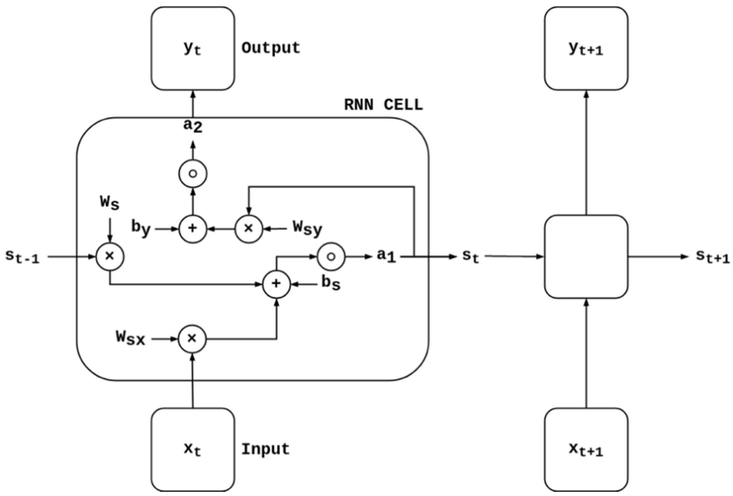Ordinary feedforward ANNs are designed for data points that are independent of each other [35]. When it comes to sequential or time series data, where one data point depends on the previous data point, the network has to be modified to incorporate the dependencies between these data points. RNN is a class of ANN adapted to work with sequential or time series data. It can be trained to hold states or information about preceding inputs to produce the next output of the sequence (see Figure 1). In the feedforward pass of an RNN, the activation vector $s_t$ stores the values of the hidden cells and the output y at time t. The activation vector $s_0$ is initialized to zero, and an iteration regarding the time t over the subsequent hidden layers takes place. Finally, the last layer computes the output y of the RNN for the t-th time step. The output layer is similar to an ordinary layer of a traditional feedforward ANN. The current data point or input x of each individual cell at time t is a scalar value with a d-dimensional feature vector. Each cell consists of three weights. Weights are real values associated with each feature. They are coefficients that are associated with the RNN and are shared temporally to indicate the relevance of the feature to predict the final value. The weight $W_{sx}$ is associated with the input of the cell in the recurrent layer. The weight $W_s$ is associated with the hidden cells, and the weight $W_{sy}$ is associated with the output of the cells. Regarding the bias vector, $b_s$, which is associated with the recurrent layer, and $b_y$, which is associated with the feedforward layer, are temporally shared coefficients. These coefficients are used to shift the activation functions $a_1$ and $a_2$ to the left or right. The activation functions are used for nonlinear transformation of the input and output and decide whether a cell should be activated or not. They enable the network to learn and perform more complex tasks. Different layers can have different activation functions. As part of this research, the leaky rectified linear unit (ReLU) and the sigmoid activation functions are chosen (see Section 5).

The state $s_t$ of a cell can be calculated as follows [12]:

$$s_t=a_1\left(W_s{s}_{t-1}+W_{sx}{x}_t+b_s\right)$$

(1)

The two cross-products of the weight $W_s$ and cell state $s_{t-1}$, and the weight $W_{sx}$ and the current data point or input vector $x_t$, are added to the bias $b_s$. The result is then multiplied by the activation function $a_1$. Consequently, the output of the cell $y_t$ is expressed as follows [12]:

$$y_t=a_2\left(W_{sy}{s}_t+b_y\right)$$

(2)

The cross-product corresponds to the product of the weight $W_{sy}$ and the state $s_t$ of the cell. It will be summed up with the bias $b_y$ and finally multiplied with the second activation function $a_2$. The simplest type of an RNN is a one-to-one architecture expressed as $T_x=T_y=1$. Within this research, a many-to-one architecture (see Figure 2) is chosen based on the defined aircraft attributes outlined in Section 4. This type of RNN, described as $T_x>1, T_y=1$, is usually used for sentiment classification.

To optimize the network, the so-called loss function L (see Equation (3) [12]) is introduced. It serves as a scalar-valued metric to determine how far the predicted output of the network deviates from the true output. That means it indicates how well or poorly a model behaves at each time step when confronted with a particular dataset. The sum of errors made for each example is calculated as follows:

$$L\left(\widehat{y},y\right)={{\displaystyle \sum }}_{t=1}^{T_y}L\left({\widehat{y}}_t,y_t\right)$$

(3)

For the classification task within the developed AATCS, the binary cross-entropy is chosen (see Section 5). This task answers the question with only two choices (i.e., 0 or 1). Besides the loss function, the cost function is applied to the entire training set or a batch (gradient descent). It is a method to measure the performance of a network. In particular, it measures the error between the prediction value of the network and the actual value represented as a single real number. The purpose of this error function is to find the values of the model parameters, for which it provides either the smallest possible number or the largest possible number. The update of weights and biases are based on the error at the output. This process is called backpropagation. It is performed at each point in time T. The derivative of the loss function L with regards to the weight matrix W (all weights of each layer) is calculated as follows [12]:

$$\frac{\partial L_T}{\partial W}={{\displaystyle \sum }}_{t=1}^T\frac{\partial L_T}{\partial W}|\left(t\right)$$

(4)

This fine-tuning allows lower error rates and improves the reliability of the model by increasing generalization. Activation functions allow backpropagation as gradients, which are supplied along with the error at the output to update weights and biases accordingly.

4. Generation and Processing of Air Traffic Datasets with Air Traffic Conflicts

Reliable data are an essential element that enables AI to detect and classify air traffic conflicts. In the course of this research, weather events, cyberattacks against aircraft and ground infrastructure, emergency situations, and human factors are considered as air traffic conflicts.

To obtain sufficient structured data to create a parameterized airspace abstraction, a numerical computer-based air traffic simulation and modeling framework developed in previous research was used [15]. Withal, each flight consists of a fixed number of 100 data samples, where each data sample contains 11 quality attributes, also referred to as features. These attributes include aircraft surveillance information such as the sample number (SN), planned flight path (FP), call sign (CS), 24-bit Mode S address, squawk, barometric altitude (ALT), indicated air speed (IAS), magnetic heading (MH), latitude (LAT) and longitude (LON) information for the horizontal position (POS), and the ATC compliance.

To generate a user-defined number of flights with a selection of pseudo-randomly weighted air traffic conflicts, individual flight models with different flight profiles are used [15,16,17]. Each simulated flight receives an individual CS and 24-bit Mode S address. In terms of weather-related events, such as turbulence, thunderstorms, hail, volcanic ash, or even low visibility, the aircraft is guided around by modifying the waypoints and interpolating the FP. Cyberattacks such as jamming, deleting, spoofing, or injecting may paralyze airspace and compromise flight safety by intercepting and modifying automatic dependent surveillance broadcast (ADS-B) traffic. During a jamming attack, all affected CS, 24-bit Mode S address, squawk, ALT, IAS, MH, LAT, and LON variables in a random weighted interval are erased. The erased values are then displayed as “−1”. Deleting attacks need a certain number of variables in a specific data sample over a randomly weighted interval to erase the dedicated variables. On the other hand, spoofing modifies the variables of the features ALT, IAS, LAT, and LON over a random weighted interval. An injecting attack presented as ghost flight modifies CS, 24-bit Mode S address, squawk, ALT, IAS, MH, LAT, and LON variables over a random weighted interval. FP and ALT are interpolated in a straight-line-on-a-sphere-way between two defined positions using coordinate manipulation. Injecting malicious ADS-B messages can fool ATC and other airspace users into thinking a ghost flight is a normal flight. Emergency situations are often associated with technical malfunctions of an aircraft and deliberate actions in the sense of malicious intent. For this reason, missing data during take-off, climb, cruise, descent, and approach are taken into account. In case of an emergency, three defined transponder (XPDR) codes are reserved to inform the air traffic controller without voice communication. The first reserved XPDR code is 7500, which is used in case of hijacking or other unlawful interference. The second one is 7600, used for a loss of communications, while the last one is 7700, used for a general emergency such as an engine failure or a medical emergency. In the simulation of the above emergency situations, the squawk variables are changed over a randomly weighted interval. With respect to human factors, a wrong set squawk, ALT, speed (SPD), and horizontal position (POS) deviations caused by inattention, incorrect, or non-executed instructions by pilots are considered. Based on this, the squawk, ALT, IAS, LAT, and LON variables are modified over a randomly weighted interval.

After all of the above flight manipulations have been executed, each data sample is checked to determine whether or not the manipulation is ATC compliant. Apart from that, classification attributes are added to each data sample based on the executed air traffic conflicts.

In this research, a data partitioning strategy called cross-validation is applied. It effectively uses the dataset to build a generalized model that works well on unseen data. A model that is based only on training data would have a high accuracy of 100% or zero errors. However, it may fail to generalize for unseen data. The consequences would be overfitting of the training data and poor model performance. This shows that generalization is important for model performance since it can only be measured with unseen data points during the training process. For this reason, each individual dataset consisting of 3990 flights is split into training data and test data. In particular, the training dataset consists of flight examples that are used to adjust the weights and biases of the model. On the other hand, the test dataset is used to see how well the model performs on unseen data. It contains flight examples that allow an unbiased evaluation of how well the model fits the training dataset. The goal of the model is always to learn the training data appropriately and generalize well to the test data (bias–variance trade-off).

The whole dataset is randomly in-place shuffled and split into ten independent folds, k = 10, without replacement (see Figure 3). Ten folds represent that 10% of the test dataset is held back each time. In other words, k − 1 folds are used to train the model, while the remaining one is used for the performance evaluation. This process is repeated j times (iterations) to obtain a number of k performance estimates to obtain the mean E (see Equation (5)). In this context, it should be noted that each observation may be used exactly once for training and validation.

$$E=\frac{1}{10}{{\displaystyle \sum }}_{j=1}^{10}{E}_j$$

(5)

As a result, cross-validation shows better how well the model performs on unseen data. However, the disadvantage of this data partitioning strategy is that an increase in the number of folds and iterations leads to an escalation of computational power and runtime. To trade-off computational cost for an increase in accuracy, ten folds are used. This yields an input of three-dimensional NumPy arrays called trainX (35,910, 101, 11) and testX (3990, 101, 11). The first value of the input arrays (35,910, 3990) represents the total number of flights, while the second value (101) stands for the number of data samples from each flight. The third value (11) indicates the features. On the contrary, the output arrays named trainY (35,910, 101, 1) and testY (3990, 101, 1) contain the classification attribute, whether the datapoint is an air traffic conflict or not. For this reason, the third value is one instead of 11. The features of the input arrays named trainX and testX are normalized to a common scale. This is an important preprocessing task, otherwise the applied RNN models produce inadequate results. Within this research, the MaxAbs Scaler is used since there are both positive and negative feature values that need to be scaled. At this point, it should be mentioned that the MaxAbs Scaler is sensitive to outliners such as the min–max normalization [36,37,38]. The scaled value $x_{scaled}$ of each individual feature in the training set is determined by dividing the feature values x by the absolute maximum value of x (see Equation (6)). The range of the resulting scaled values is from [−1, 1].

$$x_{scaled}=\frac{x}{\max \left(\left|x\right|\right)}$$

(6)

5. Applied Recurrent Neural Network Models

In this section, the used RNN layer architectures, activation functions, vanishing and exploding gradient, gradient clipping, types of gates, LSTM, loss function, adaptive moment estimation (ADAM), and underfitting/overfitting of the model are outlined.

The applied RNN (20–10–1) consists of 20 cells in the input layer, ten cells in a hidden layer, and one cell in the output layer. This architecture is used for all evaluated RNN models in the next section. An activation function is added to a network to allow the network to learn complex patterns in the data. It takes the output signal from the previous and converts it into a form that can be used as input for the next cell. Linear activation is the simplest form of activation function; no transformation takes place. The most popular ramp function is called ReLU, where the output will be directly used as input in case it is positive, otherwise it is zero [12,39]. The value range is therefore from [0, ∞] (see Figure 4). The advantages are an efficient learning rate and less needed computational power, since only a few cells are activated simultaneously. It allows the network to learn nonlinear dependencies and is noted as follows [12]:

$$y=ReLU\left(x\right)=f\left(x\right)=\{\begin{array}{c}x, x>0\\ 0, x\le 0\end{array}$$

(7)

Consequently, the derivative of the ReLU is calculated as follows:

$$\frac{dy}{dx}=f^{\prime }\left(x\right)=\frac{d\left(\{\begin{array}{c}x, x>0\\ 0, x\le 0\end{array}\right)}{dx}$$

(8)

$$f’\left(x\right)=\{\begin{array}{c}1, x>0\\ 0, x\le 0\end{array}$$

(9)

For this research, the so-called leaky ReLU is primarily used, with one exception: the output layer [39,40,41]. This uses the sigmoid activation function [12,39]. Leaky ReLU is an activation function based on ReLU, with the difference that it allows a small non-zero gradient in case the cell is saturated and not active. Regarding the negative slope coefficient, alpha is set to 0.1 (see Figure 4) for all evaluated RNN models. That means the value range is from [−∞, ∞].

The leaky ReLU is defined as follows:

$$y=Leaky ReLU\left(x\right)=f\left(x\right)=\{\begin{array}{cc}x,& x>0\\ ax,& x\le 0,& a>0\end{array}$$

(10)

The derivative is noted as follows:

$$\frac{dy}{dx}=f^{\prime }\left(x\right)=\frac{d\left(\{\begin{array}{cc}x,& x>0\\ ax,& x\le 0,& a>0\end{array}\right)}{dx}$$

(11)

$$f’\left(x\right)=\{\begin{array}{cc}1,& x>0\\ a,& x\le 0,& a>0\end{array}$$

(12)

On the other hand, the sigmoid activation function is used for logistic regression [12,39,40]. This is used, as mentioned earlier, in the output layer for binary classification where the input signal is mapped between zero and one (see Figure 4). Since the range of values is [0, 1], the result can be predicted as one if the value is greater than 0.5; in case that value is less than zero, the result is zero. The sigmoid activation function represented by σ can be expressed as follows [12]:

$$y=\sigma \left(x\right)=f\left(x\right)=\frac{1}{\left(1+e^{-x}\right)}$$

(13)

This results in the following derivation:

$$\frac{dy}{dx}=f^{\prime }\left(x\right)=f\left(x\right)\left[1-f\left(x\right)\right]$$

(14)

Vanishing and exploding gradients often occur during the training process of a deep sequential neural network such as the RNN [11,12,13,14,34,35]. In this context, the gradient is the direction and magnitude to update the weights to minimize the loss value in the output. However, the gradients can accumulate during an update and lead to very small or large values. The default activation function used in an RNN model is the hyperbolic tangent function tanh with a range of [−1, 1] and a derivative range of [0, 1]. As a result of the network depth, the matrix multiplications constantly rise with increasing input sequence. By applying the chain rule of differentiation when calculating the backward propagation, the network continues, multiplying the numbers by small numbers. Consequently, the values become exponentially smaller and the final gradient tends to zero. This means that the weights are no longer updated and the network is no longer trained. The problem just described is called vanishing gradient. It is worth noting that the use of other activation functions, such as the leaky ReLU, does not change the result that RNN models are not able to handle long-term dependencies.

On the other hand, the exploding gradient problem is based on a similar concept to the vanishing problem, only in reverse. Repeated multiplication of gradients through the network layers, where the values are greater than one, leads to an explosion caused by exponential growth. This may cause an overflow and result in NaN values. As a result, large updates to the weights lead to an unstable RNN model that cannot learn well from the training data. Exploding gradients can be addressed by reducing the network complexity, using smaller batch sizes, truncated backpropagation through time (BPTT), or by using an LSTM network.

This type of network is a stack of neural networks consisting of linear layers composed of weights which are constantly updated by backpropagation and biases. It is designed to handle long time dependencies, noise, distributed representations, continuous values, vanishing, and exploding gradients while keeping the training model unchanged. If exploding gradients still occur during the training process of the model, the maximum value for the gradient is limited. This is called gradient clipping. To encounter the vanishing gradient problem, LSTM cells (see Figure 5) in the hidden layer use the so-called gating mechanism.

In the gating mechanism, the cell stores values over arbitrary time intervals, and the gates noted as Γ (see Equation (15) [12]) regulate the flow of information in and out of a cell. In particular, they store memory components in analog format and create a probabilistic score. This is achieved by pointwise multiplication using sigmoid activation functions. A distinction is made between the update gate ${\mathsf{\Gamma }}_{up}$, the forget gate ${\mathsf{\Gamma }}_{for}$, and the output gate ${\mathsf{\Gamma }}_{out}$. The update gate ${\mathsf{\Gamma }}_{up}$ decides which information is relevant for the current input and allows it. Regarding the forget gate ${\mathsf{\Gamma }}_{for}$, it removes unnecessary information by multiplying the irrelevant input by zero, thus enabling forgetting. As for the output gate ${\mathsf{\Gamma }}_{out}$, it decides which part of the current cell state $c_t$ will be present in the output and completes the next hidden state. The matrices $W_{xm}$ and $W_{sm}$ hold the weights of the input and the recurrent connections. The variable $b_m$ expresses the bias vector. The subscript m serves as a placeholder for the corresponding gate or memory cell.

$$\mathsf{\Gamma }=\sigma \left(W_{xm}{x}_t+W_{sm}{s}_{t-1}+b_m\right)$$

(15)

Each cell has three inputs and two outputs. The inputs consist of the current data point or input vector $x_t$, the previous cell state $c_{t-1}$, and the hidden state of the previous cell $s_{t-1}$. With respect to the output, the current cell state $c_t$ and the updated hidden state $s_t$, referred to as output vector of the LSTM cell, are used. ${\mathsf{\Gamma }}_{for}$ has two inputs, $s_{t-1}$ and $x_t$. It generates the output $f_t$ (see Equation (16)) in the range of [0, 1]. This output is then pointwise multiplied by $c_{t-1}$ (see Equation (20)).

$$f_t=\sigma \left(W_{xf}{x}_t+W_{sf}{s}_{t-1}+b_f\right)$$

(16)

${\mathsf{\Gamma }}_{up}$ takes the same inputs as the ${\mathsf{\Gamma }}_{for}$ and generates the output $u_t$, calculated as follows:

$$u_t=\sigma \left(W_{xu}{x}_t+W_{xu}{s}_{t-1}+b_u\right)$$

(17)

${\mathsf{\Gamma }}_{out}$ takes the same inputs as ${\mathsf{\Gamma }}_{for}$ and ${\mathsf{\Gamma }}_{up}$ and generates the output $o_t$, noted as follows:

$$o_t=\sigma \left(W_{xo}{x}_t+W_{xo}{s}_{t-1}+b_o\right)$$

(18)

The cross-product of $u_t$ and the cell input state vector ${\tilde{c}}_t$ (see Equation (19)), created by the tanh layer, specifies the amount of information which must be stored in the cell state. This result is added to the result of $f_t$ pointwise multiplied with $c_{t-1}$ to produce $c_t$ (see Equation (20)). Finally, the output vector of the LSTM cell $s_t$ (see Equation (21)) is calculated by pointwise multiplication of $o_t$. and the leaky ReLU layer, which shifts the output in the range of [−∞, ∞].

$$\widetilde{c_t}=\tan \mathrm{h}\left(W_{xc}{x}_t+W_{sc}{s}_{t-1}+b_c\right)$$

(19)

$$c_t=f_t\otimes c_{t-1}+u_t\otimes {\tilde{c}}_t$$

(20)

$$s_t=o_t\otimes leaky ReLU\left(c_t\right)$$

(21)

It can be observed that each of the before-mentioned gates interact with each other in such a way that the output of the cell is generated along with the state of the cell. Additionally to the LSTM network, ADAM algorithm [42,43,44] is used as an optimization technique for gradient descent. It is composed of the gradient descent with momentum and the root mean square propagation (RMSP). The advantages are low memory usage, high performance, and efficiency when working with big datasets with many features. It can be calculated as follows:

$$W_{t+1}=W_t-{\widehat{m}}_t\left(\frac{\alpha }{\sqrt{{\widehat{v}}_t+\epsilon }}\right)$$

(22)

where ${\widehat{m}}_t$ and ${\widehat{v}}_t$ (see Equation (22) [42,43,44]) are the bias-corrected weight parameters, and $\alpha$ stands for the learning rate expressed by a floating-point point value chosen individually for each trained RNN (see Section 6). It is the rate at which the network changes weights and bias at each iteration. Regarding the exponential decay rates for the moment estimates ${\beta }_1$ (from momentum), ${\beta }_2$ (from RMSP), and $\epsilon$ (constant for numeric stability), the default Keras values 0.9, 0.999, and 1 × 10⁻⁷ are used.

For the learning process of the applied RNN models, the binary cross-entropy loss function is applied [45,46,47,48]. The logarithms of ${\widehat{y}}_t$ which represent the t-th scalar value and $\left(1-{\widehat{y}}_t\right)$ are computed when ${\widehat{y}}_t$ is between zero and one. The number of scalar values in the RNN model output is represented by N, and the corresponding target value is described as $y_t$ (see Equation (23) [45,46,47,48]).

$$L=-\frac{1}{N}{{\displaystyle \sum }}_{t=1}^N{y}_t*\log {\widehat{y}}_t+\left(1-y_t\right)*\log \left(1-{\widehat{y}}_t\right)$$

(23)

It should be noted that the binary cross-entropy is only compatible with the sigmoid activation function in the output layer. As it is the only activation function who guarantees that the output is between zero and one.

The goal of an ANN, respectively, RNN, model is always to learn the training data appropriately and generalize well to the test data (bias–variance trade-off). If the network learns too well from the training data and the performance fluctuates with new unseen data, this is called overfitting. As a result, overfitted networks have low bias and high variance. Another problem is caused by underfitting; this means that the network does not learn the problem sufficiently, regardless of the specific samples in the training data. Consequently, underfitted networks have high bias and low variance. To prevent underfitting, it can be helpful to increase the network complexity, epochs, and the number of features in the dataset while removing statistical noise from the input data. In terms of avoiding overfitting, it may help to increase the training data and reduce the network complexity by changing the structure (number of weights) and the parameters (values of weights). Approaches used to reduce generalization errors by keeping weights small are called regularization methods. Common methods are weight constraint, dropout, noise, and early stopping. Weight constraint means that the size of weights are restricted to be within a certain range or below a certain limit. Dropout refers to the probabilistic removal of inputs during the training phase. Each cell is stochastically retained, depending on its dropout probability. Unlike underfitting, it can be helpful to add statistical noise to the inputs during the training process. Another option is to stop early, by monitoring model performance and stopping during the training process as soon as the loss rate starts to decrease.

6. Analysis of the Applied Recurrent Neural Network Models

For a better understanding of the model performance and for intuitively easier interpretation, the metric for accuracy is used. It monitors the model during the training phase and shows the number of predictions where the predicted value matches the true value. The second metric considered is the loss value. As already described in Section 3, it indicates how well or poorly the network behaves after each iteration of the optimization.

This section outlines how well models predict air traffic conflicts. The first air traffic conflict used for the RNN training process is weather events. It is composed of 3990 flights, where 34.26% of the dataset are manipulated and contain weather events. As mentioned in Section 5, the network architecture is 20–10–1, and the activation functions used are leaky ReLU and sigmoid in the output layer. For the learning process, the binary cross-entropy loss function and the ADAM optimizer are used with a learning rate of 3 × 10⁻⁴ over ten epochs and a batch size of 64. At this point it shall be stated that the batch size is the size of the training set used in each iteration. In this process, a random group of batches is selected each time. Such an approach results in a final training accuracy of 90.24% and a loss value of 0.2448. With regard to the validation, an accuracy of 90.29% and a loss value of 0.2442 were reached. Consequently, the validation dataset provides better results than the training dataset. As for the evolution of RNN performance, the accuracy graphs (see Figure 6) show a clear tendency to increase with each epoch, while the loss graphs (see Figure 7) tend toward zero.

In Figure 8 the so-called histogram plots for the bias, kernel, and recurrent kernel of LSTM cell three are shown. The x-axis represents the possible values of the weights and biases of the RNN, while the y-axis indicates the number of counted values. In order to consider the development over time, the histograms of the individual epochs are superimposed. Lighter histograms represent data of a lower epoch and darker ones show data after several epochs of training. Further interpretation of the histograms leads to the conclusion that a relatively homogenous bump indicates fine-tuning around a specific value. On the other hand, multiple bumps describe the parameter changes between multiple values while training.

Another way to look at this matter is the distribution plot of the bias, kernel, and recurrent kernel of LSTM cell three (see Figure 9). On its x-axis, the epoch is plotted, while on the y-axis, the possible values are presented. As a way to indicate the number of occurrences of the value during training, the saturation of the plot changes. Darker distribution points signify more occurrences, and the color fades progressively as there are fewer occurrences. The quality of the evolution can be judged by how homogenous the gradient of the plot becomes along the y-axis.

Next are cyberattacks. In particular, jamming, deleting, spoofing, and injecting (ghost flight) attacks are investigated. All four datasets consist of 3990 flights, where the jamming dataset includes 27.99%, the deleting dataset, 27.98%, the spoofing dataset, 28.10%, and the injecting dataset, 32.85% manipulated flights. The structure of the input and output arrays remains the same as before. The output arrays contain the corresponding information of whether the data point is a cyberattack or not. Apart from that, the RNN setup and the number of epochs remain unchanged.

However, what changes are the learning rates of ADAM and the batch size. The learning rate for jamming is 6 × 10⁻³, for deleting, 2 × 10⁻⁴, and for spoofing and injecting, 1 × 10⁻⁴, whereas the batch size for jamming, deleting, and spoofing is 128, and for injecting, 64. This results in a final training accuracy of 99.79% and a loss value of 4.3 × 10⁻³ for jamming. In regard to the validation, an accuracy of 99.79% and a loss value of 3.8 × 10⁻³ were reached. In terms of deleting, the final training accuracy was 99.63% with a loss value of 7 × 10⁻³. The validation accuracy was 99.67% and the loss value was 6.4 × 10⁻³. Spoofing reached a final training accuracy of 98.98% and a loss value of 3.62 × 10⁻². The validation accuracy was 99.30% and the loss value was 2.59 × 10⁻². Finally, injecting reached a final training accuracy of 99.78% and a loss value of 1.85 × 10⁻². The validation accuracy was 99.90% and the loss value was 1.61 × 10⁻². It can be observed that all training datasets give almost the same results as the validation datasets. The accuracy (see Figure 10) of each cyberattack shows a clear tendency to increase with each epoch, while the loss (see Figure 11) tends to zero. It can be observed that each cyberattack learns at different rates; also, the loss rate decreases at different rates. Moreover, it can be seen that the loss graph of the deleting attack increases from epoch eight to nine. This observation may indicate that the RNN is overfitting to the data after this epoch. Such an effect may serve as a trigger to stop training to keep the validation accuracy and loss at its optimum.

In terms of emergency situations, the three emergency XPDR codes, 7700, 7600, and 7500, are observed. Each dataset consists of 3990 flights, whereby the 7700 dataset contains 36.66%, the 7600 dataset implies 36.64%, and the 7500 dataset includes 34.98% manipulated flights. The structure of the input and output arrays remains the same as for weather influences and cyberattacks. It should be noted that the output arrays contain the appropriate information of whether the data point is an emergency or not. Apart from that, the RNN setup and the number of epochs remain unchanged.

However, the learning rates of ADAM and the batch size change. The learning rate for 7700 is 2 × 10⁻³, for 7600 it is 1 × 10⁻⁴ and for 7500 it is 9 × 10⁻⁵. For all three datasets, the batch size is 128. This results in a final training accuracy of 99.28% and a loss value of 1.68 × 10⁻² for 7700. With respect to the validation, an accuracy of 99.31% and a loss value of 1.58 × 10⁻² were reached. Regarding 7600, the final training accuracy was 99.58% with a loss value of 1.2 × 10⁻². The validation accuracy was 99.62% and the loss value was 1.1 × 10⁻². As for 7500, the final training accuracy was 99.54% and the loss value was 3.95 × 10⁻². The validation accuracy was 99.65% and the loss value was 3.39 × 10⁻². Again, it can be seen that all training datasets give almost the same results as the validation datasets. The accuracy (see Figure 12) of each emergency event shows a clear tendency to increase with each epoch, while the loss (see Figure 13) tends to zero. Furthermore, all emergency events learn at different rates; also, the loss rate decreases at different rates.

Finally, the covered human factors caused by inattention, incorrect, or non-executed instructions by pilots are evaluated. More particularly, the wrong set squawk, horizontal POS, ALT, and SPD deviations are examined. Like the others, the datasets consist of 3990 flights. Wrong squawk includes 36.20%, horizontal POS contains 35.53%, ALT implies 35.36%, and SPD entails 35.36% manipulated flights. The structure of the input and output arrays remains the same as before. It is noteworthy here that the output arrays include the appropriate information of whether the data points are human factors or not. The RNN setup and the number of epochs remain unchanged.

However, the learning rates of ADAM and the batch size change. In terms of the learning rate, for wrong squawk it is 2 × 10⁻⁴, for horizontal POS it is 1 × 10⁻⁴, for ALT it is 2 × 10⁻⁴, and for SPD it is 1 × 10⁻⁴. For all four datasets, the batch size is 128. This results in a final training accuracy of 99.80% and a loss value of 1.22 × 10⁻² for wrong squawk. In terms of validation, an accuracy of 99.89% and a loss value of 1.04 × 10⁻² were reached. With respect to horizontal POS, the final training accuracy was 99.68% with a loss value of 1.03 × 10⁻². The validation accuracy was 99.69% and the loss value was 9.6 × 10⁻³. As for ALT, the final training accuracy was 99.82% and loss value was 5.9 × 10⁻³. The validation accuracy was 99.83% and the loss value was 5.3 × 10⁻³. With respect to SPD, the final training accuracy was 99.57% and the loss value was 1.52 × 10⁻². The validation accuracy was 99.59% and the loss value was 1.42 × 10⁻². Consequently, the training datasets produce almost the same results as the validation datasets. The accuracy (see Figure 14) of each human factor demonstrates a clear tendency to increase with each epoch, while the loss (see Figure 15) tends to zero. It can also be seen that they learn at different rates, and the rate of loss also decreases at different rates.

One can compare the overall accuracies achieved in Figure 16. Overall, the model accuracy for all cases except weather influence management passes 99% accuracy. For the weather influence management, the accuracy moves beyond 90%. This difference may be due to the fact that the weather influence management maneuvers can be just a slight modification of the template flight path and do not deviate much.

7. Conclusions

The development of ATM has made air traffic remarkably safe in the past. However, with the increasing number of flights and the variety of aircraft using European airspace, the human-centric approach is reaching its limits. Along with the entirely new nature of aviation with unmanned and self-piloted operations, airspace utilization is another bottleneck mainly caused by the fragmentation of European airspace along national borders. The progress of ambitious initiative programs, such as the European SES, to modernize, reorganize, and improve airspace is very slow [7]. This can be traced back to political reasons rather than to the technological progress of the SESAR ATM master plan [8].

Under these circumstances, the human-centered design approach raises significant problems, such as congestion, deterioration of flight safety, greater costs, more delays, and higher emissions. Pressure is mounting to transform the ATM system into the “next generation” to overcome the above difficulties. New communications, navigation, and surveillance (CNS) technologies such as ADS-B, Controller Pilot Data Link Communications (CPDLC), or the L-Band Digital Aeronautical Communication System (LDACS), which is currently in the development phase, offer great potential for providing a wide range of aircraft information derived from onboard systems to obtain reliable data. These collected real data, in combination with the simulated realistic air traffic models containing air traffic conflicts, provide a parameterized airspace abstraction.

This research investigates mechanisms to detect and resolve air traffic conflicts. In particular, a digital assistance system based on AI to detect air traffic conflicts by systematically analyzing aircraft surveillance data is developed. As a result, the workload of the air traffic controller will be reduced and the system informs the human operator about emerging conflicts in air traffic to provide better situational awareness. For this purpose, DL techniques are used. The temporal dynamic behavior of the analyzed and applied LSTM networks shows great potential to reliably monitor air traffic and classify, process, and predict conflicts in sequential flight data. This statement is confirmed by the obtained model accuracy and loss. The accuracy of all tested models shows a clear tendency to increase after a short period of time, while the loss tends to zero after a few epochs. Moreover, this research outlines that there is no golden rule on how to create the best working architecture for RNN models. Creating the optimal mix of hyperparameters, such as the number of hidden layers, the number of cells per each hidden layer, activation and loss function, weight initialization methods, dropout, optimizer (e.g., learning rate) and batch normalization, and gradient clipping, is a challenging task that takes a lot of time. To achieve a satisfactory result, various combinations must be tried until the error is sufficiently reduced or, in the best case, eliminated. Within this research, around 100 different combinations were applied and tested. Aside from the before-mentioned challenges, large-scale, realistic air traffic models with several thousand flights containing air traffic conflicts have to be developed and generated to ensure that the applied LSTM networks are exposed to many different circumstances to identify patterns and trends by adjusting their biases and weights.

The paper demonstrates the great potential of AI for human-integrated systems, as well as for highly automated ATM solutions or even future fully unmanned traffic management (UTM) networks to increase human performance and flight safety while reducing costs, delays, and emissions.