
Performance Comparison of Machine Learning Algorithms in Classifying Information Technologies Incident Tickets


Abstract
1. Introduction
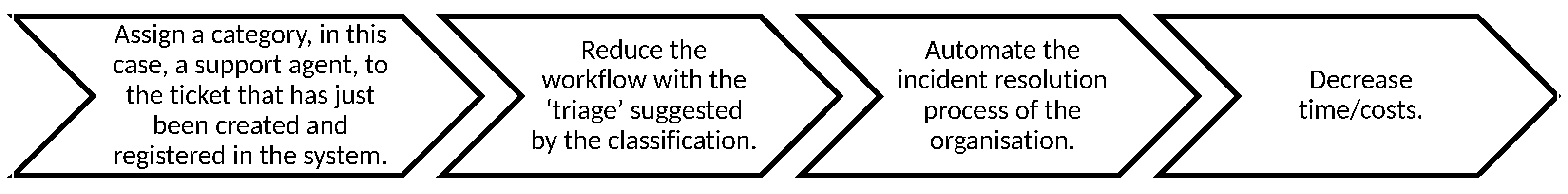
1.1. Problem Definition
1.2. Objectives
1.3. Methodologies
1.4. Document Structure
2. Literature Review
2.1. Information Technology Service Management
2.2. Incident Management Process
2.3. Text Mining
- Vector text 1 = [111100000]
- Vector text 2 = [110011111].
2.4. Machine Learning
Evaluation Metrics
- True Positives (VP)—the algorithm predicts 1 where it should predict 1.
- False Positives (FP)—the algorithm predicts 1 where it should predict 0.
- True Negatives (VN)—the algorithm predicts 0 where it should predict 0.
- False negatives (FN)—the algorithm predict 0 where it should predict 1.
- Acuity/Accuracy—used to measure the proportion of correct predictions over the total number of instances assessed.
- Precision/Precision—used to measure positive patterns predicted correctly from the total of patterns predicted in a positive class.
- Sensitivity/Recall—used to measure the fraction of positive patterns that are correctly classified.
- Averaged Precision—this metric calculates the average precision per class.
- Averaged Recall—this metric calculates the average recall per class.
- Averaged F-Measure—this metric calculates the average F-Measure by class.
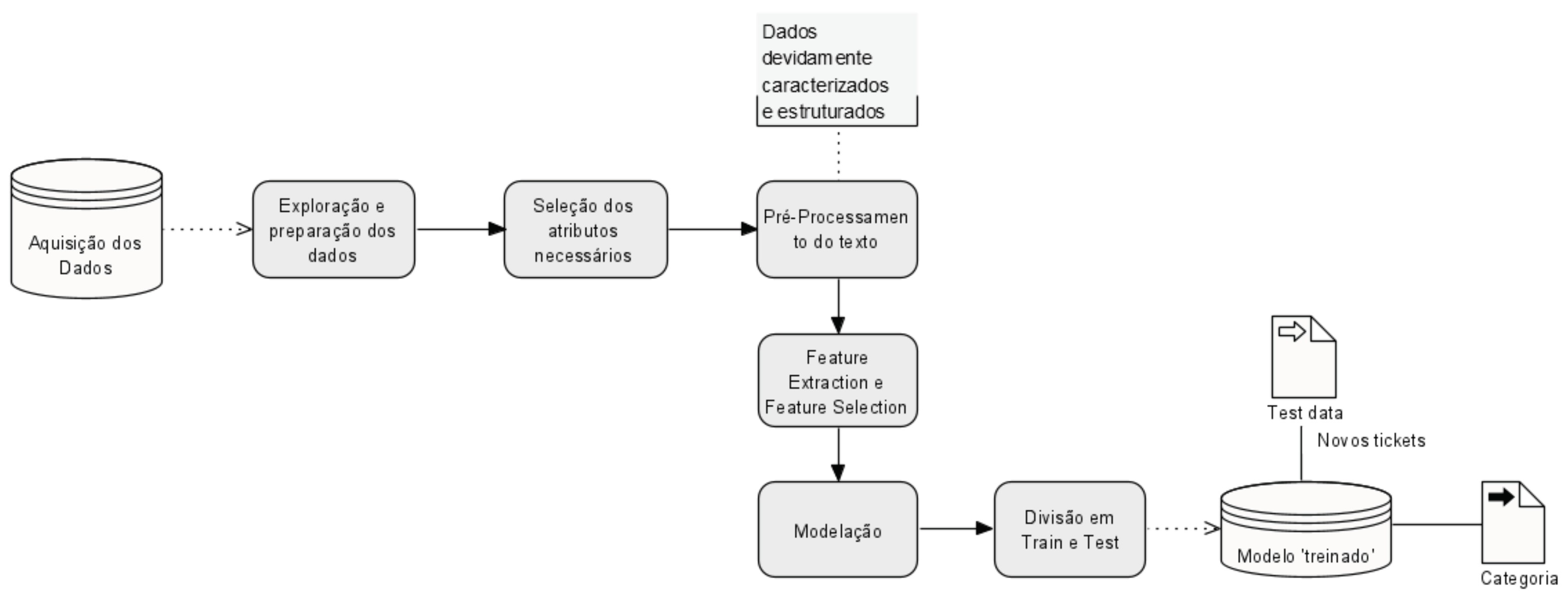
3. Text Classification Using CRISP-DM
3.1. Infrastructure
3.2. Business Understanding
3.3. Data Understanding and Preparation
3.3.1. Portuguese Language Dataset
3.3.2. Spanish Language Dataset
3.3.3. English Language Dataset
3.4. Data Processing
- Converge columns—concerns the union of the subject and note columns, transforming them into a new column called text.
- Removal of non-relevant technicians—the purpose of this is to remove the records attributed to agents not in the organization.
Word Processing
- Remove HTML tags—After analyzing the data and the specific ticket field, some HTML tags were removed.
- Convert to lowercase—All words were converted to lowercase.
- Remove special characters and punctuation—The removal was performed by replacing the unique characters and punctuation with blank spaces because, after removing these symbols, some words were combined.
- Removing blanks—This step is essential as the words are analyzed one by one; since a blank space can be considered a word and since it is not of significant importance, it is imperative to remove them.
- Remove stopwords—Stopwords are words that have no relevance to the intended analysis. These can be words like “de” (“of”), “o” (“the”) and “a” (“the”), among others (prepositions, articles), which occur very often in the descriptions of tickets. Therefore, they are removed.
- Stemming—This refers to reducing a word to its root. In the case of the word “amigo” (male friend), it would be reduced to “amig”. So, it fits “amigo” (male friend), “amiga” (female friend) and other words of the same family.
- Tokenization—This refers to the phase of dividing a text into a set of tokens; in this case, each word in that text would represent a token.
- TfidfVectorizer—All readers are converted to an array of features. What differentiates this process from CountVectorizer is that this last considers the number of times a word occurs in a document. In contrast, TfidfVectorizer considers the available weight in a document. By counting the occurrences of a word in a document, the importance of each word is calculated. Thus, it is convenient to detail the parameters defined in the specified method, sklearn.featurextraction.text.TfidfVectorizer:
- –
- underline_tf: This causes a logarithmic increase in the score compared to the frequency of a specific term. It arises in the problem in which, for example, there are 15 occurrences of a word in a text, but that does not mean that they are more critical than 1 occurrence of that term. In this case, this parameter is set to True.
- –
- min_df: When building a vocabulary, terms that have a strictly below the given limit are ignored. In this case, this parameter is provided a value of 5. This is because a word needs to be considered in at least 5 textual descriptions of a ticket.
- –
- norm: To reduce bias in the length of the document, this standardization parameter is used. At the same time, the score of each term scales proportionately, based on the total score of that document.
- –
- ngram_range: This parameter represents the lower and upper limits of the value range n for different n-grams extracted from the text. The values of n to be used are between .
- –
- stopwords: Defined as Portuguese, Spanish, or English, depending on the dataset being processed.
3.5. Modeling
3.5.1. Feature Extraction and Feature Selection
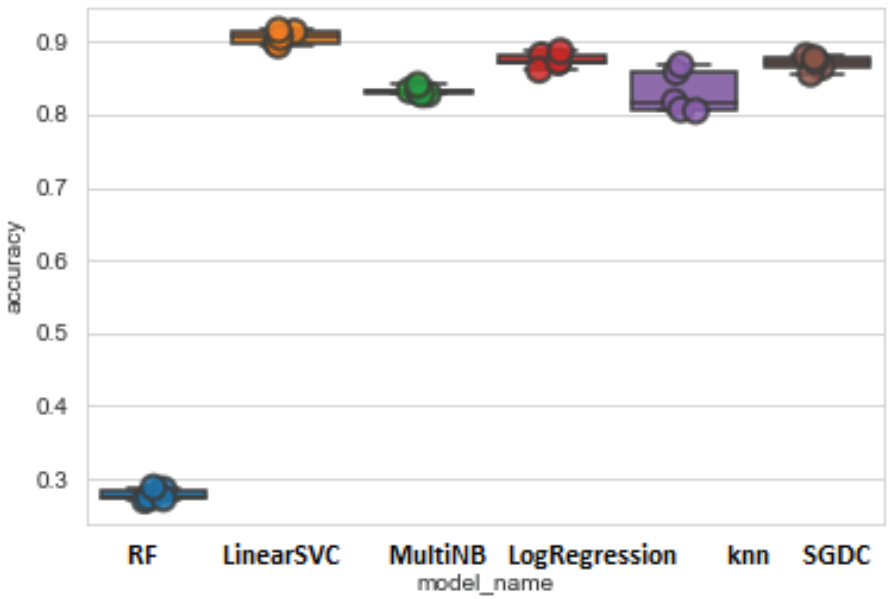
3.5.2. Selecting the Ideal Model
- Acuity/accuracy must be greater than 80%.
- Precision/precision must be greater than 75%.
- Sensitivity/recall must be greater than 80%.
- The error rate should not exceed the value of 20%.
3.6. Evaluation Methods
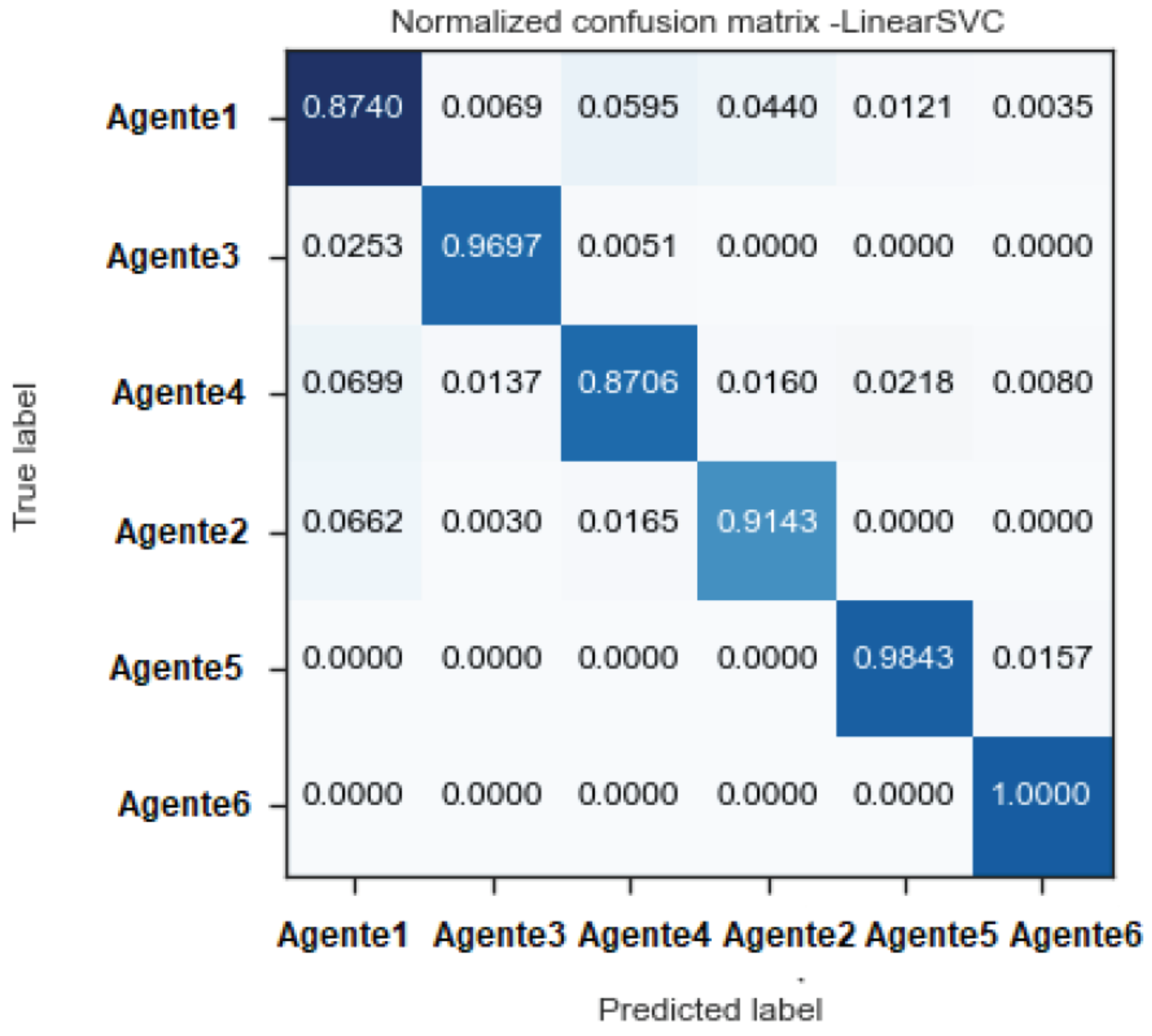
3.6.1. English Dataset
3.6.2. Making Predictions
3.6.3. Spanish and English Dataset
4. Discussion
4.1. English Dataset
4.2. Portuguese Dataset Comparison (C3) vs. Castilian vs. English
5. Conclusions
Author Contributions
Funding
Informed Consent Statement
Data Availability Statement
Conflicts of Interest
References
- Oliveira, D.F.; Brito, M.A. Development of Deep Learning Systems: A Data Science Project Approach. In Information Systems and Technologies; WorldCIST 2022. Lecture Notes in Networks and Systems; Rocha, A., Adeli, H., Dzemyda, G., Moreira, F., Eds.; Springer: Cham, Switzerland, 2022; Volume 469. [Google Scholar] [CrossRef]
- Hevner, A.R.; March, S.T.; Park, J.; Ram, S. Two Paradigms on Research Essay Design Science in Information Systems Research. MIS Q. 2004, 28, 75–79. [Google Scholar] [CrossRef]
- Ferreira, M.C. Incident Routing: Text Classification, Feature Selection, Imbalanced Datasets, and Concept Drift In Incident Ticket Management. Master’s Thesis, Universidade Federal do Rio de Janeiro, Rio de Janeiro, Brazil, 2017. [Google Scholar]
- Iden, J.; Eikebrokk, T.R. Implementing IT Service Management: A systematic literature review. Int. J. Inf. Manag. 2013, 33, 512–523. [Google Scholar] [CrossRef]
- Shahsavarani, N.; Ji, S. Research in Information Technology Service Management (ITSM): Theoretical Foundation and Research Topic Perspectives. CONF-IRM Proc. 2011, 30, 1–17. [Google Scholar]
- Tang, X.; Todo, Y. A Study of Service Desk Setup in Implementing IT Service Management in Enterprises. Technol. Investig. 2013, 4, 190–196. [Google Scholar] [CrossRef]
- Silva, S.A.T.D. Automatization of Incident Categorization. Ph.D. Thesis, University Institute of Lisbon, Lisbon, Portugal, 2018. [Google Scholar]
- Gulo, C.A.; Rúbio, T.R.; Tabassum, S.; Prado, S.G. Mining scientific articles powered by machine learning techniques. Open Access Ser. Inform. 2015, 49, 21–28. [Google Scholar] [CrossRef]
- Hass, N.; Hendrix, G.; Hobbs, J.; Moore, R.; Robinson, J.; Rosenschein, S.; Moore, R.; Robinson, J.; Rosenschein, S. DIALOGIC: A Core Natural-Language Processing System. In Proceedings of the 9th Conference on Computational Linguistics, Prague, Czech Republic, 5–10 July 1982. [Google Scholar] [CrossRef][Green Version]
- Forman, G. An Extensive Empirical Study of Feature Selection Metrics for Text Classification. J. Mach. Learn. Res. 2002, 1, 1289–1305. [Google Scholar] [CrossRef]
- Bahassine, S.; Madani, A.; Al-Sarem, M.; Kissi, M. Feature selection using an improved Chi-square for Arabic text classification. J. King Saud Univ. Comput. Inf. Sci. 2020, 32, 225–231. [Google Scholar] [CrossRef]
- Hussein, E.; Aliwy, A. Improving Feature Selection Techniques for Text Classification Esraa Hussein Abdul Ameer Alzuabidi. Ph.D. Thesis, University of Kufa, Kufa, Iraq, 2018. [Google Scholar]
- Al-harbi, O. A Comparative Study of Feature Selection Methods for Dialectal Arabic Sentiment Classification Using Support Vector Machine. IJCSNS Int. J. Comput. Sci. Netw. Secur. 2019, 19, 167–176. [Google Scholar]
- Justicia De La Torre, C.; Martín-Bautista, M.J.; Síanchez, D.; Vila, M.A. Text mining: Intermediate forms for knowledge representation. In Proceedings of the 4th Conference of the European Society for Fuzzy Logic and Technology and 11th French Days on Fuzzy Logic and Applications, EUSFLAT-LFA 2005 Joint Conference, Warsaw, Poland, 1 December 2005; pp. 1082–1087. [Google Scholar]
- George, K.S.; Joseph, S. Text Classification by Augmenting Bag of Words (BOW) Representation with Co-occurrence Feature. IOSR J. Comput. Eng. 2014, 16, 34–38. [Google Scholar] [CrossRef]
- Langley, P.; Carbonell, J.G. Approaches to machine learning. J. Am. Soc. Inf. Sci. 1984, 35, 306–316. [Google Scholar] [CrossRef]
- Jurafsky, D.; Martin, J.H. Speech and language processing: An Introduction to Natural Language Processing, Computational Linguistics and Speech Recognition. Rev. Soc. Econ. 2018, 40, 76–78. [Google Scholar] [CrossRef]
- Vedala, D. Building a Classification Engine for Ticket Routing in IT Support Systems. Master’s Thesis, Aalto University, Espoo, Finland, 2018. [Google Scholar]
- Hastie, T.; Tibshirani, R.; Friedman, J. The Elements of Statistical Learning, 2nd ed.; Springer: New York, NY, USA, 2009. [Google Scholar] [CrossRef]
- Hartmann, J.; Huppertz, J.; Schamp, C.; Heitmann, M. Comparing automated text classification methods. Int. J. Res. Mark. 2019, 36, 20–38. [Google Scholar] [CrossRef]
- Mao, W.; Wang, F.Y. Cultural Modeling for Behavior Analysis and Prediction. Adv. Intell. Secur. Inform. 2012, 91–102. [Google Scholar] [CrossRef]
- Misra, S.; Li, H. Noninvasive Fracture Characterization Based on the Classification of Sonic Wave Travel Times; Elsevier Inc.: Amsterdam, The Netherlands, 2020; pp. 243–287. [Google Scholar] [CrossRef]
- Belgiu, M.; Drăgu, L. Random forest in remote sensing: A review of applications and future directions. ISPRS J. Photogramm. Remote Sens. 2016, 114, 24–31. [Google Scholar] [CrossRef]
- Maertens, R.; Long, A.S.; White, P.A. Performance of the InVitro TransgeneMutation Assay in MutaMouse FE1Cells: Evaluation of NineMisleading (“False”) Positive Chemicals. Environ. Mol. Mutagen. 2010, 405, 391–405. [Google Scholar] [CrossRef]
- Ruder, S. An overview of gradient descent optimization algorithms. arXiv 2016, arXiv:1609.04747. [Google Scholar]
- Hossin, M.; Sulaiman, M.N. A Review on Evaluation Metrics for Data Classification Evaluations. Int. J. Data Min. Knowl. Manag. Process 2015, 5, 1–11. [Google Scholar] [CrossRef]
- Meesad, P.; Boonrawd, P.; Nuipian, V. A Chi-Square-Test for Word Importance Differentiation in Text Classification Natural Language Processing Techniques and Application. View project Text Classification View project A Chi-Square-Test for Word Importance Differentiation in Text Classification. In Proceedings of the International Conference on Information and Electronics Engineering, Singapore, 6 January 2011. [Google Scholar]


| O “The” | Ticket | Foi “Was” | Fechado “Closed” | Está “It Is” | À “the” | Espera “Wait” | De “in” | Resolução “Resolution” | |
|---|---|---|---|---|---|---|---|---|---|
| Text 1 | 1 | 1 | 1 | 1 | 0 | 0 | 0 | 0 | 0 |
| Text 2 | 1 | 1 | 0 | 0 | 1 | 1 | 1 | 1 | 1 |
| Actual/Foreseen | 1 | 0 |
|---|---|---|
| 1 | True Positives TP | False Positives FP |
| 2 | False Negatives FN | True Negatives TN |
| CRISP-DM [1] | DSR [2] |
|---|---|
| 1. Business Understanding | 1. Problem Identification and Motivation |
| 2. Understanding the Data | 2. Definition of objectives |
| 3. Data Preparation | 3. Design and Development |
| 4. Modeling | 4. Demonstration |
| 5. Evaluation | 5. Evaluation |
| 6. Implementation | 6. Communication |
| Dataset by Language | Record Period | Number of Tickets Registered |
|---|---|---|
| Portuguese Dataset | 12 March 2018–12 February 2020 | 4881 |
| Spanish Dataset | 13 March 2018–12 February 2020 | 1620 |
| English Dataset | 4 May 2018–11 February 2020 | 930 |
| Total | 7431 | |
| Column | Type | Description |
|---|---|---|
| AgentName | string | Indicates the Information Agent to which the ticket was assigned |
| Text | string | The column derived from the junction of the subject and description columns. |
| Portuguese | Spanish | English | |
|---|---|---|---|
| “Agent 6” | 46,436 | 6012 | 0 |
| “Agent 3” | 107,396 | 21,360 | 5160 |
| “Agent 1” | 98,748 | 48,510 | 5160 |
| “Agent 7” | X | X | 21,845 |
| “Agent 5” | 48,114 | 11,360 | 492 |
| “Agent 2” | 63,357 | 20,330 | 4911 |
| “Agent 8” | X | X | 4625 |
| “Agent 2” | 67,898 | 29,997 | 7467 |
| Total | 431,969 | 137,569 | 50,539 |
| Category | Unigrams | Bigrams |
|---|---|---|
| “Agent 6” | “install” | “replace PC” |
| “project” | “I need to install” | |
| “Agent 3” | “bi” | “him him” |
| “sgcp” | “power bi” | |
| “Agent 1” | “crm” | “error, error” |
| “error” | “error crm” | |
| “Agent 5” | “blocked” | “blocked system” |
| “system” | “system account” | |
| “Agent 2” | “to set up” | “times ti” |
| “ti” | “collaborative portal” | |
| “Agent 4” | “polycom” | “confirm given” |
| “checklist” | “form checklist” |
| Scenario (C) | N-Gram Variation |
|---|---|
| C1 | Unigrams + Bigrams + Stopwords + Stemming–Oversampling |
| C2 | Oversampling + Unigrams + Bigrams + Stopwords + Stemming |
| C3 | Oversampling + Unigrams + Bigrams + Stopwords |
| C4 | Oversampling + Unigrams + Bigrams |
| C5 | Oversampling + Stopwords + Unigrams |
| C6 | Oversampling + Stopwords + Bigrams |
| Algorithm | Settings | Value |
|---|---|---|
| Random Forest | N_estimators | 200 |
| Criterion | gini | |
| max_depth | 3 | |
| random_state | 0 | |
| LinearSVC | loss | squared_hinge |
| multi_class | ovr | |
| max_iter | 1000 | |
| Kernel | rbf | |
| Multinomial Naive Bayes | Alpha | 1.0 |
| Fit_prior | true | |
| Class_prior | None | |
| Logistic Regression | random_state | 0 |
| penalty | l2 | |
| max_iter | 200 | |
| KNN | n_neighbors | 5 |
| weights | Uniform | |
| SGDC | max_iter | 100 |
| penalty | l2 | |
| Loss | squared_hinge |
| Average Acuity | Standard Deviation | |||||||||||
|---|---|---|---|---|---|---|---|---|---|---|---|---|
| Algorithm Scenario | C1 | C2 | C3 | C4 | C5 | C6 | C1 | C2 | C3 | C4 | C5 | C6 |
| KNN | 58.21% | 81.5% | 81.26% | 81.16% | 80.85% | 83.11% | 4.67 | 6.92 | 6.99 | 7.3 | 5.99 | 2.98 |
| LinearSVC | 65.09% | 97.35% | 97.51% | 97.6% | 94.17% | 90.57% | 4.01 | 0.41 | 0.98 | 0.35 | 0.65 | 0.91 |
| LR | 65.73% | 91.73% | 92.21% | 92.55% | 88.95% | 87.48% | 4.64 | 0.49 | 0.52 | 0.45 | 0.55 | 0.98 |
| MNB | 63.35% | 86.48% | 87.35% | 87.63% | 82.44% | 83.21% | 3.7 | 0.36 | 0.39 | 0.38 | 0.78 | 0.52 |
| RF | 40.51% | 29.36% | 29.94% | 29.96% | 30.51% | 27.81% | 2.8 | 1.05 | 1.47 | 1.28 | 1.23 | 0.8 |
| SGDC | 65.32% | 92.74% | 93.14% | 93.46% | 89.18% | 87.21% | 4.56 | 0.61 | 0.46 | 0.36 | 0.59 | 1.04 |
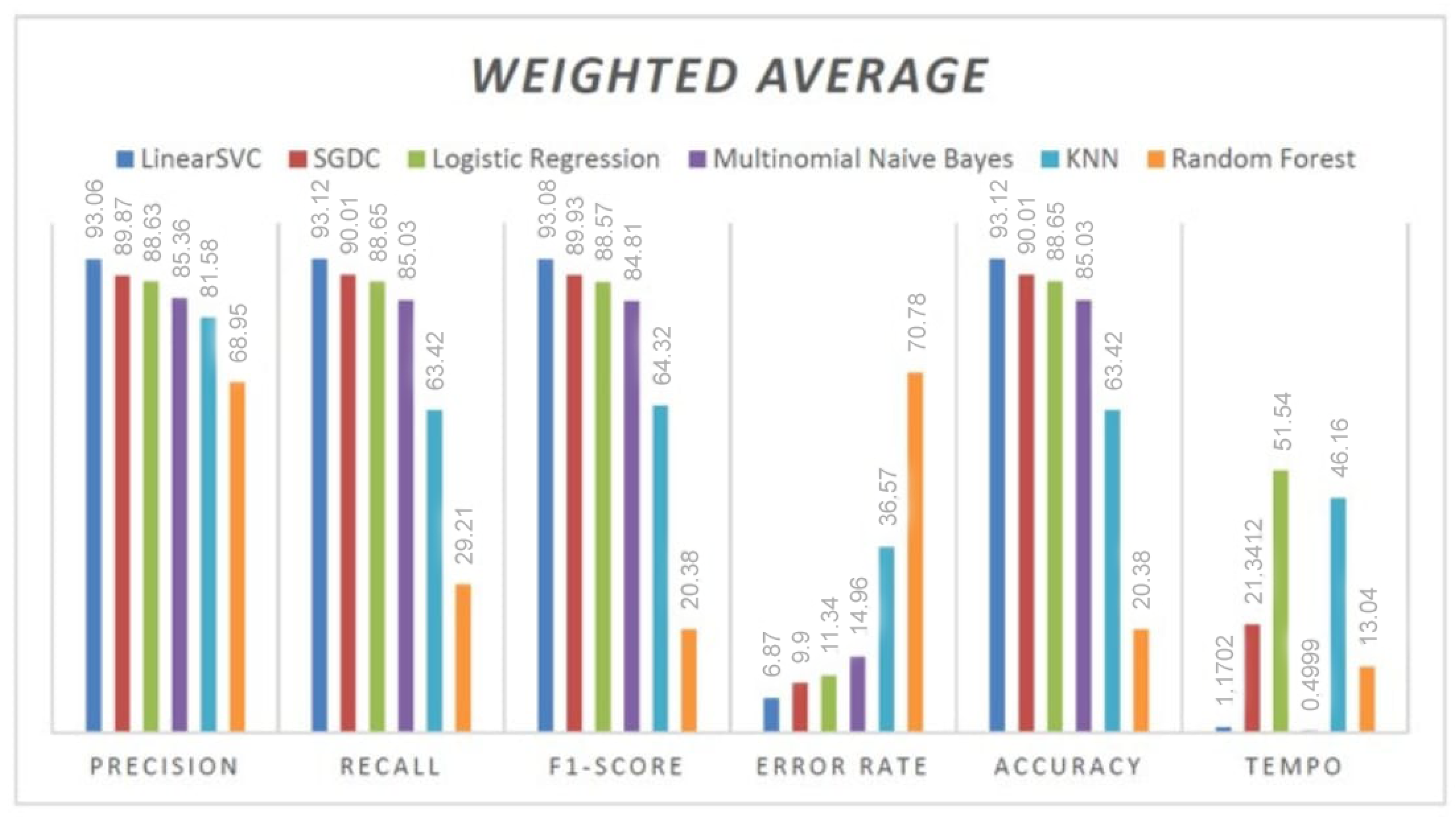
| Precision | Sensitivity | F1-Score | Support | Error | Acuity | Time(s) | |
|---|---|---|---|---|---|---|---|
| LinearSVC | 93.06% | 93.12% | 93.08% | 5137 | 6.87% | 93.12% | 1.1702 |
| LR | 88.63% | 88.65% | 88.57% | 5137 | 11.34% | 88.65% | 51.54 |
| SGDC | 89.87% | 90.01% | 89.93% | 5137 | 9.9% | 90.01% | 21.3412 |
| MNB | 85.36% | 85.03% | 84.81% | 5137 | 14.96% | 85.03% | 0.4999 |
| KNN | 81.58% | 63.42% | 64.32% | 5137 | 36.57% | 63.42% | 46.16 |
| RF | 68.95% | 29.21% | 20.38% | 5137 | 70.78% | 29.21% | 13.04 |
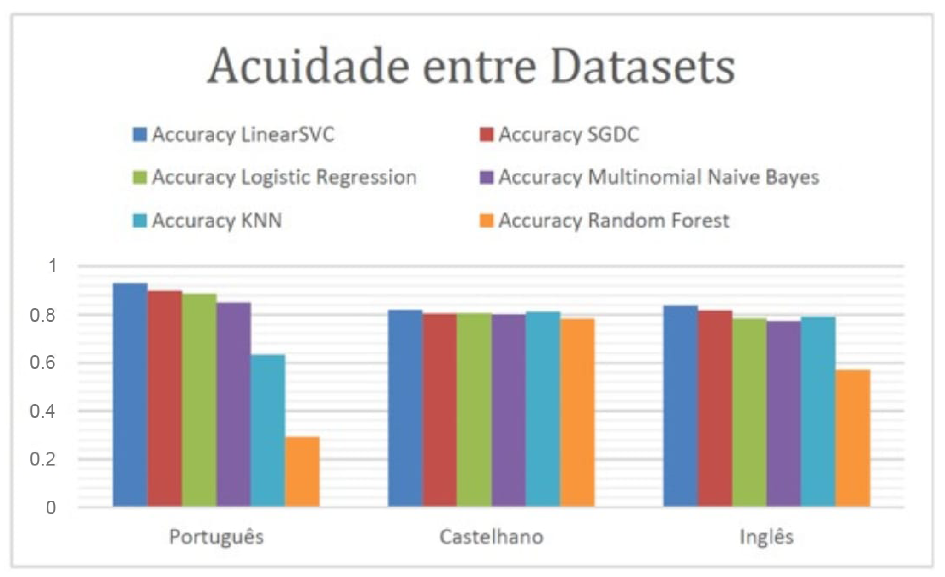
| Metric | LinearSVC | MNB | LR | RF | KNN | SGDC | |
|---|---|---|---|---|---|---|---|
| Spanish | Average Acuity | 82.67% | 81.04% | 82.1% | 78.97% | 80.1% | 81.35% |
| Standard deviation | 1 | 1.4 | 1.4 | 0.03 | 1.1 | 1.9 | |
| English | Average Acuity | 80.16% | 78.39% | 78.51% | 57.56% | 77.09% | 77.19% |
| Standard deviation | 4.65 | 2.68 | 3.25 | 0.51 | 77.19 | 3.5 |
| Algorithm | Precision | Sensitivity | F1-score | Acuity | Error Rate | Time(s) | |
|---|---|---|---|---|---|---|---|
| Spanish | LinearSVC | 79.17% | 81.93% | 78.77% | 81.93% | 18.06% | 2.19 |
| MNB | 71.20% | 80.03% | 75.26% | 80.03% | 19.96% | 0.69 | |
| LR | 71.30% | 80.6% | 74.71% | 80.6% | 19.39% | 29.98 | |
| RF | 61.35% | 78.32% | 68.8% | 78.32% | 21.67% | 53.36 | |
| KNN | 78.99% | 81.17% | 76.81% | 81.17% | 18.82% | 28.68 | |
| SGDC | 77.75% | 80.41% | 78.76% | 80.41% | 19.58% | 24.88 | |
| English | LinearSVC | 82.12 | 83.72 | 82.26 | 83.72 | 16.27 | 1.19 |
| MNB | 78.29 | 77.4 | 74.17 | 77.4 | 22.59 | 0.79 | |
| LR | 79.10 | 78.4 | 75.52 | 78.4 | 21.59 | 17.68 | |
| RF | 41.77 | 57.14 | 42.76 | 57.14 | 42.85 | 46.47 | |
| KNN | 77.60 | 79.06 | 78.17 | 79.06 | 20.93 | 8.7 | |
| SGDC | 80.46 | 81.72 | 81.03 | 81.72 | 18.27 | 10.2 |
| Category | Metric | LinearSVC (%) | LR (%) | RF (%) | MNB (%) | KNN (%) | SGDC (%) |
|---|---|---|---|---|---|---|---|
| “Agent1” | Precision | 89.01 | 80.69 | 24.17 | 73.4 | 82.35 | 86.2 |
| Sensitivity | 87.4 | 82.57 | 99.65 | 82.13 | 31.4 | 80.32 | |
| F1-Score | 88.2 | 81.62 | 38.9 | 77.52 | 45.47 | 83.16 | |
| Support | 1159 | ||||||
| “Agent2” | Precision | 90.34 | 88.31 | 0 | 90.94 | 27.33 | 86.72 |
| Sensitivity | 91.42 | 81.8 | 0 | 67.96 | 93.38 | 86.46 | |
| F1-Score | 90.88 | 84.93 | 0 | 77.7 | 42.28 | 86.59 | |
| Support | 665 | ||||||
| “Agent3” | Precision | 97.21 | 95.21 | 93.56 | 91.07 | 92.2 | 93.25 |
| Sensitivity | 96.96 | 90.53 | 23.86 | 87.62 | 50.75 | 95.95 | |
| F1-Score | 97.09 | 92.81 | 38.02 | 89.31 | 65.47 | 94.58 | |
| Support | 792 | ||||||
| “Agent4” | Precision | 90.04 | 84.8 | 100 | 81.71 | 85.66 | 84.89 |
| Sensitivity | 87.05 | 80.52 | 5.15 | 73.19 | 29.43 | 84.3 | |
| F1-Score | 88.52 | 82.6 | 9.8 | 77.22 | 43.81 | 84.59 | |
| Support | 873 | ||||||
| “Agent5” | Precision | 96.1 | 90.6 | 100 | 88.52 | 94.52 | 93.24 |
| Sensitivity | 98.43 | 99.03 | 7.6 | 98.79 | 95.89 | 98.43 | |
| F1-Score | 97.25 | 94.63 | 14.14 | 93.37 | 95.2 | 95.76 | |
| Support | 828 | ||||||
| “Agent6” | Precision | 97.15 | 95.87 | 100 | 92.91 | 96.81 | 97.01 |
| Sensitivity | 100 | 99.14 | 5.9 | 99.14 | 100 | 99.14 | |
| F1-Score | 98.55 | 97.48 | 11.27 | 95.92 | 98.38 | 98.07 | |
| Support | 820 | ||||||
| Acuidade | 93.12 | 88.65 | 29.21 | 85.03 | 63.42 | 90.13 | |
| Possible Incident Ticket | Expected Computer Agent |
|---|---|
| “I need you to install a printer for me and replace the toner.” | “Agent 6” |
| “Power BI on my pc doesn’t work” | “Agent 3” |
| “I need you to cancel an order in SAP.” | “Agent 1” |
| “I need to recover a file that I ended up not saving to the PDM” | “Agent 4” |
| “What about the employee portal?” | “Agent 2” |
| “My account is blocked.” | “Agent 6” |
Publisher’s Note: MDPI stays neutral with regard to jurisdictional claims in published maps and institutional affiliations. |
© 2022 by the authors. Licensee MDPI, Basel, Switzerland. This article is an open access article distributed under the terms and conditions of the Creative Commons Attribution (CC BY) license (https://creativecommons.org/licenses/by/4.0/).
Share and Cite
Oliveira, D.F.; Nogueira, A.S.; Brito, M.A. Performance Comparison of Machine Learning Algorithms in Classifying Information Technologies Incident Tickets. AI 2022, 3, 601-622. https://doi.org/10.3390/ai3030035
Oliveira DF, Nogueira AS, Brito MA. Performance Comparison of Machine Learning Algorithms in Classifying Information Technologies Incident Tickets. AI. 2022; 3(3):601-622. https://doi.org/10.3390/ai3030035
Chicago/Turabian StyleOliveira, Domingos F., Afonso S. Nogueira, and Miguel A. Brito. 2022. "Performance Comparison of Machine Learning Algorithms in Classifying Information Technologies Incident Tickets" AI 3, no. 3: 601-622. https://doi.org/10.3390/ai3030035
APA StyleOliveira, D. F., Nogueira, A. S., & Brito, M. A. (2022). Performance Comparison of Machine Learning Algorithms in Classifying Information Technologies Incident Tickets. AI, 3(3), 601-622. https://doi.org/10.3390/ai3030035