Article

MSG-GAN-SD: A Multi-Scale Gradients GAN for Statistical Downscaling of 2-Meter Temperature over the EURO-CORDEX Domain

by
Gabriele Accarino
1,2,†,
Marco Chiarelli
1,2,†,
Francesco Immorlano
1,3,†,
Valeria Aloisi
1,3,
Andrea Gatto
1,3 and
Giovanni Aloisio
1,3,*
1
Euro-Mediterranean Center on Climate Change (CMCC) Foundation, Via Augusto Imperatore, 16, 73100 Lecce, Italy
2
Department of Biological and Environmental Sciences and Technologies, University of Salento, Via Provinciale Lecce-Monteroni, 73100 Lecce, Italy
3
Department of Innovation Engineering, University of Salento, Via Provinciale Lecce-Monteroni, 73100 Lecce, Italy
*
Author to whom correspondence should be addressed.
These authors contributed equally to this work.
AI 2021, 2(4), 600-620; https://doi.org/10.3390/ai2040036
Submission received: 27 September 2021 / Revised: 10 November 2021 / Accepted: 15 November 2021 / Published: 19 November 2021

Abstract

:
One of the most important open challenges in climate science is downscaling. It is a procedure that allows making predictions at local scales, starting from climatic field information available at large scale. Recent advances in deep learning provide new insights and modeling solutions to tackle downscaling-related tasks by automatically learning the coarse-to-fine grained resolution mapping. In particular, deep learning models designed for super-resolution problems in computer vision can be exploited because of the similarity between images and climatic fields maps. For this reason, a new architecture tailored for statistical downscaling (SD), named MSG-GAN-SD, has been developed, allowing interpretability and good stability during training, due to multi-scale gradient information. The proposed architecture, based on a Generative Adversarial Network (GAN), was applied to downscale ERA-Interim 2-m temperature fields, from 83.25 to 13.87 km resolution, covering the EURO-CORDEX domain within the 1979–2018 period. The training process involves seasonal and monthly dataset arrangements, in addition to different training strategies, leading to several models. Furthermore, a model selection framework is introduced in order to mathematically select the best models during the training. The selected models were then tested on the 2015–2018 period using several metrics to identify the best training strategy and dataset arrangement, which finally produced several evaluation maps. This work is the first attempt to use the MSG-GAN architecture for statistical downscaling. The achieved results demonstrate that the models trained on seasonal datasets performed better than those trained on monthly datasets. This study presents an accurate and cost-effective solution that is able to perform downscaling of 2 m temperature climatic maps.

1. Introduction

Downscaling is a procedure that allows making predictions at local scales, starting from climatic field information available at large scale. In climate science, a well-established representation of climatic fields involves the use of multi-dimensional structures (i.e., 2D, 3D or even 4D if the time dimension is considered) that can be treated as single images or image sequences [1,2,3,4,5]. Therefore, the grid points in a climatic map can be represented as image pixels. This is the reason why the downscaling problem is closely related to the super-resolution (SR) problem in computer vision and image processing, corresponding to the enhancement of the spatial resolution of an image beyond its original resolution [6,7,8,9,10,11]. Thus, a prior extensive knowledge about the structure of the images at the target finer resolution is critical for SR models, and enables them to generate upsampled images that are coherent with the input data [10]. The task of producing a super-resolution image (from now on called an HR image), starting from its lower resolution counterpart (from now on called an LR image), is recognized in the literature as single-image super resolution (SISR) [10]. This problem is generally ill-posed because it does not have a unique solution, as many different HR images can be generated starting from the same LR image [11]. In fact, the upsampling procedure involves the synthesis of artificial information which serves to scale-up the image towards the target resolution. (In this scenario, the terminology may lead to confusion as the terms “upsampling” and “upscaling” are both used in computer vision to indicate the process of increasing the number of pixels in an image, whereas the term “downsampling” indicates the inverse process. In climate science, the term “downscaling” refers to the generation of maps with a finer resolution (i.e., with a higher number of grid points), starting from their coarser resolution. This is due to the fact that the finer resolution maps, generated through a downscaling process, will consist of grid points with a smaller horizontal resolution.). The need for downscaling is generally motivated by the typically unsatisfactory coarse resolution of global climate models (GCMs). Although these models are used for a better understanding of climate change at global and up to continental scales, and provide information for a large number of climatic fields, they are not able to resolve processes that manifest at regional and local scales, whose dynamics are often critical for assessing the impacts of a changing climate on society [3,12]. Downscaling can be carried out through two classes of techniques: dynamical and statistical. The former is performed through a physics-based model, namely a regional climate model (RCM), that involves a set of physical equations for modeling different components of the climatic system and their interactions. The physical laws are numerically solved in order to simulate the outcomes for a series of different climatic fields at a finer resolution. The statistical techniques, which are typically more accurate than the model’s raw output [13], involve the learning of empirical statistical relationships between coarse GCM outputs and HR products [3,4,12,14]. Inspired by the work presented in [15], a multi-scale deep architecture was developed for downscaling the 2-m temperature (T2M), from 0.75° × 0.75° up to 0.125° × 0.125° of spatial resolution, in the past 40 years (1979–2018), over the European domain by exploiting Era-Interim analysis data [16]. The aim was to provide a novel deep learning-based solution to the downscaling task, as an alternative to traditional dynamical and statistical techniques. This was also motivated by the cost-effectiveness of deep learning models that, once trained, provide outcomes through a limited amount of computing resources and execution time. The proposed architecture, named Multi-Scale Gradients GAN for Statistical Downscaling (from now on called MSG-GAN-SD), features a Generative Adversarial Neural Network (GAN) composed of Generator (from now on called G) and Discriminator (from now on called D) networks, that are both convolutional and set to work at multiple scales. Each of these networks is made up of several blocks exploiting multiple versions of the same image at different resolutions, depending on the specific scale. This allows the propagation of gradients coming from multiple scales during the training phase. As opposed to other similar works based on statistical downscaling of climatic fields, low-resolution T2M heatmaps were not artificially downsampled from the high-resolution counterpart, because images were directly gathered at low and high resolutions. Furthermore, the present study introduced an experimental multi-stage framework for evaluation purposes.

Related Work

According to [17], statistical downscaling is classified into three sub-categories: regression-based, weather classification-based, and weather generators-based approaches. Concerning regression-based approaches, several attempts at downscaling a variety of climatic fields—mainly temperature, precipitation and wind fields—have been proposed in recent years. Machine learning (ML) techniques have been widely adopted for downscaling. In particular, the LASSO regression was used in [18] for downscaling precipitation, whereas genetic programming (GP) was exploited in [19] and [20] for downscaling precipitation and temperature, and daily minimum and maximum temperature, respectively. Moreover, the random forest (RF) was used in [21] for land surface temperature, whereas a novel hybrid dynamical-statistical approach was presented in [22] focusing on the resolution of fine-scale rainfalls with lower computational costs, through a combination of dynamical and statistical downscaling. Artificial Neural Networks (ANNs) have been used in [23] to perform precipitation downscaling, applying a further residual correction method based on Particle Swarm Optimization (PSO), an Imperialist Competitive Algorithm (ICA), and a Genetic Algorithm (GA). Furthermore, a Back-Propagation Neural Network (BPNN) and Support Vector Machine (SVM) fusion approach was adopted in [24] to downscale precipitation. Several works moved towards deep architectures in the context of Deep Learning (DL), especially concerning Long-Short Term Memory (LSTM) networks, Convolutional Neural Networks (CNNs) and Generative Adversarial Networks (GANs). Since their introduction presented in [25], LSTMs have been proven to be suitable for recovering and bridging information arbitrarily far in time, while avoiding the vanishing gradient problem. LSTMs have also been widely adopted for time-series related problems and, in the context of climate downscaling, for statistical downscaling of precipitation [26] and rainfall forecasting [27] in combination with Feed Forward Neural Networks (FFNNs). Convolutional Neural Networks (CNNs), due to their ability to deal with spatio-temporal multi-dimensional structures, have been demonstrated to be particularly suitable for accomplishing SR tasks. Several attempts to use deeper architectures have been proposed [28,29,30,31,32,33] for the extraction of high-level image characteristics and the downscaling of climatic fields. A deep neural network based on a CNN and a LSTM recurrent module was proposed in [34] to estimate precipitation based on well-resolved atmospheric dynamical fields. A novel architecture, named DeepSD, based on the super resolution framework, was presented in [1,2] for downscaling precipitation fields, and a CNN-based approach was proposed in [13] as an alternative solution to the existing precipitation-related parameterization schemes for the numerical precipitation estimation. A CNN model for downscaling the occurrence of precipitation was also proposed in [3], whereas different configurations of CNN were adopted in [35] to downscale daily temperature and precipitation over China. A competitive DL framework based on a CNN was presented in [36] for downscaling temperature and precipitation, and it performed particularly well in generating spatio-temporal details at very fine-grid scales. A U-Net-type CNN was also used in [37] to learn a one-to-one mapping of low-resolution (input) to high-resolution (output) wind fields simulations data, and a conditional variational autoencoder (based on CNN) was exploited for learning the conditional distributions from data, assessing multimodalities and uncertainties. A CNN was adopted in [38] to perform smart dynamical downscaling (SDD) for extreme precipitation events, whereas a surrogate model, based on a Deep CNN (DCNN), was evaluated in [39] for surface temperature, and was found to estimate image details that were not retained in the inputs. Recently, remarkable results were reported in several studies exploiting GANs for SR tasks in climate science. An Enhanced Super-Resolution GAN (ESRGAN) [40] was adopted and presented in [41] to downscale wind speeds from a coarse grid, capturing high frequency power spectra and high order statistics in the dataset, thus generating images of superior visual quality compared to the SR-CNN. A novel method (ClimAlign) was introduced in [42] for unsupervised, generative downscaling of temperature and precipitation based on normalizing flows for variational inference. Further works [4,43,44,45,46,47,48,49,50] opted for downscaling based on ML and DL, and they helped assess both strengths and weaknesses of such methods. The results reported in these studies show that downscaling models based on ML allow better performance with respect to the other statistical approaches presented in [51,52,53].

2. Materials and Methods

2.1. Data

The proposed work aimed at downscaling 2-meter temperature over the EURO-CORDEX domain [54], by learning a statistical relationship between HR images and their LR counterparts, each one representing a temperature map. Analysis data was gathered in NetCDF4 format [55] from the COPERNICUS ERA-Interim global atmospheric reanalysis dataset [16], and treated as images throughout the various experiments, according to the SISR framework. All the background information can be found in [56]. From the global domain, the EURO-CORDEX subdomain was selected for both resolutions, from −48.5° E to 69.75° E of longitude and from 73.9° N to 20.15° N of latitude. The horizontal resolutions of HR and LR images are about 13.87 km (0.125° × 0.125°) and 83.25 km (0.75° × 0.75°) respectively, whereas the related images sizes are 431 × 947 and 72 × 158 pixels. The data covers a temporal range from January 1979 to December 2018 (40 years) and is made up of 6-hourly samples. Thus, each day of a year consists of four samples, at 00:00, 06:00, 12:00 and 18:00, respectively.

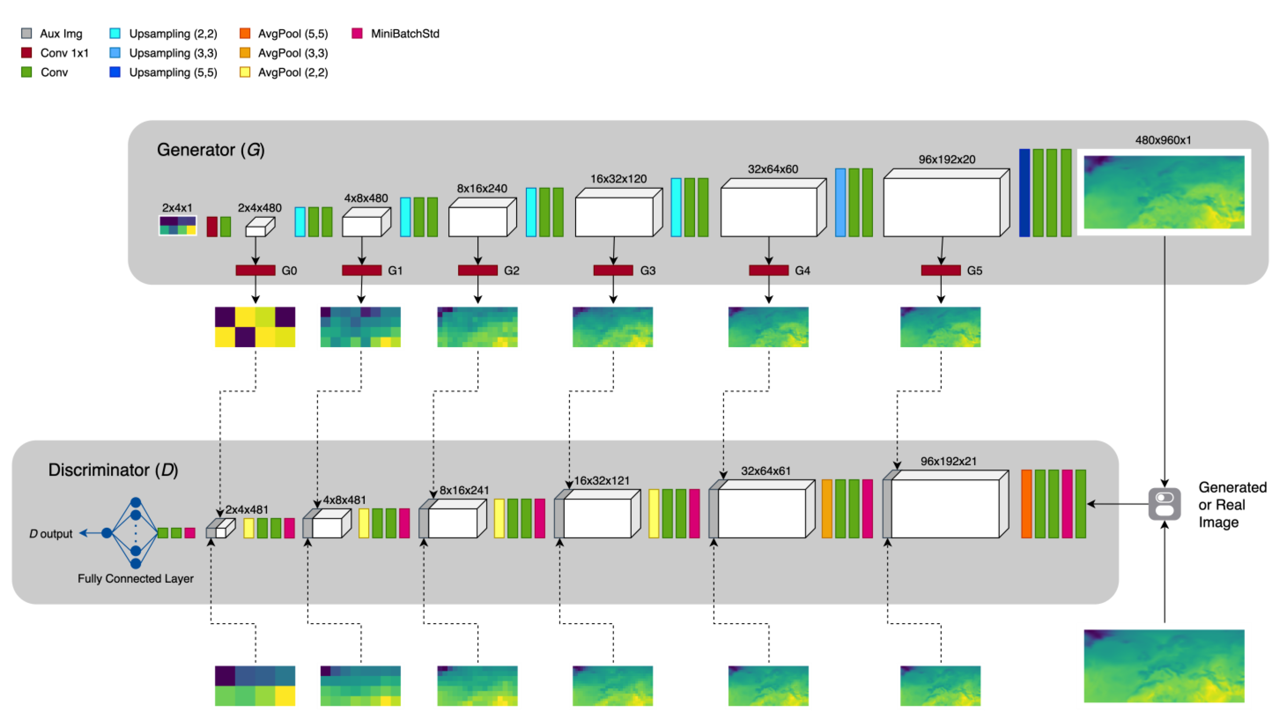
2.2. The Architecture: Multi-Scale Gradients GAN for Statistical Downscaling

The proposed Multi-Scale Gradients GAN architecture for statistical downscaling (MSG-GAN-SD, reported in Figure 1) is based on the fusion of two frameworks, that is, the super resolution GAN defined in [57] and the Multi-Scale Gradients GAN proposed in [15]. The multi-scale framework in [15] was considered in order to speed up both the development and the tuning of the model, overcoming the difficulties of a conventional GAN caused by its training instabilities. The nature of the statistical downscaling task required the employment of a SR architecture [57], in which a LR version of the HR image (target) is used to feed G, instead of the random latent vector proposed in [58]. In [15], two implementations of the MSG framework were described: the MSG-ProGAN and the MSG-StyleGAN. They share the same architectural structure (layers) for G, but differ for D layers and the loss functions used. The present study selected the MSG-ProGAN [15] as the baseline architecture and used the Wasserstein GAN with Gradient Penalty (WGAN-GP) loss function [59]. Both G and D retain the ascending and descending complexity pattern of the MSG-ProGAN layers. At the early stages of development, the architectures reported in Table A1 and Table A2 of Appendix A were adopted for G and D, respectively, in order to match the 2 × 4 low-resolution and 480 × 960 high-resolution padded images. Starting from a 2 × 4 input image, obtained by progressively undersampling the original LR image (see Section 2.3), G produces upsampled images at finer scales. Specifically, at the end of each block of G, an image is generated at the associated scale (see G 0 G 5 blocks in Table A1). The generated images have the property of being intelligible (once denormalized), thus representing the downscaled temperature map at a particular resolution. When discriminating the generated (fake) samples, images produced by G 0 G 5 are to be considered as auxiliary images that are further fed to the blocks of D matching the corresponding resolutions. By comparison, when D discriminates real samples, D blocks are additionally fed with the correspondingly downsampled version of higher resolution real images. In both cases, the auxiliary images in a certain block of D are concatenated with the activation volume coming from the preceding block, by means of a simple combine function. After each convolution, a Leaky ReLU (LReLU) with α = 0.2 was used in order to keep positive values unchanged and lower the negative values. In addition, only for G, the PixelNormalization scheme [60] was used after each activated convolution, in order to make convergence faster and prevent signals escalation. A MinBatchStdDev [61,62] layer was used at the beginning of each block of D to obtain statistics about the batch formed by the previous activation volume and the auxiliary image along with the different scales, thus improving sample diversity [15]. Concerning the WGAN-GP loss, because D is a function of multi-scale input images produced by G or the corresponding ground truth HR images at different resolutions, the gradient penalty was modified to be the average of the penalties over each input. This dependence makes the multi-scale gradients able to flow between intermediate layers of both D and G [15].

2.3. Data Preprocessing

In order to match architectural needs, HR images were artificially padded through edge-padding before training and test phases, going from 431 × 947 to 480 × 960 pixels. Edge-padding consists of adding a certain number of rows and columns at the image edges, by replicating the pixel values at the edges. Subsequently, starting from the 480 × 960 resolution, different scale versions of the padded images were progressively generated by means of the bilinear interpolation undersampling technique: 96 × 192, 32 × 64, 16 × 32, 8 × 16, 4 × 8, and 2 × 4. The edge-padding was also used for LR images, going from 72 × 158 to 80 × 160 pixels. Subsequently, the bilinear interpolation technique was applied to undersample padded LR images from 80 × 160 to 2 × 4 grid points, passing through the following intermediate resolutions: 40 × 80, 20 × 40, 10 × 20. The progressive undersampling procedure allows losing as little information as possible. Additionally, each resolution was chosen to maintain the same proportionality between rows (latitude) and columns (longitude), in order to satisfy the multi-scale framework requirements. Data was partitioned into three non-overlapping subsets, namely training, validation and test sets, that correspond to 87.5% (1979–2013, 35 years), 2.5% (2014, 1 year) and 10% (2015–2018, 4 years) of the whole dataset, respectively. Both HR and 2 × 4 images were normalized in the range [−1, 1] by computing their own maximum and minimum on the training set, and then by scaling all images in the training, validation and test sets, accordingly. Furthermore, because D takes multiple images at different resolutions as input, and these images were constructed from the HR image by applying progressive downsampling, the intermediate scales were also normalized by using HR image extrema. The same procedure was also applied for normalizing 2 × 4 images to be fed to G. Once the output is produced by G, a denormalization of the HR images is required to get back to the original temperature values. Afterwards, both generated and real HR images in full resolution were processed in order to remove the edge-padding. As explained in Section 2.4, two dataset arrangements were derived: the monthly set-up, where data is organized in twelve subsets, each one referring to a particular month, across different years (e.g., January 1979, January 1980, …, January 2018); and the season-based set-up, where data is organized in four subsets, each one referring to a particular season across different years (e.g., DJF 1979, DJF 1980, …, DJF 2018). In the remainder of the manuscript, seasons are intended to be DJF (December–January–February), MAM (March–April–May), JJA (June–July–August) and SON (September–October–November), according to the climate science scientific literature.

2.4. Experimental Setup

Experiments were carried out exploiting the Marconi100 GPU cluster hosted by CINECA [63]. The HPC system is based on the IBM Power9 architecture with NVIDIA Volta GPUs. Specifically, each node hosts 2 × 16 cores IBM POWER9 AC922 at 3.1 GHz with 256 GB/node of RAM memory and 4 × NVIDIA Volta V100 GPUs per node, Nvlink 2.0, 16 GB [64]. Regarding the software adopted for our implementation, both architecture and training/test control flows were written in Python v3.8.2 based on the Keras API v2.4.3 [65] and relying on the TensorFlow v2.2.0 [66] backend. Training was performed in a distributed fashion by means of the TensorFlow Distributed Training [67] and MirroredStrategy. The results of the present study were achieved by running the model on just one node of the Marconi100 cluster exploiting all 4 GPUs available.

2.4.1. Training Set Arrangements

Because the dataset consists of 40 years of data, two dataset arrangements were derived: (i) monthly, where the dataset was organized in twelve subsets, each having data referring to a particular month across different years (e.g., January 1979, January 1980, …, January 2018); and (ii) season-based, where the dataset was organized in four subsets, each having data referring to a particular season across different years (e.g., DJF 1979, DJF 1980, …, DJF 2018). Clearly, the seasonal arrangement dataset is three times bigger than the monthly dataset because the same number of years is considered. Training the model on month- and season-based arrangements of the same dataset allows gaining valuable insights into the ability of the MSG-GAN-SD to capture intra-monthly, intra-seasonal and/or inter-annual climatic dynamics [14]. In this manner, the models’ capability of capturing daily anomalies and extreme events is ensured, as reported in [12]. Consequently, a total of 12 monthly and 4 seasonal generator models were collected after the training phase. Therefore, during the inference phase, each monthly model was able to generate a downscaled T2M map for the corresponding month, whereas each seasonal model was able to provide maps for each month belonging to the corresponding season.

2.4.2. Training Configurations

In the literature, a well-known strategy for WGAN-GP framework is to make D able to learn more quickly, leading it to be more powerful than G at a particular training epoch. This is based on the intuition that, during the training phase, if D is sufficiently accurate in the discrimination task, then its gradients flowing back and the subsequent update of G weights allow an improvement of the generation task [59,68]. This strategy can be carried out in at least three ways: (i) raising D learning rates with respect to G; (ii) making D deeper, thus increasing its number of weights and enhancing its capacity; and (iii) using an imbalanced training, particularly suited for deep GANs. In this case, for each epoch, the Discriminator weights are updated more times with respect to those used for the Generator. The number of the discriminator updates is, from now on, referred to as DtrainUpdates. In the present study, a batch size of 64 and the RMSProp optimizer [69] with learning rates of 0.0003 and 0.0001 were used for G and D, respectively. However, because of memory issues, it was not possible to deepen D. Despite this, the discriminator was trained using three different update configurations (DtrainUpdates = 1, 2, 3 respectively). Therefore, a total of 48 models (12 monthly models × 3 DtrainUpdates + 4 seasonal models × 3 DtrainUpdates) were trained for 1000 epochs, saving them every 50 epochs.

2.4.3. The Validation Framework

The experimental workflow consisted of training the proposed architecture on the four climatological seasons (i.e., DJF, MMA, JJA, SON) and all twelve months, for all DtrainUpdates configurations (i.e., 1, 2, 3). The validation framework was based on three phases: (1) extraction of the best models through the minimization of a mathematical expression aiming to select the epoch in which the architecture performed better, by looking at training and cross-validation errors; (2) an evaluation procedure, which assessed the quality of the previously selected models by computing several metrics on the test set; and (3) a final test procedure, in which insightful climatological aggregated maps were created, using the previously selected best models.
(1)
Best Models Selection
For each seasons/DtrainUpdates and months/DtrainUpdates combination, it was necessary to select a model at the training epoch in which the network was sufficiently mature. This means that it well approximated the mapping between the ground truth and the generated distributions, without incurring a lack of generalization. Therefore, this epoch should be the point where the trade-off between underfitting and overfitting is reached. At the same time, accuracy and variety (or sample diversity) capabilities also need to be considered. In order to consider these factors during the training phase, different random batches of samples, coming from both training and validation sets, were monitored by computing the batch-averaged MSE between generated and real HR images, across scales. By using these variable batches, it was possible to check both the accuracy and the variety of the ongoing trained models at the same time. Ideally, the epoch at which the training and validation sets MSEs are sufficiently close was supposed to be the best epoch. In fact, there is usually a sort of convergence of the two aforementioned errors beyond this point. However, as a consequence of the GAN’s training instabilities, although both MSEs could be close in multiple epochs, they can report high values in these epochs. Even if MSG-GAN mitigates these issues by increasing the stability during training through the use of additional multi-scale gradient information, the choice of the best epoch in which the model performed better is not a trivial task. In order to tackle this problem, the following expression was proposed:
e b e s t = a r g m i n e ( λ t r   M S E t r , e + λ t r c v   | M S E t r , e M S E c v , e | )
where M S E t r , e and M S E c v , e are the MSEs computed at each epoch e on a random batch of 64 training and validation samples, respectively; λ t r and λ t r c v   (both set to 1) weight the M S E t r , e and the difference term | M S E t r , e M S E c v , e | , respectively; and e b e s t represents the point where the trade-off between underfitting and overfitting is reached. Further details on Equation (1) are reported in Appendix B. Once the selection of the best-epoch model was completed, a total of 48 models for the various seasons/DtrainUpdates and months/DtrainUpdates combinations were analyzed.
(2)
Evaluation Procedure
The previously described selection procedure leads to a pool of model candidates, which are further tested by making predictions on the test set and computing evaluation metrics such as:
  • Mean Squared Error (MSE):
M S E = 1 N   i = 1 N ( T r e a l , i T g e n , i ) 2
  • Peak Signal-to-Noise Ratio (PSNR):
P S N R = 10 l o g 10 ( T g e n M S E ( T r e a l   ,   T g e n ) )   [ dB ]
  • Log Spectral Distance (LSD):
L S D = 1 N i = 1 N ( 10 l o g 10 T r e a l , i T g e n , i ) 2
  • Structural Similarity Index Measure (SSIM):
S S I M ( x , y ) = ( 2 μ x μ y + c 1 ) ( 2 σ x y + c 2 ) ( μ x 2 + μ y 2 + c 1 ) ( σ x 2 + σ y 2 + c 2 )
  • Fréchet Inception Distance (FID):
F I D = d 2 ( ( m , C ) , ( m w , C w ) ) = m m w 2 2 + t r ( C + C w 2 ( CC w ) 1 2 )
where:
-
T r e a l and T g e n are real and generated T2M maps, respectively;
-
x and y refer to square windows of fixed size;
-
μ x and σ x are mean intensity and standard deviation of the x window (similarly for y );
-
σ x y is the covariance between x and y ;
-
c 1 and c 2 are non-negative constants used to stabilize the division with weak denominator;
-
d 2 ( ( m , C ) , ( m w , C w ) ) represents the Fréchet distance between the Gaussian with mean ( m ,   C ) obtained from the probability of generating model data and the Gaussian ( m w ,   C w ) obtained from the probability of observing real-world data.
Further details about SSIM and FID metrics are reported in [70,71], respectively.
Moreover, several temporal metrics are recorded, such as the total predictions’ elapsed time and mean prediction elapsed time for the sample. When testing the models on the test set, the model that reaches the best trade-off on the quality metrics for each season/month is referred to as the best model. All these evaluation metrics were used to define a novel comprehensive metric called 5-fold Accuracy Perceptivity Product ( 5 f A P P ) reported in Equation (2).
5 f A P P   : = A c c u r a c y × P e r c e p t i v i t y = ( λ M S E M S E )   ( λ P S N R   P S N R )   ( λ S S I M   S S I M ) ( λ F I D   F I D )   ( λ L S D   L S D )
All the λ values in Expression (2) can be arbitrarily selected. In the present setup these parameters were set to 1 in order to equally weight all the metrics involved in the computation. Specifically, the higher the λ value, the more the corresponding metric affects the 5 f A P P result. More details on Equation (2) are reported in Appendix B. At this point, it is possible to claim whether seasonal or monthly training performed better. Furthermore, the best models were used to produce T2M maps that were compared with the corresponding real high-resolution maps. Pixel-wise Mean Absolute Error (MAE), and Pearson ( ρ X , Y ) and Spearman ( r s ) correlations between generated and real images, were also assessed and reported, according to the following formulations:
M A E = 1 d   i = 1 d | X i Y i |
ρ X , Y = c o v ( X , Y ) σ X σ Y
r s = c o v ( R ( X ) , R ( Y ) ) σ R ( X ) σ R ( Y )
where:
-
X and Y represent vectors of T2M values for the same pixel location in the generated and real images, respectively. The dimension of these vectors is
d = # daily samples x # days in a month (for the monthly arrangement)
d = # daily samples x # days in a season (for the seasonal arrangement);
-
c o v ( X , Y ) is the covariance between X and Y ;
-
σ X ,     σ Y   are the standard deviations of X and Y , respectively;
-
R ( X ) ,   R ( Y ) are ranks of X and Y , respectively;
-
σ R ( X ) ,     σ R ( Y )   are the standard deviations of R ( X ) and R ( Y ) , respectively.
Additionally, the statistical significance of the Spearman correlation was reported using the Spearman’s associated p-value (CI 95%).
(3)
Final Test Procedure
In this phase, monthly samples were temporally averaged. In order to identify the interannual trends, this was done for each month of every test set year. The monthly maps were further averaged along the test set years for obtaining interannual monthly maps, which allowed the assessment of the overall T2M averaged value in the considered period. This kind of aggregation was useful to capture large scale climate trends for different temporal scales [12]. The same procedure was also applied to correlation maps, such as Pearson, Spearman, and Spearman’s associated p-value between generated and ground truth samples.

3. Results and Discussion

This section presents the results of the training phase and evaluation procedure. For the best model selection among the various training epochs, both λ t r   and λ t r c v   in Equation (1) have been set to 1. After the validation procedure, the best model was found to be the one trained on the JJA season (from now on, it will be indicated as the JJA model) with DtrainUpdates = 1.

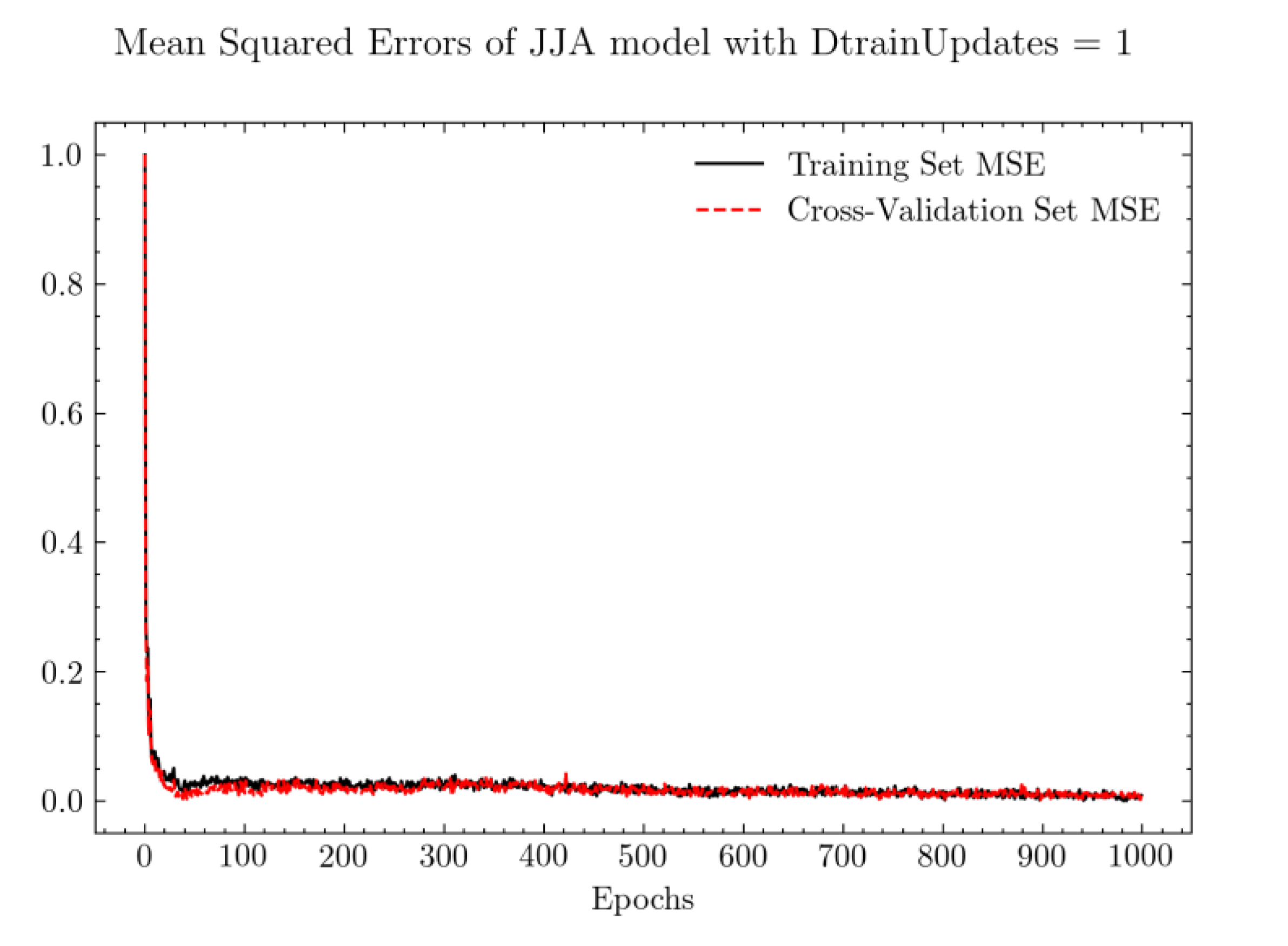
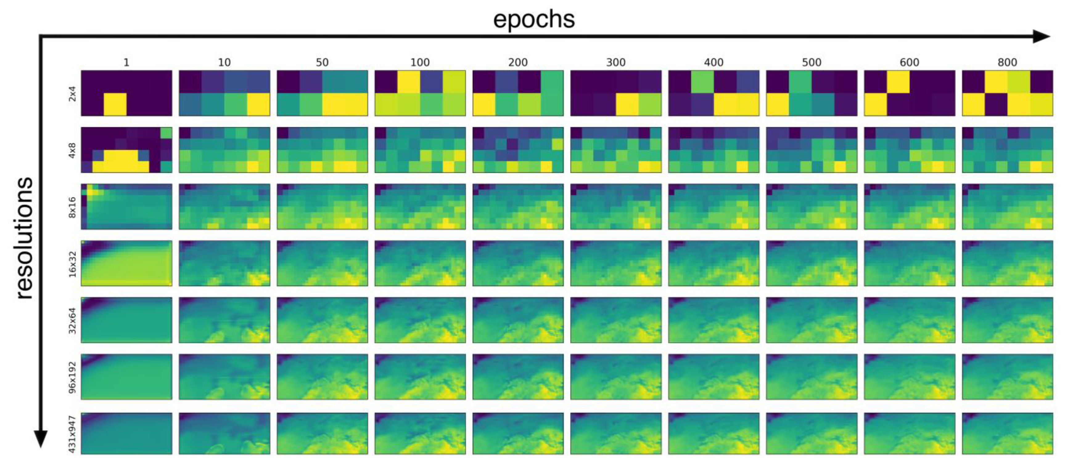
3.1. Training Results

Figure 2 reports the MSE calculated on random training batches of the aforementioned model. Both errors exhibit an early decreasing behavior that leads to a substantial stable convergence in the last epochs. This indicates that the mapping was learnt very quickly, starting around the 50th epoch. The remaining training time was used to improve the model perception capabilities, learning complex details, geometric structures, and high-frequency details, and to enhance sample diversity. Despite this, in the last epochs, the errors did not change significantly. The simultaneous training of all MSG-GAN-SD multi-scale layers makes each epoch slower (especially for models with DtrainUpdates equal to 2 or 3), but fewer epochs were needed for reaching convergence. This means that the overall time required to train the model was reduced compared to that of traditional GANs [15].
Figure 3 reports the resulting generated images of a single fixed sample along the training epochs and resolutions. Throughout the training, all the scales synchronize with each other and mature together during the epochs in terms of accuracy and perceptivity. Concerning the training time performance, the average execution time of each experiment is reported in Table 1. It must be remarked that the experiments were run under the operative conditions explained in Section 2.

3.2. Evaluation Procedure
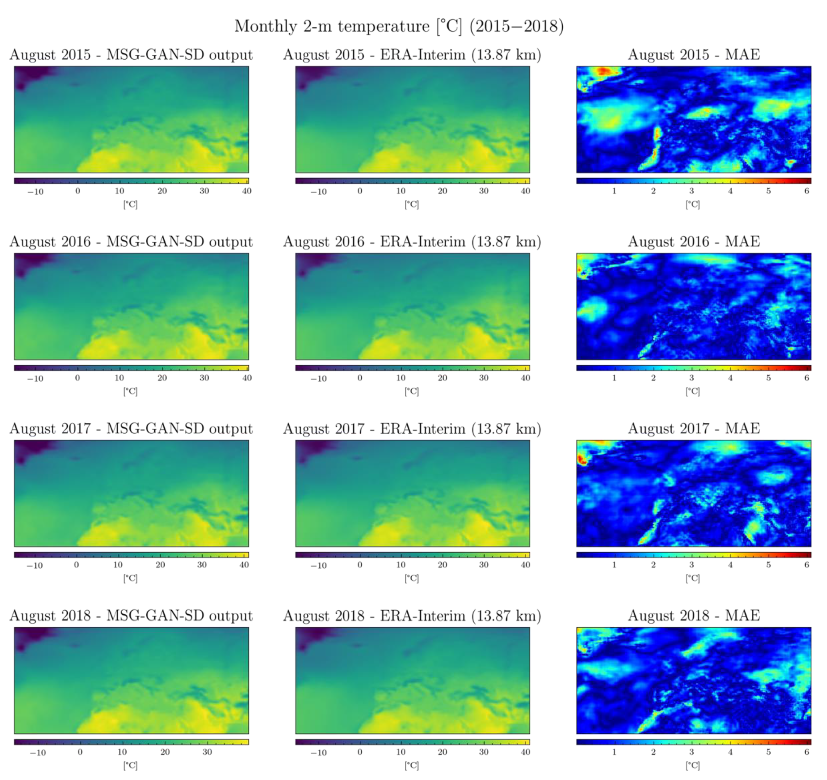
Table A3 reported in Appendix B shows the number of discriminator updates in the training phase (DtrainUpdates) and the selected epoch of the best models, for both month- and season-based arrangements. For each of the three DtrainUpdates models, the best epoch was obtained by applying Equation (1), then the best model was the one that produced the highest 5 f A P P score after a test cycle. As shown in Table A3, there was no evidence of the improvement caused by training D more times than G in a single epoch.
Table A4 and Table A5 in Appendix B report the outputs of the evaluation procedure on the test set, for both monthly and seasonal models’ outcomes, respectively. For each considered month, it is evident from the 5 f A P P metric (higher is better) that the seasonal models perform better against the respective monthly models during the test set years (2015–2018). Evidently, still looking at the 5 f A P P metric, they reach a sort of best trade-off among all the metrics involved in the Accuracy and Perceptivity terms. Thus, the higher number of samples in seasonal dataset arrangements was of greater benefit than the more specific climate dynamics exhibited by the monthly arrangements. Moreover, from a practical standpoint, it is more convenient to manage four seasonal models rather than twelve monthly ones. According to the 5 f A P P , it is be easily noted that the JJA model was found to be the best among the seasonal models, because the metric scores on the average are higher than those reported for the months in the other seasons (see Table A5 in Appendix B). Additionally, the JJA model reached the highest 5 f A P P score in predicting the August month.

3.3. Test Results

Figure 4 shows the results generated by the JJA model in August (left panel), in addition to the ground truth (center panel) and the MAE (right panel). In all cases, the generated and real maps appear to be nearly indistinguishable. In fact, the MAE maps in Figure 4 are mainly blue or dark blue, representing a low error. However, there are recurrent regions in which the behavior is not as good with errors greater than 1 degree, as shown by critical yellow and light blue zones. Additionally, the highest errors (red hotspots) are mainly located in the North-West zone, where very low T2M values are recorded in the ground truth images. Consequently, the weight of the unavoidable error in the network forecasting phase is greater at very low real values. These errors may also depend on the use of a large amount of data during the network training phase. High temporal resolution data (6-hourly) has actually been used, which allowed for training the deep architecture introduced in the present work. By doing this, overfitting could be avoided but, at the same time, it inevitably led to fitting the noise due to day and night cycles that characterize the daily temperature trend. An alternative solution may be considering data at a coarser time resolution (e.g., daily or monthly) with an inevitable reduction in the number of samples available for the training phase. It would therefore be necessary to extend the time interval of the analysis (longer than 40 years) or look for simpler architectural solutions requiring fewer data. In addition, as a pre-processing step, each data sample may be expressed as an anomaly with respect to the daily or monthly average, in order to potentially fasten convergence. Nonetheless, the critical hotspots are mitigated by the interannual mean shown in Figure 5, at the expense of an increased error in the remaining zones. Figure 6 and Figure 7 present, respectively, the monthly and interannual monthly means of Pearson (left panel) and Spearman (center panel) correlation metrics, along with the Spearman associated p-value with a confidence interval (CI) of 95% (right panel). The latter values were computed between the ground truth samples and those generated by the JJA model in August. Looking at these maps, it can be observed that there exists a positive moderate-to-strong correlation—of both Pearson and Spearman types—between generated and real samples, mostly in land areas. This correlation is higher than in sea areas, where there still exists a negative moderate-to-weak correlation. However, there are also some infrequent sea area hotspots in which a modest correlation exists. Considering the Spearman associated p-value, there exist some border-like zones, mostly located in the Western and Northern regions, where the non-linear correlation is not statistically significant (p-value > 0.05).
The complete collection of the rest of the monthly and interannual monthly means comparisons is available at: https://drive.google.com/drive/folders/1GenkyhZHDGxfTF2K12lw2-5dxbkjFLpW?usp=sharing, (accessed on 14 November 2021). The considered architecture required about 43.942 s (on average) to predict a particular month for all test set years. Each atomic sample was processed in about 0.090 s on average. The aforementioned times were computed by averaging the execution times of all test runs. All these tests have been carried out by exploiting only one GPU on a single node of the cluster mentioned in Section 2.

4. Conclusions

This work is the first attempt to use the MSG-GAN architecture for statistical downscaling. The proposed architecture was used for downscaling 2 m temperature from the resolution of 83.25 to 13.87 km over the EURO-CORDEX domain. The season-based training set arrangement was found to overcome the monthly one. Formally, this was confirmed by means of a novel metric—the 5 f A P P —introduced in the present study to simultaneously take both Accuracy and Perceptivity issues into account. In fact, the quality of the images generated by MSG-GAN-SD is very high as they appear nearly indistinguishable from the ground truth samples. However, some critical hotspots were highlighted in the North-West area of the EURO-CORDEX domain, and these are worth of further investigations in order to improve the overall MSG-GAN-SD accuracy. From a computational standpoint, the training of a seasonal model on 36 years of the corresponding season required three days in the worst case (DtrainUpdates = 3), exploiting all the four GPUs of a single node. Clearly, the use of more compute nodes would have led to a significant reduction in the training time. Moreover, the inference phase for each month required less than a minute, considering the four years of the test set. The present work is not aimed at providing a comparison between MSG-GAN-SD output and other downscaling approaches, and the authors leave this kind of investigation for future work. Obviously, errors should be further reduced for this approach to be operationally adopted in climate science. Additional architectural variants shall therefore be taken into consideration as future work. Moreover, a new dataset with either a daily or a monthly temporal resolution will also be considered to avoid the noise coming from daily temperature cycles. Over all, the solution presented in this work paves the way for possible scenarios regarding the climate science context and the use of DL techniques coming from the SISR image processing domain, which offer flexible, powerful and computationally convenient solutions. The authors also intend to experiment with the introduction of additional climatic fields providing more information as inputs, in addition to the explicit embedding of the temporal dimension.

Author Contributions

Conceptualization, G.A. (Giovanni Aloisio), G.A. (Gabriele Accarino), M.C. and F.I.; methodology, G.A. (Gabriele Accarino) and M.C.; software, G.A. (Gabriele Accarino), M.C., F.I., V.A. and A.G.; validation, G.A. (Gabriele Accarino), M.C., F.I., V.A. and A.G.; formal analysis, G.A. (Giovanni Aloisio), G.A. (Gabriele Accarino), M.C.; investigation, G.A. (Giovanni Aloisio), G.A. (Gabriele Accarino), M.C.; resources, G.A. (Gabriele Accarino), M.C., F.I., V.A. and A.G.; data curation, G.A. (Gabriele Accarino), M.C., F.I., V.A., A.G.; writing—original draft preparation, G.A. (Gabriele Accarino), M.C. and F.I.; writing—review and editing, G.A. (Giovanni Aloisio), G.A. (Gabriele Accarino), M.C., F.I., V.A. and A.G.; visualization, G.A. (Gabriele Accarino), M.C., F.I., V.A. and A.G.; supervision, G.A. (Giovanni Aloisio); project administration, G.A. (Giovanni Aloisio); funding acquisition, Not Applicable. All authors have read and agreed to the published version of the manuscript.

Funding

This research received no external funding.

Institutional Review Board Statement

Not applicable.

Informed Consent Statement

Not applicable.

Data Availability Statement

Publicly available datasets were used in this study. The ERA-Interim dataset can be found at the following link: https://apps.ecmwf.int/datasets/data/interim-full-daily/levtype=sfc/ (accessed on 14 November 2021).

Acknowledgments

The authors would like to thank the HPC group at CINECA for their support and for providing computing resources. Moreover, the authors would like to acknowledge Antonio Navarra (CMCC President), Pasquale Schiano, Paola Mercogliano and Marianna Adinolfi (CMCC REHMI Division) for the background information and the suggestions about the dynamical downscaling operational chain running at the CMCC Supercomputing Center, and Antonio Aloisio (CMCC ASC Division) for his editing and proofreading work on this paper.

Conflicts of Interest

The authors declare no conflict of interest.

Appendix A. The MSG-GAN-SD Architecture

Table A1 and Table A2 report the internal structure of the generator and the discriminator within the MSG-GAN-SD architecture, respectively.
Table A1. Generator architecture for the MSG-GAN-SD.
BlockLayerActivationOutput Shape
0.Input
Conv 1 × 1
Conv 2 × 2

LReLU
LReLU
2 × 4 × 1
2 × 4 × 480
2 × 4 × 480
G 0 Conv 1 × 1Tanh2 × 4 × 1
1.Input
Upsampling (2, 2)
Conv 3 × 3
Conv 3 × 3


LReLU
LReLU
2 × 4 × 480
4 × 8 × 480
4 × 8 × 480
4 × 8 × 480
G 1 Conv 1 × 1Tanh4 × 8 × 1
2.Input
Upsampling (2, 2)
Conv 3 × 3
Conv 3 × 3


LReLU
LReLU
4 × 8 × 480
8 × 16 × 480
8 × 16 × 240
8 × 16 × 240
G 2 Conv 1 × 1Tanh8 × 16 × 1
3.Input
Upsampling (2, 2)
Conv 3 × 3
Conv 3 × 3


LReLU
LReLU
8 × 16 × 240
16 × 32 × 240
16 × 32 × 120
16 × 32 × 120
G 3 Conv 1 × 1Tanh16 × 32 × 1
4.Input
Upsampling (2, 2)
Conv 3 × 3
Conv 3 × 3


LReLU
LReLU
16 × 32 × 120
32 × 64 × 120
32 × 64 × 60
32 × 64 × 60
G 4 Conv 1 × 1Tanh32 × 64 × 1
5.Input
Upsampling (3, 3)
Conv 3 × 3
Conv 3 × 3


LReLU
LReLU
32 × 64 × 60
96 × 192 × 60
96 × 192 × 20
96 × 192 × 20
G 5 Conv 1 × 1Tanh96 × 192 × 1
6.Input
Upsampling (5, 5)
Conv 3 × 3
Conv 3 × 3
Conv 3 × 3


LReLU
LReLU
Tanh
96 × 192 × 20
480 × 960 × 20
480 × 960 × 4
480 × 960 × 4
480 × 960 × 1
Table A2. Discriminator architecture for the MSG-GAN-SD.
BlockLayerActivationOutput Shape
0.Input
Conv 3 × 3
MiniBatchStd
Conv 3 × 3
Conv 3 × 3
AvgPool (5, 5)

LReLU

LReLU
LReLU
480 × 960 × 1
480 × 960 × 4
480 × 960 × 5
480 × 960 × 4
480 × 960 × 20
96 × 192 × 20
A u x 0 Auxiliary Image96 × 192 × 1
1.Input
Concat
MiniBatchStd
Conv 3 × 3
Conv 3 × 3
AvgPool (3, 3)


LReLU
LReLU
96 × 192 × 20
96 × 192 × 21
96 × 192 × 22
96 × 192 × 20
96 × 192 × 60
32 × 64 × 60
A u x 1 Auxiliary Image32 × 64 × 1
2.Input
Concat
MiniBatchStd
Conv 3 × 3
Conv 3 × 3
AvgPool (2, 2)


LReLU
LReLU
32 × 64 × 60
32 × 64 × 61
32 × 64 × 62
32 × 64 × 60
32 × 64 × 120
16 × 32 × 120
A u x 2 Auxiliary Image16 × 32 × 1
3.Input
Concat
MiniBatchStd
Conv 3 × 3
Conv 3 × 3
AvgPool (2, 2)


LReLU
LReLU
16 × 32 × 120
16 × 32 × 121
16 × 32 × 122
16 × 32 × 120
16 × 32 × 240
8 × 16 × 240
A u x 3 Auxiliary Image8 × 16 × 1
4.Input
Concat
MiniBatchStd
Conv 3 × 3
Conv 3 × 3
AvgPool (2, 2)


LReLU
LReLU
8 × 16 × 240
8 × 16 × 241
8 × 16 × 242
8 × 16 × 240
8 × 16 × 480
4 × 8 × 480
A u x 4 Auxiliary Image4 × 8 × 1
5.Input
Concat
MiniBatchStd
Conv 3 × 3
Conv 3 × 3
AvgPool (2, 2)


LReLU
LReLU
4 × 8 × 480
4 × 8 × 481
4 × 8 × 482
4 × 8 × 480
4 × 8 × 480
2 × 4 × 480
A u x 5 Auxiliary Image2 × 4 × 1
6.Input
Concat
MiniBatchStd
Conv 2 × 2
Conv 2 × 4
Fully Connected


LReLU
LReLU
Linear
2 × 4 × 480
2 × 4 × 481
2 × 4 × 482
2 × 4 × 480
1 × 1 × 480
1 × 1 × 1

Appendix B. Best Model Selection and Evaluation Results

The best model selection is carried out in two phases. In the first phase, a pool of model candidates is chosen using Equation (1). Specifically, for each model, the equation allows selecting the optimal epoch at which both the training error ( M S E t r , e ) and the generalization error ( | M S E t r , e M S E c v , e | ) are minimum, thus meaning that the training process should be stopped at the e b e s t epoch. Both λ t r and λ t r c v are real numbers acting as penalty terms whose values can be arbitrarily selected to prioritize the minimization of M S E t r , e or the absolute difference between M S E t r , e and M S E c v , e . For the sake of simplicity, in the proposed experiments λ t r and λ t r c v were set to 1 in order to equally weight all the metrics involved in the computation. In some cases, a high degree of generalization is requested at the expense of the accuracy loss in approximating the real distribution, or vice versa. Once the selection of the best-epoch model was completed, a total of 48 models for the various seasons/DtrainUpdates and months/DtrainUpdates combinations were analyzed. When testing the models on the test set in the second phase, the best model for each season/month is obtained by selecting the discriminator that has the highest value computed using Equation (2) among the three discriminator update configurations (DtrainUpdates). In particular, Equation (2) is constructed by multiplying the Accuracy and the Perceptivity factors given by the Expressions (A1) and (A2), respectively.
A c c u r a c y = ( λ M S E M S E )   ( λ P S N R   P S N R )   ( λ S S I M   S S I M )
The Accuracy term measures the quantitative information of the image, such as the colors range and peaks information, in addition to the information related to the overall geometric structure of the image (such as lines, contours, polygons, etc.). It has to be as high as possible to obtaining a good image quality. The Perceptivity term relates to the qualitative information of the image and is defined as:
P e r c e p t i v i t y = ( 1 λ F I D   F I D )   ( 1 λ L S D   L S D )
where a high perceptivity means that the image has good photorealistic features and that high frequency details have been successfully learnt during the training phase. In fact, LSD and FID should be as low as possible, so that their reciprocal will be high. The λ coefficients are normalizing factors, which act as weights with respect to the various involved terms, enabling the selection of a trade-off between Accuracy and Perceptivity factors, or even between any of their components. Table A3 shows, for each month and season, the number of discriminator updates for each epoch during the training phase (DtrainUpdates) and the epochs resulting from the minimization of Equation (1). For example, referring to August, the best monthly model was obtained by applying a single update/epoch of the discriminator (DtrainUpdates = 1), and then gathered at epoch 850 of the training. As shown in Table A3, most of the best models for both the monthly and seasonal training arrangements were obtained with a single update per epoch (DtrainUpdates = 1). Four best monthly models were obtained with two updates per epoch (DtrainUpdates = 2), whereas four best seasonal models and two best monthly models were achieved with three updates per epoch (DtrainUpdates = 3). It can thus be stated that, for this specific use case, there is no evidence of the improvement caused by training D more times than G in a single epoch with relation to the seasonal models. This may be due to the higher number of samples occurring in seasonal models, which can strongly widen the already existing architectural gap (i.e., number of parameters) between D and G. By comparison, the different DtrainUpdates variants in the monthly models are worth considering in order to improve performance, because it is not possible to highlight a clear majority pattern.
Table A3. Best models’ properties.
Training Set ArrangementsMonthlySeasonal
Months# D updatesEpoch# D updatesEpoch
January29501850
February15001850
March185011000
April260011000
May37503350
June28501800
July18001800
August18501800
September27503750
October19503750
November36003750
December19501850
The following tables report the outputs of the evaluation procedure for the monthly and seasonal models’ outcomes, respectively. In Table A4, for each month, the best trained model was tested on the month itself through the test set years (2015–2018). The upward arrows mean that the metrics value has to be as high as possible, whereas the downward arrows mean the opposite. In Table A5 for each season, the best trained model was tested on each month belonging to the corresponding season, during the test set period (2015–2018). The upward arrows mean that the metrics value has to be as high as possible, whereas the downward arrows mean the opposite. All the errors and metrics shown in these tables are calculated on samples normalized in the [−1; 1] interval. Concerning the 5 f A P P metric, all the normalizing coefficients λ in Equation (2) were set to 1, in order to give equal importance to all the involved terms.
Table A4. Evaluation results based on monthly models’ outcomes.
Monthly-Based TrainingMSE (↓)PSNR (↑)SSIM (↑)FID (↓)LSD (↓)Accuracy (↑)Perceptivity (↑) 5 f A P P   ( )
January0.01217.4780.8110.0998.2941173.5851.2131423.007
February0.01018.0520.8340.0628.0861526.1651.9813023.297
March0.00918.5620.8420.0518.9181746.3892.2083856.081
April0.00918.5070.8390.0479.7611697.0902.1803699.364
May0.01018.1370.7990.0669.5051455.6841.5852307.581
June0.00620.2840.8310.0679.1922844.6031.6314639.858
July0.00620.0090.8120.0649.2452548.7371.6974325.116
August0.00520.6920.8360.0457.9603502.8192.8229885.056
September0.00719.8400.8940.0637.7672580.7082.0535298.983
October0.00720.0400.9050.0468.3782602.5562.5736697.147
November0.00919.3670.8770.0917.8931940.0071.3962708.218
December0.01018.6990.8530.0828.4161545.1171.4572251.966
Table A5. Evaluation results based on seasonal models’ outcomes.
Season-Based TrainingMSE (↓)PSNR (↑)SSIM (↑)FID (↓)LSD (↓)Accuracy (↑)Perceptivity (↑) 5 f A P P (↑)
January0.01117.5840.8170.0798.7601324.2481.4381904.269
February0.00918.4140.8430.0618.3881645.4941.9683239.104
March0.00817.5860.7970.0419.8711651.1742.4784091.508
April0.00718.8370.8730.04210.1202233.0762.3515249.693
May0.00720.0510.9240.0539.6892739.6621.9495340.450
June0.00520.4500.8290.0469.1703110.4532.3827407.763
July0.00521.0840.8730.0378.6993733.9633.10911,607.422
August0.00421.3950.8770.0397.3164217.3813.54014,929.312
September0.00521.6180.9580.0487.0473970.4632.96611,777.042
October0.00520.7310.9080.0437.5383748.5293.08511,565.111
November0.00718.3260.8250.0667.7402138.1941.9544178.579
December0.00918.6770.8520.0728.9731794.0511.5422767.413

References

  1. Vandal, T.; Kodra, E.; Ganguly, S.; Michaelis, A.; Nemani, R.; Ganguly, A. DeepSD: Generating High Resolution Climate Change Projections through Single Image Super-Resolution. In Proceedings of the 23rd ACM SIGKDD International Conference on Knowledge Discovery and Data Mining, Halifax, NS, Canada, 13–17 August 2017. [Google Scholar] [CrossRef]
  2. Vandal, T.; Kodra, E.; Ganguly, S.; Michaelis, A.; Nemani, R.; Ganguly, A. Generating High Resolution Climate Change Projections through Single Image Super-Resolution: An Abridged Version. In Proceedings of the Twenty-Seventh International Joint Conference on Artificial Intelligence, Stockholm, Sweden, 13–19 July 2018. [Google Scholar] [CrossRef] [Green Version]
  3. Baño-Medina, J.; Gutiérrez, J.; Herrera, S. Deep Neural Networks for Statistical Downscaling of Climate Change Projections. In Proceedings of the XVIII Conferencia de la Asociación Española para la Inteligencia Artificial (CAEPIA 2018), Granada, España, 23–26 October 2018; pp. 1419–1424. [Google Scholar]
  4. Baño-Medina, J.; Manzanas, R.; Gutiérrez, J. Configuration and intercomparison of deep learning neural models for statistical downscaling. Geosci. Model Dev. 2020, 13, 2109–2124. [Google Scholar] [CrossRef]
  5. Rodrigues, E.; Oliveira, I.; Cunha, R.; Netto, M. DeepDownscale: A Deep Learning Strategy for High-Resolution Weather Forecast. In Proceedings of the 2018 IEEE 14th International Conference on e-Science (e-Science), Amsterdam, The Netherlands, 29 October–1 November 2018. [Google Scholar] [CrossRef] [Green Version]
  6. Wood, A.; Leung, L.; Sridhar, V.; Lettenmaier, D.P. Hydrologic implications of dynamical and statistical approaches to downscaling climate model outputs. Clim. Chang. 2004, 62, 189–216. [Google Scholar] [CrossRef]
  7. Fowler, H.J.; Blenkinsop, S.; Tebaldi, C. Linking climate change modelling to impacts studies: Recent advances in downscaling techniques for hydrological modelling. Int. J. Climatol. 2007, 27, 1547–1578. [Google Scholar] [CrossRef]
  8. Maraun, D.; Widmann, M. Statistical Downscaling and Bias Correction for Climate Research; Cambridge University Press: Cambridge, UK, 2018. [Google Scholar]
  9. Yang, W.; Zhang, X.; Tian, Y.; Wang, W.; Xue, J.; Liao, Q. Deep Learning for Single Image Super-Resolution: A Brief Review. IEEE Trans. Multimed. 2019, 21, 3106–3121. [Google Scholar] [CrossRef] [Green Version]
  10. Leinonen, J.; Nerini, D.; Berne, A. Stochastic Super-Resolution for Downscaling Time-Evolving Atmospheric Fields with a Generative Adversarial Network. IEEE Trans. Geosci. Remote Sens. 2021, 59, 7211–7223. [Google Scholar] [CrossRef]
  11. Wang, Z.; Chen, J.; Hoi, S. Deep Learning for Image Super-resolution: A Survey. IEEE Trans. Pattern Anal. Mach. Intell. 2021, 43, 3365–3387. [Google Scholar] [CrossRef] [PubMed] [Green Version]
  12. Vandal, T.; Kodra, E.; Ganguly, A. Intercomparison of machine learning methods for statistical downscaling: The case of daily and extreme precipitation. Theor. Appl. Climatol. 2019, 137, 557–570. [Google Scholar] [CrossRef] [Green Version]
  13. Pan, B.; Hsu, K.; AghaKouchak, A.; Sorooshian, S. Improving precipitation estimation using convolutional neural network. Water Resour. Res. 2019, 55, 2301–2321. [Google Scholar] [CrossRef] [Green Version]
  14. Sachindra, D.; Ahmed, K.; Rashid, M.; Shahid, S.; Perera, B. Statistical downscaling of precipitation using machine learning techniques. Atmos. Res. 2018, 212, 240–258. [Google Scholar] [CrossRef]
  15. Karnewar, A.; Wang, O. MSG-GAN: Multi-Scale Gradients for Generative Adversarial Networks. In Proceedings of the 2020 IEEE/CVF Conference on Computer Vision and Pattern Recognition (CVPR), Seattle, WA, USA, 13–19 June 2020; pp. 7796–7805. [Google Scholar] [CrossRef]
  16. ERA-Interim. ECMWF. 2020. Available online: https://apps.ecmwf.int/datasets/data/interim-full-daily/levtype=sfc/ (accessed on 14 November 2021).
  17. Wilby, R.; Charles, S.; Zorita, E.; Timbal, B.; Whetton, P.; Mearns, L. Guidelines for Use of Climate Scenarios Developed from Statistical Downscaling Methods. Supporting Material to the IPCC; 2004; pp. 3–21. Available online: https://www.narccap.ucar.edu/ (accessed on 14 November 2021).
  18. Gao, L.; Schulz, K.; Bernhardt, M. Statistical Downscaling of ERA-Interim Forecast Precipitation Data in Complex Terrain Using LASSO Algorithm. Adv. Meteorol. 2014, 2014, 472741. [Google Scholar] [CrossRef] [Green Version]
  19. Coulibaly, P. Downscaling daily extreme temperatures with genetic programming. Geophys. Res. Lett. 2004, 31. [Google Scholar] [CrossRef]
  20. Sachindra, D.; Kanae, S. Machine learning for downscaling: The use of parallel multiple populations in genetic programming. Stoch. Environ. Res. Risk Assess. 2019, 33, 1497–1533. [Google Scholar] [CrossRef] [Green Version]
  21. Bartkowiak, P.; Castelli, M.; Notarnicola, C. Downscaling Land Surface Temperature from MODIS Dataset with Random Forest Approach over Alpine Vegetated Areas. Remote Sens. 2019, 11, 1319. [Google Scholar] [CrossRef] [Green Version]
  22. Anh, Q.T.; Taniguchi, K. Coupling dynamical and statistical downscaling for high-resolution rainfall forecasting: Case study of the Red River Delta, Vietnam. Prog. Earth Planet. Sci. 2018, 5. [Google Scholar] [CrossRef]
  23. Salimi, A.; Samakosh, J.M.; Sharifi, E.; Hassanvand, M.; Noori, A.; von Rautenkranz, H. Optimized Artificial Neural Networks-Based Methods for Statistical Downscaling of Gridded Precipitation Data. Water 2019, 11, 1653. [Google Scholar] [CrossRef] [Green Version]
  24. Min, X.; Ma, Z.; Xu, J.; He, K.; Wang, Z.; Huang, Q.; Li, J. Spatially Downscaling IMERG at Daily Scale Using Machine Learning Approaches Over Zhejiang, Soualthoughtheastern China. Front. Earth Sci. 2020, 8. [Google Scholar] [CrossRef]
  25. Hochreiter, S.; Schmidhuber, J. Long Short-Term Memory. Neural Comput. 1997, 9, 1735–1780. [Google Scholar] [CrossRef]
  26. Misra, S.; Sarkar, S.; Mitra, P. Statistical downscaling of precipitation using long short-term memory recurrent neural networks. Theor. Appl. Climatol. 2017, 134, 1179–1196. [Google Scholar] [CrossRef]
  27. Anh, D.T.; Van, S.; Dang, T.; Hoang, L. Downscaling rainfall using deep learning long short-term memory and feedforward neural network. Int. J. Climatol. 2019, 39, 4170–4188. [Google Scholar] [CrossRef]
  28. Dong, C.; Loy, C.; He, K.; Tang, X. Learning a Deep Convolutional Network for Image Super-Resolution. Lect. Notes Comput. Sci. 2014, 8692, 184–199. [Google Scholar] [CrossRef]
  29. Dong, C.; Loy, C.; He, K.; Tang, X. Image Super-Resolution Using Deep Convolutional Networks. IEEE Trans. Pattern Anal. Mach. Intell. 2016, 38, 295–307. [Google Scholar] [CrossRef] [Green Version]
  30. Kim, J.; Lee, J.K.; Lee, K.M. Accurate image super-resolution using very deep convolutional networks. In Proceedings of the IEEE Conference on Computer Vision and Pattern Recognition (CVPR), Las Vegas, NV, USA, 27–30 June 2016. [Google Scholar] [CrossRef] [Green Version]
  31. Johnson, J.; Alahi, A.; Fei-Fei, L. Perceptual losses for real-time style transfer and super-resolution. In Computer Vision—ECCV 2016, Proceedings of the 14th European Conference, Proceedings, Part II, Amsterdam, The Netherlands, 11–14 October 2016; Leibe, B., Matas, J., Sebe, N., Welling, M., Eds.; Springer: Cham, Switzerland, 2016; pp. 694–711. [Google Scholar] [CrossRef]
  32. Kim, H.; Choi, M.; Lim, B.; Lee, K. Task-Aware Image Downscaling. In Proceedings of the European Conference on Computer Vision (ECCV), Munich, Germany, 8–14 September 2018. [Google Scholar]
  33. Park, D.; Kim, J.; Chun, S.Y. Down-Scaling with Learned Kernels in Multi-Scale Deep Neural Networks for Non-Uniform Single Image Deblurring. arXiv 2019, arXiv:1903.10157. [Google Scholar]
  34. Miao, Q.; Pan, B.; Wang, H.; Hsu, K.; Sorooshian, S. Improving Monsoon Precipitation Prediction Using Combined Convolutional and Long Short Term Memory Neural Network. Water 2019, 11, 977. [Google Scholar] [CrossRef] [Green Version]
  35. Sun, L.; Lan, Y. Statistical downscaling of daily temperature and precipitation over China using deep learning neural models: Localization and comparison with other methods. Int. J. Climatol. 2020. [Google Scholar] [CrossRef]
  36. Huang, X. Deep-Learning Based Climate Downscaling Using the Super-Resolution Method: A Case Study over the Western US. Geosci. Model Dev. Discuss. 2020, preprint. [Google Scholar] [CrossRef]
  37. Kern, M.; Höhlein, K.; Hewson, T.; Westermann, R. Towards Operational Downscaling of Low Resolution Wind Fields Using Neural Networks. In Proceedings of the 22nd EGU General Assembly, EGU2020-5447. Online, 4–8 May 2020. [Google Scholar] [CrossRef]
  38. Shi, X. Enabling Smart Dynamical Downscaling of Extreme Precipitation Events with Machine Learning. Geophys. Res. Lett. 2020, 47. [Google Scholar] [CrossRef]
  39. Sekiyama, T. Statistical Downscaling of Temperature Distributions from the Synoptic Scale to the Mesoscale Using Deep Convolutional Neural Networks. arXiv 2020, arXiv:2007.1083. [Google Scholar]
  40. Wang, X.; Yu, K.; Wu, S.; Gu, J.; Liu, Y.; Dong, C.; Qiao, Y.; Loy, C.C. ESRGAN: Enhanced Super-Resolution Generative Adversarial Networks. Lect. Notes Comput. Sci. 2019, 11133. [Google Scholar] [CrossRef] [Green Version]
  41. Singh, A.; Albert, A.; White, B. Downscaling numerical weather models with gans. In Proceedings of the 9th International Conference on Climate Informatics 2019, Paris, France, 2–4 October 2019; pp. 275–278. [Google Scholar]
  42. Groenke, B.; Madaus, L.; Monteleoni, C. ClimAlign: Unsupervised statistical downscaling of climate variables via normalizing flows. In Proceedings of the 10th International Conference on Climate Informatics, Oxford, UK, 22–25 September 2020. [Google Scholar]
  43. Mendes, D.; Marengo, J. Temporal downscaling: A comparison between artificial neural network and autocorrelation techniques over the Amazon Basin in present and future climate change scenarios. Theor. Appl. Climatol. 2009, 100, 413–421. [Google Scholar] [CrossRef]
  44. Mouatadid, S.; Easterbrook, S.; Erler, A.R. A Machine Learning Approach to Non-uniform Spatial Downscaling of Climate Variables. In Proceedings of the 2017 IEEE International Conference on Data Mining Workshops (ICDMW), New Orleans, LA, USA, 18–21 November 2017; pp. 332–341. [Google Scholar] [CrossRef]
  45. Chang, Y.; Acierto, R.; Itaya, T.; Akiyuki, K.; Tung, C. A Deep Learning Approach to Downscaling Precipitation and Temperature over Myanmar. EGU Gen. Assem. Conf. Abstr. 2018, 4120. [Google Scholar] [CrossRef]
  46. Liu, Y.; Yang, Y.; Jing, W.; Yue, X. Comparison of Different Machine Learning Approaches for Monthly Satellite-Based Soil Moisture Downscaling over Northeast China. Remote Sens. 2018, 10, 31. [Google Scholar] [CrossRef] [Green Version]
  47. Sharifi, E.; Saghafian, B.; Steinacker, R. Downscaling Satellite Precipitation Estimates with Multiple Linear Regression, Artificial Neural Networks, and Spline Interpolation Techniques. J. Geophys. Res. Atmos. 2019, 124, 789–805. [Google Scholar] [CrossRef] [Green Version]
  48. Höhlein, K.; Kern, M.; Hewson, T.; Westermann, R. A comparative study of convolutional neural network models for wind field downscaling. Meteorol. Appl. 2020, 27. [Google Scholar] [CrossRef]
  49. Xu, R.; Chen, N.; Chen, Y.; Chen, Z. Downscaling and Projection of Multi-CMIP5 Precipitation Using Machine Learning Methods in the Upper Han River Basin. Adv. Meteorol. 2020, 2020, 1–17. [Google Scholar] [CrossRef]
  50. Li, X.; Li, Z.; Huang, W.; Zhou, P. Performance of statistical and machine learning ensembles for daily temperature downscaling. Theor. Appl. Climatol. 2020, 140, 571–588. [Google Scholar] [CrossRef]
  51. Sachindra, D.; Huang, F.; Barton, A.; Perera, B. Least square support vector and multi-linear regression for statistically downscaling general circulation model outputs to catchment streamflows. Int. J. Climatol. 2013, 33, 1087–1106. [Google Scholar] [CrossRef] [Green Version]
  52. Goly, A.; Teegavarapu, R.; Mondal, A. Development and Evaluation of Statistical Downscaling Models for Monthly Precipitation. Earth Interact. 2014, 18, 1–28. [Google Scholar] [CrossRef]
  53. Duhan, D.; Pandey, A. Statistical downscaling of temperature using three techniques in the Tons River basin in Central India. Theor. Appl. Climatol. 2014, 121, 605–622. [Google Scholar] [CrossRef]
  54. EURO-CORDEX. Available online: https://euro-cordex.net/index.php.en (accessed on 14 November 2021).
  55. NetCDF. Available online: https://www.unidata.ucar.edu/software/netcdf/ (accessed on 14 November 2021).
  56. ERA-Interim. Available online: https://www.ecmwf.int/en/forecasts/datasets/reanalysis-datasets/era-interim (accessed on 14 November 2021).
  57. Ledig, C.; Theis, L.; Huszár, F.; Caballero, J.; Cunningham, A.; Acosta, A.; Aitken, A.; Tejani, A.; Totz, J.; Wang, Z.; et al. Photo-Realistic Single Image Super-Resolution Using a Generative Adversarial Network. In Proceedings of the 2017 IEEE Conference on Computer Vision and Pattern Recognition (CVPR), Honolulu, HI, USA, 21–26 July 2017; pp. 105–114. [Google Scholar] [CrossRef] [Green Version]
  58. Goodfellow, I.; Pouget-Abadie, J.; Mirza, M.; Xu, B.; Warde-Farley, D.; Ozair, S.; Courville, A.; Bengio, Y. Generative Adversarial Networks. arXiv 2014, arXiv:1406.2661. [Google Scholar] [CrossRef]
  59. Gulrajani, I.; Ahmed, F.; Arjovsky, M.; Dumoulin, V.; Courville, A. Improved Training of Wasserstein GANs. Adv. Neural Inf. Process. Syst. 2017, 30, 5767–5777. [Google Scholar]
  60. Karras, T.; Aila, T.; Laine, S.; Lehtinen, J. Progressive Growing of GANs for Improved Quality, Stability and Variation. In Proceedings of the International Conference on Learning Representations (ICLR), Vancouver, CA, Canada, 30 April–3 May 2018. [Google Scholar]
  61. Denton, E.; Chintala, S.; Szlam, A.; Fergus, R. Deep generative image models using a Laplacian pyramid of adversarial networks. In Proceedings of the 28th International Conference on Neural Information Processing Systems (NIPS’15), Montréal, QC, Canada, 7–12 December 2015; Volume 1, pp. 1486–1494. [Google Scholar]
  62. Dinh, L.; Krueger, D.; Bengio, Y. NICE: Non-linear Independent Components Estimation. In Proceedings of the International Conference on Learning Representations (ICLR), San Diego, CA, USA, 7–9 May 2015. [Google Scholar]
  63. Cineca. Available online: https://www.cineca.it (accessed on 14 November 2021).
  64. Marconi 100. Available online: https://www.hpc.cineca.it/hardware/marconi100 (accessed on 14 November 2021).
  65. Keras. Available online: https://keras.io (accessed on 14 November 2021).
  66. Abadi, M.; Barham, P.; Chen, J.; Chen, Z.; Davis, A.; Dean, J.; Devin, M.; Ghemawat, S.; Irving, G.; Isard, M.; et al. TensorFlow: A System for Large-Scale Machine Learning. In Proceedings of the 12th USENIX Symposium on Operating Systems Design and Implementation (OSDI ’16), Savannah, GA, USA, 2–4 November 2016. [Google Scholar]
  67. Distributed Training with TensorFlow. Available online: https://www.tensorflow.org/guide/distributed_training (accessed on 14 November 2021).
  68. Arjovsky, M.; Chintala, S.; Bottou, L. Wasserstein GAN. arXiv 2017, arXiv:1701.07875. [Google Scholar]
  69. Dauphin, Y.; de Vries, H.; Chung, J.; Bengio, Y. RMSProp and Equilibrated Adaptive Learning Rates for Non-Convex Optimization. arXiv 2015, arXiv:1502.04390v1. [Google Scholar]
  70. Wang, Z.; Bovik, A.C.; Sheikh, H.R.; Simoncelli, E.P. Image quality assessment: From error visibility to structural similarity. IEEE Trans. Image Process. 2004, 13, 600–612. [Google Scholar] [CrossRef] [Green Version]
  71. Heusel, M.; Ramsauer, H.; Unterthiner, T.; Nessler, B.; Hochreiter, S. GANs Trained by a Two Time-Scale Update Rule Converge to a Local Nash Equilibrium. Adv. Neural Inf. Process. Syst. 2017, 30, 6626–6637. [Google Scholar]
Figure 1. The proposed MSG-GAN-SD architecture. The overall network architecture is composed of the Generator (G) and the Discriminator (D). The various multi-scale images entering as input to D are generated or real depending on the sample being analyzed.
Ai 02 00036 g001
Figure 2. Comparison between training and cross-validation MSEs along training epochs. The training is related to the JJA model with DtrainUpdates = 1. At each epoch, MSEs were averaged over random batches of 64 samples and scaled in the range [0,1].
Ai 02 00036 g002
Figure 3. Fixed generated sample along different training epochs and resolutions. The training is related to the JJA model with DtrainUpdates = 1.
Ai 02 00036 g003
Figure 4. Monthly means comparison (for each August of every year from 2015 to 2018) among MSG-GAN-SD generated, ground truth (ERA-Interim 13.87 km) and MAE maps. The model used is the JJA model with DtrainUpdates = 1.
Ai 02 00036 g004
Figure 5. Interannual monthly means comparison (for each August of every year from 2015 to 2018) among MSG-GAN-SD generated, ground truth (ERA-Interim 13.87 km) and MAE samples. The model used is the JJA model with DtrainUpdates = 1.
Ai 02 00036 g005
Figure 6. Monthly means of Pearson and Spearman correlation metrics, and the Spearman associated p-value (for each August of every year from 2015 to 2018) between MSG-GAN-SD generated and ground truth (ERA-Interim 13.87 km) samples. The model used is the JJA model with DtrainUpdates = 1.
Ai 02 00036 g006
Figure 7. Interannual monthly means of Pearson and Spearman correlation metrics, and the Spearman associated p-value (for each August of every year from 2015 to 2018) between MSG-GAN-SD generated and ground truth (ERA-Interim 13.87 km) samples. The model used is the JJA model with DtrainUpdates = 1.
Ai 02 00036 g007
Table 1. Training execution time performance.
Training Set ArrangementsMonth-BasedSeason-Based
DtrainUpdates = 1~1 day~2 days
DtrainUpdates = 2~1 day~3 days
DtrainUpdates = 3~2 days~4 days
Publisher’s Note: MDPI stays neutral with regard to jurisdictional claims in published maps and institutional affiliations.

