On the Effectiveness of Leukocytes Classification Methods in a Real Application Scenario

Abstract

Automating the analysis of digital microscopic images to identify the cell sub-types or the presence of illness has assumed a great importance since it aids the laborious manual process of review and diagnosis. In this paper, we have focused on the analysis of white blood cells. They are the body’s main defence against infections and diseases and, therefore, their reliable classification is very important. Current systems for leukocyte analysis are mainly dedicated to: counting, sub-types classification, disease detection or classification. Although these tasks seem very different, they share many steps in the analysis process, especially those dedicated to the detection of cells in blood smears. A very accurate detection step gives accurate results in the classification of white blood cells. Conversely, when detection is not accurate, it can adversely affect classification performance. However, it is very common in real-world applications that work on inaccurate or non-accurate regions. Many problems can affect detection results. They can be related to the quality of the blood smear images, e.g., colour and lighting conditions, absence of standards, or even density and presence of overlapping cells. To this end, we performed an in-depth investigation of the above scenario, simulating the regions produced by detection-based systems. We exploit various image descriptors combined with different classifiers, including CNNs, in order to evaluate which is the most suitable in such a scenario, when performing two different tasks: Classification of WBC subtypes and Leukaemia detection. Experimental results have shown that Convolutional Neural Networks are very robust in such a scenario, outperforming common machine learning techniques combined with hand-crafted descriptors. However, when exploiting appropriate images for model training, even simpler approaches can lead to accurate results in both tasks.

1. Introduction

Blood contains three types of cells: platelets or thrombocytes, red blood cells (RBCs) or erythrocytes, and white blood cells (WBCs) or leukocytes. Platelets play an important role in haemostasis, leading to the formation of blood clots when there is an injury to blood vessels or other haemorrhages [1]. Red blood cells are important for the transport of oxygen from the heart to all tissues and carry away carbon dioxide [2]. White blood cells have important functions for the immune system, as they are the body’s main defence against infection and disease [3]. Consequently, their reliable classification is important for recognising their different types and potential diseases. All leukocytes contain a nucleus and can be grouped into two main types, according to the appearance of the structure: granulocytes and agranulocytes. These broader categories can be further subdivided into five subtypes: the first includes basophils, eosinophils and neutrophils, while lymphocytes and monocytes belong to the second [4]. Some examples are shown in Figure 1.

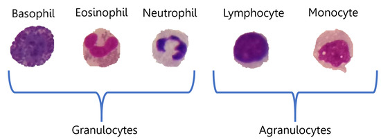
Figure 1. Representation of the WBC sub-types categorisation.

Haematology is the branch of medicine concerned with the study of the blood and the prevention of blood-related diseases. Many diseases can affect the number and type of blood cells produced, their function and lifespan. Usually, only normal, mature or nearly mature cells are released into the bloodstream, but certain circumstances may cause the bone marrow to release immature or abnormal cells into the circulation. Therefore, several manual visual examinations performed by experienced pathologists are essential to detect or monitor these conditions. Microscopic examination of the peripheral blood smear (PBS) slides by clinical pathologists is considered the gold standard for detecting various disorders [5]. Depending on the disorder being inspected (blood cancer, anaemia, presence of parasites), it may require manual counting of cells, classification of cell types and analysis of their morphological characteristics. The disadvantages of this manual inspection are several. It is time-consuming, repetitive and error-prone, and it is subjective because different operators may produce different interpretations of the same scene. Therefore, to avoid misdiagnosis, an automated procedure is increasingly necessary, especially in emerging countries. Among existing blood diseases, leukaemia is a malignant tumour, which can be further grouped into four main types: Acute Lymphoblastic Leukaemia (ALL), Acute Myeloid Leukaemia (AML), Chronic Lymphocytic Leukaemia (CLL), and Chronic Myeloid Leukaemia (CML) [6]. This disease causes the bone marrow to produce abnormal and undeveloped white blood cells, called blasts or leukaemia cells [7]. Their dark purple appearance makes them distinguishable, although analysis and further treatment can be complex due to their variability in shape and consistency. Indeed, different types of WBCs can differ significantly in shape and size, which is one of the most challenging aspects, even considering that they are surrounded by other blood components such as red blood cells and platelets. To address these problems, several computer-aided diagnosis (CAD) systems have been proposed to automate the described manual tasks using image processing techniques and classical Machine Learning (ML) [8,9,10,11,12], and also Deep Learning (DL) approaches [13,14,15], especially after the proposal of Convolutional Neural Network (CNN) [16,17].

CAD systems for PBS analysis can differ greatly from each other because they deal with different medical problems and focus on different tasks, ranging from simple cell counting to complete cell analysis. Despite these significant differences, they generally consist of the same steps: Image pre-processing, segmentation or detection, feature extraction and classification. Not all CAD systems take advantage of all the steps mentioned. As the images captured by new digital microscopes are of excellent quality, the pre-processing step may not be necessary. Furthermore, methods that focus on cell counting do not need feature extraction and classification. On the contrary, some steps may be present several times to address different issues related to the type of images under investigation. For example, multiple segmentation steps might be performed to identify cells and then separate their components. Other times, segmentation steps are combined with detection steps, especially when it is necessary to identify adjacent or clustered cells [10,12,18] As a general rule, CAD systems for PBS analysis can be grouped into two types: segmentation-based or detection-based. Segmentation-based systems are preferred for fine-grained [19] analysis, e.g., for pathology grading, analysis of various cellular components, checking for inclusions or parasites. Detection-based systems, on the other hand, are preferred for quantitative or coarse-grained analyses, such as cataloguing and counting cells [10,12,18,20]. Nowadays, detection-based methods are often preferred to segmentation-based methods, as the generated Bounding Boxes (BBs) can be directly used as input for modern feature extractors or CNNs [21]. Moreover, a particular type of CNNs, Regional CNNs (R-CNNs), perform both the detection phase, mainly exploiting regional proposals, and the classification phase [22]. In this way, it is possible to filter out all those BBs produced by the regional proposal, whose cataloguing process does not reach a high confidence value. However, this process has two main disadvantages: some relevant BBs can be filtered out due to their low confidence value or, even worse, some inaccurate BBs can reach high confidence but with wrong classifications. In this work, we study how accurate the BBs produced by a detection system must be in order to generate a robust classification model and at the same time correctly classify new bounding boxes, both accurate and inaccurate. To this end, we performed several experiments simulating a real-world application scenario in which a model is trained using near-perfect manually annotated BBs and deployed on automatically generated BBs. In the literature, many works deal with the classification of white blood cells [17,23,24,25,26], also proposing Unsupervised Domain Adaptation methods to address the Domain Shift present between different datasets [27]. However, to the best of our knowledge, no one has ever thoroughly investigated whether and to what extent specific features, such as bounding box size and quality, can be crucial for extracting representative features and creating robust models for WBCs classification.

Motivated by these observations, in this work, we propose an in-depth investigation of the above scenario by simulating the BBs produced by detection-based systems with different quality levels. We exploited different image descriptors combined with different classifiers, including CNNs, to assess which is the most suitable in such a scenario in performing two different tasks: Classification of WBC subtypes and Leukaemia detection.

The contribution of this paper is not to create a classification system that can reach or outperform state-of-the-art methods. It instead consists of evaluating the state of the art methods in a scenario different from standard laboratory tests to provide some valuable suggestions/guidelines for creating real CAD systems. For this purpose in our experiments, we performed a quantitative evaluation to assess the single descriptor/classifier; therefore, we discarded all combinations of descriptors or ensembles of classifiers. The rest of the manuscript is organised as follows. Section 2 discusses related work, in particular recent methods for the classification of white blood cells from microscopic images. In Section 3 we illustrate the used data sets, the methods and the experimental setup. The results are presented and discussed in Section 4, and finally, in Section 5 we draw the conclusions and directions for future works.

2. Related Work

Current CAD systems that perform WBC analysis address several tasks ranging from simple counting to disease detection and classification. Since in this work, we focus on two main tasks: Classification of subtypes of WBCs and detection of ALL, in this section, we describe related work that has addressed these two tasks.

Classification of White Blood Cells sub-types. The classification of WBCs sub-types is one of the most ordered laboratory tests since it allows monitoring the proportion of WBCs into the bloodstream that could be affected by numerous diseases and conditions. Even if the WBCs are easily identifiable inside the PBS, this task is very challenging due to wide variations in cell shape, dimensions and edges [1], which are even higher with the presence of a disease. For this reason, most recent works addressing this task exploited CNN-based systems, being more suited to cope with such variability. The authors in [23] performed a concatenation of pre-trained AlexNet and GoogleNet’s feature vectors by taking their maximum values. Then, they classify lymphocytes, monocytes, eosinophils, and neutrophils with the Support Vector Machine (SVM) strategy. The results are higher than 97% for both data sets investigated. Semerjian et al. [24] proposed a built-in customisable CNN, trained with several WBC templates, extracted from the used data set with a segmentation step. They reached a correlation of 90% in recognising different WBCs. Yao et al. [25] proposed a two-module weighted optimised deformable CNN for WBC classification, achieving the best F1-scores (F1) of 95.7%, 94.5% and 91.6% in testing for low-resolution and noisy undisclosed data sets, and BCCD [28] data set, respectively. Qin et al. [17] realised Cell3Net, a fine-grained leukocyte classification method for microscopic images, based on deep residual learning theory and medical domain knowledge. Their method uses a convolutional layer to extract the overall shape feature of the cell body at first, and then three residual blocks (each composed of two convolutional layers and a residual layer) to extract fine features from various aspects. Finally, the last fully connected layers produce a compact feature representation for 40 different types of white blood cells. Ridoy et.al [26] realised a novel CNN architecture to distinguish among eosinophils, lymphocytes, monocytes, and neutrophils, obtaining 86%, 99%, 97%, and 85% of F1-score, respectively.

Acute Lymphoblastic Leukaemia Detection. The detection of a disease is partially related to the previous task since most diseases affect a particular cell sub-types. In particular, ALL affect the lymphocytes that are released prematurely into the bloodstream. Lymphocytes affected by ALL, called lymphoblasts, present morphological changes that increment with increasing severity of the disease [6]. Thus the analysis in this task is more fine-grained, and the systems must distinguish little morphological variations and small cavities inside the nucleus and cytoplasm. Recently, even in this task, CNNs have gained more attention and they have been used both as feature extractor [29,30,31] and to directly classify the images [32,33,34,35,36]. In [32], the author proposed a novel CNN architecture to differentiate normal and abnormal leukocytes, reaching 96.43% accuracy on ALL-IDB1 data set (described in Section 3.1). Khandekar et al. [33] proposed an ALL detection system, composed of a modified version of the YOLOv4 detector, by adjusting the number of filters to support custom data sets used. They reached an F1-score of 92% and weighted F1-score (WFS) of 92% on ALL-IDB1, and C-NMC (accessed on 10 June 2021) [37] data sets, respectively. Mondal et al. [34] proposed a weighted automated CNN-based ensemble model, trained with centre-cropped images to detect ALL. It has been based on Xception, VGG-16, DenseNet-121, MobileNet, and InceptionResNet-V2. They reached 81.6% WFS on C-NMC data set. The authors in [29] used transfer learning to extract images features for further classification from three different CNN architectures both separately and jointly. Moreover, the features were selected according to their gain ratios and used as input to the SVM classifier. The authors also proposed a new, hybrid data set from the union of three distinct databases and aimed to diagnose leukaemia without a segmentation process, achieving accuracy, precision and recall above 99%. Huang et al. [35] realised a WBCs classification framework that combined a modulated Gabor wavelet and deep CNN kernels for each convolutional layer. The authors state that, in this way, the features learned by modulated kernels at different frequencies and orientations are more representative and discriminative for the task. In particular, they tested their method on a data set of hyperspectral images of blood cells. The authors in [30] employed a VGG architecture (described in Section 3.3.3) for extracting features from WBC images and then filtered them using a statistically Enhanced Salp Swarm Algorithm. Finally, using SVM classifier, they reach average accuracy of 96.11%, and 87.9%, on ALL-IDB2, and C-NMC, respectively. Togacar et al. [31] used the Maximal Information Coefficient and Ridge feature selection methods on the combination of features extracted by AlexNet, GoogLeNet, and ResNet-50 (described in Section 3.3.3). Finally, quadratic discriminant analysis was used as a classifier. The overall accuracy on BCCD data set [28] was 97.95% in the classification of white blood cells. In [36], the authors realised a system to classify WBCs through the Attention-aware Residual Network-based Manifold Learning model that exploits the first and second-order category-relevant image-level features. It reached average classification accuracy of 95.3% on a proprietary microscopic WBCs images data set collected from Shandong Shengli Hospital. The authors in [38] proposed a new CNN to deal with ALL detection. They reached an accuracy of 88.25% on a 10-fold cross-validation average. However, they pinpointed that the best fold achieved an accuracy of 99.3%, outperforming most of the works for this task. It appears they cannot outperform the work in [39], which achieved 99.50% accuracy for leukaemia detection on ALL-IDB2 by employing fine-tuned Alexnet and extensive data augmentation, which also comprised an analysis of different colour spaces. Nevertheless, the latter did not specify how they select training and testing samples or use a cross-validation strategy.

In most of the cited works dealing with one of the WBC analysis tasks, the authors have used reference datasets in which the images present single centred cells. It represents the ideal scenario where salient and high discriminative features can be extracted from the images [34]. Of course, this is valid under the assumption that the crops are still performed manually by the pathologists or that the detection systems provide perfect crops. However, this assumption is not verified in real application scenarios, as the systems are fully automated, and therefore the crops are not always precise or perfectly centred. Indeed, the BBs produced by a detection system could be larger, including a large background region, or too narrow and cut off a portion of the cell. Although, until now, no one has performed an exhaustive analysis on this, we believe that these factors can significantly influence the performance of a classification system. For this reason, we performed an in-depth investigation to verify if and to what extent the mentioned issues can affect the performance of automated systems for WBCs sub-type classification and leukaemia detection. Furthermore, we also investigated hand-crafted features combined with common ML methods; even if the reported related work (that are also the most recent) exploited mainly CNN-based methods, they do not provide clear evidence on which one to prefer for this task.

3. Materials and Methods

This section describes the materials and methods used in this work to perform the above evaluation. We first describe the datasets used, the methods employed, and the experimental setup.

3.1. Data Sets

We used two well-known benchmark data sets: the Acute Lymphoblastic Leukaemia Image Database (ALL-IDB) [3], proposed for ALL detection, and Raabin-WBC (R-WBC) [40], a recently proposed data set for WBC sub-types classification.

3.1.1. ALL-IDB2

The ALL-IDB is a dataset of public PBS images from healthy individuals and leukaemia patients, collected at the M. Tettamanti Research Centre for Childhood Leukaemia and Haematological Diseases, Monza, Italy. It is organised in two versions: ALL-IDB1, which presents 108 complete RGB images containing many cells and clusters, and ALL-IDB2, a collection of single WBCs extracted from ALL-IDB1. Since we are only interested in evaluating classification performance in this work, we only used the ALL-IDB2 version. It contains 260 images in JPG format with 24-bit colour depth, and each image presents a single centred leukocyte, 50% of which are lymphoblasts. The images were taken with a light laboratory microscope with different magnifications, ranging from 300 to 500, coupled to two different cameras: an Olympus Optical C2500L and a Canon PowerShot G5. This leads to several variations in terms of colour, brightness, scale and cell size, making this a very challenging dataset. Figure 2 shows a healthy leukocyte and a lymphoblast, taken from ALL-IDB2.

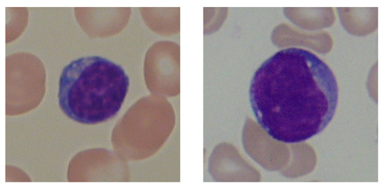
Figure 2. WBC categories from ALL-IDB2: healthy lymphocyte (left) and lymphoblast (right).

3.1.2. R-WBC

R-WBC is a large open-access dataset collected from several laboratories: the Razi Hospital laboratory in Rasht, the Gholhak laboratory, the Shahr-e-Qods laboratory and the Takht-e Tavous laboratory in Tehran, Iran. The images were taken with Olympus CX18 and Zeiss microscopes at 100× magnification, paired with Samsung Galaxy S5 and LG G3 camera smartphones, respectively. For this reason, this data set is also very challenging; even though the scale is fixed, it has several variations in terms of illuminations and colours. After the imaging process, the images were labelled and processed to provide multiple subsets for different tasks. We exploited the subset containing WBC bounding boxes and the ground truth of the nucleus and cytoplasm in this work. This subset contains 1145 images of selected WBCs, including 242 lymphocytes, 242 monocytes, 242 neutrophils, 201 eosinophils and 218 basophils. Thus, unlike the previous data set, the task is to identify the different sub-types of WBCs. A sample image for each WBC sub-type, taken from R-WBC, is shown in Figure 3.

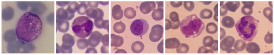
Figure 3. WBC sub-type images from R-WBC. From left to right: Basophil, Eosinophil, Lymphocyte, Monocyte and Neutrophil.

3.2. Data Pre-Processing

As it can be observed from Figure 2 and Figure 3, in both data set images, each WBC is perfectly located in the BB centre and, at the same time, the BB is larger than the WBC size, and many other cells (mainly RBCs) are present in the images. Given that we are investigating how the quality of the extracted BB influences the classification performance, for each original data set, from now on called large, we created three alternative versions from now on called tight, eroded and dilated. As it can be guessed, the tight versions contain images where the BBs are perfectly fit to the WBC size, which should simulate the ideal case. Instead, the remaining versions are the more realistic ones concerning the current detection-based systems, given that in most cases, the provided BBs are not precise. Indeed, it could happen that the WBC is not entirely enclosed inside the BB (like in the eroded version) or that the WBC is not perfectly centred, and a consistent portion of the background is still present in the BB (like in the dilated version). To create these alternative versions, we exploited the pixel-wise ground truth in the form of a binary mask (for ALL-IDB2, whose ground truth was not proposed by the authors, we provided a copy at ALL-IDB2 masks), (accessed on 10 June 2021) where the foreground contains the WBCs only. We extracted the contours extreme points (left, right, top and bottom) to re-crop the RGB images from the foreground. The tight version has been re-cropped, adding just 3 pixels for each side of the box. The eroded/dilated version has been re-cropped, removing/adding 30 pixels for ALL-IDB and 60 pixels for R-WBC (whose resolution is double) from one side of the box randomly drawn. A sample image for each version of healthy leukocyte and lymphoblast, taken from ALL-IDB2 and for each WBC subtype, taken from R-WBC, is shown in Figure 4.

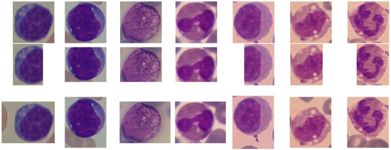
Figure 4. Tight (top), eroded (middle) and dilated (bottom) versions of ALL-IDB2 (first two columns) and R-WBC (remaining columns) data sets.

3.3. Methods

Here we describe the methods used in our evaluation: hand-crafted image descriptors, classic machine learning, and deep learning approaches.

3.3.1. Hand-Crafted Image Descriptors

We evaluated different hand-crafted image descriptors that we grouped into four important classes: invariant moments, texture, colour and wavelet features. As Invariant Moments we computed Legendre and Zernike moments. Legendre moments were first introduced in image analysis by Teague [41] and have been used extensively in many pattern recognition and features extraction applications due to their invariance to scale, rotation and reflection changes [42,43]. They are computed from the Legendre polynomials. Zernike moments also have been used as features set in many applications [44], as they can represent the properties of an image with no redundancy or overlapping of information between moments. They are constructed as the mapping of an image onto a set of complex Zernike polynomials [41]. In both cases, the order of the moments is equal to 5, since a higher-order would have decreased system performance, adding too specif features more useful for image reconstruction rather than for image classification [45].

The Texture Features computed were the rotation invariant Gray Level Co-occurrence Matrix (GLCM) features, as proposed in [46], and the rotation invariant Local Binary Pattern (LBP) features [47]. In both cases we focused on fine textures, thus we computed four GLCMs with $d=1$ and $\theta =[0^{\circ },{45}^{\circ },{90}^{\circ },{135}^{\circ }]$, and the LBP map in the neighbourhood identified by r and n equal to 1 and 8 respectively. From the GLCMs we extracted thirteen features [48] and converted into rotationally invariant ones $Ha{r}_{ri}$ (for more details see [46]). The LBP map is then converted into a rotationally invariant one, and its histogram is used as a feature vector $LB{P}_{ri}$ [47].

As Colour Features, we extracted basic colour histogram and colour auto-correlogram features [49]. The colour histogram features describe the global colour distribution in the image. We computed seven well-known descriptors: mean, standard deviation, smoothness, skewness, kurtosis, uniformity and entropy, which are calculated from images converted in shades of grey. The auto-correlogram combines the colour information with the spatial correlation between colours. In particular, it stores the probability of finding two pixels with the same colour at a distance d. Here, we used four distance values: $d=1,2,3,4$. Finally, the four probability vectors are concatenated to create a single feature vector.

As Wavelet Features, we computed the Gabor [50] and Haar [51] wavelets. Gabor wavelet filter bank is an efficient tool for the analysis of local time-frequency characteristics. It uses a set of specific filters with fixed directions and scales to describe the time-frequency coefficients for each direction and scale. Here we used a common filter bank composed of 40 filters, 5 scales and 8 directions, of size $39\times 39$. Haar wavelet has been used in many different applications, mostly in combination with other techniques. Here we directly applied the Haar wavelet on the original images using three different levels. From each level, we extracted the approximated image and computed the smoothed histogram with 64 bins. The three histograms are finally concatenated to create a single feature vector.

3.3.2. Classic Machine Learning

The classification accuracy was estimated using three different classifiers: the k-Nearest Neighbor (k-NN) classifier [52], the Support Vector Machine (SVM) [53] and Random Forest (RF) [54]. The k-NN was used because it is one of the simplest and can document the effectiveness of the extracted features rather than assessing the classifier’s performance. Here we used $k=1$, computed using the Euclidean distance. The SVM, on the other hand, is one of the most used in biomedical application [12,23,29,30]. Here we use a Gaussian radial basis function (RBF) trained using the one VS rest approach. To speed up the selection of the SVM hyperparameters, we employed an error-correcting output code mechanism [55] with 5-fold cross-validation to fit and automatically tune the hyperparameters. The RF was chosen because it combines many decision trees’ results, thus reducing over-fitting and improving generalisation. Here we used a forest consisting of 100 trees.

3.3.3. Deep Learning

In this work, we also employed DL approaches as both classifier and feature extractor. We evaluated different well known CNN architectures which are: AlexNet, VGG-16, VGG-19, ResNet-18, ResNet-50, ResNet-101, GoogleNet and Inceptionv3. They were all pre-trained on a well-known natural image dataset (ImageNet [56]) and adapted to medical image tasks, following an established procedure for transfer learning and fine-tuning CNN models [57]. AlexNet [16], VGG-16 and the VGG-19 [58] are very simple architectures, but, at the same time, are the most used for transfer learning and fine-tuning [57], since they gained popularity for their excellent performance in many classification tasks [16]. They are quite similar except for the number of layers, which is 8 for AlexNet, 16 for VGG-16 and 19 for VGG-19. The three ResNet architectures are slightly more complex, but being based on residual learning, they are easier to optimise even when the depth increases considerably [59]. They present 18, 50, 101 layers for ResNet-18, ResNet-50 and ResNet-101, respectively. GoogleNet [60] and Inceptionv3 [61] are both based on the Inception layer; indeed, Inceptionv3 is a variant of GoogleNet, exploiting only a few additional layers. They also differ in the number of layers, 100 and 140 for GoogleNet and InceptionV3, respectively. For transfer learning, we followed the approach used in [57], preserving all the CNN layers except the last fully-connected one. We replaced it with a new layer, which has been freshly initialised and set up in order to accommodate the new object categories.

CNNs can be even used to replace traditional feature extractors since they have a solid ability to extract complex features that describe the image in much more detail [31,35]. Therefore we leveraged them both for classification and feature extraction. We acted in different ways depending on the end-use of CNN. We considered the entire CNN architecture by taking its prediction values when used as a classifier, while we only leveraged a portion of CNN when used as a feature extractor. In particular, we extracted features from the penultimate fully connected layer (FC7) on AlexNet, VGG-16 and VGG-19, and the last (only one) on the ResNet and Inception architectures.

3.4. Experimental Setup

In order to perform a fair comparison, we split all the above-mentioned data sets/versions into three parts. Indeed, in order to have a sufficient number of samples for the training process while preserving a sufficient number of samples for performance evaluation, we first split the data sets into two parts, namely training and testing set, with about 70% and 30% of images, respectively. Given that the data sets are well balanced, we used a stratified sampling procedure to keep the splits balanced. Then we further split the original training set into a training and a validation set (used during CNN training), with about 80% and 20% of images, respectively. Even in this split, we have tried to keep intact the proportions between the various classes. Also, to further ease reproducibility, the splits were not created randomly but by taking the images in lexicographic order from each class. We conducted all the experiments on a single machine with the following configuration: Intel(R) Core(TM) i9-8950HK @ 2.90GHz CPU with 32 GB RAM and NVIDIA GTX1050 Ti 4GB GPU.

To evaluate the classification performance, we used five common metrics that are Accuracy (A), Precision (P), Recall (R), Specificity (S) and F1-score (F1). They all range over the interval $[0,1]$. On ALL-IDB, which is a two-class problem, the above metrics are used as they are, while on R-WBC, which is a multi-class problem, the above measures are used to compute the per-class performance, and then, we computed the weighted average to obtain a single performance measure.

As mentioned in Section 3.3.3, we fine-tuned the CNN architectures exploited on both data sets in order to extract more meaningful features. In particular, we used the hyper-parameters defined in Table 1. Furthermore, considering that we did not produce any image augmentation, we set the regularisation factor L₂ in order to avoid a possible over-fitting during the training phase.

Table 1. Hyper-parameters settings for CNNs fine-tuning.

Params	Value
Solver	Adam
Max Epochs	50
Mini Batch Size	8
Initial Learn Rate	1e-4
Learn Rate Drop Period	10
Learn Rate Drop Factor	0.1
L2 Regularisation	0.1

4. Experimental Results

As mentioned before, in this work, we are interested in investigating how the quality of the extracted BB influences the classification performance; thus, we performed different experiments involving the mentioned data sets/versions. The first experiments are devoted to comparing the performance of the different features and classifiers in a controlled (ideal) environment, as it happens in most benchmark data sets created specifically for model training, where the BBs are precise. In this experiments, from now on called “single-version”, we compared the original (large) versions of the data sets with the tight versions in order to evaluate if and to what extent the presence of a large portion of background in the BBs can influence the extracted features and consequently also the created classification models.

The subsequent experiments are devoted to evaluating the robustness of the different features and classifiers in an uncontrolled (real) environment, where the features to train the classification models could still be extracted from controlled benchmark data sets. However, the classification models are deployed in a real scenario. To simulate this scenario in this experiments, from now on called “cross-version”, we exploited the classification models already trained during the previous experiments, that is using the training sets from the large and tight versions of the data sets, but this time they are tested using the test sets belonging to the other versions of the data sets.

4.1. Results

For the sake of brevity, we have reported the results of experiments performed on a single table for each version of the source data sets. It means that in the Table 2 and Table 3 and in the Table 4 and Table 5 we reported the performance obtained when the source models are created exploiting the large and tight versions of the data sets respectively, and then tested using all versions of the data sets (large, tight, eroded and dilated) in turn. To emphasise the performance on the same-version, all corresponding columns in the tables have been highlighted in grey. In addition, we have reported the average performance value of each classifier on the different feature sets to facilitate comparisons.

Table 2. ALL-IDB2 performance obtained with source models created exploiting the large data set version and tested using in turn (from the left) the large, tight, eroded and dilated versions. Same-version performance are highlighted in grey.

Classifier	Descriptor	Target Set
		Large					Tight					Eroded					Dilated
		A	P	R	S	F1	A	P	R	S	F1	A	P	R	S	F1	A	P	R	S	F1
kNN	Legendre	56.4	55.6	64.1	48.7	59.5	52.6	100.0	5.1	100.0	9.8	53.8	80.0	10.3	97.4	18.2	53.8	63.6	17.9	89.7	28.0
	Zernike	35.9	33.3	28.2	43.6	30.6	10.3	10.3	10.3	10.3	10.3	19.2	16.7	15.4	23.1	16.0	21.8	25.0	28.2	15.4	26.5
	HARri	61.5	58.8	76.9	46.2	66.7	50.0	50.0	15.4	84.6	23.5	46.2	36.4	10.3	82.1	16.0	52.6	62.5	12.8	92.3	21.3
	LBP18	53.8	52.5	82.1	25.6	64.0	47.4	48.7	94.9	0.0	64.3	50.0	50.0	100.0	0.0	66.7	47.4	48.7	94.9	0.0	64.3
	Histogram	64.1	60.8	79.5	48.7	68.9	46.2	33.3	7.7	84.6	12.5	47.4	37.5	7.7	87.2	12.8	43.6	27.3	7.7	79.5	12.0
	Correlogram	50.0	50.0	10.3	89.7	17.0	53.8	71.4	12.8	94.9	21.7	47.4	40.0	10.3	84.6	16.3	53.8	61.5	20.5	87.2	30.8
	Haar wavelet	75.6	69.2	92.3	59.0	79.1	70.5	73.5	64.1	76.9	68.5	53.8	53.7	56.4	51.3	55.0	79.5	87.1	69.2	89.7	77.1
	Gabor wavelet	43.6	45.1	59.0	28.2	51.1	60.3	63.3	48.7	71.8	55.1	53.8	54.3	48.7	59.0	51.4	52.6	52.2	61.5	43.6	56.5
	AlexNet	70.5	72.2	66.7	74.4	69.3	75.6	67.2	100.0	51.3	80.4	71.8	69.8	76.9	66.7	73.2	66.7	60.7	94.9	38.5	74.0
	VGG-16	69.2	65.3	82.1	56.4	72.7	66.7	63.3	79.5	53.8	70.5	67.9	64.0	82.1	53.8	71.9	64.1	61.2	76.9	51.3	68.2
	VGG-19	69.2	61.9	100.0	38.5	76.5	83.3	77.1	94.9	71.8	85.1	71.8	66.7	87.2	56.4	75.6	76.9	69.8	94.9	59.0	80.4
	ResNet-18	75.6	67.9	97.4	53.8	80.0	66.7	69.7	59.0	74.4	63.9	60.3	60.0	61.5	59.0	60.8	73.1	73.7	71.8	74.4	72.7
	ResNet-50	82.1	82.1	82.1	82.1	82.1	34.6	33.3	30.8	38.5	32.0	30.8	27.3	23.1	38.5	25.0	52.6	52.9	46.2	59.0	49.3
	ResNet-101	76.9	80.0	71.8	82.1	75.7	46.2	38.5	12.8	79.5	19.2	39.7	10.0	2.6	76.9	4.1	50.0	50.0	20.5	79.5	29.1
	GoogleNet	82.1	77.8	89.7	74.4	83.3	51.3	100.0	2.6	100.0	5.0	50.0	0.0	0.0	100.0	0.0	57.7	100.0	15.4	100.0	26.7
	Inceptionv3	76.9	70.6	92.3	61.5	80.0	33.3	31.4	28.2	38.5	29.7	39.7	30.0	15.4	64.1	20.3	26.9	30.4	35.9	17.9	32.9
	AVG	65.2	62.7	73.4	57.1	66.0	53.0	58.2	41.7	64.4	40.7	50.2	43.5	38.0	62.5	36.4	54.6	57.9	48.1	61.1	46.9
SVMRbf	Legendre	60.3	68.2	38.5	82.1	49.2	48.7	40.0	5.1	92.3	9.1	47.4	40.0	10.3	84.6	16.3	51.3	100.0	2.6	100.0	5.0
	Zernike	41.0	42.6	51.3	30.8	46.5	38.5	41.8	59.0	17.9	48.9	60.3	58.3	71.8	48.7	64.4	48.7	49.2	79.5	17.9	60.8
	HARri	59.0	55.7	87.2	30.8	68.0	52.6	52.9	46.2	59.0	49.3	52.6	53.3	41.0	64.1	46.4	56.4	57.1	51.3	61.5	54.1
	LBP18	61.5	58.2	82.1	41.0	68.1	50.0	50.0	100.0	0.0	66.7	50.0	50.0	100.0	0.0	66.7	50.0	50.0	100.0	0.0	66.7
	Histogram	38.5	35.5	28.2	48.7	31.4	47.4	37.5	7.7	87.2	12.8	46.2	20.0	2.6	89.7	4.5	35.9	7.7	2.6	69.2	3.8
	Correlogram	55.1	53.6	76.9	33.3	63.2	51.3	51.4	48.7	53.8	50.0	47.4	47.2	43.6	51.3	45.3	52.6	52.8	48.7	56.4	50.7
	Haar wavelet	82.1	74.5	97.4	66.7	84.4	50.0	50.0	94.9	5.1	65.5	50.0	50.0	97.4	2.6	66.1	69.2	62.7	94.9	43.6	75.5
	Gabor wavelet	50.0	50.0	76.9	23.1	60.6	64.1	69.0	51.3	76.9	58.8	60.3	65.4	43.6	76.9	52.3	55.1	54.8	59.0	51.3	56.8
	AlexNet	44.9	46.6	69.2	20.5	55.7	67.9	93.8	38.5	97.4	54.5	61.5	100.0	23.1	100.0	37.5	69.2	75.9	56.4	82.1	64.7
	VGG-16	71.8	64.9	94.9	48.7	77.1	69.2	64.7	84.6	53.8	73.3	59.0	56.1	82.1	35.9	66.7	67.9	63.5	84.6	51.3	72.5
	VGG-19	62.8	57.4	100.0	25.6	72.9	74.4	66.1	100.0	48.7	79.6	70.5	62.9	100.0	41.0	77.2	70.5	62.9	100.0	41.0	77.2
	ResNet-18	78.2	71.2	94.9	61.5	81.3	70.5	80.8	53.8	87.2	64.6	62.8	67.9	48.7	76.9	56.7	74.4	80.6	64.1	84.6	71.4
	ResNet-50	83.3	81.0	87.2	79.5	84.0	35.9	33.3	28.2	43.6	30.6	28.2	27.0	25.6	30.8	26.3	44.9	44.1	38.5	51.3	41.1
	ResNet-101	82.1	85.7	76.9	87.2	81.1	73.1	95.0	48.7	97.4	64.4	61.5	90.9	25.6	97.4	40.0	79.5	92.6	64.1	94.9	75.8
	GoogleNet	83.3	79.5	89.7	76.9	84.3	51.3	100.0	2.6	100.0	5.0	50.0	0.0	0.0	100.0	0.0	57.7	100.0	15.4	100.0	26.7
	Inceptionv3	84.6	78.7	94.9	74.4	86.0	64.1	59.6	87.2	41.0	70.8	65.4	62.0	79.5	51.3	69.7	47.4	48.4	76.9	17.9	59.4
	AVG	64.9	62.7	77.9	51.9	68.4	56.8	61.6	53.5	60.1	50.2	54.6	53.2	49.7	59.5	46.0	58.2	62.6	58.7	57.7	53.9
RF	Legendre	60.3	60.0	61.5	59.0	60.8	51.3	100.0	2.6	100.0	5.0	52.6	66.7	10.3	94.9	17.8	57.7	87.5	17.9	97.4	29.8
	Zernike	25.6	25.6	25.6	25.6	25.6	35.9	36.6	38.5	33.3	37.5	26.9	17.9	12.8	41.0	14.9	43.6	40.7	28.2	59.0	33.3
	HARri	52.6	51.6	82.1	23.1	63.4	48.7	47.8	28.2	69.2	35.5	43.6	39.1	23.1	64.1	29.0	56.4	61.9	33.3	79.5	43.3
	LBP18	47.4	48.6	92.3	2.6	63.7	50.0	0.0	0.0	100.0	0.0	50.0	0.0	0.0	100.0	0.0	51.3	100.0	2.6	100.0	5.0
	Histogram	65.4	61.5	82.1	48.7	70.3	60.3	72.2	33.3	87.2	45.6	50.0	50.0	28.2	71.8	36.1	52.6	57.1	20.5	84.6	30.2
	Correlogram	64.1	62.2	71.8	56.4	66.7	59.0	61.3	48.7	69.2	54.3	56.4	57.1	51.3	61.5	54.1	55.1	56.3	46.2	64.1	50.7
	Haar wavelet	46.2	44.8	33.3	59.0	38.2	51.3	53.8	17.9	84.6	26.9	51.3	53.8	17.9	84.6	26.9	53.8	60.0	23.1	84.6	33.3
	Gabor wavelet	42.3	45.2	71.8	12.8	55.4	35.9	40.7	61.5	10.3	49.0	46.2	46.5	51.3	41.0	48.8	39.7	43.1	64.1	15.4	51.5
	AlexNet	60.3	62.5	51.3	69.2	56.3	88.5	96.9	79.5	97.4	87.3	69.2	89.5	43.6	94.9	58.6	69.2	69.2	69.2	69.2	69.2
	VGG-16	71.8	66.7	87.2	56.4	75.6	71.8	66.0	89.7	53.8	76.1	64.1	59.0	92.3	35.9	72.0	70.5	64.8	89.7	51.3	75.3
	VGG-19	65.4	59.1	100.0	30.8	74.3	78.2	73.9	87.2	69.2	80.0	69.2	65.3	82.1	56.4	72.7	80.8	74.0	94.9	66.7	83.1
	ResNet-18	76.9	70.6	92.3	61.5	80.0	67.9	79.2	48.7	87.2	60.3	57.7	59.4	48.7	66.7	53.5	76.9	88.9	61.5	92.3	72.7
	ResNet-50	80.8	78.6	84.6	76.9	81.5	34.6	35.0	35.9	33.3	35.4	30.8	27.3	23.1	38.5	25.0	46.2	45.2	35.9	56.4	40.0
	ResNet-101	79.5	81.1	76.9	82.1	78.9	59.0	66.7	35.9	82.1	46.7	52.6	55.6	25.6	79.5	35.1	62.8	70.8	43.6	82.1	54.0
	GoogleNet	83.3	79.5	89.7	76.9	84.3	51.3	100.0	2.6	100.0	5.0	50.0	0.0	0.0	100.0	0.0	56.4	100.0	12.8	100.0	22.7
	InceptionV3	76.9	70.6	92.3	61.5	80.0	33.3	31.4	28.2	38.5	29.7	39.7	30.0	15.4	64.1	20.3	26.9	30.4	35.9	17.9	32.9
	AVG	62.4	60.5	74.7	50.2	65.9	54.8	60.1	39.9	69.7	42.1	50.6	44.8	32.9	68.4	35.3	56.3	65.6	42.5	70.0	45.5
CNN	AlexNet	44.9	20.5	40.0	46.5	27.1	65.4	94.9	59.7	87.5	73.3	57.7	100.0	54.2	100.0	70.3	71.8	89.7	66.0	84.0	76.1
	VGG-16	61.5	23.1	100.0	56.5	37.5	73.1	56.4	84.6	67.3	67.7	67.9	43.6	85.0	62.1	57.6	70.5	51.3	83.3	64.8	63.5
	VGG-19	57.7	15.4	100.0	54.2	26.7	71.8	59.0	79.3	67.3	67.6	66.7	51.3	74.1	62.7	60.6	70.5	48.7	86.4	64.3	62.3
	ResNet-18	75.6	51.3	100.0	67.2	67.8	66.7	33.3	100.0	60.0	50.0	61.5	23.1	100.0	56.5	37.5	70.5	43.6	94.4	63.3	59.6
	ResNet-50	75.6	64.1	83.3	70.8	72.5	35.9	35.9	35.9	35.9	35.9	25.6	20.5	22.9	27.9	21.6	41.0	41.0	41.0	41.0	41.0
	ResNet-101	75.6	56.4	91.7	68.5	69.8	71.8	59.0	79.3	67.3	67.6	61.5	48.7	65.5	59.2	55.9	70.5	48.7	86.4	64.3	62.3
	GoogleNet	71.8	43.6	100.0	63.9	60.7	66.7	100.0	60.0	100.0	75.0	64.1	100.0	58.2	100.0	73.6	88.5	100.0	81.2	100.0	89.7
	InceptionV3	78.2	64.1	89.3	72.0	74.6	34.6	41.0	36.4	32.3	38.5	39.7	64.1	43.1	30.0	51.5	29.5	23.1	26.5	31.8	24.6
	AVG	67.6	42.3	88.0	62.5	54.6	60.7	59.9	66.9	64.7	59.5	55.6	56.4	62.9	62.3	53.6	64.1	55.8	70.7	64.2	59.9

Table 3. R-WBC performance obtained with source models created exploiting the large data set version and tested using in turn (from the left) the large, tight, eroded and dilated versions. Same-version performance are highlighted in grey.

Classifier	Descriptor	Target Set
		Large					Tight					Eroded					Dilated
		A	P	R	S	F1	A	P	R	S	F1	A	P	R	S	F1	A	P	R	S	F1
kNN	Legendre	75.0	39.1	37.8	84.4	37.9	65.7	22.5	13.7	78.9	11.6	66.3	25.3	15.4	79.3	12.5	67.6	20.7	18.9	80.1	16.8
	Zernike	71.3	28.9	28.5	82.3	28.3	65.8	13.1	15.7	78.4	12.6	69.0	17.1	22.7	80.8	16.4	68.3	20.3	20.6	80.3	16.7
	HARri	70.0	25.3	25.3	81.3	25.2	65.9	16.8	15.1	78.8	13.1	65.7	19.0	14.8	78.4	12.3	64.8	10.0	12.5	78.1	10.0
	LBP18	78.3	47.2	46.2	86.6	46.4	68.1	3.6	18.9	81.1	6.0	68.1	3.6	18.9	81.1	6.0	68.1	3.6	18.9	81.1	6.0
	Histogram	70.2	25.6	26.2	81.4	25.7	69.0	23.3	23.5	80.4	21.8	70.1	24.0	26.5	80.9	23.2	67.2	18.9	18.6	79.2	17.9
	Correlogram	71.1	26.9	27.6	82.3	21.6	69.2	21.3	23.0	81.0	18.3	70.6	26.3	26.7	81.8	23.5	70.6	28.5	26.5	82.0	22.5
	Haar wavelet	79.6	49.9	49.7	87.3	49.3	63.8	14.7	9.3	77.4	10.9	64.4	12.8	11.6	77.6	11.0	63.0	13.2	7.0	77.1	8.8
	Gabor wavelet	74.4	36.9	36.0	84.1	35.1	71.5	28.8	28.8	82.0	23.5	69.6	24.1	23.8	81.2	19.2	72.0	31.3	29.7	82.5	25.5
	AlexNet	97.0	92.9	92.4	98.0	92.3	77.0	45.2	43.3	85.1	36.4	76.2	38.6	41.3	84.6	32.4	80.6	55.1	52.3	87.4	45.5
	VGG-16	98.3	96.0	95.9	98.9	95.9	77.9	56.1	46.5	85.9	40.5	73.4	51.4	35.5	82.8	29.1	82.8	61.9	58.4	89.0	54.6
	VGG-19	95.7	89.2	89.2	97.2	89.1	68.5	20.2	20.9	80.8	10.0	68.1	18.2	19.5	80.9	7.8	70.1	29.5	25.6	81.6	16.5
	ResNet-18	96.3	90.6	90.7	97.7	90.6	72.2	33.6	30.2	83.0	20.2	69.7	42.7	23.3	81.9	13.6	74.2	40.4	35.5	84.2	26.5
	ResNet-50	96.8	92.8	92.2	97.9	92.1	81.5	62.6	55.2	88.0	51.8	77.0	61.0	44.2	85.0	41.3	83.9	63.0	61.0	89.6	57.5
	ResNet-101	98.6	96.5	96.5	99.1	96.5	73.5	37.2	35.8	82.8	28.5	69.7	35.4	26.2	80.2	16.2	78.1	54.5	47.1	86.0	39.5
	GoogleNet	97.7	94.4	94.2	98.5	94.1	77.5	46.6	44.5	85.7	34.6	75.9	43.2	40.7	84.7	28.7	82.5	55.7	57.3	89.0	51.3
	Inceptionv3	98.4	96.4	96.2	99.0	96.2	70.1	59.5	27.3	80.5	19.0	69.3	62.8	25.3	79.9	15.8	72.7	59.4	33.7	82.3	28.7
	AVG	85.5	64.3	64.0	91.0	63.5	71.1	31.6	28.2	81.9	22.4	70.2	31.6	26.0	81.3	19.3	72.9	35.4	32.7	83.1	27.8
SVMRbf	Legendre	77.1	43.1	43.0	85.6	43.0	64.6	18.6	10.8	78.5	6.9	64.5	43.5	11.0	78.1	10.2	69.0	34.3	21.8	81.1	13.8
	Zernike	74.9	35.7	37.8	84.3	35.2	63.6	11.1	9.0	77.4	6.8	68.2	29.3	20.1	80.6	13.6	68.0	12.5	19.5	80.5	11.9
	HARri	74.7	37.4	36.6	84.6	35.0	71.6	23.1	29.4	81.8	24.0	73.1	35.1	33.1	82.8	28.9	70.4	22.8	26.5	81.3	23.2
	LBP18	74.8	42.9	38.1	84.1	39.0	67.7	4.5	21.2	78.8	7.4	67.7	4.5	21.2	78.8	7.4	67.7	4.5	21.2	78.8	7.4
	Histogram	79.6	51.2	49.1	87.8	45.3	62.8	6.1	5.2	77.6	5.0	63.8	6.6	8.4	78.0	6.9	63.5	14.8	7.0	77.9	8.5
	Correlogram	78.4	48.4	46.8	86.5	47.3	72.2	44.4	31.7	82.1	30.5	71.8	43.3	30.8	81.7	28.7	73.8	46.5	35.5	83.1	35.4
	Haar wavelet	82.5	57.4	56.7	89.1	56.6	67.7	15.8	20.1	79.2	12.7	68.8	19.0	23.3	79.8	15.1	67.8	21.1	19.8	79.6	15.0
	Gabor wavelet	79.9	47.7	49.7	87.4	48.4	71.8	34.1	29.9	82.1	24.3	71.4	33.5	29.1	81.8	24.4	73.6	38.3	34.3	83.4	30.3
	AlexNet	98.0	95.2	95.1	98.7	95.0	76.3	50.3	41.6	84.4	33.4	75.2	46.3	39.0	83.7	29.8	80.4	57.6	51.7	87.1	44.6
	VGG-16	98.7	96.8	96.8	99.2	96.8	79.2	55.2	49.4	86.9	42.2	75.1	45.5	39.5	84.1	32.2	83.2	59.5	59.3	89.5	53.8
	VGG-19	96.1	90.0	90.1	97.5	90.1	68.0	4.6	19.2	80.7	7.1	68.0	3.7	18.9	80.9	6.2	68.3	26.4	20.3	80.8	9.6
	ResNet-18	96.2	90.3	90.4	97.6	90.3	70.8	39.7	26.7	82.3	16.9	68.8	37.8	20.9	81.3	9.8	72.8	41.2	32.3	83.3	22.7
	ResNet-50	97.9	95.0	94.8	98.6	94.7	79.6	59.8	50.6	86.8	47.7	73.8	58.2	36.3	82.9	32.2	84.3	62.8	61.9	89.8	58.0
	ResNet-101	98.8	97.1	97.1	99.2	97.1	75.7	37.7	41.3	84.2	31.5	73.9	36.4	36.6	83.0	27.1	77.7	57.9	46.2	85.7	37.8
	GoogleNet	97.7	94.5	94.2	98.5	94.1	74.6	36.2	36.3	84.4	25.6	72.8	34.4	32.0	83.3	20.3	78.5	43.5	46.2	86.6	38.1
	Inceptionv3	98.3	96.0	95.9	98.9	95.9	70.9	59.6	29.4	81.1	21.9	69.0	40.1	24.7	79.7	14.9	74.2	58.4	37.5	83.4	32.4
	AVG	87.7	69.9	69.5	92.3	69.0	71.1	31.3	28.2	81.8	21.5	70.4	32.3	26.6	81.3	19.2	73.3	37.6	33.8	83.2	27.7
RF	Legendre	75.2	38.3	38.4	84.5	38.2	69.2	11.7	21.8	81.5	12.0	67.4	13.9	18.0	80.2	12.4	70.2	24.0	24.7	82.1	15.4
	Zernike	73.2	31.3	33.1	83.5	31.5	65.4	7.7	12.8	79.0	6.3	68.7	16.3	20.9	81.2	12.1	68.3	16.9	19.8	80.9	11.2
	HARri	83.5	60.5	59.0	89.8	59.4	72.6	21.3	31.1	83.2	22.1	70.6	20.3	26.2	82.0	17.0	74.2	47.1	35.8	83.9	28.6
	LBP18	79.9	53.5	49.4	87.8	49.9	68.1	9.8	22.1	79.2	11.0	67.8	13.9	21.5	78.9	9.4	68.8	15.3	23.8	79.7	14.3
	Histogram	81.0	53.9	52.9	88.2	52.6	66.4	46.9	15.7	79.4	13.6	66.2	31.8	14.8	79.3	13.2	67.1	29.4	17.4	79.6	17.3
	Correlogram	79.0	48.5	48.0	87.0	47.9	74.4	36.9	36.3	84.0	31.2	73.4	36.1	34.0	83.4	29.2	75.4	37.6	39.2	84.6	35.3
	Haar wavelet	88.3	71.0	70.6	92.7	70.6	63.7	17.6	8.4	77.7	8.4	63.7	17.0	8.1	77.7	7.5	65.7	30.5	13.7	78.9	14.3
	Gabor wavelet	81.3	51.2	53.2	88.3	51.8	72.3	36.3	30.8	82.5	26.4	70.6	30.6	26.7	81.4	22.5	72.9	32.8	32.3	83.0	27.9
	AlexNet	97.7	94.5	94.2	98.4	94.1	77.8	50.8	45.3	85.6	38.5	76.6	49.1	42.2	84.8	33.5	82.0	55.8	55.5	88.3	47.2
	VGG-16	98.6	96.6	96.5	99.1	96.5	71.1	47.6	29.4	81.2	21.8	68.9	39.6	24.1	79.7	13.2	76.4	53.7	42.2	84.6	38.6
	VGG-19	95.8	89.4	89.5	97.3	89.4	68.3	26.7	20.3	80.8	9.3	67.9	3.9	18.9	80.8	6.5	69.7	28.9	24.4	81.5	15.3
	ResNet-18	96.3	90.5	90.7	97.7	90.6	71.7	39.3	29.4	82.6	18.6	69.2	40.4	22.4	81.4	12.0	72.8	38.9	32.6	83.2	22.3
	ResNet-50	97.7	94.3	94.2	98.5	94.1	75.5	53.5	39.8	84.1	36.3	72.3	51.2	32.0	82.0	25.8	81.0	59.2	53.5	87.8	50.8
	ResNet-101	98.7	96.8	96.8	99.2	96.8	70.3	26.8	25.9	81.3	15.7	69.8	27.0	24.4	81.1	12.5	74.7	50.9	37.2	84.1	29.1
	GoogleNet	97.3	93.7	93.3	98.2	93.3	76.9	46.0	43.3	85.3	33.5	75.6	39.5	40.1	84.5	28.4	81.0	56.0	53.5	87.9	48.3
	Inceptionv3	98.3	96.0	95.9	99.0	95.9	69.4	50.7	25.0	80.2	14.3	68.6	28.9	23.3	79.6	11.8	72.0	51.8	31.1	82.1	23.0
	AVG	88.9	72.5	72.2	93.1	72.0	70.8	33.1	27.3	81.7	19.9	69.8	28.7	24.9	81.1	16.7	73.3	39.3	33.5	83.3	27.4
CNN	AlexNet	98.1	95.5	95.3	98.9	95.4	64.7	82.6	43.9	96.1	50.2	63.3	80.2	38.7	95.4	46.2	72.9	86.6	51.4	96.9	58.8
	VGG-16	96.3	90.7	90.4	97.7	90.5	61.9	78.3	32.8	94.0	42.5	37.3	88.7	23.3	97.4	33.1	68.9	73.9	36.3	92.9	45.5
	VGG-19	96.2	90.5	90.4	97.7	90.5	49.2	78.2	23.8	93.5	34.4	35.0	89.1	20.6	97.5	31.8	57.7	74.0	27.6	92.6	37.3
	ResNet-18	98.9	97.4	97.4	99.3	97.4	57.5	89.9	41.0	98.0	49.9	44.2	87.9	30.5	97.6	39.1	66.6	90.8	47.7	98.1	56.6
	ResNet-101	98.7	96.8	96.8	99.2	96.8	66.7	86.7	47.7	97.1	54.6	52.2	87.3	37.8	97.4	44.7	76.4	85.9	57.3	96.9	62.5
	ResNet-50	98.3	96.0	95.9	99.0	95.9	70.0	86.2	52.6	97.1	57.0	56.6	85.4	41.0	97.0	46.2	78.4	86.8	60.8	97.1	65.4
	GoogleNet	98.4	96.0	95.9	99.0	95.9	73.0	85.3	42.4	96.4	54.1	70.4	86.7	38.7	95.9	52.5	77.5	82.9	50.0	96.1	58.3
	InceptionV3	98.4	96.3	96.2	99.0	96.2	48.7	82.1	29.6	96.1	37.2	43.2	83.9	25.0	96.3	34.7	58.9	79.2	38.4	95.5	43.0
	AVG	97.9	94.9	94.8	98.7	94.8	61.5	83.7	39.2	96.0	47.5	50.3	86.1	31.9	96.8	41.0	69.7	82.5	46.2	95.8	53.4

Table 4. ALL-IDB2 performance obtained with source models created exploiting the tight data set version and tested using in turn (from the left) the large, tight, eroded and dilated versions. Same-version performance are highlighted in grey.

Classifier	Descriptor	Target Set
		Large					Tight					Eroded					Dilated
		A	P	R	S	F1	A	P	R	S	F1	A	P	R	S	F1	A	P	R	S	F1
kNN	Legendre	47.4	48.7	94.9	0.0	64.3	69.2	68.3	71.8	66.7	70.0	73.1	87.5	53.8	92.3	66.7	60.3	56.3	92.3	28.2	69.9
	Zernike	46.2	48.0	92.3	0.0	63.2	47.4	47.1	41.0	53.8	43.8	51.3	51.9	35.9	66.7	42.4	39.7	42.3	56.4	23.1	48.4
	HARri	47.4	46.9	38.5	56.4	42.3	62.8	61.9	66.7	59.0	64.2	59.0	61.3	48.7	69.2	54.3	52.6	51.8	74.4	30.8	61.1
	LBP18	50.0	50.0	100.0	0.0	66.7	59.0	56.9	74.4	43.6	64.4	67.9	64.6	79.5	56.4	71.3	60.3	60.0	61.5	59.0	60.8
	Histogram	23.1	30.2	41.0	5.1	34.8	26.9	26.3	25.6	28.2	26.0	43.6	40.0	25.6	61.5	31.2	26.9	29.5	33.3	20.5	31.3
	Correlogram	62.8	59.3	82.1	43.6	68.8	56.4	55.3	66.7	46.2	60.5	53.8	53.1	66.7	41.0	59.1	51.3	50.9	69.2	33.3	58.7
	Haar wavelet	35.9	41.8	71.8	0.0	52.8	53.8	55.6	38.5	69.2	45.5	61.5	73.7	35.9	87.2	48.3	41.0	41.9	46.2	35.9	43.9
	Gabor wavelet	50.0	50.0	87.2	12.8	63.6	55.1	53.7	74.4	35.9	62.4	67.9	65.9	74.4	61.5	69.9	61.5	57.9	84.6	38.5	68.7
	AlexNet	50.0	50.0	97.4	2.6	66.1	74.4	66.7	97.4	51.3	79.2	50.0	50.0	100.0	0.0	66.7	53.8	52.0	100.0	7.7	68.4
	VGG-16	32.1	25.0	17.9	46.2	20.9	65.4	66.7	61.5	69.2	64.0	64.1	69.0	51.3	76.9	58.8	64.1	65.7	59.0	69.2	62.2
	VGG-19	60.3	55.7	100.0	20.5	71.6	66.7	60.3	97.4	35.9	74.5	57.7	54.3	97.4	17.9	69.7	55.1	52.8	97.4	12.8	68.5
	ResNet-18	75.6	67.9	97.4	53.8	80.0	80.8	72.2	100.0	61.5	83.9	74.4	66.1	100.0	48.7	79.6	75.6	67.2	100.0	51.3	80.4
	ResNet-50	59.0	64.0	41.0	76.9	50.0	75.6	72.7	82.1	69.2	77.1	47.4	37.5	7.7	87.2	12.8	47.4	41.7	12.8	82.1	19.6
	ResNet-101	39.7	44.3	79.5	0.0	56.9	80.8	74.0	94.9	66.7	83.1	64.1	59.3	89.7	38.5	71.4	52.6	51.7	76.9	28.2	61.9
	GoogleNet	50.0	50.0	100.0	0.0	66.7	88.5	81.3	100.0	76.9	89.7	50.0	50.0	100.0	0.0	66.7	50.0	50.0	100.0	0.0	66.7
	Inceptionv3	52.6	62.5	12.8	92.3	21.3	73.1	76.5	66.7	79.5	71.2	48.7	42.9	7.7	89.7	13.0	47.4	40.0	10.3	84.6	16.3
	AVG	48.9	49.6	72.1	25.6	55.6	64.7	62.2	72.4	57.1	66.2	58.4	57.9	60.9	55.9	55.1	52.5	50.7	67.1	37.8	55.4
SVMRbf	Legendre	48.7	49.2	82.1	15.4	61.5	75.6	77.8	71.8	79.5	74.7	69.2	100.0	38.5	100.0	55.6	69.2	66.0	79.5	59.0	72.1
	Zernike	50.0	50.0	100.0	0.0	66.7	62.8	60.9	71.8	53.8	65.9	74.4	67.3	94.9	53.8	78.7	59.0	54.9	100.0	17.9	70.9
	HARri	56.4	56.1	59.0	53.8	57.5	62.8	63.9	59.0	66.7	61.3	73.1	78.1	64.1	82.1	70.4	44.9	46.6	69.2	20.5	55.7
	LBP18	50.0	50.0	100.0	0.0	66.7	62.8	58.9	84.6	41.0	69.5	67.9	63.0	87.2	48.7	73.1	61.5	58.8	76.9	46.2	66.7
	Histogram	10.3	17.0	20.5	0.0	18.6	43.6	41.9	33.3	53.8	37.1	55.1	61.1	28.2	82.1	38.6	33.3	34.9	38.5	28.2	36.6
	Correlogram	60.3	64.3	46.2	74.4	53.7	57.7	56.0	71.8	43.6	62.9	60.3	58.3	71.8	48.7	64.4	55.1	54.5	61.5	48.7	57.8
	Haar wavelet	50.0	50.0	100.0	0.0	66.7	79.5	71.7	97.4	61.5	82.6	78.2	70.4	97.4	59.0	81.7	61.5	56.7	97.4	25.6	71.7
	Gabor wavelet	46.2	47.9	89.7	2.6	62.5	62.8	60.4	74.4	51.3	66.7	56.4	55.1	69.2	43.6	61.4	61.5	57.9	84.6	38.5	68.7
	AlexNet	50.0	0.0	0.0	100.0	0.0	76.9	69.1	97.4	56.4	80.9	50.0	0.0	0.0	100.0	0.0	50.0	0.0	0.0	100.0	0.0
	VGG-16	47.4	37.5	7.7	87.2	12.8	61.5	66.7	46.2	76.9	54.5	74.4	82.8	61.5	87.2	70.6	69.2	82.6	48.7	89.7	61.3
	VGG-19	50.0	0.0	0.0	100.0	0.0	71.8	63.9	100.0	43.6	78.0	50.0	0.0	0.0	100.0	0.0	50.0	0.0	0.0	100.0	0.0
	ResNet-18	62.8	100.0	25.6	100.0	40.8	82.1	73.6	100.0	64.1	84.8	50.0	0.0	0.0	100.0	0.0	50.0	0.0	0.0	100.0	0.0
	ResNet-50	50.0	0.0	0.0	100.0	0.0	82.1	83.8	79.5	84.6	81.6	53.8	100.0	7.7	100.0	14.3	50.0	0.0	0.0	100.0	0.0
	ResNet-101	48.7	49.4	97.4	0.0	65.5	66.7	60.0	100.0	33.3	75.0	61.5	57.9	84.6	38.5	68.7	60.3	56.1	94.9	25.6	70.5
	GoogleNet	50.0	50.0	100.0	0.0	66.7	88.5	81.3	100.0	76.9	89.7	50.0	50.0	100.0	0.0	66.7	50.0	50.0	100.0	0.0	66.7
	Inceptionv3	48.7	45.5	12.8	84.6	20.0	76.9	81.8	69.2	84.6	75.0	59.0	66.7	35.9	82.1	46.7	51.3	52.4	28.2	74.4	36.7
	AVG	48.7	41.7	52.6	44.9	41.2	69.6	67.0	78.5	60.7	71.3	61.5	56.9	52.6	70.4	49.4	54.8	42.0	55.0	54.6	46.0
RF	Legendre	50.0	50.0	100.0	0.0	66.7	80.8	83.3	76.9	84.6	80.0	76.9	88.9	61.5	92.3	72.7	56.4	53.5	97.4	15.4	69.1
	Zernike	48.7	49.2	79.5	17.9	60.8	35.9	36.6	38.5	33.3	37.5	24.4	27.3	30.8	17.9	28.9	25.6	32.1	43.6	7.7	37.0
	HARri	47.4	48.7	94.9	0.0	64.3	79.5	72.5	94.9	64.1	82.2	80.8	74.0	94.9	66.7	83.1	52.6	51.4	97.4	7.7	67.3
	LBP18	50.0	50.0	100.0	0.0	66.7	62.8	57.8	94.9	30.8	71.8	57.7	54.3	97.4	17.9	69.7	55.1	53.2	84.6	25.6	65.3
	Histogram	50.0	50.0	100.0	0.0	66.7	74.4	71.1	82.1	66.7	76.2	78.2	89.3	64.1	92.3	74.6	46.2	48.0	92.3	0.0	63.2
	Correlogram	52.6	51.7	76.9	28.2	61.9	60.3	58.3	71.8	48.7	64.4	61.5	59.6	71.8	51.3	65.1	61.5	58.8	76.9	46.2	66.7
	Haar wavelet	17.9	26.4	35.9	0.0	30.4	51.3	51.4	46.2	56.4	48.6	60.3	63.3	48.7	71.8	55.1	46.2	46.2	46.2	46.2	46.2
	Gabor wavelet	43.6	45.1	59.0	28.2	51.1	55.1	54.3	64.1	46.2	58.8	55.1	55.9	48.7	61.5	52.1	52.6	52.1	64.1	41.0	57.5
	AlexNet	61.5	56.7	97.4	25.6	71.7	76.9	69.1	97.4	56.4	80.9	70.5	62.9	100.0	41.0	77.2	69.2	61.9	100.0	38.5	76.5
	VGG-16	37.2	36.8	35.9	38.5	36.4	62.8	63.9	59.0	66.7	61.3	50.0	50.0	30.8	69.2	38.1	59.0	62.1	46.2	71.8	52.9
	VGG-19	50.0	0.0	0.0	100.0	0.0	66.7	60.7	94.9	38.5	74.0	50.0	0.0	0.0	100.0	0.0	50.0	0.0	0.0	100.0	0.0
	ResNet-18	57.7	87.5	17.9	97.4	29.8	82.1	73.6	100.0	64.1	84.8	57.7	68.8	28.2	87.2	40.0	56.4	72.7	20.5	92.3	32.0
	ResNet-50	57.7	80.0	20.5	94.9	32.7	78.2	76.2	82.1	74.4	79.0	46.2	20.0	2.6	89.7	4.5	48.7	33.3	2.6	94.9	4.8
	ResNet-101	35.9	41.8	71.8	0.0	52.8	79.5	72.5	94.9	64.1	82.2	57.7	55.2	82.1	33.3	66.0	50.0	50.0	82.1	17.9	62.1
	GoogleNet	50.0	50.0	100.0	0.0	66.7	88.5	81.3	100.0	76.9	89.7	50.0	50.0	100.0	0.0	66.7	51.3	50.6	100.0	2.6	67.2
	Inceptionv3	50.0	50.0	7.7	92.3	13.3	70.5	72.2	66.7	74.4	69.3	48.7	42.9	7.7	89.7	13.0	46.2	36.4	10.3	82.1	16.0
	AVG	47.5	48.4	62.3	32.7	48.2	69.1	65.9	79.0	59.1	71.3	57.9	53.9	54.3	61.4	50.4	51.7	47.6	60.3	43.1	49.0
CNN	AlexNet	55.1	12.8	83.3	52.8	22.2	80.8	61.5	100.0	72.2	76.2	76.9	53.8	100.0	68.4	70.0	76.9	53.8	100.0	68.4	70.0
	VGG-16	51.3	7.7	60.0	50.7	13.6	78.2	56.4	100.0	69.6	72.1	76.9	53.8	100.0	68.4	70.0	82.0	64.1	100.0	73.6	78.1
	VGG-19	57.7	15.4	100.0	54.2	26.7	74.4	48.7	100.0	66.1	65.5	67.9	38.5	93.7	61.3	54.5	66.7	33.3	100.0	60.0	50.0
	ResNet-18	47.4	0.0	0.0	48.7	0.0	70.5	46.1	90.0	63.8	61.0	62.8	41.0	72.7	58.9	52.5	62.8	30.8	85.7	57.8	45.3
	ResNet-50	53.8	7.7	100.0	52.0	14.3	70.5	41.0	100.0	62.9	58.2	56.4	20.5	72.7	53.7	32.0	71.8	43.6	100.0	63.9	60.7
	ResNet-101	41.0	66.7	44.1	31.6	53.1	76.9	79.5	75.6	78.4	77.5	76.9	76.9	76.9	76.9	76.9	62.8	71.8	60.9	65.6	65.9
	GoogleNet	78.2	59.0	95.8	70.4	73.0	82.0	66.7	96.3	74.5	78.8	70.5	41.0	100.0	62.9	58.2	83.3	69.2	96.4	76.0	80.6
	InceptionV3	43.6	2.6	14.3	46.5	4.3	57.7	28.2	68.7	54.8	40.0	53.8	25.6	58.8	52.5	35.7	57.7	30.8	66.7	55.0	42.1
	AVG	53.5	21.5	62.2	50.8	25.9	73.9	53.5	91.33	67.8	66.2	67.8	43.9	84.4	62.9	56.2	70.5	49.7	88.7	65.0	61.6

Table 5. R-WBC performance obtained with source models created exploiting the tight data set version and tested using in turn (from the left) the large, tight, eroded and dilated versions. Same-version performance are highlighted in grey.

Classifier	Descriptor	Target Set
		Large					Tight					Eroded					Dilated
		A	P	R	S	F1	A	P	R	S	F1	A	P	R	S	F1	A	P	R	S	F1
kNN	Legendre	67.0	22.9	19.2	78.7	14.5	83.1	57.8	58.1	89.2	56.8	79.3	50.7	48.0	87.4	46.6	74.7	41.7	37.5	83.9	37.9
	Zernike	68.1	8.1	20.9	79.8	11.3	84.0	60.7	60.5	89.9	60.3	78.7	47.0	47.4	86.5	46.6	73.3	43.7	34.3	82.9	32.7
	HARri	67.9	15.7	19.8	79.9	17.4	77.6	46.1	44.2	86.0	44.9	79.9	49.4	49.7	87.6	49.2	73.5	40.6	34.3	83.1	34.8
	LBP18	67.7	4.5	21.2	78.8	7.4	87.5	70.5	68.6	92.4	69.2	84.6	62.8	61.6	90.2	60.8	84.8	64.6	62.2	90.5	61.7
	Histogram	68.7	20.4	22.4	80.1	16.6	76.5	42.6	41.6	85.2	41.6	78.5	46.3	46.5	86.6	46.2	76.3	45.9	41.0	85.0	40.6
	Correlogram	71.4	30.8	27.9	82.6	25.3	71.4	31.8	28.2	82.5	27.2	72.6	33.0	31.1	83.0	30.2	72.2	35.4	29.9	83.1	28.7
	Haar wavelet	68.0	21.1	20.9	79.6	16.4	89.6	75.1	74.1	93.5	74.1	88.8	71.6	72.1	93.0	71.6	83.9	65.6	59.9	89.9	59.3
	Gabor wavelet	70.9	28.1	27.3	81.7	26.9	74.8	38.2	37.5	84.0	35.6	71.7	28.5	29.7	82.1	28.5	74.1	35.3	35.5	83.6	34.5
	AlexNet	68.0	40.9	22.1	79.0	9.2	91.8	80.6	79.9	94.8	80.1	75.1	41.9	39.8	83.8	28.4	75.9	42.0	41.9	84.3	31.0
	VGG-16	76.1	45.4	42.2	84.5	32.0	92.2	81.6	81.1	95.0	81.3	76.5	63.3	43.0	84.7	33.3	76.2	45.9	42.4	84.5	32.1
	VGG-19	67.7	4.5	21.2	78.8	7.4	84.4	62.3	61.3	90.1	61.5	67.4	25.5	20.3	78.7	9.7	68.8	24.4	23.5	79.6	14.2
	ResNet-18	67.7	4.5	21.2	78.8	7.4	87.0	67.9	67.7	91.8	67.0	67.7	4.9	20.9	78.9	7.9	67.4	4.8	20.3	78.7	7.7
	ResNet-50	76.1	34.1	42.2	84.5	31.4	91.2	78.8	78.8	94.4	78.7	78.4	38.9	48.0	86.1	38.8	77.5	37.0	45.6	85.5	36.0
	ResNet-101	71.2	33.1	29.9	81.1	20.9	90.6	77.9	77.0	93.9	77.1	81.3	64.2	55.5	88.0	48.3	79.7	63.2	51.5	87.0	44.7
	GoogleNet	67.8	5.7	21.5	78.9	8.5	92.5	82.0	81.7	95.2	81.4	68.8	40.4	23.5	79.7	13.3	68.1	33.0	22.1	79.2	10.5
	Inceptionv3	74.1	45.7	37.2	83.1	26.6	89.8	74.3	74.7	93.6	74.4	83.5	59.6	60.2	89.6	53.4	83.5	60.4	60.2	89.6	54.0
	AVG	69.9	22.8	26.1	80.6	17.5	85.3	64.3	63.4	90.7	63.2	77.0	45.5	43.6	85.4	38.3	75.6	42.7	40.1	84.4	35.0
SVMRbf	Legendre	66.8	8.1	19.2	78.3	11.2	85.8	65.1	64.5	91.0	64.6	84.5	65.2	61.3	90.4	60.4	76.6	47.0	41.6	85.1	39.9
	Zernike	67.8	7.5	20.9	79.2	9.6	87.7	69.8	69.5	92.3	69.6	84.1	63.6	60.5	90.0	60.2	77.5	51.0	44.2	85.6	40.5
	HARri	67.5	14.6	19.2	79.6	15.4	83.2	58.9	58.4	89.4	58.6	83.5	58.2	58.7	89.7	57.6	78.4	51.2	46.5	86.0	45.7
	LBP18	67.7	4.5	21.2	78.8	7.4	85.7	68.1	64.2	91.0	64.9	83.4	61.1	58.7	89.4	58.7	77.2	57.8	43.9	85.4	43.0
	Histogram	70.0	16.1	24.4	81.4	18.0	89.0	74.4	72.4	93.3	72.7	89.4	73.5	73.5	93.4	73.4	83.8	65.2	59.3	89.9	58.0
	Correlogram	77.1	42.6	43.3	85.7	41.1	81.6	55.5	54.1	88.5	54.5	79.7	50.3	49.7	87.3	49.5	78.7	49.8	46.5	87.0	46.8
	Haar wavelet	68.8	18.7	22.4	80.3	19.8	90.4	76.8	76.2	94.0	76.0	89.5	74.9	74.1	93.4	74.0	85.2	67.6	63.1	90.8	62.7
	Gabor wavelet	73.2	39.5	33.7	82.6	32.1	80.9	51.9	52.3	88.0	51.8	75.5	43.1	39.5	84.4	39.5	78.3	48.1	46.2	86.3	46.5
	AlexNet	67.7	4.5	21.2	78.8	7.4	96.4	91.6	91.3	97.7	91.3	67.7	4.5	21.2	78.8	7.4	67.7	4.5	21.2	78.8	7.4
	VGG-16	76.5	46.8	42.7	84.9	33.8	92.5	82.3	81.7	95.2	81.7	72.7	62.7	33.7	82.1	25.3	74.5	45.6	38.1	83.4	27.3
	VGG-19	61.0	1.3	3.5	75.4	1.8	86.2	66.9	65.7	91.2	65.5	66.6	4.5	16.3	79.6	6.9	65.9	4.2	14.8	79.1	6.5
	ResNet-18	67.7	4.5	21.2	78.8	7.4	88.7	72.3	71.8	92.8	71.5	67.7	4.5	21.2	78.8	7.4	67.7	4.5	21.2	78.8	7.4
	ResNet-50	75.6	36.2	41.0	84.1	29.8	93.1	83.7	83.4	95.6	83.5	78.4	63.3	48.3	86.1	39.9	77.7	41.6	46.5	85.6	37.6
	ResNet-101	70.7	24.2	28.8	80.8	19.3	92.9	83.5	82.6	95.4	82.5	68.4	62.1	23.0	79.2	10.9	68.3	37.4	22.7	79.2	10.3
	GoogleNet	67.7	4.8	21.2	78.8	7.8	95.1	89.2	88.1	96.9	87.7	69.6	43.0	25.9	80.1	17.1	69.6	45.8	25.9	80.1	17.0
	Inceptionv3	73.3	45.5	35.2	82.6	25.0	92.1	80.5	80.5	95.0	80.2	71.4	57.2	30.5	81.4	21.7	74.0	60.6	37.2	83.1	31.0
	AVG	69.9	20.0	26.2	80.6	17.9	88.8	73.2	72.3	93.0	72.3	77.0	49.5	43.5	85.3	38.1	75.1	42.6	38.7	84.0	33.0
RF	Legendre	68.3	13.6	22.7	79.3	14.5	86.1	67.0	65.4	91.3	65.4	83.5	62.7	58.4	90.2	57.0	74.1	46.4	35.5	83.6	33.3
	Zernike	67.6	6.5	20.9	78.8	7.9	87.6	69.6	69.2	92.1	69.3	85.1	65.8	63.4	90.5	63.1	76.2	48.7	41.3	84.6	38.5
	HARri	67.4	17.8	20.6	78.7	10.3	89.8	75.7	75.0	93.6	75.2	89.3	74.6	73.5	93.4	73.3	81.0	60.8	52.9	87.6	52.1
	LBP18	75.3	24.2	40.1	83.9	27.6	89.7	74.0	74.1	93.6	74.0	83.9	63.3	60.2	89.8	58.9	85.8	69.2	64.5	91.2	63.5
	Histogram	69.2	17.6	23.0	80.9	16.0	88.5	72.0	71.2	92.9	71.4	89.1	72.6	73.0	93.3	72.4	82.4	60.7	55.8	89.0	54.3
	Correlogram	71.9	48.5	28.8	83.1	26.7	81.5	54.3	54.1	88.5	54.0	80.5	51.1	51.5	87.8	50.9	78.8	49.9	47.1	86.9	47.2
	Haar wavelet	73.1	17.9	32.8	83.4	21.3	89.8	75.7	74.4	93.7	74.3	89.9	74.3	74.7	93.7	74.4	85.5	69.6	63.7	91.0	63.6
	Gabor wavelet	71.8	36.7	29.9	81.9	28.3	82.3	55.1	55.8	89.0	54.7	75.7	39.9	39.8	84.6	39.3	79.3	48.2	48.3	87.1	48.0
	AlexNet	70.1	37.9	27.3	80.5	18.4	94.0	85.4	85.2	96.1	85.1	71.5	62.9	31.1	81.5	24.5	72.8	41.4	34.3	82.4	26.1
	VGG-16	76.0	55.4	41.9	84.4	31.4	94.6	87.4	87.2	96.6	87.3	77.8	79.6	46.2	85.5	38.9	75.3	24.5	40.1	83.9	27.7
	VGG-19	68.4	9.1	22.7	79.5	10.3	88.9	73.2	72.4	92.9	72.5	67.4	13.5	19.5	79.2	12.6	69.1	17.1	23.3	80.2	16.7
	ResNet-18	67.9	4.9	20.9	79.2	7.9	89.8	75.1	74.4	93.6	74.4	67.4	9.5	18.6	79.4	9.6	67.7	26.9	19.5	79.5	10.4
	ResNet-50	75.1	24.4	39.8	83.8	27.5	92.3	81.8	81.7	95.1	81.7	76.9	39.8	44.2	85.1	34.7	76.0	34.2	41.9	84.4	31.0
	ResNet-101	71.6	41.8	31.1	81.4	22.0	92.6	82.7	82.0	95.2	82.0	77.0	63.4	44.5	85.0	35.6	76.1	60.5	42.2	84.4	31.5
	GoogleNet	69.0	10.9	24.4	79.6	12.4	94.6	87.7	86.9	96.5	86.6	69.7	22.1	25.6	80.2	16.0	69.9	21.9	26.2	80.3	16.7
	Inceptionv3	74.5	48.4	38.1	83.4	27.4	92.6	81.6	81.7	95.3	81.5	80.3	61.2	52.6	87.3	46.9	80.4	59.9	52.6	87.3	47.3
	AVG	71.1	26.0	29.1	81.4	19.4	89.7	74.9	74.4	93.5	74.3	79.1	53.5	48.5	86.7	44.3	76.9	46.2	43.1	85.2	38.0
CNN	AlexNet	70.6	75.1	39.8	93.2	50.3	97.7	94.7	94.5	98.7	94.5	96.7	92.7	91.9	98.2	92.0	96.4	91.6	91.3	97.9	91.2
	VGG-16	68.5	62.1	34.9	88.4	44.0	96.8	92.5	92.1	98.1	92.2	95.0	88.5	87.2	97.1	87.5	94.6	87.5	86.6	96.9	86.7
	VGG-19	55.7	85.9	34.3	94.2	46.6	95.9	90.8	89.8	97.7	90.0	95.4	88.7	88.4	97.2	88.5	95.2	88.8	87.8	97.3	88.0
	ResNet-18	72.0	71.9	46.5	91.4	52.6	98.4	96.2	96.2	99.0	96.2	98.0	95.5	95.3	98.8	95.3	97.9	95.1	95.1	98.7	95.1
	ResNet-101	52.5	97.2	40.7	99.4	51.2	98.2	95.7	95.6	98.9	95.6	97.2	93.6	93.3	98.3	93.3	98.1	95.4	95.3	98.8	95.4
	ResNet-50	71.1	87.8	50.0	97.4	58.3	98.3	95.9	95.9	98.9	95.9	97.7	94.6	94.5	98.6	94.5	97.9	95.0	95.1	98.7	95.0
	GoogleNet	59.6	83.3	35.2	95.3	45.5	97.7	94.5	94.5	98.6	94.5	97.0	93.7	93.0	98.4	93.0	95.5	90.2	89.2	97.6	89.2
	InceptionV3	80.4	85.0	57.8	96.0	64.7	97.9	95.0	95.1	98.7	95.0	98.2	95.7	95.6	98.9	95.6	98.0	95.3	95.3	98.8	95.3
	AVG	66.3	81.0	42.4	94.4	51.7	97.6	94.4	94.2	98.6	94.2	96.9	92.9	92.4	98.2	92.5	96.7	92.4	92.0	98.1	92.0

As it can be observed from the same-version experiments on ALL-IDB2 data sets, reported in Table 2 and Table 4, the performance is very similar on both the large and tight data set version, on average. More in detail, looking at the AVG rows of every single classifier, it is possible to notice that, on ALL-IDB, the large to large achieve slightly better performance with the kNN classifier. In contrast, for the remaining classifiers, the tight to tight produced better (considerably better with the CNNs) performance. A similar trend occurs on R-WBC data sets (see Table 3 and Table 5), in which the only clear difference from ALL-IDB2 comes from the CNN results. Indeed, their performance are very similar in both the large on large and tight to tight versions.

The cross-version experiments are aimed to verify which combinations of descriptors and classifiers are more robust in a real scenario, where the testing images could differ from those used for training. In this scenario, performance can be expected to worsen quickly; however, this trend has not occurred in all cases. In particular, on ALL-IDB2 data sets, when the large version is exploited for creating the models, reported in Table 2, the CNNs alone demonstrated to be very robust, and in many cases, the performance obtained in the cross-version is even better than the ones obtained with the same-version. On average, from this table, it can be observed that the highest drop in performance (about 30%) corresponds to the large to eroded crossing, for which SVM proved to be the best among the classic ML classifiers. On the contrary, on the same data sets, when the tight version is exploited for creating the models, reported in Table 4, the highest drop in performance (about 20% for all classifiers) corresponds to the tight to large crossing, while for the other crossings the drop is less evident (about 10%). On average, even in the crossing cases, the CNNs proved to be the most robust, still followed by the SVM.

The trends just mentioned are confirmed for R-WBC data set on both large and tight versions, reported in Table 3 and Table 5. Indeed the highest drops in performance correspond to the eroded to eroded and tight to large crossings. In this case, the CNNs have a consistent decline in the worst case (about 30% when tested in eroded and large, respectively), but, in the other cases, they proved to be very robust, especially with models created with the tight version.

4.2. Discussion

Going into more detail on the individual descriptors on both data sets and comparing the performance obtained with the large and tight versions, it can be seen that the hand-crafted descriptors perform better with the tight versions. In fact, the tight version invariant moments and texture features outperformed their corresponding large version, particularly on R-WBC, by about 30% and 20% with all classifiers, respectively. In addition, on ALL-IDB2, several colour descriptors produced comparable results to the absolute best. For example, kNN and SVM trained with the Haar feature on the large case, auto-correlogram and Gabor with kNN on the tight case produced comparable results with the same classifiers trained with CNN features.

On the contrary, features extracted from CNNs show a counter-trend and always perform better on the large version. It is most likely due to filtering operations that slowly degrade the information present at the edges of the images, which strongly penalises tight BBs.

Furthermore, the trend regarding the CNNs is that they performed better when used for feature extraction to feed SVM or RF classifiers while performing slightly worse on their own.

On average, the tables show that CNN models trained with tight versions produced excellent results when tested on tight, eroded and dilated versions compared to the remaining classifiers. This trend is even more evident on R-WBC. On the same three crosses defined above, the performance is higher than 90%. Therefore, it seems that the tight versions of the data sets are more suitable for training CNNs. As a general rule, the tight version is preferable to the large version because of the cross-over performance. A detection or segmentation method can rarely produce large bounding boxes, such as those provided in the original versions of the data set.

Deepening individual descriptors on both data sets when exploiting the large version, CNNs, especially the simplest ones (AlexNet, VGG-16, and VGG-19), showed superior performance even though they suffered the most significant drop, particularly on the R-WBC data set. In contrast, several descriptors proved to be robust when exploiting the tight version, particularly Legendre moment on ALL-IDB2 and Haar wavelet on R-WBC with all classifiers.

In general, the following observations can be made from the results obtained:

1

HC descriptors are more appropriate for both tasks when they are extracted from the tight version of the data sets (in particular invariant moments and texture), which makes them more robust to BBs variations;

2

on the ALL-IDB2 task (ALL vs. Healthy cells detection), which is finer and more difficult, several HC descriptors (in particular Haar from large, and Gabor from tight) produced results in line with the descriptors extracted from CNNs;

3

CNNs used as feature extractors produced better results than CNNs alone in practically all cases, although the large version is certainly more suitable than the tight one for feature extraction;

4

however, CNNs alone, when trained on the tight versions, have proven to be very robust to every variation of BBs except the large case. Nevertheless, it is a rare case in real application scenarios.

5. Conclusions

In this work, we proposed an in-depth investigation of current white blood cell analysis methods in a real application scenario. In such a scenario, the regions of interest are automatically extracted from a region detector or a proposal and, as a result, are inaccurate. Furthermore, cells are not well centred or even not completely included. In order to assess if and to what extent such factors can affect the performance of classification systems for WBC sub-types classification and leukaemia detection, we evaluated both hand-crafted and deep features combined with different classifiers and also Convolutional Neural Networks. Obviously, in this work, we did not want to create a classification system capable of competing with state-of-the-art methods but only to make a quantitative evaluation of the single descriptor/classifier; therefore, we have discarded a priori all combinations of descriptors or ensembles of classifiers. Experimental results confirmed that Convolutional Neural Networks are very robust in a scenario where there is a large variability, and the testing images differ a lot from the training ones. Nevertheless, compared with the hand-crafted features combined with traditional classifiers, the gap in performance is limited or none at all, especially when exploiting appropriate images for training the models. In such case, the images used for training are well centred and present the smallest portion of the background, which is a valid assumption even in a real application scenario, given that the images used for training could still be produced manually, or better, they could be produced automatically and double-checked by an operator. In the future, we aim to investigate a similar scenario where the regions of interest are produced by a segmentation-based system rather than a detection-based one. It could be interesting also to investigate features created ad-hoc for peripheral blood image analysis in such a scenario.

References

- Ciesla, B. Hematology in Practice; FA Davis: Philadelphia, PA, USA, 2011. [Google Scholar]
- Biondi, A.; Cimino, G.; Pieters, R.; Pui, C.H. Biological and therapeutic aspects of infant leukemia. Blood 2000, 96, 24–33. [Google Scholar] [CrossRef]
- Labati, R.D.; Piuri, V.; Scotti, F. All-IDB: The acute lymphoblastic leukemia image database for image processing. In Proceedings of the IEEE ICIP International Conference on Image Processing, Brussels, Belgium, 29 December 2011; pp. 2045–2048. [Google Scholar]
- University Of Leeds The Histology Guide. 2021. Available online: https://www.histology.leeds.ac.uk/blood/blood_wbc.php (accessed on 10 June 2021).
- Bain, B.J. A Beginner’s Guide to Blood Cells; Wiley Online Library: New York, NY, USA, 2004. [Google Scholar]
- Cancer Treatment Centers of America, Types of Leukemia. 2021. Available online: https://www.cancercenter.com/cancer-types/leukemia/types (accessed on 11 June 2021).
- United States National Cancer Institute, Leukemia. 2021. Available online: https://www.cancer.gov/types/leukemia/hp (accessed on 11 June 2021).
- Madhloom, H.T.; Kareem, S.A.; Ariffin, H.; Zaidan, A.A.; Alanazi, H.O.; Zaidan, B.B. An automated white blood cell nucleus localization and segmentation using image arithmetic and automatic threshold. J. Appl. Sci. 2010, 10, 959–966. [Google Scholar] [CrossRef] [Green Version]
- Putzu, L.; Caocci, G.; Di Ruberto, C. Leucocyte classification for leukaemia detection using image processing techniques. AIM 2014, 62, 179–191. [Google Scholar] [CrossRef] [Green Version]
- Alomari, Y.M.; Sheikh Abdullah, S.N.H.; Zaharatul Azma, R.; Omar, K. Automatic detection and quantification of WBCs and RBCs using iterative structured circle detection algorithm. Comput. Math. Methods Med. 2014, 2014. [Google Scholar] [CrossRef] [Green Version]
- Mohapatra, S.; Patra, D.; Satpathy, S. An ensemble classifier system for early diagnosis of acute lymphoblastic leukemia in blood microscopic images. Neural Comput. Appl. 2014, 24, 1887–1904. [Google Scholar] [CrossRef]
- Ruberto, C.D.; Loddo, A.; Putzu, L. A leucocytes count system from blood smear images Segmentation and counting of white blood cells based on learning by sampling. Mach. Vis. Appl. 2016, 27, 1151–1160. [Google Scholar] [CrossRef]
- Vincent, I.; Kwon, K.; Lee, S.; Moon, K. Acute lymphoid leukemia classification using two-step neural network classifier. In Proceedings of the 2015 21st Korea-Japan Joint Workshop on Frontiers of Computer Vision, Mokpo, South Korea, 28–30 January 2015; pp. 1–4. [Google Scholar] [CrossRef]
- Singh, G.; Bathla, G.; Kaur, S. Design of new architecture to detect leukemia cancer from medical images. Int. J. Appl. Eng. Res. 2016, 11, 7087–7094. [Google Scholar]
- Di Ruberto, C.; Loddo, A.; Puglisi, G. Blob Detection and Deep Learning for Leukemic Blood Image Analysis. Appl. Sci. 2020, 10, 1176. [Google Scholar] [CrossRef]
- Krizhevsky, A.; Sutskever, I.; Hinton, G.E. ImageNet Classification with Deep Convolutional Neural Networks. In Proceedings of the 25th International Conference on Neural Information Processing Systems, Lake Tahoe, NV, USA, 3–6 December 2012; Volume 1, pp. 1097–1105. [Google Scholar]
- Qin, F.; Gao, N.; Peng, Y.; Wu, Z.; Shen, S.; Grudtsin, A. Fine-grained leukocyte classification with deep residual learning for microscopic images. Comput. Methods Programs Biomed. 2018, 162, 243–252. [Google Scholar] [CrossRef]
- Mahmood, N.H.; Lim, P.C.; Mazalan, S.M.; Razak, M.A.A. Blood cells extraction using color based segmentation technique. Int. J. Life Sci. Biotechnol. Pharma Res. 2013, 2. [Google Scholar] [CrossRef]
- Sipes, R.; Li, D. Using convolutional neural networks for automated fine grained image classification of acute lymphoblastic leukemia. In Proceedings of the 3rd International Conference on Computational Intelligence and Applications; Institute of Electrical and Electronics Engineers Inc.: New York, NY, USA, 2018; pp. 157–161. [Google Scholar]
- Ruberto, C.D.; Loddo, A.; Putzu, L. Detection of red and white blood cells from microscopic blood images using a region proposal approach. Comput. Biol. Med. 2020, 116, 103530. [Google Scholar] [CrossRef]
- Zhao, Z.; Zheng, P.; Xu, S.; Wu, X. Object Detection With Deep Learning: A Review. IEEE Trans. Neural Netw. Learn. Syst. 2019, 30, 3212–3232. [Google Scholar] [CrossRef] [Green Version]
- Ren, S.; He, K.; Girshick, R.B.; Sun, J. Faster R-CNN: Towards Real-Time Object Detection with Region Proposal Networks. IEEE Trans. Pattern Anal. Mach. Intell. 2017, 39, 1137–1149. [Google Scholar] [CrossRef] [Green Version]
- Çınar, A.; Tuncer, S.A. Classification of lymphocytes, monocytes, eosinophils, and neutrophils on white blood cells using hybrid Alexnet-GoogleNet-SVM. SN Appl. Sci. 2021, 3, 1–11. [Google Scholar] [CrossRef]
- Semerjian, S.; Khong, Y.F.; Mirzaei, S. White Blood Cells Classification Using Built-in Customizable Trained Convolutional Neural Network. In Proceedings of the 2021 International Conference on Emerging Smart Computing and Informatics (ESCI), Pune, India, 5–7 March 2021; pp. 357–362. [Google Scholar]
- Yao, X.; Sun, K.; Bu, X.; Zhao, C.; Jin, Y. Classification of white blood cells using weighted optimized deformable convolutional neural networks. Artif. Cells Nanomed. Biotechnol. 2021, 49, 147–155. [Google Scholar] [CrossRef] [PubMed]
- Ridoy, M.A.R.; Islam, M.R. An automated approach to white blood cell classification using a lightweight convolutional neural network. In Proceedings of the 2020 2nd International Conference on Advanced Information and Communication Technology, Dhaka, Bangladesh, 28–29 November 2020; pp. 480–483. [Google Scholar]
- Pandey, P.; Kyatham, V.; Mishra, D.; Dastidar, T.R. Target-Independent Domain Adaptation for WBC Classification Using Generative Latent Search. IEEE Trans. Med. Imaging 2020, 39, 3979–3991. [Google Scholar] [CrossRef] [PubMed]
- Mooney, P. Blood Cell Images Data Set. 2014. Available online: https://github.com/Shenggan/BCCD_Dataset (accessed on 11 June 2021).
- Vogado, L.H.; Veras, R.M.; Araujo, F.H.; Silva, R.R.; Aires, K.R. Leukemia diagnosis in blood slides using transfer learning in CNNs and SVM for classification. Eng. Appl. Artif. Intell. 2018, 72, 415–422. [Google Scholar] [CrossRef]
- Sahlol, A.T.; Kollmannsberger, P.; Ewees, A.A. Efficient Classification of White Blood Cell Leukemia with Improved Swarm Optimization of Deep Features. Sci. Rep. 2020, 10, 1–11. [Google Scholar] [CrossRef] [PubMed]
- Toğaçar, M.; Ergen, B.; Cömert, Z. Classification of white blood cells using deep features obtained from Convolutional Neural Network models based on the combination of feature selection methods. Appl. Soft Comput. J. 2020, 97, 106810. [Google Scholar] [CrossRef]
- Ttp, T.; Pham, G.N.; Park, J.H.; Moon, K.S.; Lee, S.H.; Kwon, K.R. Acute leukemia classification using convolution neural network in clinical decision support system. CS IT Conf. Proc. 2017, 7, 49–53. [Google Scholar]
- Khandekar, R.; Shastry, P.; Jaishankar, S.; Faust, O.; Sampathila, N. Automated blast cell detection for Acute Lymphoblastic Leukemia diagnosis. Biomed. Signal Process. Control. 2021, 68, 102690. [Google Scholar] [CrossRef]
- Mondal, C.; Hasan, M.K.; Jawad, M.T.; Dutta, A.; Islam, M.R.; Awal, M.A.; Ahmad, M. Acute Lymphoblastic Leukemia Detection from Microscopic Images Using Weighted Ensemble of Convolutional Neural Networks. arXiv 2021, arXiv:2105.03995. [Google Scholar]
- Huang, Q.; Li, W.; Zhang, B.; Li, Q.; Tao, R.; Lovell, N.H. Blood Cell Classification Based on Hyperspectral Imaging with Modulated Gabor and CNN. IEEE J. Biomed. Health Inform. 2020, 24, 160–170. [Google Scholar] [CrossRef]
- Huang, P.; Wang, J.; Zhang, J.; Shen, Y.; Liu, C.; Song, W.; Wu, S.; Zuo, Y.; Lu, Z.; Li, D. Attention-Aware Residual Network Based Manifold Learning for White Blood Cells Classification. IEEE J. Biomed. Health Inform. 2020, 25, 1206–1214. [Google Scholar] [CrossRef] [PubMed]
- Duggal, R.; Gupta, A.; Gupta, R.; Mallick, P. SD-layer: Stain deconvolutional layer for CNNs in medical microscopic imaging. In International Conference on Medical Image Computing and Computer-Assisted Intervention; Springer: New York, NY, USA, 6–10 September 2017; pp. 435–443. [Google Scholar]
- Ahmed, N.; Yigit, A.; Isik, Z.; Alpkocak, A. Identification of Leukemia Subtypes from Microscopic Images Using Convolutional Neural Network. Diagnostics 2019, 9, 104. [Google Scholar] [CrossRef] [PubMed] [Green Version]
- Shafique, S.; Tehsin, S. Acute Lymphoblastic Leukemia Detection and Classification of Its Subtypes Using Pretrained Deep Convolutional Neural Networks. Technol. Cancer Res. Treat. 2018, 17, 1533033818802789. [Google Scholar] [CrossRef] [Green Version]
- Kouzehkanan, S.Z.M.; Saghari, S.; Tavakoli, E.; Rostami, P.; Abaszadeh, M.; Satlsar, E.S.; Mirzadeh, F.; Gheidishahran, M.; Gorgi, F.; Mohammadi, S.; et al. Raabin-WBC: A large free access dataset of white blood cells from normal peripheral blood. bioRxiv 2021. [Google Scholar] [CrossRef]
- Teague, M.R. Image analysis via the general theory of moments. J. Opt. Soc. Am. 1980, 70, 920–930. [Google Scholar] [CrossRef]
- Chong, C.W.; Raveendran, P.; Mukundan, R. Translation and scale invariants of Legendre moments. Pattern Recognit. 2004, 37, 119–129. [Google Scholar] [CrossRef]
- Ma, Z.; Kang, B.; Ma, J. Translation and scale invariant of Legendre moments for images retrieval. J. Inf. Comput. Sci. 2011, 8, 2221–2229. [Google Scholar]
- Oujaoura, M.; Minaoui, B.; Fakir, M. Image annotation by moments. Moments-Moment-Invariants Theory Appl. 2014, 1, 227–252. [Google Scholar]
- Di Ruberto, C.; Putzu, L.; Rodriguez, G. Fast and accurate computation of orthogonal moments for texture analysis. Pattern Recognit. 2018, 83, 498–510. [Google Scholar] [CrossRef] [Green Version]
- Putzu, L.; Di Ruberto, C. Rotation Invariant Co-occurrence Matrix Features. In 19th International Conference ICIAP on Image Analysis and Processing; Springer International Publishing: Cham, Switzerland, 2017; Volume 10484, pp. 391–401. [Google Scholar] [CrossRef]
- Ojala, T.; Pietikäinen, M.; Maenpaa, T. Multiresolution gray-scale and rotation invariant texture classification with local binary pattern. IEEE Trans. Pattern Anal. Mach. Intell. 2002, 24, 971–987. [Google Scholar] [CrossRef]
- Haralick, R.M.; Shanmugam, K.; Dinstein, I.H. Textural Features for Image Classification. IEEE Trans. Syst. Man Cybern. 1973, SMC-3, 610–621. [Google Scholar] [CrossRef] [Green Version]
- Mitro, J. Content-based image retrieval tutorial. arXiv 2016, arXiv:1608.03811. [Google Scholar]
- Samantaray, A.; Rahulkar, A. New design of adaptive Gabor wavelet filter bank for medical image retrieval. IET Image Process. 2020, 14, 679–687. [Google Scholar] [CrossRef]
- Singha, M.; Hemachandran, K.; Paul, A. Content-based image retrieval using the combination of the fast wavelet transformation and the colour histogram. IET Image Process. 2012, 6, 1221–1226. [Google Scholar] [CrossRef]
- Cover, T.M.; Hart, P.E. Nearest neighbor pattern classification. IEEE Trans. Inf. Theory 1967, 13, 21–27. [Google Scholar] [CrossRef]
- Lin, Y.; Lv, F.; Zhu, S.; Yang, M.; Cour, T.; Yu, K.; Cao, L.; Huang, T.S. Large-scale image classification: Fast feature extraction and SVM training. In Proceedings of the 24th IEEE Conference on Computer Vision and Pattern Recognition, Colorado Springs, CO, USA, 20–25 June 2011; pp. 1689–1696. [Google Scholar]
- Breiman, L. Random Forests. Mach. Learn. 2001, 4, 5–32. [Google Scholar] [CrossRef] [Green Version]
- Bagheri, M.A.; Montazer, G.A.; Escalera, S. Error correcting output codes for multiclass classification: Application to two image vision problems. In Proceedings of the 16th CSI International Symposium on Artificial Intelligence and Signal Processing, Shiraz, Iran, 2–3 May 2012; 3 May 2012; pp. 508–513. [Google Scholar]
- Deng, J.; Dong, W.; Socher, R.; Li, L.J.; Li, K.; Fei-Fei, L. Imagenet: A large-scale hierarchical image database. In Proceedings of the Computer Vision and Pattern Recognition (CVPR), Miami, FL, USA, 20–25 June 2009; pp. 248–255. [Google Scholar]
- Shin, H.; Roth, H.R.; Gao, M.; Lu, L.; Xu, Z.; Nogues, I.; Yao, J.; Mollura, D.; Summers, R.M. Deep Convolutional Neural Networks for Computer-Aided Detection: CNN Architectures, Dataset Characteristics and Transfer Learning. IEEE Trans. Med. Imaging 2016, 35, 1285–1298. [Google Scholar] [CrossRef] [Green Version]
- Simonyan, K.; Zisserman, A. Very Deep Convolutional Networks for Large-Scale Image Recognition. In Proceedings of the 3rd International Conference on Learning Representations, San Diego, CA, USA, 7–9 May 2015. [Google Scholar]
- He, K.; Zhang, X.; Ren, S.; Sun, J. Deep Residual Learning for Image Recognition. In Proceedings of the 2016 IEEE Conference on Computer Vision and Pattern Recognition, Las Vegas, NV, USA, 27–30 June 2016; pp. 770–778. [Google Scholar] [CrossRef] [Green Version]
- Szegedy, C.; Liu, W.; Jia, Y.; Sermanet, P.; Reed, S.; Anguelov, D.; Erhan, D.; Vanhoucke, V.; Rabinovich, A. Going deeper with convolutions. In Proceedings of the 2015 IEEE Conference on Computer Vision and Pattern Recognition, Boston, MA, USA, 7–12 June 2015; pp. 1–9. [Google Scholar] [CrossRef] [Green Version]
- Szegedy, C.; Vanhoucke, V.; Ioffe, S.; Shlens, J.; Wojna, Z. Rethinking the Inception Architecture for Computer Vision. In Proceedings of the 2016 IEEE Conference on Computer Vision and Pattern Recognition, Las Vegas, NV, USA, 26 June–1 July 2016; pp. 2818–2826. [Google Scholar] [CrossRef] [Green Version]
Publisher’s Note: MDPI stays neutral with regard to jurisdictional claims in published maps and institutional affiliations. |
© 2021 by the authors. Licensee MDPI, Basel, Switzerland. This article is an open access article distributed under the terms and conditions of the Creative Commons Attribution (CC BY) license (https://creativecommons.org/licenses/by/4.0/).