Article

The Research on Enhancing the Super-Resolving Effect of Noisy Images through Structural Information and Denoising Preprocessing

1
Department of Optoelectronic Information and Computer Engineering, Key Laboratory of Optical Technology and Instrument for Medicine, Ministry of Education, University of Shanghai for Science and Technology, Shanghai 200093, China
2
Shanghai Key Laboratory of Molecular Imaging, Shanghai University of Medicine and Health Sciences, Shanghai 201318, China
*
Author to whom correspondence should be addressed.
AI 2020, 1(3), 329-341; https://doi.org/10.3390/ai1030022
Submission received: 11 June 2020 / Revised: 8 July 2020 / Accepted: 16 July 2020 / Published: 20 July 2020

Abstract

:
Both noise and structure matter in single image super-resolution (SISR). Recent researches have benefited from a generative adversarial network (GAN) that promotes the development of SISR by recovering photo-realistic images. However, noise and structural distortion are detrimental to SISR. In this paper, we focus on eliminating noise and geometric distortion during super-resolving noisy images. It includes a denoising preprocessing module and a structure-keeping branch. At the same time, the advantages of GAN are still used to generate satisfying details. Especially, on the basis of the original SISR, the gradient branch is developed, and the denoising preprocessing module is designed before the SR branch. Denoising preprocessing eliminates noise by learning the noise distribution and utilizing residual-skip. By restoring the high-resolution(HR) gradient maps and combining gradient loss with space loss to guide the parameter optimization, the gradient branch brings additional structural constraints. Experimental results show that we have obtained better Perceptual Index (PI) and Learned Perceptual Image Patch Similarity (LPIPS) performance on the noisy images, and Peak Signal to Noise Ratio(PSNR) and Structure Similarity (SSIM) are equivalent compared with the most reported SR method combined with DNCNN. Taking the Urban100 dataset with noise intensity in 25 as an example, four indexes of the proposed method are respectively 3.6976(PI), 0.1124(LPIPS), 24.652(PSNR) and 0.9481(SSIM). Combined with the performance under different noise intensity and different datasets reflected in box-and-whiskers plots, the values of PI and LPIPS are the best among all comparison methods, and PSNR and SSIM also achieve equivalent effects. Also, the visual results show that the proposed method of enhancing the super-resolving effect of noisy images through structural information and denoising preprocessing(SNS) is not affected by the noise while preserving the geometric structure in SR processing.

1. Introduction

Image denoising and super-resolution (SR), which aim to reconstruct high-quality images from low-quality observations are fundamental to complex image processing fields such as image Mosaic, 3D reconstruction, and simultaneous localization and mapping (SLAM). Most methods for obtaining realistic results use the generative adversarial network (GAN) [1] but unfortunately, accompany two intractable drawbacks. On the one hand, when the input images contain noise, the results often lose many details. This is because the network learns the complex mapping between high and low resolution images, and the noise makes the input of the mapping deviate from the actual image to be enhanced, thereby affecting the results. On the other hand, the images generated by GAN [1] often suffer from structural distortions, resulting in large visual gaps with the original images. Traditional denoising methods can only focus on unique noise types and lose too much information, while the cost of advanced network methods involves complex calculation. With the introduction of structural information, the GAN-based method improves the image structure retention while the noise still affects the consequent. Considering that noise interference and structural distortion often exist together in SR tasks, the image denoising and SR in one task are handled. The Beyond a Gaussian Denoiser: Residual Learning of Deep CNN for Image Denoising(DNCNN) [2] proposes that noise distribution is easier to be learned than image features. In order to make the process of SR reconstruction free from the noise and control the computational complexity of the network, we obtain noise distributions through multiple convolutional layers and a residual-skip in the denoising preprocessing part. Inspired by Structure-Preserving Super Resolution with Gradient Guidance(SPSR) [3], an edge branch is introduced into the SR part to super-resolve the edge mapping, and the constraints of the structural information are merged into the SR branch. The structural information usually corresponds to those areas where structural distortion is likely to occur. The structural loss is combined with the original image space loss to optimize the mapping between high resolution and low resolution. In this way, the structural distortion and noise can be reduced under a satisfying high perceptual quality. Therefore, this paper proposes considering structural information and denoising-preprocessing in the GAN-based SR. The corresponding experiments are conducted to show the enhancing effect of noisy image super-resolution.

2. Related Works

Denoising. Traditional denoising methods are mostly based on filtering [4,5,6,7,8,9,10,11]. Filter-based methods usually use the local information, such as Gaussian noise, salt and pepper noise, Poisson noise and other specific types of noise. In addition, neural network(NN)-based methods for denoising have developed rapidly in recent years. Kingma and Ba [12] proposed using a convolutional neural network (CNN) for image denoising and claim that the model composed of CNN has a similar or even better denoising effect than the traditional model. Image denoising: Can plain neural networks compete with BM3D(MLP) [13] is successfully applied to image denoising and achieves the performance of competition with BM3D. DNCNN [14], combined with CNN and residual network [15], aims to extract noise distribution through the CNN and removes noise from noisy images by using the residual-skip. Unlike other methods that use both noisy and clear images as training data, Noise2 [16] only uses noisy images as training samples. Chen’s method [14] is an improvement on the insufficiency of DNCNN training data, in which the GAN network is used to generate noisy and clear images required for training.
Single Image Super-resolution. SR has received extensive attention and application in the field of computer vision [17,18,19]. The images obtained by the methods [20,21] based on the interpolation are too fuzzy and the methods [22,23] require a lot of computation to obtain the satisfying effect. SRCNN is the pioneer of deep learning in the field of SR. Its structure is very simple, with only three convolutional layers for image extraction, feature representation and final reconstruction. Under the premise that the mean square error is the loss function, the reconstruction result is easy to be obtained at a higher peak signal-to-noise ratio. Inspired by SRCNN, many NN-based SR reconstruction methods have been proposed. These methods [24,25] improve the quality and speed of SR on the basis of SRCNN. Residual-based methods [26,27,28,29] introduce a residual network [14] to further improve the performance of the SR network, and GAN-based methods [30,31] combine the advantages of a GAN network to generate images and improve the loss function to obtain satisfactory results. Hu et al. [32] use the Meta-SR Upscale Module instead of the traditional upscale module to implement a single model to solve any scale factor. Although these methods can obtain better PSNR and perceptual effects, a spatial distortion is easily generated. The Controllable Feature Space Network (CFSNet) [33] designs modules for higher perceptual quality and structural quality, but it relies on interaction. SPSR [3] solves the above problems by introducing a contour gradient constraint, which is inspired by the solution of Matins et al. [34]. Nevertheless, the gradient contains only two directions and is very sensitive to noise.
Denoising combined Single Image Super resolution. SR of noisy images has been the focus of research. Singh et al. [35] separate the denoising and SR and obtain the results by combining the SR based on the noise images with the SR based on the denoising images. Laghrib et al. [36] propose a new filter-based algorithm to achieve SR while removing the noise retention edge. Hu et al. [37] propose an SR simultaneous denoising method based on the noise reduction characteristics of the multi-scale Pyramid. These methods do not take advantage of NN. At the same time, they do not make full use of the edge information constraints. Chen et al. [38] use GAN fusing denoising and SR for a task. They take advantage of the residual network to directly set the image with the original image noise map. Similarly, this method does not make full use of the constraints of edge information.
Structural-relevant Method. Structural information has been used in previous works [39,40]. Fattal [41] proposes a method based on the edge statistics of different resolutions. Yan et al. [42] rely on the edge contour sharpness extracted from the gradient description model. Sun et al. [43] rely on the gradient contour to enhance the image sharpness. Liu et al. [44] combine multi-scale image features with fuzzy and defocused features and use a gradient-based Sobel operator to improve the visual effect. These methods use the corresponding parameters of the LR images and the HR images for modelling. The calculation of each pixel involved in the image is complicated. NN has unique advantages in learning the probability variation of pixel distribution. Yang et al. [45] propose to reconstruct the details by adding the edge extracted by the ready-made edge detector into the residual network [14]. Although many methods utilize edge constraints, they are primarily high PSNR oriented.
The purpose of this paper is to use edge information and denoising preprocessing to improve the GAN-based noisy image SR method. We introduce edge constraints to reduce the geometric distortion generated in the process of denoising and GAN-based super-resolving. GAN has excellent performance in data generation. Further, edge information adds geometric constraints to the network that originally contained only spatial constraints. As far as we know, there is currently no method performing the denoising pretreatment before the GAN-based SR and using the structural information to preserve the geometric structure.

3. Method

3.1. GAN

GAN generates samples by learning the data distribution. According to Doodfellow’s [1] definition of the GAN, it consists of two parts including generator G and discriminator D. The structure of the GAN used in this paper is shown in Figure 1:
Generator G produces images from the input signal to deceive D, and D tries to distinguish the real data between the generated data. For the similarity between the generated image and the real image, the expected results of G and D are opposite. In SNS, we take an LR image ( I L R ) as input and generate an SR ( I S R ) image given their HR counterparts ( I H R ) as ground-truth. This paper generates I L R with parameter θ G of G. The purpose is to generate I S R that is as similar as possible to I H R . The symbol ω can be used to represent the function of parameter optimization. The following formula is used:
θ G * = arg min θ G E I S R ω ( G ( I L R ; θ G ) , I H R ) .
The overall framework is shown in Figure 2. The generator consists of two branches. One is the SR branch to maintain the structure and the other is the gradient branch. The SR branch contains a denoising preprocessing module for the initial filtering of noise. The SR branch takes I L R as input and I S R is recovered by combining the gradient map of the gradient branch after denoising preprocessing.
The SR branch also contains a denoising preprocessing module for noise pre-elimination. The purpose of gradient branching is to super-resolve the LR gradient map to the HR gradient map. The parameters that overlap with the SR branch are fully utilized, and finally, the SR process is guided through the fusion block.

3.2. Details in Architecture

3.2.1. Denoising Preprocessing

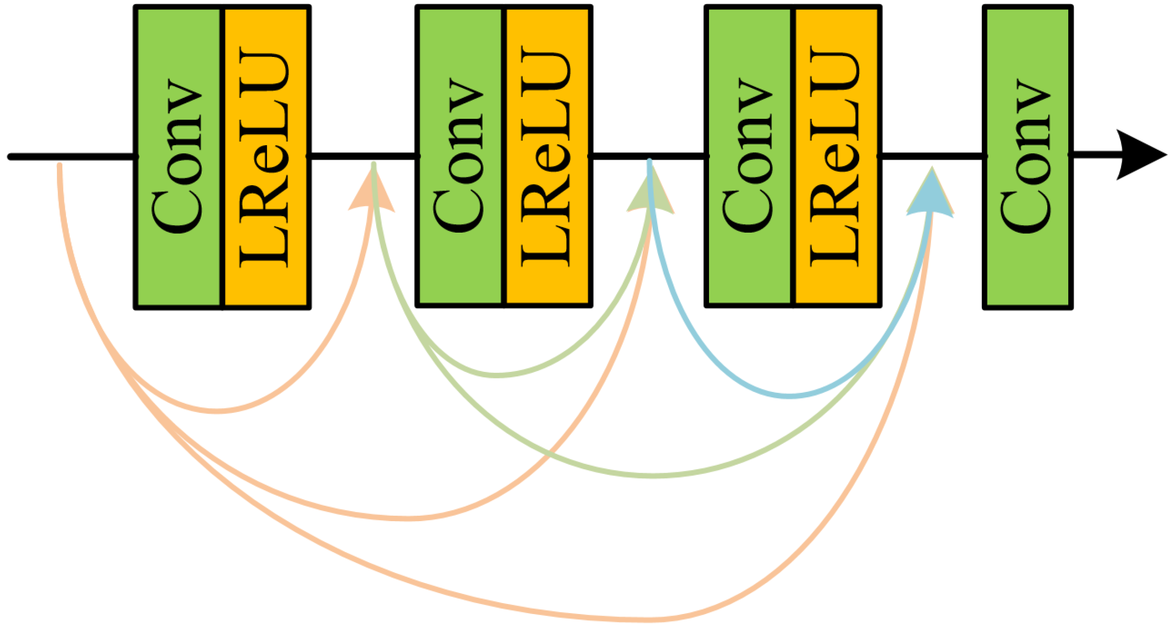
DNCNN [2] uses a convolutional network with a depth of 17 to extract image noise, indicating that noise distribution is easier than image features to be learned by the network. On this basis, a denoising preprocessing method for LR noisy images is proposed. In order to maintain the overall computational complexity of the network, seven convolutional layers to extract the noise distribution in the feature domain are used, as shown in Figure 3. Compared with the original network that only deepened the depth of one dense residual block (RRDB), each layer of the convolutional network adopts the convolution kernel of 3 × 3 and takes the modified linear activation unit (ReLU) as the activation function. Denoising features are obtained by using the residual-skip structure between the original feature and the extracted noise to remove the extracted noise distribution, where the coefficient of residual-skip is −1.

3.2.2. Gradient Branch

Inspired by SPSR [3], the gradient branch into the traditional GAN-based SR network is introduced to learn the mapping of LR to HR edge images and the quality of reconstruction is improved. SPSR [3] ignores the direction information and fuses the intensity of the horizontal and vertical gradients as the gradient diagram corresponding to the image. SPSR thinks that the intensity information is sufficient to reflect the sharpness of the image. Similarly, the direction of the gradient is ignored and the intensity of the gradient is just used. However, through comparison, it is found that focusing on the intensity in only two directions will lose the edge details. Therefore, based on SPSR [3], the gradient in the two directions (45°/135°) is introduced additionally as the gradient map in this paper. At the same time, to understand the mapping between the two resolutions, SPSR [3] suggests that gradient images of different resolutions can be converted between images. In order to focus more on the spatial relationship of the contour, the convolution kernel in the direction of 0°, 45°, 90° and 135° is designed so that the obtained edge image is still close to zero for the most part.
Compared with SPSR [3], an additional gradient in the direction of 45°/135° is introduced. The intensity of the gradient in the four directions constitutes the final gradient diagram. The introduction of gradients in the 45° and 135° directions increases the sharpness of the image edges. Gradient branching is an additional constraint introduced by SR reconstruction, and the enhancement of edge sharpness also has a positive effect on SR reconstruction. Figure 4 compares the gradient maps in two directions with those in four directions.
A wealth of structural information is contained in the layers of convolution of the SR branch, including features at different depths. These features are converted into Gradient information at different depths through Gradient block as input and fused under Gradient branch, which restricts the reconstruction of Gradient branch and makes full use of the network parameters of the SR branch. The reconstructed HR gradient diagram is then integrated into the SR branch to guide SR reconstruction. The final reconstructed gradient results of gradient branching will also be used as part of the objective loss function to optimize the network.

3.2.3. SR Branch

As the input of the SR branch, the denoising preprocessing results will significantly reduce the noise amplified by the SR branch compared with the input without preprocessing. The overall network structure of this paper contains the common SR structure and also integrates the edge information. For the former, the dense residual block (RRDB) proposed in ESRGAN [31] is adopted. Moreover, every five RRDB [31] outputs from the SR branch into the gradient branch is incorporated. In order to maintain the overall sensitivity and depth of the network, the last RRDB is removed. For the conventional SR task, the last convolutional reconstruction layer is removed and the output feature is input into the subsequent part. The latter is the SR gradient diagram obtained by the above gradient branching. The fusion block fuses the characteristics of the two branches together to realize the fusion of structural information. Figure 5 shows the Dense block in RRDB use in ESRGAN [31].

3.3. Loss Function

SR loss: Minimum mean square error (MSE) is widely used to measure the difference between two images to minimize the loss function representing the distance between pixels of two images, which will result in the image failing to maintain visual sharpness. However, its property of easy convergence is still adopted in this paper. The above loss function is expressed by Equation (2):
l M S E = E I S R | | G ( I L R ) I H R | | 1 .
G ( . ) stands for generator, I L R stands for LR input, I H R and stands for ground-truth.
The above formula directly optimizes the difference between pixels without improving the image perception quality. The perception loss proposed by [46] extracts features containing semantic information through a pre-trained VGG network [47]. By comparing the distance between the pixels of the feature map, the result is often satisfactory, as Equation (3):
l S R V G G = E I S R | | Q ( G ( I L R ) ) Q ( I H R ) | | 1 .
Q ( . ) donates the i th layer output of the VGG model.
The original intention of GAN network design is to rely on the game between the generator and discriminator to improve the performance of the network. For the generator, the following objective function is used:
l S R G = E I S R [ log D I ( G ( I L R ) ) ] .
D I represents the discriminator’s judgment of the generated image.
Gradient loss: In order to introduce an edge constraint in image recovery, the gradient loss is represented by the distance between the gradient diagram extracted from the SR image and the gradient diagram extracted from the corresponding HR image.
l M S E G r a d = E I S R | | G r a d ( G ( I L R ) ) G r a d ( I H R ) | | 1 .
G r a d ( . ) stands for the function extracting gradient map.
As a part of GAN, the adversarial loss of the gradient is also a part of the overall objective function:
[ l S R G G r a d = E I S R [ log D G r a d ( G r a d ( G ( I L R ) ) ) ] .
D G r a d is the judgment of the generated image gradient.
Overall loss: All the above are the target functions of the generator. The discriminator has the following form on the SR branch and gradient branch:
l S R D i s = E I S R [ log ( 1 D I ( I S R ) ) ] E I H R [ log ( D I ( I H R ) ) ] , l G r a d D i s = E I S R [ log ( 1 D G r a d ( G r a d ( I S R ) ) ) ] E I H R [ log ( D G r a d ( G r a d ( I H R ) ) ) ] .
For the generator of the SR branch, two parts of the loss are used to supervise the generation of the images. For gradient branching, pixelwise loss l G r a d M S E is used. The loss functions of each part in the SR branch and gradient branch constitute the final generator objective function:
l G = l M S E + α V G G l S R V G G + α G l S R G + β M S E l M S E G r a d + β G l S R G G r a d + γ l G r a d M S E .
α V G G , α G , β M S E , β G and γ are the weights of different loss functions in the total loss function. Among these, the α and the β represent the constraints of the SR branch on the SR image and SR gradient image respectively. The γ donates the weight of the gradient branch loss in the total objective function.

4. Experimental Settings

In order to evaluate the effectiveness of the proposed SNS method, the DIV2K is used as the training set and four common benchmarks are used as the test: Set5 [48], Set14 [49], BSD100 [34] and Urban100 [50]. The LR images are obtained by sampling the HR images with bicubic interpolation and the sampling factor of four is only considered. The noise image is obtained by adding noise to the LR image. The intensity of the added noise is expressed as σ , which is composed of Gaussian noise, salt and pepper noise and Poisson noise. Take the noise with noise intensity σ as an example, including Gaussian noise with intensity σ , pepper and salt noise with intensity σ *0.01 and Poisson noise with intensity σ . Perceptual Index (PI) [50], Learned Perceptual Image Patch Similarity (LPIPS) [51], PSNR and Structure Similarity (SSIM) [52] are selected as the evaluation metrics. Lower PI and LPIPS values indicate higher perceptual quality. The SR branch which borrows from ESRGAN’s architecture and RRDB [31] is used as the Grad Block. The noise is added to the LR images through the function in Matlab and the noise intensities are used to measure the noise level. Because it is difficult to train the GAN and the loss function is difficult to converge, a small change will have a significant impact on the results of the network. So in the actual training process, the MSE as the loss function for pre-training and the parameters obtained from pre-training as the initial value of the network for training are still used. In the training, 16 pairs of matching images as training data for each small batch are applied. MSE is set as the loss function in the pre-training, and the training times are set as 400,000 times, the initial learning rate is 0.0001 and the learning rate decreases by 1/10 at 200,000 times. The α V G G and α G are set as 0.01 and 0.005, respectively, by referring to the weight setting of the loss function in SPSR. For the edge loss introduced later, β M S E and β G are also set as 0.01 and 0.005, respectively. To optimize the gradient branch generation function, the = 0.5 is used. In the actual training process, the training times are set as 200,000, the initial learning rate is also 0.0001, and the learning rate decreases to 1/10 when the training rate reaches 100,000 times. Generally, the model will be converged. All the experiments are implemented by Tensorflow on two pieces of NVIDIA GTX 1080Ti GPUs.

5. Result Analysis

5.1. Quantitative Comparison

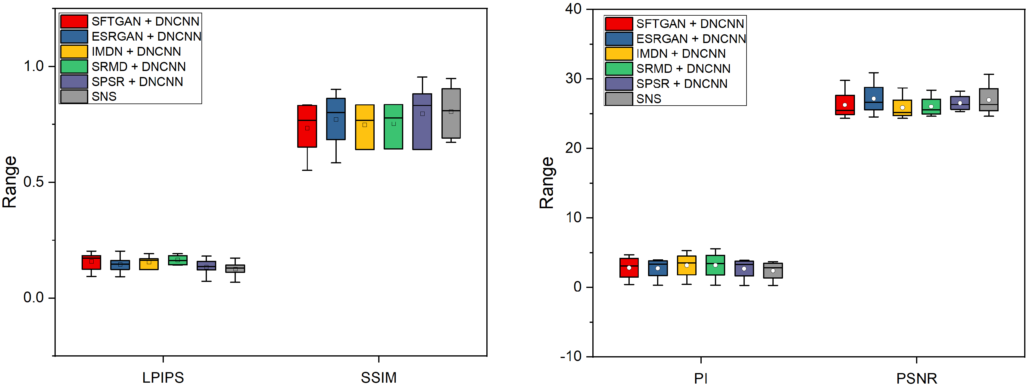
The model used in this article was trained on the equipment we used for about 45 h. This paper focus on the SR task of noisy images, and the denoising preprocessing in the SNS refers to DNCNN [2]. Therefore, the noisy images are preprocessed through DNCNN [2] before comparing with state-of-the-art SR methods, such as SFTGAN [53], ESRGAN [31], IMDN [46], SRMD [47] and SPSR [3]. It should be noted that SNS is not preprocessed by DNCNN [2]. The data in Table 1 are calculated when the noise intensity is 25. This paper artificially adds Gaussian noise, salt-and-pepper noise and Poisson noise to the images. In each row, the best results are highlighted in red and the second best ones are highlighted in blue. It can be seen that SNS achieves the best PI [51] and LPIPS [52] performance for noisy images in all test data sets. At the same time, the values of this paper for PSNR and SSIM [53] in most data sets are close to the best results. In addition, in the SR branch, the denoising preprocessing module designed by this research only adds limited network parameters, which means SNS has better performance than SPSR and ESRGAN in noisy images. In order to measure the performance of the proposed method on different data sets with different noise intensity, the indexes of each method under different datasets with different noise intensity are presented by the box-whisker diagram. For the sake of scale, we put four indicators in two pictures. Lower PI [51] and LPIPS [52] values indicate higher perceptual quality. It can be seen in Figure 6 that under different data sets and noise intensity, the proposed method still achieves the performance of the state-of-the-art stepwise method. Therefore, the results show that the SNS method has the superior ability of less distortion while obtaining good perception quality for noisy images.

5.2. Qualitative Comparison

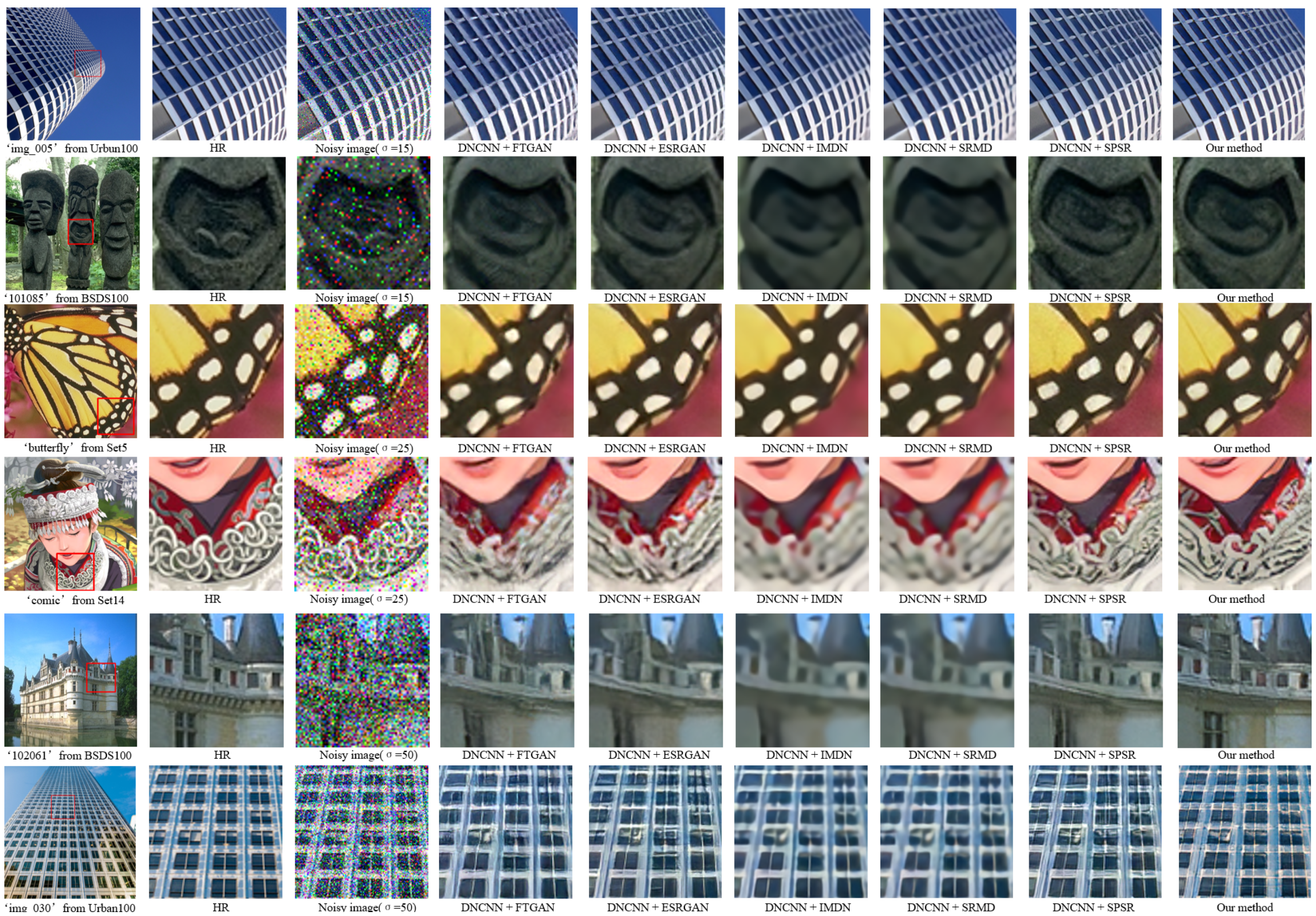
The proposed SNS is visually compared with the state-of-the-art SR approach. For the general SR network, we remove noise through DNCNN [2] while SNS processes the noisy image end to end. As shown in Figure 7, the results of this paper are more natural and realistic than the other two-step approach. The experiment is divided into three groups according to the added noise intensity, which are 15, 25, and 50, respectively. In the first image with a noise intensity of 50, the SNS correctly calculated the shape of the window, indicating that SNS could eliminate the noise in the LR image and capture the structural features of the object in the image. At other noise levels, SNS also recovers better textures than the step-by-step SR method. In our results, the noise is completely removed while the distortion free structure is preserved, while other methods cannot display satisfactory appearance objects. The gradient mapping of the image from Set14 is shown in Figure 8. It can be found that the proposed SNS method has minimal structural degradation compared with other methods. The qualitative comparison shows that the proposed SNS method can obtain more structural information from gradient space after denoising pretreatment and generate realistic SR images by preserving the geometric structure.

5.3. Denoising Preprocessing

SNS is designed for the SR of noisy images, so the denoising preprocessing is added on the basis of SPSR [3]. The denoising preprocessing can perform the initial filtering of the noise before the SR branch. As shown in Figure 9, it is found that the denoising preprocessing has a significant effect on the SR of the noise-containing image. In the process of SR, the noise in the image leads to the wrong mapping, making the result extremely fuzzy.

6. Conclusions

In conclusion, this paper proposes a noisy image SR method, which includes a denoising preprocessing module and a gradient branch. Compared with the stepwise denoising method and SR method, SNS has better perception quality and smaller geometric distortion. Combining different data sets and different noise intensity, compared with the advanced stepwise method, the proposed method improves the performance of the PI index by 17%, LPIPS by 11%, PSNR and SSIM by 5% and 6%, respectively. In the generator, we use multiple convolutional layers to learn the noise distribution, which is removed by residual-skip. The introduced gradient branch combines the edge information of the image as a new constraint with the original spatial constraint to improve the quality of the reconstruction of the noisy image. In future work, this research hopes to design a general-purpose lightweight network model for multi-scale SR that can be used on mobile devices.

Author Contributions

S.H., M.C. and X.Z. propose the conception and design. S.H. conduct the data collection. S.H., M.C., X.Z. and G.C. conduct the data analysis and interpretation. S.H. and M.C. write the original draft. X.Z., M.C. and S.H. make the critical revision. All authors have read and agreed to the published version of the manuscript.

Funding

This work was financially supported by the University of Shanghai for Science and Technology (USST) and National Key Scientific Apparatus Development of Special Item of China (Project Number: 2016YFF0101400).

Conflicts of Interest

The authors declare that they have no known competing financial interests or personal relationships that could have appeared to influence the work reported in this paper.

References

  1. Goodfellow, I.J.; Pouget-Abadie, J.; Mirza, M.; Xu, B.; Warde-Farley, D.; Ozair, S.; Courville, A.; Bengio, Y. Generative Adversarial Nets. In Advances in Neural Information Processing Systems 27; Neural Information Processing Systems Foundation, Inc.: San Diego, CA, USA, 2014. [Google Scholar]
  2. Zhang, K.; Zuo, W.M.; Chen, Y.J.; Meng, D.Y.; Zhang, L. Beyond a Gaussian Denoiser: Residual Learning of Deep CNN for Image Denoising. IEEE Trans. Image Process. 2007, 26, 3142–3155. [Google Scholar] [CrossRef] [PubMed] [Green Version]
  3. Ma, C.; Rao, Y.; Cheng, Y.; Chen, C.; Lu, J.; Zhou, J. Structure-Preserving Super Resolution with Gradient Guidance. arXiv, 2020; arXiv:2003.13081. [Google Scholar]
  4. Hwang, H.; Haddad, R.A. Adaptive median filters: New algorithms and results. IEEE Trans. Image Process. 1995, 4, 499–502. [Google Scholar] [CrossRef] [PubMed] [Green Version]
  5. Zhang, P.X.; Li, F. A New Adaptive Weighted Mean Filter for Removing Salt-and-Pepper Noise. IEEE Signal Process. Lett. 2014, 21, 1280–1283. [Google Scholar] [CrossRef]
  6. Liu, L.; Chen, C.P.; Zhou, Y.; You, X. A new weighted mean filter with a two-phase detector for removing impulse noise. Inf. Sci. 2015, 315, 1–16. [Google Scholar] [CrossRef]
  7. Kandemir, C.; Kalyoncu, C.; Toygar, Ö. A weighted mean filter with spatial-bias elimination for impulse noise removal. Dig. Signal Process. 2015, 46, 164–174. [Google Scholar] [CrossRef]
  8. Zhou, Z. Cognition and Removal of Impulse Noise With Uncertainty. IEEE Trans. Image Process. 2012, 21, 3157–3167. [Google Scholar] [CrossRef]
  9. Li, Z.; Tang, K.; Cheng, Y.; Chen, X.; Zhou, C. Modified Adaptive Gaussian Filter for Removal of Salt and Pepper Noise. KSII Trans. Internet Inf. Syst. 2015, 9, 2928–2947. [Google Scholar] [CrossRef]
  10. Nasri, M.; Saryazdi, S.; Nezamabadi-pour, H. A Fast Adaptive Salt and Pepper Noise Reduction Method in Images. Circ. Syst. Signal Pr. 2013, 32, 1839–1857. [Google Scholar] [CrossRef]
  11. Huang, Y.; Zhang, Y.; Li, N.; Chambers, J. A robust Gaussian approximate filter for nonlinear systems with heavy tailed measurement noises. In Proceedings of the 2016 IEEE International Conference on Acoustics, Speech and Signal Processing (ICASSP), Shanghai, China, 20–25 March 2016; pp. 4209–4213. [Google Scholar]
  12. Jain, V.; Seung, H.S. Natural image denoising with convolutional networks. In Proceedings of the 21st International Conference on Neural Information Processing Systems, Vancouver, BC, Canada, 3–6 December 2007; pp. 769–776. [Google Scholar]
  13. Burger, H.C.; Schuler, C.J.; Harmeling, S. Image denoising: Can plain neural networks compete with BM3D? In Proceedings of the 2012 IEEE Conference on Computer Vision and Pattern Recognition, Providence, RI, USA, 16–21 June 2012; pp. 2392–2399. [Google Scholar]
  14. He, K.; Zhang, X.; Ren, S.; Sun, J. Deep Residual Learning for Image Recognition. In Proceedings of the 2016 IEEE Conference on Computer Vision and Pattern Recognition (CVPR), Las Vegas, NV, USA, 27–30 June 2016; pp. 770–778. [Google Scholar]
  15. Lehtinen, J.; Munkberg, J.; Hasselgren, J.; Laine, S.; Karras, T.; Aittala, M.; Aila, T. Noise2Noise: Learning Image Restoration without Clean Data. arXiv, 2018; arXiv:1803.04189. [Google Scholar]
  16. Chen, J.W.; Chen, J.W.; Chao, H.Y.; Yang, M. Image Blind Denoising With Generative Adversarial Network Based Noise Modeling. In Proceedings of the 2018 IEEE/CVF Conference on Computer Vision and Pattern Recognition, Salt Lake City, UT, USA, 18–23 June 2018; pp. 3155–3164. [Google Scholar] [CrossRef]
  17. Chowdhuri, D.; Sendhil, K.K.S.; Babu, M.R.; Reddy, C.P.J.I.J.o.C.S.; Technologies, I. Very Low Resolution Face Recognition in Parallel Environment. Int. J. Comput. Sci. Inf. Technol. 2012, 3, 4408–4410. [Google Scholar]
  18. Yang, Q.; Yang, R.; Davis, J.; Nister, D. Spatial-Depth Super Resolution for Range Images. In Proceedings of the 2007 IEEE Conference on Computer Vision and Pattern Recognition, Minneapolis, MN, USA, 17–22 June 2007; pp. 1–8. [Google Scholar]
  19. Nasrollahi, K.; Moeslund, T.B. Super-resolution: A comprehensive survey. Mach. Vis. Appl. 2014, 25, 1423–1468. [Google Scholar] [CrossRef] [Green Version]
  20. Ni, K.S.; Nguyen, T.Q. An Adaptable k-Nearest Neighbors Algorithm for MMSE Image Interpolation. IEEE Trans. Image Process. 2009, 18, 1976–1987. [Google Scholar] [CrossRef] [PubMed]
  21. Gribbon, K.T.; Bailey, D.G. A novel approach to real-time bilinear interpolation. In Proceedings of the DELTA 2004 Second IEEE International Workshop on Electronic Design, Test and Applications, Perth, Australia, 28–30 January 2004; pp. 126–131. [Google Scholar]
  22. Fritsch, F.; Carlson, R. Monotone Piecewise Cubic Interpolation. SIAM J. Numer. Anal. 1980, 17, 238–246. [Google Scholar] [CrossRef]
  23. Flowerdew, R.; Green, M.; Kehris, E. Using areal interpolation methods in geographic information systems. Pap. Reg. Sci. 1991, 70, 303–315. [Google Scholar] [CrossRef]
  24. Dong, C.; Loy, C.C.; Tang, X.O. Accelerating the Super-Resolution Convolutional Neural Network. In Proceedings of the Computer Vision—ECCV 2016: 14th European Conference, Amsterdam, The Netherlands, 11–14 October 2016; pp. 391–407. [Google Scholar] [CrossRef] [Green Version]
  25. Shi, W.Z.; Caballero, J.; Huszar, F.; Totz, J.; Aitken, A.P.; Bishop, R.; Rueckert, D.; Wang, Z.H. Real-Time Single Image and Video Super-Resolution Using an Efficient Sub-Pixel Convolutional Neural Network. In Proceedings of the 2016 Ieee Conference on Computer Vision and Pattern Recognition (Cvpr) 2016, Las Vegas, NV, USA, 27–30 June 2016; pp. 1874–1883. [Google Scholar] [CrossRef] [Green Version]
  26. Kim, J.; Lee, J.K.; Lee, K.M. Accurate Image Super-Resolution Using Very Deep Convolutional Networks. In Proceedings of the 2016 IEEE Conference on Computer Vision and Pattern Recognition (Cvpr) 2016, Las Vegas, NV, USA, 27–30 June 2016; pp. 1646–1654. [Google Scholar] [CrossRef] [Green Version]
  27. Kim, J.; Lee, J.K.; Lee, K.M. Deeply-Recursive Convolutional Network for Image Super-Resolution. In Proceedings of the 2016 IEEE Conference on Computer Vision and Pattern Recognition (Cvpr) 2016, Las Vegas, NV, USA, 27–30 June 2016; pp. 1637–1645. [Google Scholar] [CrossRef] [Green Version]
  28. Tai, Y.; Yang, J.; Liu, X.M. Image Super-Resolution via Deep Recursive Residual Network. In Proceedings of the 30th IEEE Conference on Computer Vision and Pattern Recognition (Cvpr 2017), Honolulu, HI, USA, 21–26 July 2017; pp. 2790–2798. [Google Scholar] [CrossRef]
  29. Tong, T.; Li, G.; Liu, X.J.; Gao, Q.Q. Image Super-Resolution Using Dense Skip Connections. In Proceedings of the 2017 IEEE International Conference on Computer Vision (ICCV), Venice, Italy, 22–29 October 2017; pp. 4809–4817. [Google Scholar] [CrossRef]
  30. Wang, X.; Yu, K.; Wu, S.; Gu, J.; Liu, Y.; Dong, C.; Change Loy, C.; Qiao, Y.; Tang, X. ESRGAN: Enhanced Super-Resolution Generative Adversarial Networks. arXiv, 2018; arXiv:1809.00219. [Google Scholar]
  31. Hu, X.; Mu, H.; Zhang, X.; Wang, Z.; Tan, T.; Sun, J. Meta-SR: A Magnification-Arbitrary Network for Super-Resolution. arXiv, 2019; arXiv:1903.00875. [Google Scholar]
  32. Wang, W.; Guo, R.; Tian, Y.; Yang, W. CFSNet: Toward a Controllable Feature Space for Image Restoration. In Proceedings of the 2019 IEEE/CVF International Conference on Computer Vision (ICCV), Seoul, Korea, 27 October–2 November 2019; pp. 4139–4148. [Google Scholar]
  33. Martin, D.; Fowlkes, C.; Tal, D.; Malik, J. A database of human segmented natural images and its application to evaluating segmentation algorithms and measuring ecological statistics. In Proceedings of the Eighth IEEE International Conference on Computer Vision, Vancouver, BC, Canada, 7–14 July 2001; pp. 416–423. [Google Scholar] [CrossRef] [Green Version]
  34. Singh, A.; Porikli, F.; Ahuja, N. Super-resolving Noisy Images. In Proceedings of the 2014 IEEE Conference on Computer Vision and Pattern Recognition, Columbus, OH, USA, 23–28 June 2014; pp. 2846–2853. [Google Scholar]
  35. Laghrib, A.; Ezzaki, M.; El Rhabi, M.; Hakim, A.; Monasse, P.; Raghay, S. Simultaneous deconvolution and denoising using a second order variational approach applied to image super resolution. Comput. Vis. Image Underst. 2018, 168, 50–63. [Google Scholar] [CrossRef] [Green Version]
  36. Hu, J.; Wu, X.; Zhou, J.L. Noise robust single image super-resolution using a multiscale image pyramid. Signal Process 2018, 148, 157–171. [Google Scholar] [CrossRef]
  37. Chen, L.; Dan, W.; Cao, L.J.; Wang, C.; Li, J. Joint Denoising and Super-Resolution via Generative Adversarial Training. In Proceedings of the 2018 24th International Conference on Pattern Recognition (ICPR), Beijing, China, 20–24 August 2018; pp. 2753–2758. [Google Scholar]
  38. Anoosheh, A.; Sattler, T.; Timofte, R.; Pollefeys, M.; Van Gool, L. Night-to-Day Image Translation for Retrieval-based Localization. In Proceedings of the 2019 International Conference on Robotics and Automation (ICRA), Montreal, QC, Canada, 20–24 May 2019; pp. 5958–5964. [Google Scholar]
  39. Luan, F.J.; Paris, S.; Shechtman, E.; Bala, K. Deep Photo Style Transfer. In Proceedings of the 30th Ieee Conference on Computer Vision and Pattern Recognition (Cvpr 2017), Honolulu, HI, USA, 21–26 July 2017; pp. 6997–7005. [Google Scholar] [CrossRef] [Green Version]
  40. Fattal, R. Image upsampling via imposed edge statistics. ACM Trans. Graph. 2007, 26. [Google Scholar] [CrossRef]
  41. Yan, Q.; Xu, Y.; Yang, X.K.; Nguyen, T.Q. Single Image Superresolution Based on Gradient Profile Sharpness. IEEE Trans. Image Process. 2015, 24. [Google Scholar] [CrossRef]
  42. Sun, J.; Sun, J.; Xu, Z.B.; Shum, H.Y. Gradient Profile Prior and Its Applications in Image Super-Resolution and Enhancement. IEEE Trans. Image Process. 2011, 20, 1529–1542. [Google Scholar] [CrossRef] [PubMed]
  43. Liu, Y.; Zheng, C.W.; Zheng, Q.; Yuan, H.L. Removing Monte Carlo noise using a Sobel operator and a guided image filter. Vis. Comput. 2018, 34, 589–601. [Google Scholar] [CrossRef]
  44. Yang, W.H.; Feng, J.S.; Yang, J.C.; Zhao, F.; Liu, J.Y.; Guo, Z.M.; Yan, S.C. Deep Edge Guided Recurrent Residual Learning for Image Super-Resolution. IEEE Trans. Image Process. 2017, 26, 5895–5907. [Google Scholar] [CrossRef] [Green Version]
  45. Bevilacqua, M.; Roumy, A.; Guillemot, C.; Morel, M.L.A. Low-Complexity Single-Image Super-Resolution based on Nonnegative Neighbor Embedding. In Proceedings of the British Machine Vision Conference, Surrey, UK, 3–7 September 2012. [Google Scholar] [CrossRef] [Green Version]
  46. Hui, Z.; Gao, X.B.; Yang, Y.C.; Wang, X.M. Lightweight Image Super-Resolution with Information Multi-distillation Network. In Proceedings of the 27th Acm International Conference on Multimedia (Mm’19), Nice, France, 21–25 October 2019; pp. 2024–2032. [Google Scholar] [CrossRef] [Green Version]
  47. Zhang, K.; Zuo, W.; Zhang, L. Learning a Single Convolutional Super-Resolution Network for Multiple Degradations. In Proceedings of the 2018 IEEE/CVF Conference on Computer Vision and Pattern Recognition, Salt Lake City, UT, USA, 18–23 June 2018; pp. 3262–3271. [Google Scholar] [CrossRef] [Green Version]
  48. Zeyde, R.; Elad, M.; Protter, M. On Single Image Scale-Up Using Sparse-Representations. In Proceedings of the 7th international conference on Curves and Surfaces, Avignon, France, 24–30 June 2010; pp. 711–730. [Google Scholar]
  49. Huang, J.B.; Singh, A.; Ahuja, N. Single Image Super-resolution from Transformed Self-Exemplars. In Proceedings of the 2015 Ieee Conference on Computer Vision and Pattern Recognition (Cvpr), Boston, MA, USA, 7–12 June 2015; pp. 5197–5206. [Google Scholar] [CrossRef]
  50. Blau, Y.; Mechrez, R.; Timofte, R.; Michaeli, T.; Zelnik-Manor, L. The 2018 PIRM Challenge on Perceptual Image Super-resolution. arXiv, 2018; arXiv:1809.07517. [Google Scholar]
  51. Zhang, R.; Isola, P.; Efros, A.A.; Shechtman, E.; Wang, O. The Unreasonable Effectiveness of Deep Features as a Perceptual Metric. In Proceedings of the IEEE Conference on Computer Vision and Pattern Recognition (CVPR), Salt Lake City, UT, USA, 18–23 June 2018; pp. 586–595. [Google Scholar] [CrossRef] [Green Version]
  52. Wang, Z.; Bovik, A.C.; Sheikh, H.R.; Simoncelli, E.P. Image quality assessment: From error visibility to structural similarity. IEEE Trans. Image Process. 2004, 13, 600–612. [Google Scholar] [CrossRef] [Green Version]
  53. Wang, X.T.; Yu, K.; Dong, C.; Loy, C.C. Recovering Realistic Texture in Image Super-resolution by Deep Spatial Feature Transform. In Proceedings of the IEEE Conference on Computer Vision and Pattern Recognition (CVPR), Salt Lake City, UT, USA, 18–23 June 2018; pp. 606–615. [Google Scholar] [CrossRef] [Green Version]
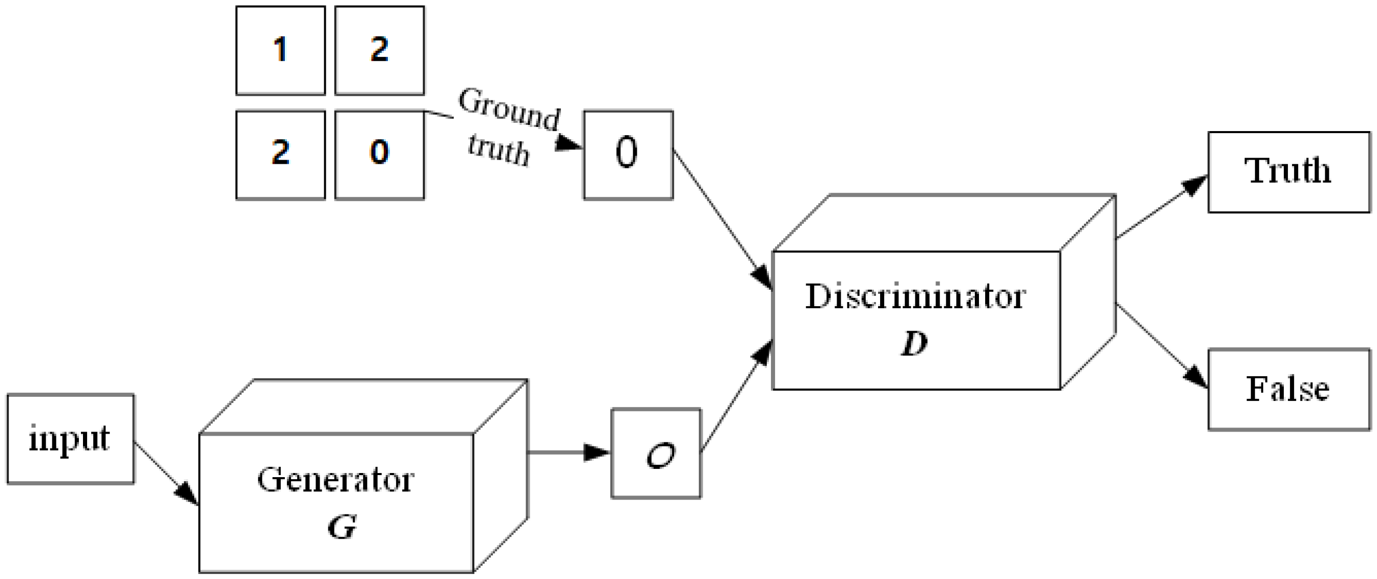
Figure 1. Schematic diagram of generative adversarial network (GAN).
Ai 01 00022 g001
Figure 2. The overall framework of our SNS method.
Ai 01 00022 g002
Figure 3. Denoising preprocessing.
Ai 01 00022 g003
Figure 4. Gradient comparison. From left to right, (a) is ground-truth, (b) is local magnification, (c) is gradient map in two directions and (d) is gradient map in four directions.
Ai 01 00022 g004
Figure 5. The dense residual block (RRDB) used in ESRGAN.
Ai 01 00022 g005
Figure 6. The performance distribution of the proposed method under different data sets and noise intensity.
Ai 01 00022 g006
Figure 7. Comparison of gradient map with state-of-the-art SR methods with denoising preprocessing. The proposed SNS method can better preserve gradients and structures.
Ai 01 00022 g007
Figure 8. Comparison of gradient map with state-of-the-art SR methods with denoising preprocessing. The proposed SNS method can better preserve gradients and structures.
Ai 01 00022 g008
Figure 9. The image of the above row is the SR result of SPSR [3] in the image containing noise without denoising preprocessing, and the second line is the result containing denoising preprocessing.
Ai 01 00022 g009
Table 1. Comparison with advanced super-resolution (SR) networks on benchmark data sets. The best performance is highlighted in red (1st best) and blue (2nd best). The SNS obtains the best PI and LPIPS values as well as the comparable PSNR and SSIM values.
DatasetMetric DNCNN
+SFTGAN
( σ = 15/ σ = 25/ σ = 50)
DNCNN
+ESRGAN
( σ = 15/ σ = 25/ σ = 50)
DNCNN
+IMDN
( σ = 15/ σ = 25/ σ = 50)
DNCNN
+SRMD
( σ = 15/ σ = 25/ σ = 50)
DNCNN
+SPSR
( σ = 15/ σ = 25/ σ = 50)
SNS

( σ = 15/ σ = 25/ σ = 50)
Set5PI5.032/4.712/3.6734.435/3.968/3.6674.823/5.289/5.6735.193/5.573/5.9873.614/3.787/4.0123.023/3.253/3.624
LPIPS0.083/0.093/0.1250.074/0.092/0.1140.103/0.124/0.1340.167/0.184/0.2030.063/0.072/0.0930.053/0.069/0.083
PSNR30.23/29.79/28.4231.26/30.82/29.3229.37/28.72/27.4329.34/28.38/27.5429.64/28.24/27.3431.20/30.65/29.54
SSIM0.905/0.802/0.7230.903/0.863/0.7450.892/0.814/0.7920.883/0.824/0.7630.942/0.832/0.7830.943/0.822/0.733
Set14PI0.343/0.424/0.5340.301/0.325/0.4320.378/0.432/0.5430.295/0.334/0.4230.274/0.303/0.4380.246/0.294/0.405
LPIPS0.132/0.172/0.2340.122/0.137/0.2340.142/0.169/0.2340.132/0.157/0.1670.123/0.138/0.1420.124/0.132/0.141
PSNR26.76/25.52/24.4327.34/26.58/25.2326.85/25.24/24.3426.63/25.83/24.5827.74/26.75/25.3427.47/26.17/25.74
SSIM0.834/0.734/0.6740.837/0.802/0.7390.802/0.723/0.7020.823/0.735/0.6830.892/0.832/0.7340.903/0.793/0.763
BSDS100PI2.432/2.532/3.2342.345/3.059/3.8532.348/3.234/3.7232.345/3.233/3.8342.453/2.972/3.6422.239/2.429/3.032
LPIPS0.123/0.174/0.2630.132/0.157/0.2340.152/0.162/0.2810.143/0.168/0.3020.122/0.158/0.2170.117/0.143/0.202
PSNR26.45/25.41/24.5427.53/26.72/25.4526.45/25.13/24.4526.34/25.31/24.3427.34/25.93/25.3427.83/26.52/25.54
SSIM0.724/0.652/0.5420.762/0.684/0.6130.762/0.642/0.5430.764/0.644/0.5820.749/0.641/0.5580.772/0.672/0.603
Urban100PI3.622/3.642/3.8523.558/3.682/3.7263.578/ 3.782/3.8013.602/3.697/3.7273.501/3.678/3.7693.243/3.527/3.724
LPIPS0.117/0.125/0.1310.118/0.124/0.1380.114/0.123/0.1350.138/0.143/0.1510.119/0.122/0.1280.103/0.112/0.126
PSNR24.57/24.34/24.1224.69/24.55/24.4024.49/24.35/24.2124.71/24.64/24.5025.41/25.32/25.0825.89/24.65/24.03
SSIM0.874/0.834/0.8180.928/0.901/0.8660.857/0.834/0.8220.855/0.836/0.8200.991/0.954/0.9040.923/0.948/0.893