Article

Combining Cirrus and Aerosol Corrections for Improved Reflectance Retrievals over Turbid Waters from Visible Infrared Imaging Radiometer Suite Data

1
Remote Sensing Division, Code 7230, Naval Research Laboratory, Washington, DC 20375, USA
2
Ocean Sciences Division, Code 7330, Naval Research Laboratory, Stennis Space Center, MS 39556, USA
*
Author to whom correspondence should be addressed.
Oceans 2025, 6(2), 28; https://doi.org/10.3390/oceans6020028
Submission received: 26 December 2024 / Revised: 10 March 2025 / Accepted: 6 May 2025 / Published: 14 May 2025
(This article belongs to the Special Issue Ocean Observing Systems: Latest Developments and Challenges)

Abstract

:
The multi-band atmospheric correction algorithms, now referred to as remote sensing reflectance (Rrs) algorithms, have been implemented on a NASA computing facility for global remote sensing of ocean color and atmospheric aerosol parameters from data acquired with several satellite instruments, including the Visible Infrared Imaging Radiometer Suite (VIIRS) on board the Suomi spacecraft platform. These algorithms are based on the 2-band version of the SeaWiFS (Sea-Viewing Wide Field-of-View Sensor) algorithm. The bands centered near 0.75 and 0.865 μm are used for atmospheric corrections. In order to obtain high-quality Rrs values over Case 1 waters (deep clear ocean waters), strict masking criteria are implemented inside these algorithms to mask out thin clouds and very turbid water pixels. As a result, Rrs values are often not retrieved over bright Case 2 waters. Through our analysis of VIIRS data, we have found that spatial features of bright Case 2 waters are observed in VIIRS visible band images contaminated by thin cirrus clouds. In this article, we describe methods of combining cirrus and aerosol corrections to improve spatial coverage in Rrs retrievals over Case 2 waters. One method is to remove cirrus cloud effects using our previously developed operational VIIRS cirrus reflectance algorithm and then to perform atmospheric corrections with our updated version of the spectrum-matching algorithm, which uses shortwave IR (SWIR) bands above 1 μm for retrieving atmospheric aerosol parameters and extrapolates the aerosol parameters to the visible region to retrieve water-leaving reflectances of VIIRS visible bands. Another method is to remove the cirrus effect first and then make empirical atmospheric and sun glint corrections for water-leaving reflectance retrievals. The two methods produce comparable retrieved results, but the second method is about 20 times faster than the spectrum-matching method. We compare our retrieved results with those obtained from the NASA VIIRS Rrs algorithm. We will show that the assumption of zero water-leaving reflectance for the VIIRS band centered at 0.75 μm (M6) over Case 2 waters with the NASA Rrs algorithm can sometimes result in slight underestimates of water-leaving reflectances of visible bands over Case 2 waters, where the M6 band water-leaving reflectances are actually not equal to zero. We will also show conclusively that the assumption of thin cirrus clouds as ‘white’ aerosols during atmospheric correction processes results in overestimates of aerosol optical thicknesses and underestimates of aerosol Ångström coefficients.

1. Introduction

Over 60% of the world’s human population lives in the coastal zone, and it remains the site of the most rapid growth. The growing population affects the coastal ocean through waste disposal, erosion, shipping, fisheries, and military and recreational uses. While it is only 8% of the ocean area, the coastal zone is responsible for about 14% of the global ocean primary production and over 90% of the world’s fish catch. Accurate atmospheric correction over the turbid coastal water is essential to the derivation of water-leaving reflectances and products, such as chlorophyll, phytoplankton primary production, color dissolved organic matter (CDOM), and suspended sediments, from remotely sensed data. A review of the current status and future perspective of satellite ocean color has been given by Groom et al. [1], which emphasized that the user community of satellite ocean color data products needs improved coastal algorithms and data products.
Another review of the history of NASA’s ocean color instrumentation, technology advancement, and algorithm development over the past 40+ years has been given by McClain et al. [2]. For instrumentation, this paper covers from the earlier Coastal Zone Color Scanner (CZCS) (1978–1986), the Sea-viewing Wide Field-of-View Sensor (SeaWiFS) (1997–2010), the Moderate resolution Imaging Spectroradiometer (MODIS) (1999–Present), the Visible-Infrared Imaging Radiometer Suite (VIIRS) (2011–Present), to the current Plankton, Aerosol, Cloud, ocean Ecosystem (PACE) hyperspectral Ocean Color Imager (OCI). For algorithms, this paper has one section on Sensor Intercalibration and Merger for Biological and Interdisciplinary Ocean Studies (SIMBIOS) (1997–2003). The funded researchers through SIMBIOS were obligated to make deliverables to the Project Office at NASA Goddard Space Flight Center. By the time the VIIRS ocean color data products became available, NASA’s ocean color program had made a transition from a pure research focus to a combined research and application focus. The MODIS and VIIRS data products were made publicly available to support not only research in multiple scientific disciplines, but also for routine practical applications by NOAA and the Department of Defense [2].
The easy access to MODIS and VIIRS ocean color (OC) data products through the internet also allowed data users to conduct time series of data analysis. For example, Bisson et al. [3] have identified seasonal bias in NASA’s global ocean color products. They reported that the products derived from the NASA remote sensing reflectance (Rrs) data products were affected by the bias to varying degrees, with particulate backscattering varying up to 50% over a year, chlorophyll concentration varying up to 25% over a year, and absorption from phytoplankton or dissolved material varying by up to 15%. The investigation by Bisson et al. [3] highlights the contributions that atmospheric correction schemes can make in introducing biases in the Rrs data products. They stated that community efforts were needed to find the root cause of the seasonal bias because all the past, present, and future data are, or will be, affected until a solution is implemented. One long-standing issue with NASA’s operational atmospheric correction algorithms was that the high-altitude thin cirrus clouds, typically located approximately 10 km above the earth’s surfaces, were treated as ‘white’ aerosols located at the bottom boundary layer (about 2 km) of the atmosphere in the Rrs retrievals. We inspected monthly mean MODIS cirrus reflectance images, the aerosol optical thickness (AOT) images, and the Angstrom (α) images over the nine Case 1 water areas located in different geographical regions, as illustrated in Figure 5 of Bisson et al. [3]. We observed that AOTs were positively correlated with cirrus reflectances, while α values were negatively correlated with cirrus reflectances. However, the errors in the aerosol data products are unlikely the sources for the seasonal Rrs bias over the 9 Case 1 water areas [4]. Therefore, there is still room for improvement in the Case 1 water atmospheric correction algorithms.
Another issue with publicly available ocean color products is that the products are frequently not retrieved over large portions of oceans, in particular over turbid Case 2 waters, even after the implementation of the iterative approach by Bailey et al. [5] for improved satellite ocean color data processing. Such an example is shown in Figure 1, which is downloaded from a NOAA ocean color web site [6]. The VIIRS RGB image is shown in Figure 1A. The corresponding diffuse attenuation coefficient for the downwelling spectral irradiance at the wavelength 490 nm [7], Kd(490), over Arctic waters is shown in Figure 1B. The VIIRS data were acquired on 19 June 2021. The lower portion of the bright red-colored areas had retrievals. However, over the vast brownish colored turbid waters, ocean color products were not derived. In view of the present global warming situation and the increasing human activities over the Arctic, it is critically important to have timely ocean color data products, such as chlorophyll concentration and water turbidity over Arctic waters.
The ocean color signal is a relatively small part (<10%) of the satellite-measured top-of-atmosphere (TOA) signal over the vast open ocean waters, which justifies the need for very accurate atmospheric correction schemes to retrieve water signals [1]. Over turbid waters or shallow waters with strong reflection from bottom sandy surfaces, such as over the shallow waters in Bahamas Banks, the fraction of water leaving radiances in the visible can be significantly greater than 10% of the TOA satellite measured radiances. The NASA series of OC atmospheric correction algorithms have various built-in masks [8,9], including the cloud mask and glint mask, which stop pixels with a reflectance > 0.027 at 0.865 μm at TOA from being processed. This is too strict and leads to data gaps over very turbid waters, such as those associated with the Río de La Plata in South America and waters off the east coast of China. With proper adjustment in the masking criteria, Rrs retrievals over more bright water areas could be made.
The presence of widespread semi-transparent thin cirrus clouds in the upper part of the atmosphere often complicates the efforts in accurate remote sensing of land surfaces and ocean color. The aforementioned cloud and glint masks used in the NASA OC algorithms often screen out thin cirrus pixels as well as bright water pixels. Through the analysis of Landsat 8, MODIS, and VIIRS data, we demonstrated that ocean color features over bright Case 2 waters contaminated by thin cirrus clouds can be recovered from the remotely sensed data [10,11]. If the thin cirrus scattering effects were first removed and then followed by a normal atmospheric correction process, the remotely sensed OC data products over Case 2 waters would have more extended spatial coverages.
In this paper, we describe a method to combine cirrus corrections and aerosol corrections for increasing spatial coverages of surface reflectances over turbid waters from VIIRS data. In Section 2, we briefly describe the VIIRS cirrus reflectance algorithm [11], the spectrum-matching algorithm [12] for water-leaving reflectance retrievals from the VIIRS data, and the combination of the two algorithms and simplifications made to make fast and stable retrievals. In Section 2, we also describe some of the definitions used in the NASA Rrs algorithm in order to facilitate the comparisons between our algorithm and the NASA Rrs algorithm. In Section 3, we present retrieval results from four VIIRS scenes and compare them with those from the NASA Rrs data products. We give brief discussions in Section 4 and a summary and conclusions in Section 5.

2. Data and Methods

2.1. The VIIRS Instrument

The VIIRS instrument has 11 bands located between the 0.4 and 2.5 μm solar spectral region, as listed in Table 1 and illustrated in Figure 2. The bands are plotted over a reflectance spectrum acquired above a shallow water area with reflection from the sea floor and a TOA reflectance spectrum of a typical cirrus cloud pixel. This shallow water spectrum was selected from field-measured spectra over the coastal area of New Jersey at the Long-term cabled Ecosystem Observatory at 15 m (LEO-15), deployed in 1996. The bands below 1 μm (M1–M7) are illustrated in thick and short green bars. These bands are commonly referred to as visible and near-IR bands (VSNIR) and are used in the NASA VIIRS Rrs algorithm [2,8] for routine processing of VIIRS data. Because the M7 band centered near 0.865 μm can receive solar light scattered by suspended sediments, this band is not ideally suited for retrieving aerosol information from satellite-measured data over turbid coastal waters. The four bands above 1 μm, i.e., M8, M9, M10, and M11, are marked in purple color. These bands are referred to as shortwave IR bands (SWIR). Because liquid water absorption in the ocean above 1 μm is very strong, the water-leaving reflectances of these SWIR bands in coastal waters are often close to zero. The M8, M10, and M11 bands are more suited for atmospheric corrections over turbid water pixels. M9 is located inside a strong atmospheric water vapor band absorption region. This band is now commonly used for thin cirrus detection from satellite images [10,11]. The dominant atmospheric O3 and O2 bands, water vapor bands, and ice bands are also marked in Figure 2.

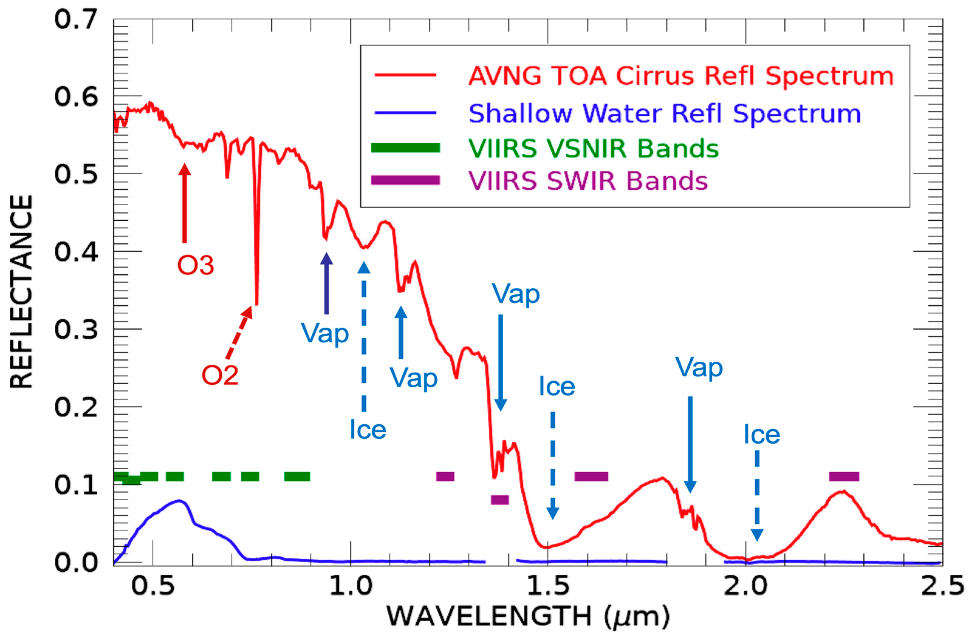
2.2. The VIIRS Cirrus Reflectance Algorithm

The narrow VIIRS M9 band centered at 1.378 μm is specifically designed for remote sensing of cirrus clouds. The images of this band can also be used for quantitative removal of thin cirrus scattering effects from other VIIRS bands located in the 0.4–2.5 μm solar spectral region. The VIIRS cirrus reflectance algorithm was previously reported by Gao and Li [11], which is briefly described here for clarity. The diagram in Figure 3 illustrates atmospheric paths for the M9 solar radiation and another arbitrary VIIRS solar band located in an atmospheric ‘window’ region, where the gas absorption effect is negligible. The algorithm assumes 3 layers above the Earth’s surface, as illustrated in the leftmost portion of Figure 3. The lower layer consists of water clouds (such as cumulus clouds), aerosol, and 90 to 99% of atmospheric water vapor amount from ground to space in a vertical path. The middle is a high cloud (or cirrus cloud) layer typically located at an altitude of approximately 10 km above the Earth’s surface. There is another upper water vapor layer above the cirrus layer. This upper layer typically contains 1 to 10% of vertical column amount of water vapor from ground to space. As illustrated in the right portion of Figure 3, the downward solar radiance near 1.38 μm (in this case M9 band) is slightly absorbed by water vapor above the high cloud layer, reflected and scattered backward, and absorbed by the upper water vapor layer again before reaching the field of view of a satellite sensor. The portion of downward radiance transmitted through the cirrus layer, as illustrated with dashed purple line, is absorbed by vast amount of water vapor beneath cirrus. As a result, the 1.38 μm band detects cirrus clouds against a black background. For the downward solar radiance of an atmospheric window band, as illustrated in the left to middle portion of Figure 3, a small part of it is scattered backward by the cirrus layer. A larger portion is transmitted through the cirrus layer, reaching the bottom surface, reflected and scattered backward, and eventually reaching the satellite sensor’s field of view. Thus, the atmospheric window band receives both the cirrus scattered radiance and the surface reflected radiance. The VIIRS cirrus reflectance algorithm finds the correlations between radiance values of cirrus pixels in the 1.38 μm band image (not affected by the bottom Earth’s surface) and radiance values in the atmospheric window band image (affected by bottom surface) and then makes use of the correlations to estimate the cirrus scattered portions of radiances in the window band image on a pixel by pixel basis. For more details of the algorithm readers are referred to Gao and Li [11].
The VIIRS cirrus reflectance algorithm has been implemented at a VIIRS Atmospheric Sciences computing facility at University of Wisconsin in Madison, Wisconsin, for operational generation of VIIRS cirrus reflectance data products. The SNPP VIIRS cirrus reflectance data products from 1 March 2012 to present are available from a NASA data center. Figure 4 shows an example of cirrus removal over Case 2 waters. Figure 4A is a portion of a VIIRS RGB image acquired on 11 July 2014 over Baltic Sea during a peak chlorophyll blooming event. Figure 4B is the corresponding M9 band cirrus image. The images are highly stretched so that the thin cirrus features can be seen in both images. Figure 4C is the cirrus-removed RGB image. The cirrus features within the area outlined by a red square in Figure 4A,B are removed properly in Figure 4C. The very thin cirrus features in the bottom portion of Figure 4B are also properly removed in Figure 4C image, but the visual effects are less dramatic when comparing Figure 4C image with Figure 4A image, mainly because the cirrus features are optically thin with M9 band reflectance values less than 0.01 (truly ‘sub-visual’ in Figure 4A image).
A concern regarding the cirrus correction algorithm is about the possibility of propagating noise in the M9 band image to VIIRS visible band images. The case study shown in Figure 4 has demonstrated great success in recovering ocean features after the cirrus removal using the M9 band image, which partially addressed this concern. To further quantify the noise level of VIIRS channels, the left and middle panels of Figure 5A show a section of a VIIRS visible RGB image strongly affected by sun glint over the same area of the scene, but for the M9 band, respectively. The filled ‘red square’ is an area free of cirrus clouds. We calculated the means and standard deviations for VIIRS M1–M11 channels over the red square. The standard deviation for the M9 channel in reflectance unit is 0.00016, which is much smaller than the ocean color community’s requirement of noise level at ~0.001 (in reflectance units). As a result, the M9 channel image is usable for the quantitative removal of thin cirrus scattering effects in other VIIRS bands without introducing noticeable noise into cirrus-corrected images. The horizontal stripes in the RGB image in Figure 5 and large local standard deviations for M1–M8 and M10–M11 bands are most likely related to the so-called ‘differential’ polarization sensitivities associated with 16 detectors of a band in the along-track direction. The polarization properties [13] of detectors for VIIRS instrument were well characterized during pre-launch lab calibration. To our understanding, the differential polarization issue in the post-launch VIIRS satellite data has not been fully addressed during radiometric calibration processes. The surface bidirectional reflectance factors may also be contribute to the horizontal stripes.

2.3. Atmospheric Correction Algorithms for Coastal Waters

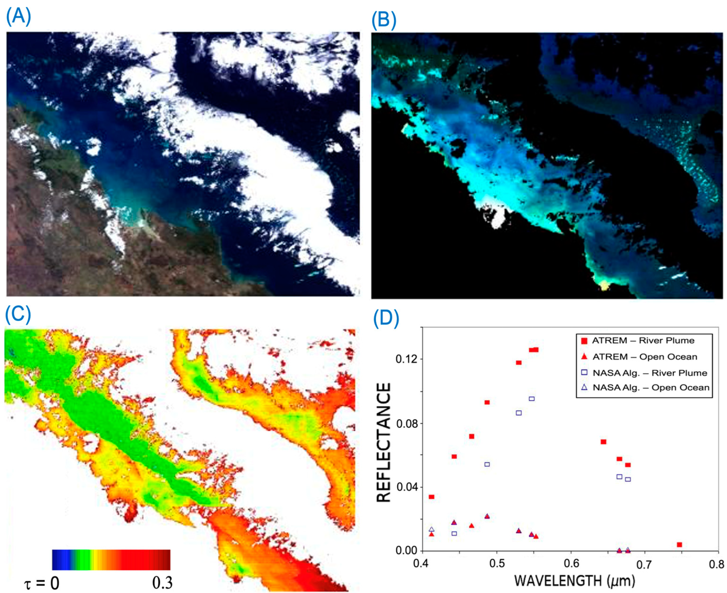
2.3.1. The Development of a Hyperspectral Atmospheric Correction Algorithm

In the late 1990s, we developed an ocean version of the hyperspectral atmospheric correction algorithm [14] for supporting the Navy COIS (Coastal Ocean Imaging Spectrometer) project [15]. At the time, we found that the water-leaving reflectances over turbid coastal waters near 0.75 and 0.86 μm were not close to zero, based on our analysis of available hyperspectral imaging data acquired with the Airborne Visible Infrared Imaging Spectrometer (AVIRIS) [16]. The NASA SeaWiFS atmospheric correction algorithm developed by Gordon and Wang [17], hereafter referred to as GW94, used bands centered near 0.75 and 0.86 μm for aerosol retrievals, which is not ideally suited for processing remotely sensed data acquired over turbid coastal waters. Our analysis of AVIRIS images for bands above 1 μm showed that the SWIR images were nearly black because of strong liquid water absorption above 1 μm. We developed the ocean version of the hyperspectral atmospheric correction algorithm based on the radiative transfer formulation by Fraser et al. [18,19], which uses bands above 1 μm and a spectrum-matching technique for estimating aerosol model and optical thickness, and extrapolated the aerosol information to the visible for the retrieval of water-leaving reflectances of visible bands [14]. The algorithm was applied to multiple AVIRIS data collected over coastal areas of the Gulf of Mexico, Florida, Virginia, Maryland, and New Jersey during various airborne campaigns.
The adoption of the Fraser formulation permits the simultaneous matching of measured radiances of several bands centered at different wavelengths with those from theoretical simulations and results in more stable estimates of aerosol models and optical depths. We used the common definition of apparent reflectance ρ*obs at top-of-atmosphere (TOA) for a given wavelength [14,20], and
ρ*obs = π Lobs/(μo Eo),
where Lobs is the radiance of the ocean–atmosphere system measured by a satellite instrument, μo is the cosine of solar zenith angle, and Eo is the downward solar irradiance at TOA when the solar zenith angle is equal to zero. If we neglect the interactions between atmospheric gaseous absorption and molecular and aerosol scattering, we can express ρ*obs as [14]
ρ*obs = Tg [ρ*atm+sfc + ρw td tu/(1 − s ρw)],
where Tg is the total atmospheric gaseous transmittance on the sun–surface–sensor path, ρ*atm+sfc is the reflectance resulting from scattering by the atmosphere and specular reflection by ocean surface facets, td is the downward transmittance (direct + diffuse), tu is the upward transmittance, s is the spherical albedo that takes account of reflectance of the atmosphere for isotropic radiance incident at its base, and ρw is the water-leaving reflectance.
Solving Equation (2) for ρw yields
ρw = (ρ*obs/Tgρ*atm+sfc)/[td tu + s (ρ*obs/Tgρ*atm+sfc)].
Given a satellite-measured radiance, the water-leaving reflectance can be derived according to Equation (3), provided that the other quantities in the righthand side of Equation (3) can be modeled theoretically. We used a modified version of the Ahmad and Fraser code [21] to generate lookup tables. More specifically, we used the code to generate the quantities ρ*atm+sfc, td, tu, and s in Equation (3). Lookup tables for 14 wavelengths between 0.39 and 2.5 μm in atmospheric “window” regions, sets of aerosol models, optical depths, solar and view angles, and surface wind speeds were generated. Aerosol models similar to those used in the SeaWiFS algorithm, plus additional absorbing aerosol models, were used during the table generation.

2.3.2. The Development of Multi-Band Atmospheric Correction Algorithms

In early 2000s, with financial support from the NASA SIMBIOS Project [2], we successfully modified the existing hyperspectral algorithm for use with multi-band SeaWiFS and MODIS data. The main modification was to speed up the spectrum-matching process. At the time, most hyperspectral scenes covered areas less than 30 km by 30 km. It was a reasonable assumption that the solar and view zenith angles for all pixels within a scene were constants. However, for the wide swath of SeaWiFS and MODIS scenes, the solar and view zenith angles were varying on a pixel-by-pixel basis. It was time-consuming to do spectrum-matching on a pixel-by-pixel basis for aerosol retrievals on available SGI workstations at the time. We had to improve our code in order to be able to process one MODIS scene within about 30 min on a computer with a maximum memory size of 200 megabytes. Although a bit slow, we were able to make retrievals from multiple MODIS data sets using an SGI workstation after performing 10-by-10-pixel spatial averaging for aerosol retrievals.
Figure 6 shows examples of water-leaving reflectance retrievals with algorithm (nicknamed ATREM (Atmosphere REMoval); hereafter, see [22]) and a NASA version of MODIS algorithm, which was a slight variation in the GW94 SeaWiFS algorithm. Figure 6A is a color image processed from a set of MODIS land channels (Red: 0.645 μm; Green: 0.55 μm; Blue: 0.47 μm). The land–water boundaries are in the lower left portion of the scene. The water surface areas near the mouth of a big river appear white-bluish. Figure 6B shows the color image processed from the water-leaving reflectances (for the same three land bands) retrieved with our algorithm. Clouds and land surfaces were masked out in this image. The near-IR and SWIR bands centered at 0.86, 1.24, and 1.64 μm were used for the derivation of aerosol optical thicknesses and aerosol models. From this figure, it is seen that our algorithm allowed the successful derivation of water-leaving reflectances over bright coastal waters. Figure 6C is the aerosol optical thickness image. Figure 6D shows examples of water-leaving reflectances retrieved with our algorithm and with the NASA Rrs algorithm. Over the deep ocean area, the water-leaving reflectances derived with both algorithms agreed quite well. However, over the turbid water area, the water-leaving reflectances between 0.4 and 0.55 μm derived with the NASA algorithm are significantly smaller than those derived with our algorithm. This can be attributed to the fact that, over the turbid water area, the water-leaving reflectance for the 0.75 μm MODIS ocean color channel is not close to zero. The NASA Rrs algorithm assumed zero water-leaving reflectance for this band during the derivation of aerosol optical depths and aerosol models. The algorithm under-estimated the aerosol particle sizes, over-estimated aerosol optical depths, and, therefore, over-estimated atmospheric path reflectances in the visible band after the extraction of aerosol information from NIR to visible band. The subsequent subtraction of path reflectances from the MODIS-measured TOA radiances in reflectance unit resulted in significant underestimates of water-leaving reflectances in the visible spectral region with the NASA Rrs algorithm. Because our MODIS algorithm was funded by the NASA SIMBIOS project [2] through a contract, we delivered the source code along with input and output files to NASA in the summer of 2002 to fulfill the contract requirement. In 2007, several years after the ending of the SIMBIOS, we published a paper on retrieving water-leaving reflectances from MODIS data with our spectrum-matching algorithm [22] using a combination of MODIS land and ocean bands. The use of MODIS land bands for retrieving water-leaving reflectances over coastal waters was necessary because the two MODIS ocean-atmospheric correction bands centered near 0.75 and 0.86 μm were saturated over some bright coastal water pixels. The saturation problems were rectified for the corresponding VIIRS M6 and M7 atmospheric correction bands, as listed in Table 1.
Around 2015, we ported over our hyperspectral atmospheric correction algorithm to process VIIRS data on a scene-by-scene basis. The main tasks were to interpolate pre-calculated atmospheric scattering lookup tables with the Ahmad and Fraser [21] vector radiative transfer code originally for our hyperspectral algorithm [14] into the wavelengths of VIIRS M1–M11 bands and to use the same spectrum-matching scheme implemented in our MODIS algorithm for retrievals from VIIRS data on the pixel by pixel basis. Lookup tables for modeling atmospheric gas transmittances of VIIRS M1–M11 bands were also generated. At the same time, we were funded by NASA to develop an operational VIIRS cirrus reflectance algorithm. Figure 5 illustrates our efforts in objective assessments of the noise of real VIIRS M1–M11 data, including the M9 cirrus band data, in the solar spectral region. We showed that the VIIRS M9 cirrus band had sufficiently good signal-to-noise ratios for use in the quantitative removal of thin cirrus effects in other VIIRS bands and could be used to improve the VIIRS land, ocean, and atmospheric data products if thin cirrus effects were removed during the 2015 MODIS/VIIRS Science Team Meeting [23]. Later on, we improved the 2015 version of VIIRS atmospheric correction algorithm so that retrievals could be made almost automatically for multiple VIIRS scenes in one batch job on a MacBook laptop computer. In 2023, we published a paper on the VIIRS algorithm [12] and demonstrated that increased spatial coverage over turbid waters could be made using VIIRS SWIR bands (M8, M10, M11) and a spectrum-matching technique for aerosol retrievals.
Soon after the publication of the VIIRS atmospheric correction paper, we made careful comparisons between the original lookup tables generated with the 1982 Fraser and Ahmad code in the late 1990s with new lookup tables generated in 2021 with an improved pseudo-spherical shell algorithm for vector radiative transfer (RT) modeling developed by Zhai and Hu [24]. The same Zhai and Hu code has also been used in generating lookup tables [25] for the NASA PACE OCI Rrs algorithm. Through our comparisons for the quantities stored in the lookup tables, such as atmospheric scattered path reflectances downward and upward transmittances generated with the two algorithms with about the same solar and view angles and aerosol models, they agreed quite well (typically within 0.5%). The original lookup tables (based on the Fraser and Ahmad codes) were generated on relatively coarse angular grids (as large as 12° at certain solar and azimuth angle ranges) due to the lack of computing power in late 1990s. The linear interpolation of the quantities stored in the lookup tables sometimes does not produce smooth results in the relevant angular domains. The original tables also do not have UV coverage for bands below 0.39 μm.
The new lookup tables were generated with a wavelength coverage starting from 0.35 μm (UV) and ending at 2.25 μm (SWIR) in 18 bands, at a fine angular grid spacing of 6° for solar zenith, view zenith, relative azimuth angles, three surface wind speeds (2, 6, and 10 m/s), and a black bottom surface without any reflection. Additional absorbing aerosol models and non-spherical dust aerosol models were also constructed and used in the generation of the new lookup tables. The new lookup tables are better suited for solar and view zenith angles greater than 75° in view of the improved pseudo-spherical shell algorithm for RT modeling. In our present spectrum-matching version of VIIRS algorithm, we have replaced the original lookup tables with the new tables simulated with Zhai and Hu radiative transfer code [24].

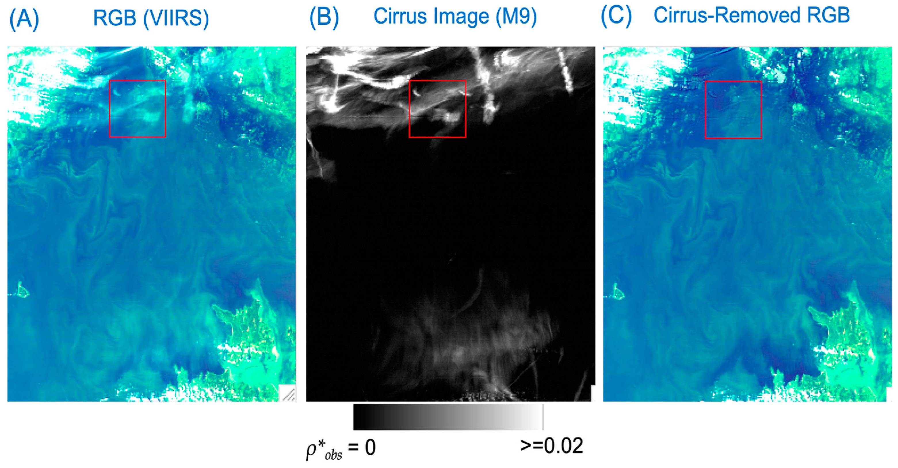
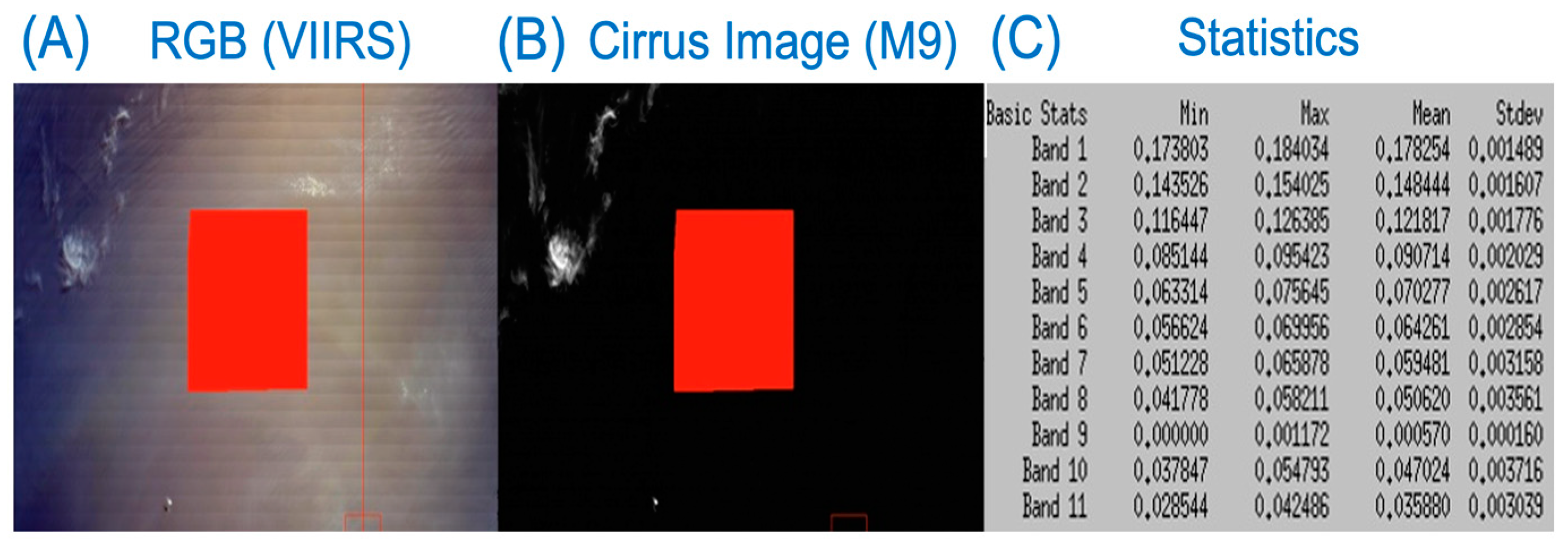
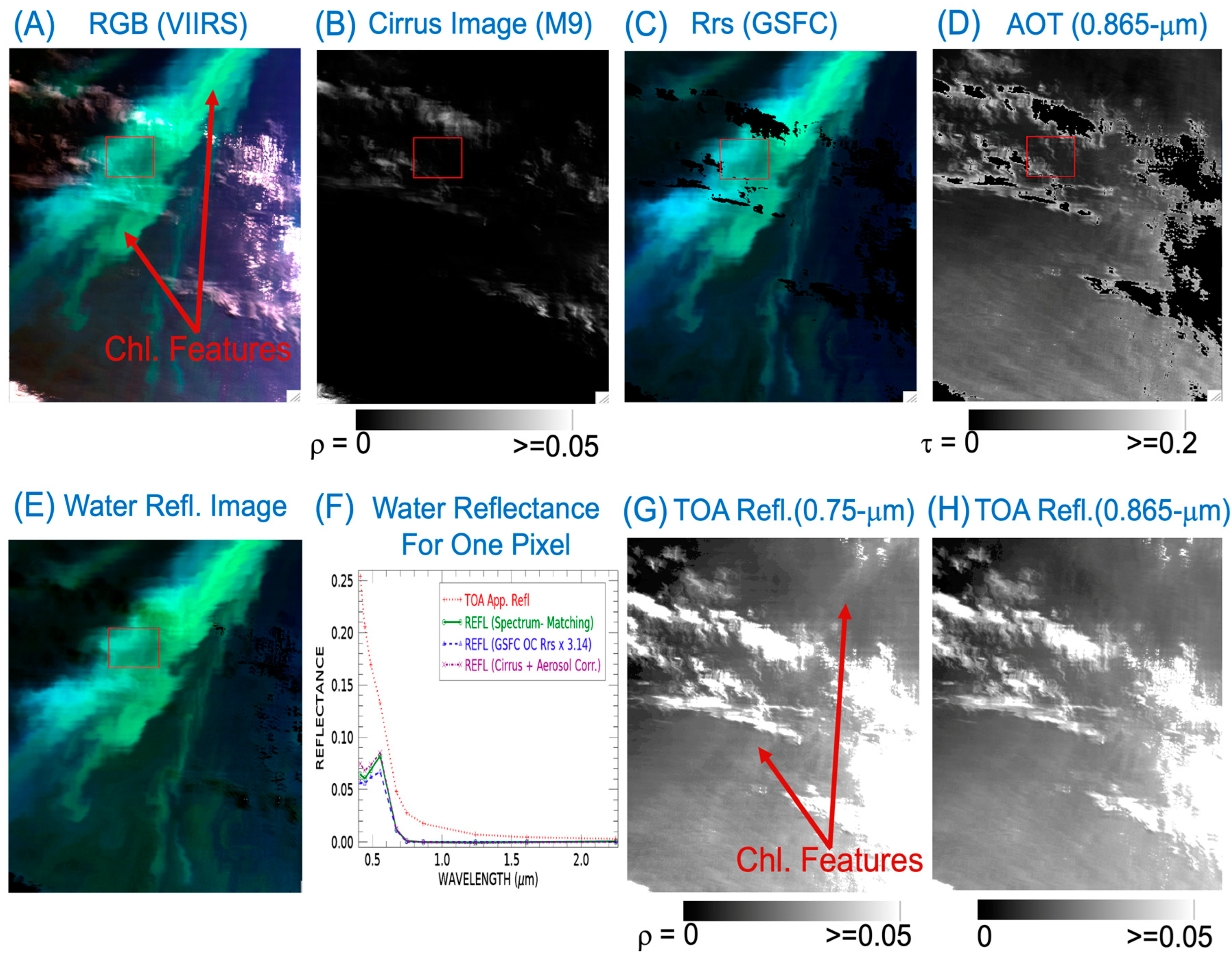
2.3.3. Combining Cirrus and Aerosol Corrections for Improved Retrieval of Turbid Water Reflectances

Thin cirrus clouds are widely distributed in the world. The global and seasonal distribution of cirrus clouds based on satellite lidar measurements were reported by Nazaryan et al. [26]. It is common that the cirrus fraction over a geographic region is 30% or greater. For a VIIRS atmospheric window band, as illustrated in Figure 3, the downward solar radiance is first scattered back by cirrus clouds to the satellite sensor. This cirrus-induced atmospheric path radiance does not contain information about the lower atmosphere or the land and water surfaces below the cirrus. Additionally, the multiple reflection and scattering effects between thin cirrus clouds and the lower atmosphere–surface system are generally small. Natural thinking for atmospheric corrections is to first remove the upper-level thin cirrus scattering effects and then perform normal atmospheric corrections when retrieving information about the lower-level aerosols and surface reflectances. In reality, most current atmospheric correction algorithms do not make explicit cirrus removals but only treat thin cirrus clouds as aerosols.
As early as 2002, we noticed problems with the NASA SeaWiFS and MODIS aerosol data products [27]. We reported that AOTs over areas near Hawaii in the Pacific Ocean from SeaWiFS data were as large as 0.6, which was significantly greater than those inferred from ground-based upward-looking sun photometers (~0.1). We stated in [27] that the thin cirrus contamination was identified as the main source for the overestimation of AOTs and underestimation of Angstrom coefficients from SeaWiFS data. At the time, the MODIS aerosol AOT values were also grossly overestimated due to thin cirrus contamination. We suggested to the MODIS aerosol algorithm developers that they should do cirrus corrections followed by a normal aerosol retrieving process. The suggestion was not accepted. Instead, the MODIS aerosol algorithm developers agreed only to have an improved cirrus masking with the method described in [27]. In the 2002 version of MODIS aerosol algorithm and subsequent updated algorithms, however, MODIS pixels with the 1.375 μm cirrus band’s TOA reflectance values less than about 0.02 are all treated as ‘clear’ pixels during aerosol retrievals. The corresponding maximum error in AOTs for a pixel due to cirrus contaminations is approximately 0.2 (0.02 × 10), which is greater than the global AOT climatological value of about 0.1.
In order to avoid the common problem of misprocessing the upper-level thin cirrus clouds as the low-level aerosols during atmospheric correction, we decided to combine the cirrus correction and aerosol correction for water-leaving reflectance retrievals from VIIRS data. We first retrieved VIIRS cirrus reflectances using the method described in Section 2.2. We then subtracted out the retrieved cirrus reflectance values from the VIIRS TOA reflectances for VIIRS M1–M8 and M10–M11 bands. Further on, we used the updated spectrum-matching version of VIIRS algorithm described near the end of Section 2.3.2 to retrieve water-leaving reflectances from the cirrus-removed VIIRS data. This combined cirrus and aerosol correction algorithm is hereafter referred to as ATREMmatch, where ‘ATREM’ stands for ‘ATmosphere REMoval’, and ‘match’ for ‘spectrum-match’. Such combined retrievals were made for 50 selected VIIRS scenes acquired over different geographic regions. To process one VIIRS scene with ATREMmatch, it typically took approximately 30 min on a MacBook pro computer with an Intel I9 processor. Because the spectrum-matching process was slow, we also tried to use a simplified method to make VIIRS water-leaving reflectance retrievals.
The simplified method is based on several factors. One factor is that over turbid waters or shallow waters with strong reflection from the ocean floor, the fraction of water leaving radiances in the visible is significantly greater than 10% of the TOA satellite measured radiances. As a result, more errors can be tolerated for atmospheric corrections over turbid waters. Another factor is that the global AOT values for aerosols over both land and ocean are only about 0.1. As early as the early 1990s, researchers [28] were able to retrieve reliable multi-band land surface reflectances from Landsat 5 TM data, assuming a climatological aerosol model with an AOT of 0.1 and using simulation results with a radiative transfer code. The third factor is that atmospheric aerosols have self-compensating effects between absorption and scattering, as reported in a 1985 landmark paper on aerosol retrievals by Fraser and Kaufman [29]. At a critical surface reflectance value for a band, the increasing or decreasing of AOTs does not change the TOA reflectance of the band. The fourth factor is that the sunglint effects for a given pixel are nearly spectrally constant. To a first-order approximation, the wavelength dependence of sunglint effects can be neglected.
With consideration of these practical factors, our simplified water-leaving reflectance retrieving procedures are as follows. Cirrus reflectances are removed from the TOA reflectances for VIIRS bands. Atmospheric corrections are made on a pixel-by-pixel basis by assuming a climatological rural aerosol model having an AOT value of 0.1 at 0.55 μm and a relative humidity of 70%. Assuming the corresponding maritime aerosol model does not significantly affect the retrieving results. After making the two corrections, the VIIRS M11 band reflectance values for water pixels were subtracted out for all VIIRS bands on a pixel-by-pixel basis to remove the sunglint and residual ‘white’ aerosol effects. Pixels with TOA reflectance values for the M9 band greater than 0.08 or with TOA reflectance values of the M11 band greater than 0.12 are masked out as cloud or land pixels in the final retrieved VIIRS water-leaving reflectance data set. These masking criteria will be refined in the future in order to have improved water, land, and cloud masks. The simplified procedures mentioned above have also been applied for water-leaving reflectance retrievals from the selected 50 VIIRS scenes. This simplified version of the algorithm in combining cirrus and aerosol corrections is hereafter referred to as ATREMsimplify. To process one VIIRS scene with ATREMsimplify, it typically took less than 1.5 min on the same MacBook pro computer with an Intel I9 processor.

2.4. NASA Remote Sensing Reflectance Algorithms

Because we are comparing our retrieved water parameters from VIIRS data with NASA’s publicly released VIIRS ocean color data products, consistency in definitions of various quantities between the NASA algorithms and our algorithms must be preserved. In our atmospheric correction algorithms, we used the definitions of several quantities, including TOA radiance (Lobs), TOA reflectance (ρ*obs), and water-leaving reflectance (ρw) in Equations (1)–(3). The NASA atmospheric correction algorithms, which are described in detail by Mobley et al. [30], contain far more quantities than our algorithms. For example, the NASA algorithms involve quantities, such as the ‘normalized radiances and reflectances’ (see Section 3.1 in [30]) and ‘remote sensing reflectance (Rrs)’ (see Section 3.2 in [30]). Rrs at a given wavelength is defined as the radiance upwelling from beneath the ocean surface divided by the downwelling solar irradiance just above the surface. The relationship between ρw and Rrs is
ρw = π × Rrs.
In the NASA algorithms, the AOT at a given wavelength λ is denoted as τ(λ). It is related to the value at a reference wavelength λ0 according to the following equation
τ(λ)/τ(λ0) = (λ/λ0)α
where the parameter α is known as the Angstrom coefficient. In general, aerosols consisting of small particles have large α values, while the opposite is true for aerosols consisting of large particles. Both Rrs and α are quantities packed inside the standard NASA VIIRS L2 ocean color product. The use of Equation (5) to relate AOTs at different wavelengths with one α parameter can encounter theoretical and practical problems for absorbing aerosols, such as mineral dust aerosols due to their strong absorption in UV regions (<0.5 μm) and weak absorption above about 0.8 μm. A single α value is not good enough to characterize the spectral variation in τ(λ) from UV to SWIR.

3. Results

As stated in Section 2, we selected 50 VIIRS scenes acquired in different geographic regions and in different years to test the combined cirrus and aerosol correction algorithms—the spectrum-matching version and the simplified version assuming a climatological aerosol model without making pixel-by-pixel aerosol retrievals. The retrieving results from four VIIRS scenes are presented below.

3.1. A VIIRS Scene off the Eastern Coastal Area of Argentina, 17 December 2018

Chlorophyll blooms off the east coast of Argentina typically occur in December on a yearly basis. We selected a VIIRS scene acquired on 17 December 2018, during the peak of a chlorophyll bloom. Figure 7A is a portion of the VIIRS RGB scene. The greenish chlorophyll spatial features and white clouds are seen. Figure 7B is the corresponding M9 band cirrus image. Figure 7C is the Rrs image processed from the NASA-released L2 ocean color data product. By comparing Figure 7A–C images, it is seen that Rrs values are not derived over areas covered by thicker cirrus clouds (black-colored areas in Figure 7C). The chlorophyll features in Figure 7C are not spatially contiguous. Figure 7D is the NASA AOT image. Areas covered by thicker clouds are masked out, and large AOT values are retrieved over pixels affected by thin clouds. Figure 7E is the water-leaving reflectance image retrieved with our simplified version of the algorithm, i.e., assuming a climatological aerosol model with an optical depth of 0.1 at 0.55 μm plus an additional glint removal. The spatially contiguous chlorophyll blooming features are properly recovered over pixels contaminated by thin cirrus clouds. This demonstrates the success of our combined cirrus and aerosol correction method for the retrieval of water-leaving reflectances.
Figure 7F shows water reflectances for one pixel located at the center of the rectangular box outlined in red color in Figure 7A,C,D. This pixel is not affected by thin cirrus. The TOA reflectances, the water-leaving reflectances retrieved with ATREMmatch (green line), ATREMsimplify (purple line), and the NASA OC Rrs algorithm (blue line) are shown in this figure. The reflectance values in the visible retrieved with ATREMmatch and ATREMsimplify are about the same, while those from the NASA Rrs algorithm are smaller. In order to find the sources of disagreement, we carefully analyzed the VIIRS 0.75 μm (M6) and 0.865 μm (M7) band images. The two bands are used in the NASA VIIRS Rrs algorithm for aerosol retrievals. Figure 7G,H show highly stretched 0.75 μm and 0.86 μm bands’ TOA reflectance images, respectively. The chlorophyll spatial features seen obviously in Figure 7A image are also seen weakly in the 0.75 μm band image (Figure 7G). The same chlorophyll spatial features are hardly seen in the 0.865 μm band image. The assumption of zero water-leaving reflectances for the 0.75 μm band by the NASA Rrs algorithm for aerosol retrievals can result in overestimates of the Angstrom coefficients (α, see Equation (5) for definition). The extrapolation of aerosol information derived from the 0.75 μm and 0.865 μm band images to visible can result in overestimated atmospheric scattering effects and underestimates of water-leaving reflectances of visible bands. This is a plausible reason that the NASA algorithm retrieved smaller water-leaving reflectances than our algorithms, as shown in Figure 7F.

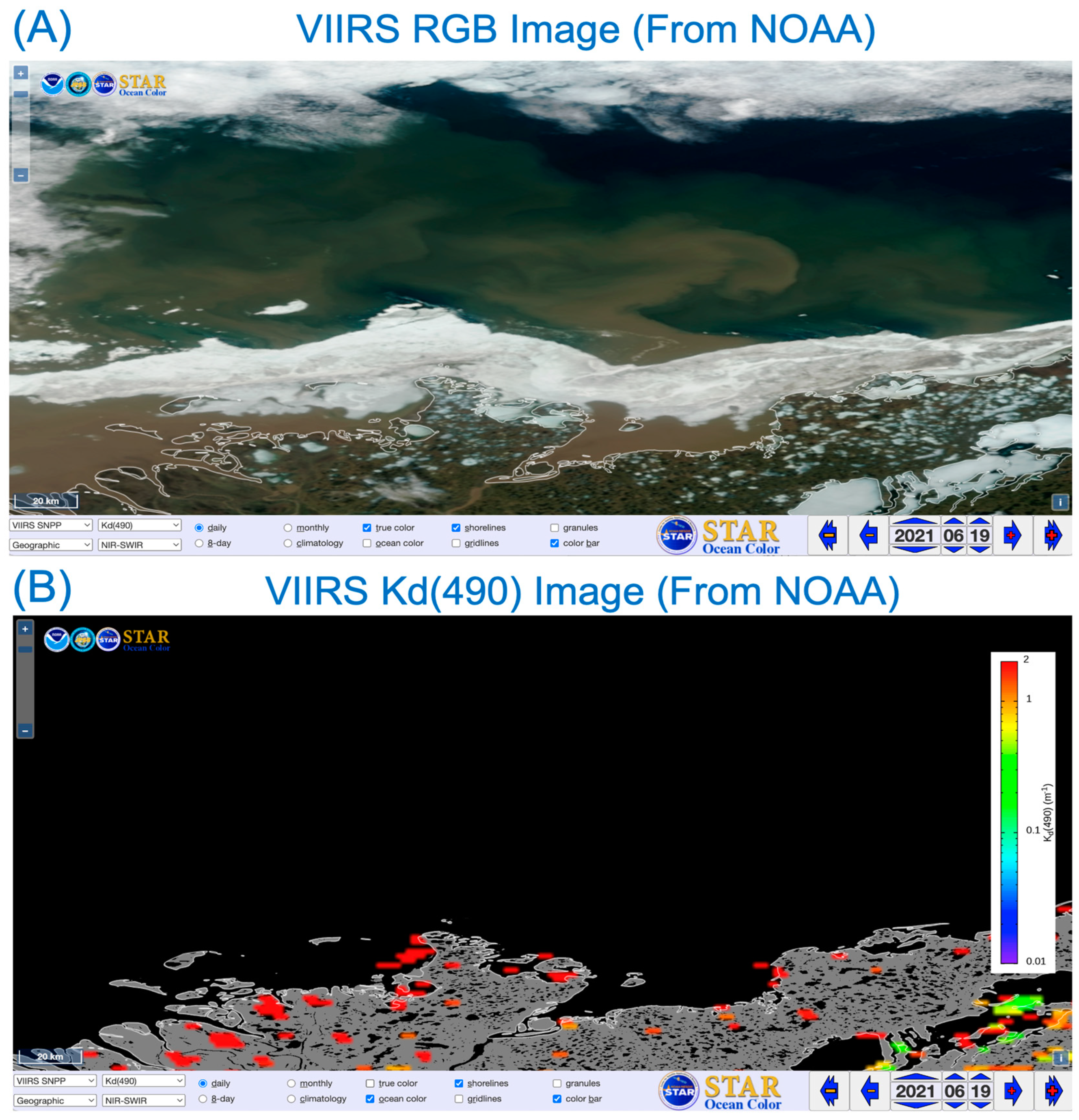
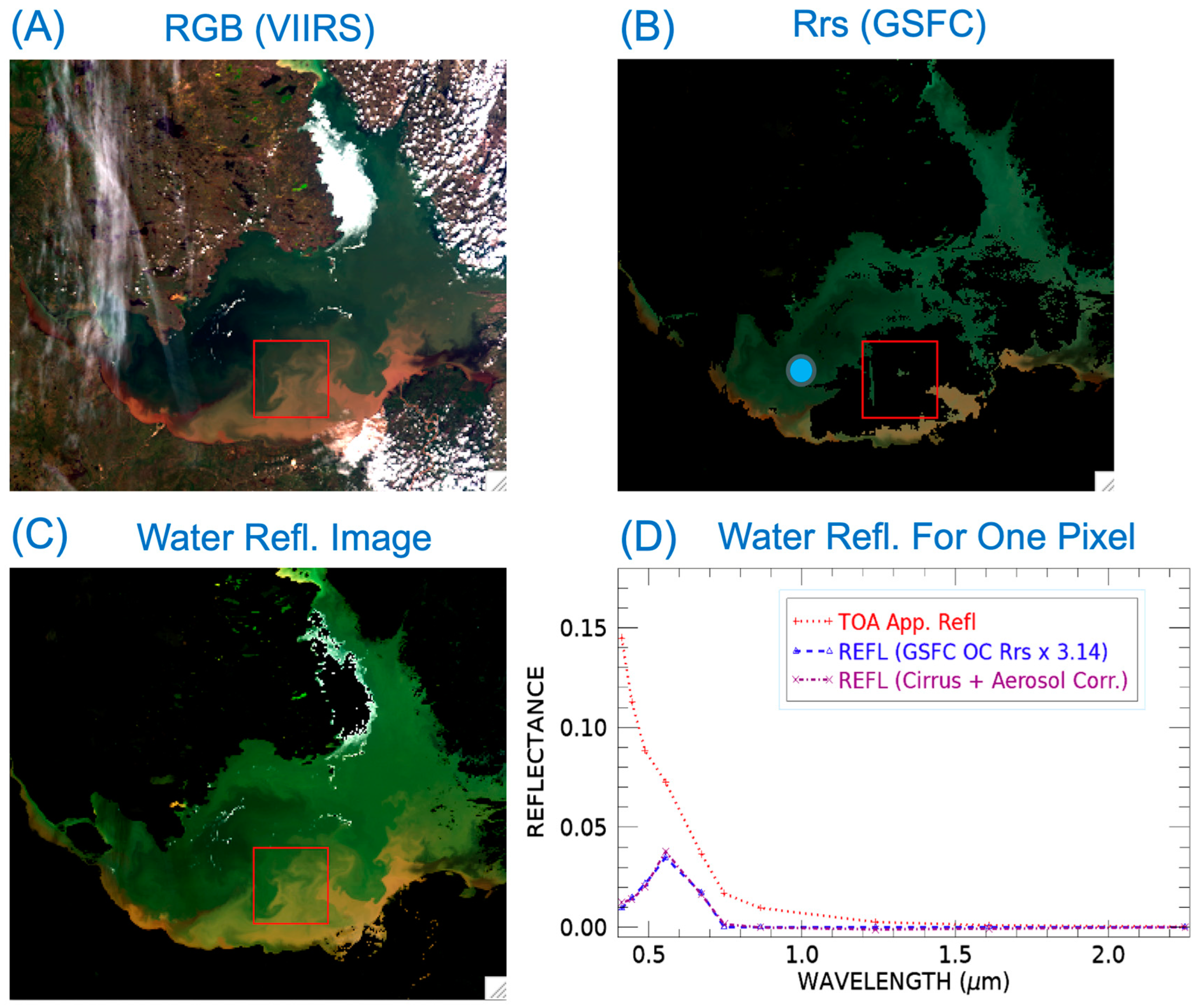
3.2. A VIIRS Scene over Turbid Arctic Lake, 19 June 2021

Figure 8 shows the second case of water-leaving reflectance retrievals from a VIIRS data set acquired over turbid Arctic waters on 19 June 2021. Figure 8A is a portion of the VIIRS RGB image located at an approximate latitude of 61.5° N and 115.5° W (Great Slave Lake in Canada). Clouds, land, and brownish-colored turbid waters are seen. Figure 8B is the RGB image processed from the NASA-released L2 Rrs ocean color data set. Over large portions of turbid water areas, in particular, the area outlined in the square, Rrs values are not derived with the NASA algorithm. Figure 8C is the water-leaving reflectance image retrieved with ATREMsimplify. Spatially contiguous turbid water features are retrieved. Figure 8D shows a comparison of reflectance retrievals over a pixel located at the center of the large blue dot (marked in Figure 8B), where both the NASA algorithm and our algorithm made retrievals. The retrieved results in the visible spectral region with the NASA Rrs algorithm (see the blue-colored line) and our algorithm (the purple-colored line) agree quite well. The lack of spatial coverage over turbid waters, as shown in Figure 8B, can be attributed to the strict masking criteria implemented in the NASA Rrs algorithm. It should be pointed out that, in the upper right portion of Figure 8C, some pixels near cloud edges were misclassified as water pixels. A refined cloud masking scheme needs to be developed in the future.

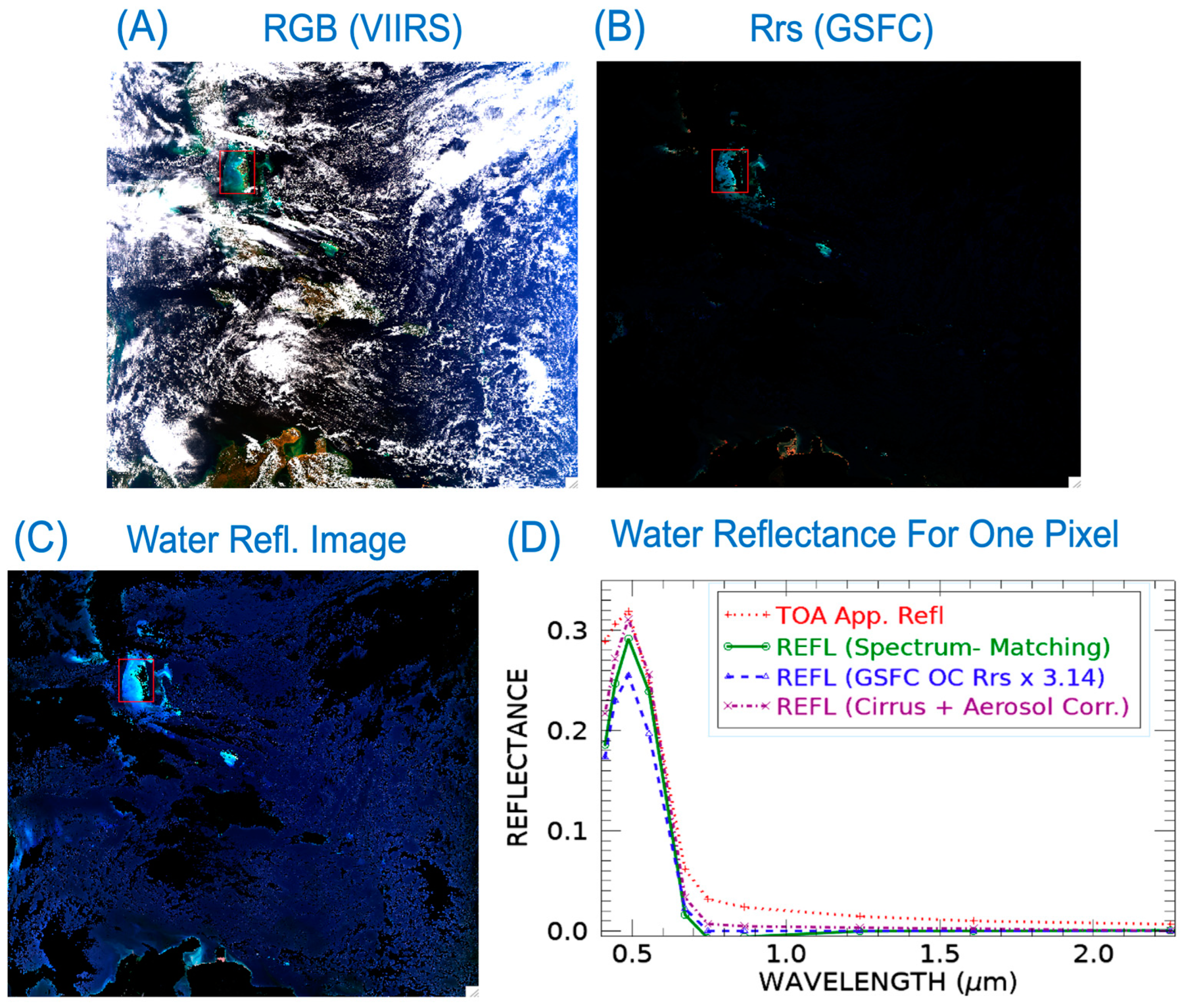
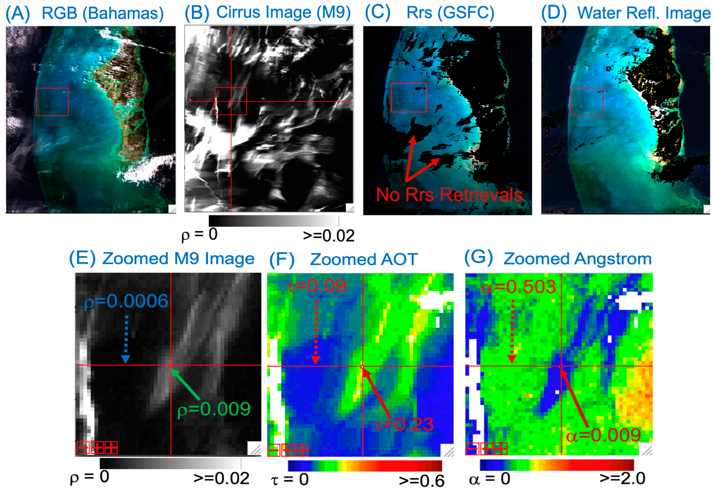
3.3. A VIIRS Scene Covering Bahamas Banks Area, 11 January 2015

Figure 9 shows the third case of water-leaving reflectance retrievals from a VIIRS data set acquired over Bahamas Banks on 11 January 2015. The waters in Bahamas banks are generally clear and can be classified as Case 1 waters. However, Bahamas Banks is optically complex, or Case 2, because solar light can reach the sea floor, reflect, and scatter by bright sand and dense seagrass, which contributes significantly to water-leaving reflectances. Figure 9A is the RGB image of the full VIIRS scene. The bright Bahamas Banks area is in the upper left portion of the scene. Figure 9B is the Rrs image processed from the NASA-released L2 data set. Figure 9C is the water-leaving reflectance image retrieved with ATREMsimplify. By comparing Figure 9C with Figure 9B, it is seen that our retrievals have more processed pixels than the NASA retrievals, particularly over the lower half of the scene and near the left edge of the scene. Figure 9D shows comparisons of water-leaving reflectances retrieved with the NASA Rrs algorithm (blue line), ATREMmatch (green line), and ATREMsimplify (purple line) for a bright pixel having a strong reflection from the sandy seafloor. The water-leaving reflectances in the visible agree reasonably well with the three retrieving algorithms, but the values from the NASA Rrs algorithm are on the lower end.
Figure 10 shows images covering only the portion around the Bahamas Banks area. Figure 10A is the RGB image, Figure 10B is the M9 band cirrus image, Figure 10C is the RGB of the Rrs image processed from the NASA-released L2 data product, and Figure 10D is an RGB of the water reflectance image retrieved with ATREMsimplify. By comparing Figure 10C with Figure 10B, it is seen that the NASA algorithm masks out areas covered by thicker cirrus clouds, and no Rrs retrievals are made. Our combined cirrus and aerosol removal algorithm (ATREMsimplify) is able to retrieve water-leaving reflectances over cirrus-affected pixels and results in a more spatially uniform water-leaving reflectance image (see Figure 10D).
There is a common small square area outlined by red-colored line segments in Figure 10A–D images. The zoomed-in cirrus image is shown in Figure 10E, where two very thin cirrus features extending from the upper right to the lower left are seen. Figure 10F shows the corresponding zoomed-in AOT image processed from the NASA L2 data product. Figure 10G is the corresponding Angstrom image. By comparing Figure 10E cirrus image with Figure 10F,G images, it is obvious that the thin cirrus spatial patterns in Figure 10E are reproduced exactly in Figure 10F AOT image and Figure 10G Angstrom image. At the center pixel of the Figure 10E image, the M9 cirrus band reflectance value is 0.009, indicating that the cirrus is very thin (<0.02). The AOT value for the same pixel in Figure 10F is 0.23, and the Angstrom value in Figure 10G is 0.009. Slight to the left of the center cirrus pixel in Figure 10E is a clear pixel with the M9 band reflectance value of 0.0006 (close to zero, but above the 0.00016 noise level of the M9 band (see Figure 5)). The corresponding AOT value for the same pixel in Figure 10F image is 0.09 (close to the climatological AOT value of about 0.1), and the Angstrom value for the same pixel in Figure 10G image is 0.503. The cirrus spatial patterns in Figure 10E–G images and the values placed inside these images demonstrate that the NASA Rrs algorithm treats thin cirrus clouds as ‘white’ aerosols during the atmospheric correction process. The AOT values are over-estimated, and the Angstrom values are under-estimated for pixels contaminated by thin cirrus clouds. Therefore, the AOT and Angstrom data products derived with the NASA Rrs algorithm are not ideally suited to serve as the long-term climate data records (CDRs).

3.4. A VIIRS Scene over the East China Sea, 6 April 2012

Figure 11 shows the fourth case of water-leaving reflectance retrievals from a VIIRS data set acquired over the east coast of China on 6 April 2012. Waters in this area are often quite turbid due to outflows from the Yangtze and other rivers, and the satellite Rrs data products are frequently not retrieved. Figure 11A is the VIIRS RGB image where clouds, land, and colored water features are seen. Figure 11B is the M9 band cirrus image. Figure 11C is the Rrs image processed from the NASA-released L2 ocean color data set. Figure 11D is the TOA reflectance image for the VIIRS 0.865 μm band (M7) image. By comparing the Figure 11C image with the Figure 11A image, it is seen that the NASA Rrs algorithm produces retrieval results only over the small upper portion of the scene since everything else is masked out. Over the middle and bottom portions of turbid waters, Rrs retrievals are hardly made. Figure 11D shows that TOA reflectance values for the 0.865 μm atmospheric correction band used by the NASA Rrs algorithm over the very turbid water areas (see middle and bottom portions of Figure 11A image) are 0.05 or larger. The bright water pixels are automatically masked out by the NASA Rrs algorithm, and they result in no Rrs retrievals. Figure 11E is the water-leaving reflectance image retrieved with ATREMsimplify. We are able to make retrievals over not only bight ocean waters but also inland lake waters in the left portion of Figure 11E. We are also able to recover water features over thin cirrus-affected pixels (with M9 band TOA reflectance values smaller than 0.08). By comparing the Figure 11C image with the Figure 11E image, it is seen that the spatial area over which we have retrievals is significantly larger than the area where the NASA algorithm made retrievals. Figure 11F shows an example of water-leaving reflectance derivations over one pixel where the NASA algorithm and our algorithms (ATREMmatch and ATREMsimplify) have successful retrievals. All the algorithms are able to obtain the reflectance peak near 0.55 μm. Again, the visible band water reflectance values obtained with the NASA Rrs algorithm are smaller than those retrieved with our algorithms.

4. Discussion

The present NASA atmospheric correction algorithms used for operational generation of the L2 ocean color data products, including remote sensing reflectances, aerosol optical thicknesses, and Angstrom coefficients from MODIS, VIIRS, and PACE OCI data have heritages traceable to the GW94 algorithm, while the GW94 algorithm was originally designed for atmospheric correction over Case 1 waters. Due to this, these algorithms often have built-in masks that effectively screen out turbid water pixels. The extension of these algorithms for retrieving water-leaving reflectances over Case 2 waters often results in no retrievals. In this article, we propose relaxing the strict masking criteria so that bright Case 2 water pixels are not automatically masked out in the presence of thin cirrus cloud and sun glint contamination, and retrievals can be made with our VIIRS versions of water-leaving reflectance algorithms, i.e., ATREMmatch, and ATREMsimplify. When the effects of thin cirrus clouds and sun glint are weak, the selection of the M11 band TOA reflectance values smaller than 0.03 for water pixel identifications is a proper choice [31]. However, it is necessary to increase the M11 band’s threshold value to about 0.12 in order not to screen out bright Case 2 waters in the presence of cirrus cloud and sun glint effects for VIIRS data sets acquired over Black Sea, Caspian Sea, Bahamas Banks, and East China Sea. In the future, the M11 band threshold values for water/land pixel separations over different geographic regions can be set differently for improved masking purposes.
In our algorithms, we masked out pixels with the M9 band TOA reflectance values greater than or equal to 0.08 as cloudy pixels. Through visual inspections of many visible band images contaminated by cirrus clouds with M9 band TOA reflectance values less than about 0.08, we observed that the spatial features of bright Case 2 waters could be seen in the relevant visible band images [23]. Therefore, we made cirrus removals first, followed by aerosol corrections for such cirrus-contaminated water pixels.

5. Summary and Conclusions

We have developed two effective algorithms combining cirrus correction and aerosol corrections for improved retrieval of water-leaving reflectances over Case 2 waters from VIIRS data. One version is to (1) remove cirrus cloud effects, (2) derive aerosol model and optical thickness on a pixel-by-pixel basis using a spectrum-matching method, and (3) obtain water-leaving reflectances of Case 2 waters according to Equation (3). This version of the algorithm is referred to as ATREMmatch. The other version is to 1) remove cirrus cloud effects, (2) assume a climatological aerosol model and optical depth and approximately derive the water-leaving reflectances on a pixel-by-pixel basis, and (3) subtract out the M11 band reflectance value obtained in Step 2 for all VIIRS bands on a pixel-by-pixel basis to remove sun glint and residual ‘white’ aerosol effects to obtain improved estimates of water-leaving reflectances. This version is referred to as ATREMsimplify. Retrievals with both algorithms have been made over about 50 selected VIIRS scenes acquired over different geographic regions and in different years. The retrieved results with both algorithms agree quite well, but the speed of code execution with ATREMsimplify is approximately 20 times faster than that with ATREMmatch. Our retrieved results shown in Figure 7, Figure 8, Figure 10 and Figure 11 demonstrate that we are able to retrieve water-leaving reflectances over very turbid waters (both ocean and large inland lakes) and with cirrus contaminations. Spatially contiguous water-leaving reflectance images are obtained. In these figures, the retrieval results from the NASA Rrs algorithm are also shown; most bright Case 2 water pixels, as well as those pixels affected by cirrus clouds, are masked out by the algorithm, and no retrievals are made (see Figure 11C). We would like to suggest that the strict land and cloud masking criteria implemented in the NASA Rrs algorithm should be relaxed in order to make the algorithm effective for retrievals over Case 2 waters. We have demonstrated without doubt that the NASA Rrs algorithm’s treatment of thin cirrus clouds as aerosols during atmospheric correction processes results in overestimated aerosol optical thicknesses and underestimated aerosol Angstrom coefficient (see Figure 10E–G). Therefore, the AOT and Angstrom data products retrieved with the NASA Rrs algorithm from VIIRS data are not sufficiently reliable to serve as long-term climate data records. We have also demonstrated that in Case 2, waters in the absence of cirrus contamination the water-leaving reflectances for the VIIRS M6 (0.75 μm) band are not close to zero (see Figure 7A,F,G, Figure 9D and Figure 11F), and the NASA Rrs algorithm can slightly overestimate aerosol Angstrom coefficient, which result in slight overestimates of atmospheric scattering effects in visible bands and underestimates of water-leaving reflectances of visible bands. Overall, there is still room for improvements to the NASA Rrs algorithm in order to make the algorithm suitable for global retrieval of water-leaving reflectances over Case 2 waters.

Author Contributions

B.-C.G. originated the idea of combining cirrus correction and aerosol correction for improved retrieval of water-leaving reflectances over Case 2 waters. R.-R.L. developed modules for automating the atmospheric correction process and contributed to data analysis. M.J.M. and S.C.M. contributed to the data analysis and in helping to obtain the research funding for an NRL internal 6.2 research project. All authors have read and agreed to the published version of the manuscript.

Funding

This research was funded by the Office of Naval Research under the NRL 6.2 Base Funding program. The funding element was 62435N.

Institutional Review Board Statement

Approved for public release. Distribution is unlimited.

Data Availability Statement

All data are available upon request.

Acknowledgments

The authors are grateful to Pengwang Zhai at the Physics Department, University of Maryland at Baltimore County, for extensive calculations of lookup tables with his vector version of the radiative transfer code and for comments to improve the manuscript, and to Menghua Wang with the Satellite Oceanography and Climatology Division of NOAA for pointing out the availability of a NOAA public web site (OCView) to view VIIRS RGB images and NOAA-retrieved ocean color product images.

Conflicts of Interest

The authors declare no conflicts of interest.

References

  1. Groom, S.; Sathyendranath, S.; Ban, Y.; Bernard, S.; Brewin, R.; Brotas, V.; Brockmann, C.; Chauhan, P.; Choi, J.K.; Chuprin, A.; et al. Satellite ocean colour: Current status and future perspective. Front. Mar. Sci. 2019, 6, 485. [Google Scholar] [CrossRef] [PubMed]
  2. McClain, C.R.; Franz, B.A.; Werdell, P.J. Genesis and evolution of NASA’s satellite ocean color program. Front. Remote Sens. 2022, 3, 938006. [Google Scholar] [CrossRef]
  3. Bisson, K.M.; Boss, E.; Werdell, P.J.; Ibrahim, A.; Frouin, R.; Behrenfeld, M.J. Seasonal bias in global ocean color observations. Appl. Opt. 2021, 60, 6978–6988. [Google Scholar] [CrossRef] [PubMed]
  4. Meister, G.; Franz, B.A.; McClain, C.R. Influence of thin cirrus clouds on ocean color products. Proc. SPIE 2009, 7459, 745903-1–745903-12. [Google Scholar]
  5. Bailey, S.W.; Franz, B.A.; Werdell, P.J. Estimation of near-infrared water leaving reflectance for satellite ocean color data processing. Opt. Express 2020, 18, 7521–7527. [Google Scholar] [CrossRef]
  6. Available online: https://www.star.nesdis.noaa.gov/socd/mecb/color/ocview/ocview.html (accessed on 1 November 2024).
  7. Wang, M.; Son, S.; Harding, L.W. Retrieval of diffuse attenuation coefficient in the Chesapeake Bay and turbid ocean regions for satellite ocean color applications. J. Geophys. Res. 2009, 114, C10011. [Google Scholar] [CrossRef]
  8. Ibrahim, A.; Franz, B.; Bailey, S.; Werdell, J.; Ahmad, Z.; Mobley, C. Remote Sensing Reflectance. Available online: https://www.earthdata.nasa.gov/apt/documents/rrs/v1.1 (accessed on 3 December 2024).
  9. Franz, B.A.; Werdell, P.J.; Meister, G.; Kwiatkowska, E.J.; Bailey, S.W.; Ahmad, Z.; McClain, C.R. MODIS land bands for ocean remote sensing applications. In Proceedings of the Ocean Optics XVIII, Montreal, QC, Canada, 9–13 October 2006. [Google Scholar]
  10. Gao, B.C.; Li, R.R. Removal of thin cirrus scattering effects in Landsat 8 OLI images using the cirrus detecting channels. Remote Sens. 2017, 9, 834. [Google Scholar] [CrossRef]
  11. Gao, B.C.; Li, R.R. The VIIRS cirrus reflectance algorithm. Sensors 2023, 23, 2234. [Google Scholar] [CrossRef]
  12. Gao, B.C.; Li, R.R. A multi-band atmospheric correction algorithm for deriving water leaving reflectances over turbid waters from VIIRS data. Remote Sens. 2023, 15, 425. [Google Scholar] [CrossRef]
  13. Moyer, A.; McIntire, J.; Young, J.; McCarthy, J.K.; Waluschka, E.; Xiong, X.; De Luccia, F.J. JPSS-1 VIIRS prelaunch polarization testing and performance. IEEE Trans. Geosc. Remote Sens. 2017, 55, 2463–2476. [Google Scholar] [CrossRef]
  14. Gao, B.-C.; Montes, M.J.; Ahmad, Z.; Davis, C.O. Atmospheric correction algorithm for hyperspectral remote sensing of ocean color from space. Appl. Opt. 2000, 39, 887–896. [Google Scholar] [CrossRef] [PubMed]
  15. Wilson, T.; Davis, C. Naval EarthMap Observer (NEMO) Satellite. 1999. Available online: https://www.spiedigitallibrary.org/conference-proceedings-of-spie/3753/0000/Naval-EarthMap-Observer-NEMO-satellite/10.1117/12.366268.pdf (accessed on 19 November 2024).
  16. Vane, G.; Green, R.O.; Chrien, T.G.; Enmark, H.; Hansen, E.G.; Porter, W.M. The Airborne Visible/Infrared Imaging Spectrometer. Remote Sens. Environ. 1993, 44, 127–143. [Google Scholar] [CrossRef]
  17. Gordon, H.; Wang, M. Retrieval of water-leaving radiance and aerosol optical thickness over the oceans with SeaWiFS: A preliminary algorithm. Appl. Opt. 1994, 33, 443–452. [Google Scholar] [CrossRef]
  18. Fraser, R.S.; Mattoo, S.; Yeh, E.-N.; McClain, C.R. Algorithm for atmospheric and glint corrections of satellite measurements of ocean pigment. J. Geophys. Res. 1997, 102, 17107–17118. [Google Scholar] [CrossRef]
  19. Fraser, R.; Ferrare, R.; Kaufman, Y.J.; Mattoo, S. Algorithm for atmospheric corrections of aircraft and satellite imagery. NASA Tech. Memo. 1989, 13, 100751. [Google Scholar] [CrossRef]
  20. Tanre, D.; Deroo, C.; Duhaut, P.; Herman, M.; Morcrette, J.J.; Perbos, J.; Deschamps, P.Y. Description of a computer code to simulate the satellite signal in the solar spectrum: The 5S code. Int. J. Remote Sens. 1990, 11, 659–668. [Google Scholar] [CrossRef]
  21. Ahmad, Z.; Fraser, R.S. An iterative radiative transfer code for ocean-atmosphere systems. J. Atmos. Sci. 1982, 39, 656–665. [Google Scholar] [CrossRef]
  22. Gao, B.-C.; Montes, M.J.; Li, R.-R.; Dierssen, H.M.; Davis, C.O. An atmospheric correction algorithm for remote sensing of bright coastal waters using MODIS land and ocean channels in the solar spectral region. IEEE Trans. Geosc. Remote Sens. 2007, 45, 1835–1843. [Google Scholar] [CrossRef]
  23. Available online: https://modis.gsfc.nasa.gov/sci_team/meetings/201505/presentations/atmosphere/gao.pdf (accessed on 19 November 2024).
  24. Zhai, P.W.; Hu, Y.X. An improved pseudo spherical shell algorithm for vector radiative transfer. J. Quant. Spectrosc. Radiat. Transf. 2022, 282, 108132. [Google Scholar] [CrossRef]
  25. Zhai, P.W.; Gao, M.; Franz, B.A.; Werdell, P.J.; Ibrahim, A.; Hu, Y.; Chowdhary, J. A radiative transfer simulator for PACE: Theory and applications. Front. Remote Sens. 2022, 3, 840188. [Google Scholar] [CrossRef]
  26. Nazaryan, H.; McCormick, M.P.; Menzel, W.P. Global characterization of cirrus clouds using CALIPSO data. J. Geophys. Res. 2008, 113, D16211. [Google Scholar] [CrossRef]
  27. Gao, B.C.; Kaufman, Y.J.; Tanre, D.; Li, R.R. Distinguishing tropospheric aerosols from thin cirrus clouds for improved aerosol retrievals using the ratio of 1.38-mm and 1.24-mm channels. Geophys. Res. Lett. 2002, 29, 1890. [Google Scholar] [CrossRef]
  28. Moran, M.S.; Jackson, R.D.; Slater, P.N.; Teillet, P.M. Evaluation of simplified procedures for retrieval of land surface reflectance factors from satellite sensor output. Remote Sens. Environ. 1992, 41, 169–184. [Google Scholar] [CrossRef]
  29. Fraser, R.S.; Kaufman, Y.J. The relative importance of aerosol scattering and absorption in remote sensing. IEEE Transc. Geosci. Remote Sens. 1985, GE-23, 625–633. [Google Scholar] [CrossRef]
  30. Mobley, C.D.; Werdell, J.; Franz, B.; Ahmad, Z.; Bailey, S. Atmospheric Correction for Satellite Ocean Color Radiometry; NASA T/M-2016-217551; NASA Goddard Space Flight Center: Greenbelt, MD, USA, 2016; p. 73.
  31. Hedley, J.; Harborne, A.; Mumby, O. Simple and robust removal of sun glint for mapping shallow-water benthos. Int. J. Remote Sens. 2005, 26, 2107–2112. [Google Scholar] [CrossRef]
Figure 1. A VIIRS RGB image (A) and the corresponding Kd(490) image (B) obtained from NOAA. The VIIRS data were acquired on 19 June 2021 over Arctic regions.
Oceans 06 00028 g001
Figure 2. Bandpasses of VIIRS M bands in the 0.4–2.5 μm solar spectral range. A measured reflectance spectrum over a shallow water area having reflection from the sea floor and a typical TOA cirrus reflectance spectrum acquired with the AVIRIS-NG spectrometer onboard an ER-2 aircraft at an altitude of 20 km are also shown.
Oceans 06 00028 g002
Figure 3. Illustration of solar ray paths for a band centered near 1.38 μm and an atmospheric window band in a simplified atmosphere–surface system.
Oceans 06 00028 g003
Figure 4. (A)—portion of a VIIRS RGB image acquired over Baltic Sea on 11 July 2014 during plankton blooming event, (B)—the corresponding M9 band image, and (C)—cirrus-removed RGB image.
Oceans 06 00028 g004
Figure 5. An illustration of noise estimates from a VIIRS image for M1–M11 bands.
Oceans 06 00028 g005
Figure 6. (A)—a color image processed from a set of MODIS data acquired over the coastal area in northeastern part of Australia in August of 2002 (Red: 0.645 μm; Green: 0.55 μm; Blue: 0.47 μm), (B)—the color image processed from the water-leaving reflectances (for the same three bands) retrieved with our spectrum-matching version of ATREM algorithm for MODIS data processing, (C)—the derived AOT image, and (D)—examples of water-leaving reflectances retrieved with our algorithm and with the NASA MODIS Rrs algorithm over a deep ocean area and a turbid water area.
Oceans 06 00028 g006
Figure 7. (A)—an RGB image processed from a set of VIIRS data acquired over a chlorophyll bloom off the east coast of Argentina on 17 December 2018, (B)—the corresponding VIIRS M9 band cirrus image, (C)—the Rrs RGB image processed from NASA released L2 data product, (D)—the AOT image also processed from the NASA data product, (E)—water leaving RGB reflectance image retrieved with our algorithm (ATREMsimplify) that combined cirrus and aerosol corrections, (F)—various reflectances for one water pixel, (G)—TOA image for the VIIRS 0.75 μm band (M6) where the spatial patterns of chlorophyll blooming were present and the water-leaving reflectances were not zero, and (H)—TOA image for the 0.865 μm band, where the chlorophyll spatial features were nearly absent.
Oceans 06 00028 g007
Figure 8. (A)—an RGB image processed from a VIIRS data set acquired over turbid Arctic lake waters on 19 June 2021, (B)—and RGB Rrs image processed from NASA released L2 data product, (C)—an RGB water-leaving reflectance images retrieved with our algorithm (ATREMsimplify) that combined cirrus and aerosol corrections, and (D)—comparisons between water-leaving reflectances over a pixel where both the NASA algorithm and our algorithm made retrievals.
Oceans 06 00028 g008
Figure 9. (A)—an RGB image processed from a VIIRS data set covering Bahamas Banks area on 11 January 2015, (B)—an RGB of the Rrs image processed from NASA released L2 data product, (C)—an RGB of the water-leaving reflectance image retrieved with our algorithm (ATREMsimplify) that combined cirrus and aerosol corrections, and (D)—comparisons between water-leaving reflectances over a bright sandy pixel retrieved with the NASA Rrs algorithm, ATREMmatch, and ATREMsimplify.
Oceans 06 00028 g009
Figure 10. (A)—the VIIRS RGB image covering Bahamas Banks area, (B)—the corresponding M9 band cirrus image, (C)—the Rrs image processed from NASA released L2 data product, (D)—the water reflectance image retrieved with ATREMsimplify, (E)—the zoomed-in M9 band cirrus image, (F)—the zoomed-in AOT image processed to form the NASA L2 Rrs data product, and (G)—the zoomed-in Angstrom image obtained from the NASA L2 Rrs product.
Oceans 06 00028 g010
Figure 11. (A)—the VIIRS RGB image for a scene acquired over the east coast of China on April 6, 2012, (B)—the M9 band cirrus image, (C)—and RGB from the Rrs image processed from NASA released L2 data set, (D)—the TOA reflectance image for the VIIRS atmospheric correction band (M7) centered near 0.865 μm, (E)—an RGB from the water-leaving reflectance image retrieved with ATREMsimplify, and (F)—comparisons between water-leaving reflectances over a turbid water pixel retrieved with the NASA Rrs algorithm, ATREMmatch, and ATREMsimplify.
Oceans 06 00028 g011
Table 1. The names, widths, and nadir spatial resolution (m) of some VIIRS bands.
BandsWavelength (μm)Resolution (m)
M10.405–0.425750
M20.435–0.455750
M30.480–0.500750
M40.545–0.565750
M50.663–0.684750
M60.736–0.756750
M70.846–0.885750
M81.230–1.250750
M9 (Cirrus Band)1.368–1.388750
M101.580–1.640750
M112.225–2.275750
Disclaimer/Publisher’s Note: The statements, opinions and data contained in all publications are solely those of the individual author(s) and contributor(s) and not of MDPI and/or the editor(s). MDPI and/or the editor(s) disclaim responsibility for any injury to people or property resulting from any ideas, methods, instructions or products referred to in the content.

