3D Structure of the Ras Al Hadd Oceanic Dipole

Abstract

In the Arabian Sea, southeast of the Arabian peninsula, an oceanic dipole, named the Ras Al Hadd (RAH) dipole, is formed each year, lying near the Ras Al Hadd cape. The RAH dipole is the association of a cyclonic eddy (CE) to the northeast, with an anticyclonic eddy (AE) to the southwest. This dipole intensifies in the summer monsoon and disappears during the winter monsoon. This dipole has been described previously, but mostly for its surface expression, and for short time intervals. Here, we describe the 3D structure of this dipole over the 2000–2015 period, by combining colocalized ARGO float profiler data (a total of 7552 profiles inside and outside the RAH dipole) with angular momentum eddy detection and tracking algorithm (AMEDA) surface data. We show first the different water masses in and near the RAH dipole. The presence of the Persian Gulf water (PGW) below 200 m depth is confirmed in both eddies. Arabian Sea high salinity water (ASHSW) is found exclusively in the AE; a layer of fresh and cold water is observed above 100 m depth in both eddies. By analyzing the potential density structures, we show that the CE has a surface-intensified structure while the AE is subsurface-intensified. The sea level anomaly shows a 0.04 m elevation above the AE and a 0.2 m depression over the CE. The CE has a faster geostrophic velocity, (vertical velocity, respectively) 0.6 m s⁻¹ than the AE, 0.15 m s⁻¹ (respectively, 3 m day⁻¹ for the CE and 0.6 m day⁻¹ for the AE). After presenting the vertical structure of the dipole, we show the dominance of the nonlinear Ekman pumping in the CE over the linear pumping affecting the dipole. As a consequence, we explain the CE’s longer lifetime by its intensity and shallowness, and by its sensitivity to the interaction with the atmosphere (in particular the wind stress) and with neighboring eddies. We examined the possible (co)existence of symmetric, barotropic, and baroclinic instabilities in both eddies. These instabilities coexist near the surface in both eddies. They are intensified for the CE, which suggests that the CE is unstable and the AE is rather stable or may need a long time to be unstable.

1. Introduction

In the past few decades, interest in the Arabian Sea currents and hydrology has increased due to geopolitical reasons. This area includes a very peculiar western boundary current due to the variation in land and ocean masses in the Indian Ocean. In the northern Indian Ocean lies the Arabian Sea, which borders Asia and Africa (Figure 1). The Arabian monsoon affects the dynamics of the regional ocean [1].

Indeed, the Arabian Sea and its marginal gulfs are affected by the seasonal monsoon atmospheric regimes and by the North Equatorial current [1,2].

Monsoons have their own variability: southwesterly winds blow from May to October, while northeasterly winds blow from December to February. Inter-monsoon periods (spring and fall) are characterized by weak winds that blow randomly. Furthermore, the atmospheric circulation is influenced by the orography (high mountains), which strengthens the winds over the Arabian Sea.

Figure 1. (a) Bathymetry of the Arabian Sea and its marginal gulfs from the ETOPO2 database [3]. (b) Snapshot of the Ras al Hadd dipole in summer 2020 with the cyclone to the northeast and the anticyclone to the southwest (from the Ocean Virtual laboratory web portal (ESA, OceanDataLab, accessed on 1 December 2020) [4].

Figure 1. (a) Bathymetry of the Arabian Sea and its marginal gulfs from the ETOPO2 database [3]. (b) Snapshot of the Ras al Hadd dipole in summer 2020 with the cyclone to the northeast and the anticyclone to the southwest (from the Ocean Virtual laboratory web portal (ESA, OceanDataLab, accessed on 1 December 2020) [4].

These mountains favor intense winds in the Gulf of Aden and the southern Red Sea during the winter, and along the Somalian coast and the northern Arabian Sea during the summer [5].

Coastal currents, such as the Omani Coastal Current (OCC) and the West India Coastal Current (WICC), are also affected by monsoon winds. The OCC flows northeastward during the summer and southeastward in the winter; the WICC circulates southward during the summer and northward during the winter [6].

Wind orientation and intensity cause upwelling and downwelling events, resulting in vertical mixing of surface waters in these ocean currents [4]. During the summer, The upwelled waters, mainly the PGW and RSW, are advected through these currents along the Indian and Omani coasts, respectively [7,8,9]. The PGW and RSW, salty and warm water masses, originate from the Persian Gulf and the Red Sea. These semi-enclosed areas are subject to high evaporation rates and heat fluxes [8,10]. The PGW, mainly observed in the Gulf of Oman, has a signature between 100 and 600 m in depth [11]. Its horizontal signature in temperature and salinity decreases exponentially from the Strait of Hormuz to the offshore [12]. The RSW is present mainly in the Gulf of Aden and along the west side of the Arabian Sea. It retains a significant signature in the northern and eastern parts of the Arabian Sea, while it is more diluted to the southwest [8,12]. The study area tends to react quickly to changes in the mesoscale patterns of E-P (freshwater fluxes), which alters the characteristics of the water formed in both PGW and RSW.

PGW and RSW exhibit complex biogeochemical responses through mesoscale eddies. These eddies propagate and diffuse these outflows. In the Arabian Sea, mesoscale eddies range in size from about 100 to 200 km. Based on theory, the most intense mesoscale eddies ($\mathcal{O}(100$ km)) [3].

These mesoscale eddies are spread in different regions of the Arabian Sea. In the Gulf of Aden, a sequence of large eddies is observed each year [13,14]. The Gulf of Aden eddy is one of these large eddies. It appears during early spring and splits during the summer [13,15]. Splitting occurs as a result of the Ekman divergence and thermocline motion. This gives birth to two anticyclonic eddies: the Summer Eddy (SE) and the Lee Eddy (LE) [13]. In contrast to the LE, the SE intensifies while moving westward in the Gulf of Aden, while the LE remains stationary near Socotra Island [14]. They have radii of about 50 km, and their intensification is related to the Ekman convergence.

Mesoscale eddies can be formed by pairs of cyclones/anticyclones: oceanic dipoles. In the Arabian Sea, these dipoles have been observed in the GO: the Ras Al Hamra and Ras Al Hadd dipoles [4,11].

The dipole of Ras Al Hamra is formed by a couple of deep-reaching eddies, a cyclone to the west and an anticyclone to the east. The PGW is ejected to the northern Arabian Sea via this dipole. Seasonal mesoscale eddies also affect this ejection [11].

The Ras Al Hadd (RAH) dipole, located southwest of the Ras Al Hamra dipole, consists of a CE to the northeast and an AE to the southwest. This dipole appears during the summer monsoon and breaks up in the winter [4]. As paired eddies interact dynamically, an intense jet forms between them. This jet is intensified during the summer monsoon [16].

The RAH dipole is composed of long-living eddies at the entrance of the Gulf of Oman. During their life cycle, they interact with neighboring eddies and outflows. The RAH dipole is composed of long-living eddies at the Ras Al Hadd cape. Previous studies have focused on the RAH dipole life cycle and the associated jet. However, the 3D structure of the two eddies composing it, and their interactions with the PGW and other water masses, remain unclear. In this paper, we study the 3D structure of the RAH dipole via ARGO floats and AMEDA (eddy tracking algorithm) outputs. Then, we analyze the signature of different water masses observed inside the pairing eddies. Finally, we compute the dipole sea surface structure and its interaction with the SW and NE monsoon wind regimes.

The paper will be organized as follows: First, we present the colocalization of data (AMEDA outputs and ARGO floats), the methodology behind the composite eddies, the sea surface signature, and Ekman interactions in Section 2. Then, we analyze the life cycle of the pairing eddies between 2000 and 2015 in Section 3: (i) its 3D hydrodynamical structure, (ii) its geostrophic sea surface signature, and (iii) its induced Ekman linear and nonlinear pumpings. These results will be discussed in Section 4. Finally, the conclusions are drawn in Section 5.

2. Materials and Methods

2.1. ARGO Floats

Data between 2000 and 2015 were collected in the Northern Arabian Sea (NAS) by ARGO floats [17], as shown in Figure 2. The valid ARGO floats pressure, temperature, and salinity were downloaded from the Coriolis database (Coriolis Web Site). We collected a total of 7552 ARGO profiles inside and outside the RAH dipole (AE and CE). The profiles outside eddies were collected in a fixed domain near the Indian Coast. However, the profiles inside the RAH dipole are non-uniformly distributed in the NAS region. Despite their non-uniform distribution, the majority of the profiles were found around the Ras Al Hadd cape. The potential density, depth, conservative temperature, and absolute salinity were obtained from these data using the Gibbs SeaWater toolbox [18]. Then, we interpolated the vertical collected profiles linearly between 0 and 1000 m with a resolution of 2 m. This interpolation retains the dynamics we are interested in without biasing the results with artificial noise. In this paper, we averaged the temperature, salinity, and potential density over numerous profiles inside and outside the RAH dipole to obtain averages and radial profiles.

2.2. Eddy Tracking

The angular momentum eddy detection and tracking algorithm (AMEDA) is used in the Arabian Sea for the studied period [19]. The algorithm uses the time series of the sea surface height obtained via a combination of real-time measurements by satellite altimetry, as explained in Ayouche et al. [4]. The AVISO Absolute Dynamic Topographic and the derived geostrophic velocities interpolated on a ${\frac{1}{8}}^{\circ }$ Mercator grid were used as input for the AMEDA algorithm between 2000 and 2015. The algorithm uses the Okubo–Weiss (OW) to identify regions dominated by vorticity or by strain. The mesoscale eddies (with radii R lying between the Rossby radius of deformation (Rd) and 5 × Rd) are identified in regions dominated by vorticity. Finally, the algorithm applies the LNAM (angular momentum) method to identify eddy centers and their nature (cyclone or anticyclone). The RAH dipole was tracked and identified through this algorithm during the studied period [4]. The colocalization was performed inside the eddies delimited by the radius of the maximum closed contours (averaged ${\mathrm{R}}_{\mathrm{end}}$ ∼ 100 km for the CE and AE).

2.3. Colocalization Methodology

For the colocalization method, we used the AMEDA algorithm and ARGO floats lying inside the CE and AE of the RAH dipole. We defined eddies as circular shapes delimited by their outermost closed contour (as showed in the Figure 3). Inside these eddies, if the Euclidean distance between the eddy center and the ARGO float was smaller than the radius, we flagged this profile as colocalized. Due to ARGO float temporal sampling, we performed the colocalization within ±24 h from the AMEDA eddy detection moment. As mentioned in De Marez et al. [3], too long of a delay between the eddy detection and ARGO profiling could lead to an error of colocalization.

Then, a dimensionless distance was defined as $\mathrm{r} = \frac{\mathrm{dR}}{\mathrm{R}}$; where dR is the distance between eddy centers and ARGO floats (as mentioned previously) and R is the eddy radius. For r = 0, the ARGO profile lies at the center of the eddy, and r = 1 means that the profile is at the edge of the eddy. This approach allowed us to average physical properties (salinity, temperature, and potential density) along a radial section.

2.4. 3D Composite Eddy Computing

The 3D structure of the CE and AE was computed in regards to the normalized radius r ∈ [0, 1]. The structure is given in terms of the temperature, salinity, and potential density averaged along the normalized radii with a bin size of 0.05. We assume that the ocean structure outside the eddies (r > 1) is represented by the average temperature, salinity, and potential density in the fixed domain described previously. These radial averages give us structures of T(r,z), S(r,z), and $\rho (r,z)$, while assuming no dependency on $\theta$, i.e., $\frac{dT}{d\theta } = \frac{dS}{d\theta }$ = $\frac{d\rho }{d\theta } = 0$. The radial distribution of the colocalized profiles is given in

Table 1. Number of profiles collected inside the eddies in regard to different classes of their normalized radii.

Eddies	$0<\mathbf{r}<0.25$	$0.25<\mathbf{r}<0.5$	$0.5<\mathbf{r}<1$
AE	34	102	384
CE	105	198	526

. This distribution shows that near the edges ($0.5<\mathrm{r}<1$), the number of profiles increases drastically and, therefore, the composite structure will be more accurate for these classes.

The composite density field is mirrored for r < 0 and smoothed with a Gaussian filter with a normalized radius of 0.4. The latter retains density variations larger than 40 km (the radius of deformation) since the average radius of both eddies is ∼100 km. Then, we use the thermal wind balance to obtain the angular velocity with the assumption that the eddies are axisymmetric and non-divergent ($u_r = 0$), assuming no motion below 1000 m depth [20].

$$u_{\theta }(r,z) = -\frac{g}{f{\rho }_0}{\int }_{-1000}^z{\partial }_r\rho (r,z)dz$$

(1)

We project this angular velocity on Cartesian coordinates (x,y) to obtain the velocity components u and v. Then we use the wind gradient equation to obtain the pressure anomaly $P^{\prime }(x,y,z)$

$$2J(u,v) + f_0\zeta + \beta u = \frac{1}{{\rho }_0}{\nabla }^2{P}^{\prime }$$

(2)

where $J(u,v) = {\partial }_{x}u{\partial }_{y}v-{\partial }_{x}v{\partial }_{y}u$ is the determinant of the Jacobian matrix, $f_0 = 5.6 \times {10}^{-5} {\mathrm{s}}^{-1}$ is the Coriolis parameter, $\beta = {\partial }_{y}f = 2 \times {10}^{-11} {\mathrm{m}}^{-1} {\mathrm{s}}^{-1}$, $\zeta = {\partial }_{x}v-{\partial }_{y}u$ is the relative vorticity, ${\rho }_0 = 1027 \mathrm{kg} {\mathrm{m}}^{-3}$ and ${\nabla }^2$ is the horizontal Laplacian.

This equation has been solved using an iterative procedure with an initial geostrophic guess. We deduce the sea surface height anomaly ${\eta }_A$ as in [21]:

$${\eta }_A = \frac{P^{\prime }(x,y,z = 0)}{g\rho (x,y,z = 0)}-\frac{{\int }_z^0{\rho }^{\prime }(x,y,z)dz}{\rho (x,y,z = 0)}$$

(3)

where g is the gravity acceleration, ${\rho }^{\prime }(x,y,z) = \rho (x,y,z)-{\rho }_{background}\left(z\right)$ is the density anomaly and ${\rho }_{background}\left(z\right)$ is the averaged potential density outside eddies. The surface geostrophic velocities are then deduced as:

$$u_{gs} = -\frac{g}{f_0}{\partial }_y{\eta }_{A}and{v}_{gs} = \frac{g}{f_0}{\partial }_x{\eta }_A$$

(4)

In order to assess the Ekman dynamics in both eddies, we compute the vertical velocity using the Q-omega equation on a beta plane in the spectral Fourier space [21,22]:

$$-{\kappa }^2{N}^2\widehat{w} + f_0^2{\partial }_z^{2}w = ik\beta \widehat{b} + (ik{\widehat{Q}}_x + il{\widehat{Q}}_y)$$

(5)

where $\kappa = (k,l)$ is the horizontal wavenumber vector, $b = -g\frac{\rho }{{\rho }_0}$ is the buoyancy, and $Q_x$ and $Q_y$ are the x and y components of the Q vector.

Finally, the linear and nonlinear Ekman pumping velocities are computed as in Ni et al. [21]:

$$w_{nonlin} = \frac{1}{{\rho }_0{(\zeta + f)}^2}({\tau }_x{\partial }_y\zeta -{\tau }_y{\partial }_x\zeta )$$

(6)

$$w_{lin} = \frac{1}{{\rho }_0(\zeta + f)}({\partial }_x{\tau }_y-{\partial }_y{\tau }_x)$$

(7)

where ${\tau }_x$ and ${\tau }_y$ are the wind stress components assumed as Gaussian in shape with an amplitude varying between 0 and 0.1 $\mathrm{N} {\mathrm{m}}^{-2}$.

2.5. Possible Instabilities in the RAH Dipole

Here, we focus on the necessary conditions of the generation of symmetric, barotropic, and baroclinic instabilities. The occurrence of symmetric instability is determined using Hoskins’ criterion [23]: EPV < 0, where EPV is the Ertel potential vorticity defined as:

$$EPV = EP{V}_h + EP{V}_z = \frac{g}{{\rho }_0}\frac{d{V}_{\theta }}{dz}\frac{d\rho }{dr}-\frac{g}{{\rho }_0}(f_0 + \frac{1}{r}\frac{dr{V}_{\theta }}{dr})\frac{d\rho }{dz}$$

(8)

where $EP{V}_h$ and $EP{V}_z$ are the horizontal and vertical EPV components, g is the gravity acceleration, ${\rho }_0$ is a mean density, $f_0 = 5.6 \times {10}^{-5} {\mathrm{s}}^{-1}$ is the averaged Coriolis parameter around the Ras Al Hadd cape.

Symmetric instabilities can be of different types:

• Gravitational (or static) instability when the stratification is unstable (negative Brunt–Vaisala $N^2 = -\frac{g}{{\rho }_0}\frac{d\rho }{dz}$).
• Inertial instability when the absolute vorticity ($f_0$ + ${\zeta }_z$) is negative.
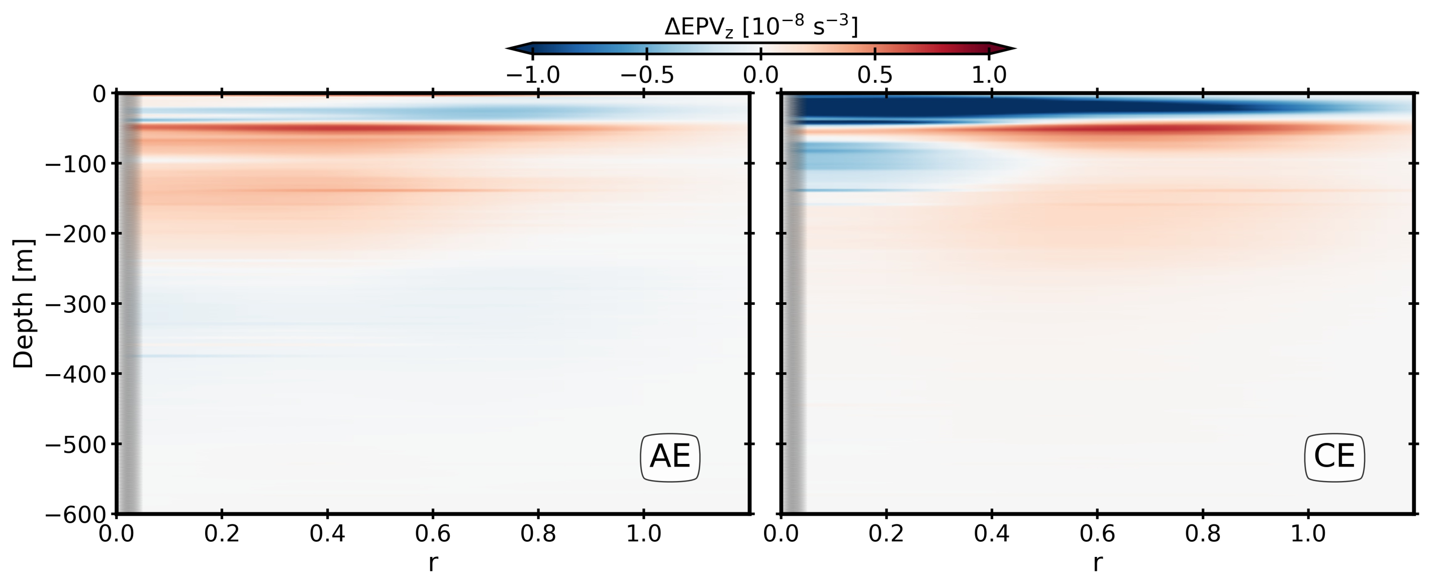
• Pure symmetric when the vertical component of the EPV negatively dominates the EPV, due to a large vertical velocity shear.

On the other hand, the occurrences of barotropic and baroclinic instabilities are determined using the Charney–Stern criteria [24,25,26]: when the horizontal and vertical anomalies of the EPV ($\mathsf{\Delta }EPV(r,z) = EPV(r,z) - EP{V}_{ref}\left(z\right)$ where $EP{V}_{ref}\left(z\right)$ is computed outside the eddies) change signs horizontally and vertically, respectively.

Table 2. Summary of the eventual instabilities related to the eddies.

Instability EPV & Criteria
Symmetric & $EPV = EP{V}_h + EP{V}_z<0$
Barotropic & horizontal sign shifts of $\mathsf{\Delta }EP{V}_z$
Baroclinic & vertical sign shifts of $\mathsf{\Delta }EP{V}_z$

summarizes the criteria of the potential existence of the symmetric, baroclinic, and barotropic instabilities.

3. Results

3.1. Colocalization of the RAH Dipole and Water Masses Signature

The methodology of data colocalization in the RAH dipole between 2000 and 2015 was presented in Section 2.3. The density of data for colocalization varies with the season, as shown in Figure 2. The CE and AE are well sampled (∼480 profiles) during the summer monsoon (between June and September). By the end of the summer monsoon season, the number of the colocalized ARGO profiles drops for the AE (<100 profiles), whereas it remains high for the CE (>100 profiles). This difference could be related to the longer lifetime of the CE versus the AE [4]. Despite this seasonal variability, as shown in Figure 2, the oceanic dipole formed by both the AE and CE is intensified during the summer monsoon and disappears during the winter monsoon due to the AE dissipation.

Thereafter, the hydrological structure of each eddy is highlighted by computing the TS-diagram illustrated in Figure 4. In the AE, located south of Ras Al Hadd, two water masses are found: the Arabian Sea high salty water (ASHSW) and the Persian Gulf Water (PGW). Meanwhile, the CE traps PGW only. The ASHSW has salinity values between 35.5 and 36.5 g kg⁻¹, temperature values between 10 and 20 °C, and density values between 24 and 25 kg m⁻³. The PGW, trapped in both eddies, is slightly saltier (35 g kg⁻¹ and 37 g kg⁻¹), warmer (15 and 25 °C), and denser (25 and 27 kg m⁻³) than the ASHSW.

These water masses are trapped inside the eddies. Therefore, we analyzed their radial distributions in Figure 5. The radial distribution shows that in both eddies the presence of these water masses intensifies near the center of the eddies (r $<0.5$), though with weak variability. This radial distribution might be slightly biased by the disparity in the number of profiles for each radial class, as shown in Table 1. Outside of these eddies, the signature of both water masses was not noticeable since the ARGO profiles were collected far from Ras Al Hadd.

Thus, the colocalization of the RAH dipole during the period of study shows: (i) The strengthening of the dipole during the summer monsoon (the number of colocalized profiles increases); (ii) The disappearance of the dipole during the winter monsoon due to the AE dissipation; (iii) The presence of the ASHSW and PGW water masses inside the AE and the PGW inside the CE; and (iv) The weak radial variability regarding the trapped water masses inside both eddies.

3.2. Hydrological and Dynamical Structures of the RAH Dipole

In this section, we analyze the dynamical and hydrological composite structures of both eddies. Eddies can be classified in four classes depending on the shape of their isopycnals: surface-intensified CE, surface-intensified AE, subsurface-intensified CE, subsurface-intensified AE [3].

The vertical distribution of the density anomaly for both eddies in regards to different radial classes is sketched in Figure 6. Firstly, we note that the density anomaly is more intense near the center of each eddy (r < 0.5). The density anomaly of the CE is stronger (∼1 kg m⁻³) near the surface (∼50 m depth). Then, it decreases toward zero for depths greater than 600 m. On the other hand, the AE density anomaly varies positively above 150 m depth (∼0.25 kg m⁻³). Then it decreases downward as a Gaussian (minima −0.5 kg m⁻³ at 250 m depth).

The structures of the CE and AE, in terms of temperature and salinity anomalies, are shown in Figure 7. For both eddies, fresh (negative salinity anomaly −0.25 psu) and cold waters (negative temperature anomaly −1 °C) were observed near the surface (above 100 m depth). This water mass can be related to freshwater outflows from the Persian Gulf and/or unstable freshwater fluxes from the evaporation and precipitation at the surface of the ocean. Below this layer (between 200 and 400 m depth), warm (temperature anomaly ∼1 °C) and salty (salinity anomaly of 0.5 psu) water corresponding to the PGW are observed. In the AE, the trapped ASHSW (between 100 and 200 m depths), salty and cold water, is characterized by temperature and salinity anomalies ∼−1 °C and ∼0.25 psu. The PGW is also trapped in the AE between 200 and 500 m depths with temperature and salinity anomalies ∼1 °C and 0.5 psu. This deviation has been visualized in the STD of the two eddies of the RAH dipole in the Appendix A (Figure A1).

Now, we analyze the vertical structures of the isopycnals inside each eddy of the RAH dipole (Figure 8). Indeed, the structures of the CE isopycnals steepen near the surface with concave shapes, suggesting a surface-intensified eddy. Meanwhile, the AE isopycnals deepen (doming) below (above) their cores (around 250 m depth). This suggests that the AE is a subsurface eddy (with a lens shape).

From the potential density, we computed the angular velocity of each eddy of the RAH dipole (Figure 9). The angular velocity reaches a maximum in the inner core of the eddies (r < 0.5). It reaches a peak for r ∼ 0.5 for both eddies with corresponding angular velocities for the CE (∼0.5 m s⁻¹) and for the AE (∼−0.25 m s⁻¹). Globally, the CE is more intense than the AE due to the steepening of isopycnals. Notice that both eddies have deep-reaching dynamical signatures (at depths larger than 600 m) though their hydrological signatures are stronger above 600 m depth.

We also computed the cyclostrophic velocity components $\frac{V_{\theta }^2}{fr}$ for both eddies (Figure 10). This component is intense for the CE (∼0.2 m s⁻¹) and weaker for the AE (∼0.015 m s⁻¹). Due to the CE’s larger radial pressure gradient, the intensification of cyclostrophic velocity component, above 200 m depth, is more intense in the CE than it is for the AE. The large radial pressure gradient in the CE can be related to its proximity to the surface and forcing by the atmosphere.

We wished to determine if the eddies fit generic shapes. We attempted to fit the potential density anomaly distribution on the profile ${\rho }^{\prime }(r,z) = \rho (r,z)-{\rho }_{background}\left(z\right)$ for each eddy, as in [27]:

$${\rho }^{\prime }(r,z) = A_0\left(z\right)exp(\frac{-1}{\alpha } \ast {(\frac{r}{R_0})}^{\alpha })$$

(9)

The fitting of the set of parameters ($\alpha$, $A_0$ and $R_0$) was based on the minimization of the root mean square error (RMSE). The amplitude $A_0\left(z\right)$ was smoothed by applying a Gaussian filter for scales smaller than 50 m. We computed the steepness $\alpha$, the maximum radius $R_0$, and the RMSE for different classes of depths (Figure 11). Regarding the AE, the steepness is nearly Gaussian (∼2) near the surface and slightly increases (∼2.5) in the subsurface (between 200 and 400 m), then it decreases (∼1) between 400 and 600 m depths. This is in accordance with the subsurface shape of the AE. On the other hand, the CE shape as a Gaussian is more uncertain near the surface where the RMSE increases drastically (∼0.02 kg m⁻³). Both eddies have radii (corresponding to the maximum of the angular velocity) between 40 and 45 km for all depths with weak variability.

Then, we analyze the amplitude of the density anomaly in Figure 12. The CE and AE depths (centroid of amplitude) are 192 and 252 m. Their corresponding amplitudes are −0.25 kg m⁻³ for the AE and 0.5 kg m⁻³ for the CE. As expected, the AE is deeper than the CE.

Thus, the analysis of the hydrological and dynamical structures of the RAH shows that: (i) The CE’s minty (cold and fresh) waters near the surface are related to the interaction with the atmosphere, or due to riverine freshwater outflowing from the Persian Gulf and/or to the surface water recirculation; (ii) Both eddies trap the PGW, a spicy layer, i.e., salty and warm, in the subsurface layer (between 200 and 500 m); (iii) The CE angular velocity and cyclostrophic component are stronger than the AE’s; (iv) The CE and AE shapes are almost Gaussian at different depths; and (v) The AE is slightly larger and deeper than the CE.

3.3. Surface Signature and Ekman Effects

The variability of the sea level in the RAH region is important to determine the low-frequency and large-scale variability of the ocean interior [28]. In this section, we present the surface signature, the frontogenesis vertical velocity, and Ekman interaction for the CE and the AE of the RAH dipole.

The surface flow of each eddy is described by the respective sea level anomaly ${\eta }_A$ (Figure 13). The CE signature is a trough (negative ${\eta }_A$ ∼ −25 cm) and the AE signature is a bump (positive ${\eta }_A$ ∼ 5 cm). The surface signature is intensified near the center of the eddy and weakens at the edges.

Then, we compute the geostrophic zonal and meridional velocity components as shown in Figure 14. The CE is intensified at the surface (∼0.5 m s⁻¹ near its center for r < 0.5) while the AE is weaker (∼0.2 m s⁻¹ near its center for r < 0.5). The latter confirms the surface intensification of the CE and the subsurface intensification of the AE.

Using the Q-omega equation, we compute the frontogenesis vertical velocity $w_b$ (Figure 15). The vertical velocity of each eddy is a dipolar structure with alternating upwelling (positive $w_b$) and downwelling (negative $w_b$) cells for the AE and CE. The alternating upwelling and downwelling cells in both eddies are related to the $\beta$-term, which is the most dominant process. Since this vertical velocity is averaged between the surface and 400 m, upwelling and downwelling processes associated with frontogenesis are deep-reaching. This vertical velocity is intensified for the CE, reaching 3 m day⁻¹, while for the AE, it is slightly weakened, reaching 0.6 m day⁻¹. This intensification of the CE vertical velocity can be related to a diffusive convection, as suggested by the Turner angle Tu, which is less than −40${}^{\circ }$. Finally, the intensification of frontogenesis vertical velocity and its deep-reaching may suggest the presence of ageostrophic motions inside both eddies.

Then, we analyzed the linear and nonlinear Ekman pumping terms during the winter monsoon (Figure 16) and the summer monsoon. Despite the Gaussian shape of the wind stress, we focused on the sign of the wind stress curl (positive during the summer monsoon and negative during the winter monsoon). During the winter monsoon, upwelling occurs to the southeast of the CE and of the AE, and downwelling occurs at the northwest of both eddies, as illustrated by the linear Ekman pumping velocity (remember that the absolute vorticity of both eddies is positive). Meanwhile, during the summer monsoon, the situation is reversed. Note that the nonlinear Ekman pumping is opposite to the linear one for the CE and the AE, but for its periphery. Nevertheless, a more complex wind stress curl could induce even more asymmetric effects for the CE and the AE.

Then we computed the maxima of these terms with regard to the wind stress magnitude (Figure 17). The CE is sensitive to nonlinear Ekman terms being closer to the surface and more prone to interaction with the wind. The AE is sensitive to linear Ekman pumping and, therefore, to the wind stress curl.

Thus, the results analyzed in this section show that: (i) The surface signature of the eddies of the RAH dipole is largely dominated by the CE with intense geostrophic currents; (ii) The frontogenesis processes sketched by the vertical velocity are intensified in the CE and are deep-reaching for both eddies; and (iii) The CE is more sensitive to nonlinear Ekman pumping than the AE due to its vertical structure.

3.4. Possible Instabilities in the RAH Dipole

In this section, we characterize the instabilities in the CE and AE using the Hoskins and Charney–Stern criteria. Symmetric instability can occur in both eddies near the surface, above 200 m depth (Figure 18 and Figure 19). Locally, in the CE (inside its core, for r < 0.5), this instability can be gravitational (diffusive convection) in regards to the Turner angle. Nevertheless, pure symmetric instability dominates in both eddies. It is intensified in the CE due to its surface intensification nature. The latter results from unstable linear and nonlinear interactions with the atmosphere (wind, heat, and freshwater fluxes).

We explored the possible existence of barotropic and baroclinic instabilities using the Charney–Stern criterion (Figure 20 and Figure 21). Baroclinic and barotropic instabilities coexist in both eddies near the surface (above 200 m). Their coexistence is manifested as horizontal and vertical sign changes of the vertical EPV anomalies. They are intensified in the CE, which means that the growth of these instabilities is faster for the CE and slower for the AE.

Thus, symmetric, barotropic, and baroclinic instabilities coexist in both eddies near the surface. They are intensified for the CE; this might be related to linear and/or nonlinear atmospheric interactions (wind, heat, and freshwater fluxes). Their intensification in the CE can be related to their faster growth. Meanwhile, in the AE, they are rather weak, which means that this eddy is rather stable.

4. Discussion

4.1. Colocalization of the RAH Dipole and Water Masses Signature

A total of 7552 profiles between 2000 and 2015 were used to determine the 3D structure of the RAH dipole [4]. We automatically detected profiles inside and outside eddies using AMEDA outputs and ARGO floats. This method has been applied to generic eddies in the Arabian Sea in previous studies [3]. In these eddies, different water masses are found in different depth ranges. Near the surface (between 100 and 200 m depths), the AE traps ASHSW, which circulates regionally. In the hydrological cores of the AE and the CE, PGW is found between 200 and 500 m depths. Their signatures are intensified near the eddies centers. The ASHSW is formed during the winter in the northern Arabian Sea and spreads southward [3,29]. Since the RAH dipole is the most intense eddy pair in the northern Arabian Sea and at the mouth of the Gulf of Oman, water masses can be trapped in its core for a long time. Previous studies corroborate our findings concerning the trapped water masses in such eddies. De Marez et al. [3] found ASHSW trapped by a composite AE in the northern Arabian Sea. PGW has also been found trapped in eddies, such as the Ras Al Hamra dipole, and the composite AE and CE in the northern Arabian Sea within the same depth range [3,8,11].

4.2. The Hydrological and Dynamical Composite Structure

The composite structures of both eddies have been derived using the colocalized profiles. Near the surface (top 100 m), both eddies contain a freshwater layer. This layer results from interactions with the atmosphere and/or freshwater outflows from rivers in the Persian Gulf. Beneath this layer (between 100 and 200 m depths), the AE retains salty water near the surface, which corresponds to the ASHSW.

Then, the shapes of the eddies in regard to their isopycnals were evaluated to characterize their nature: subsurface- or surface-intensified [30]. The CE is surface-intensified and the AE is subsurface-intensified. The geostrophic velocity of the CE is larger than that of the AE, probably because the interaction with the atmosphere favors the shallower eddy. The cyclostrophic component of velocity leads to the strengthening (weakening) of the CE (AE). Finally, a minimization fitting of the density anomaly provided the vertical distribution of the shape, radius, and amplitude for each eddy. This highlights that: (i) the shape of each eddy is Gaussian; (ii) the AE is slightly larger than the CE; (iii) the AE has a deeper signature than the CE. Previous studies examined the asymmetry between cyclonic and anticyclonic eddies [31,32]. They showed that large cyclonic eddies are unstable and, therefore, their geostrophic velocities are large (close to the surface), which is in line with our findings. De Marez et al. [3] found that the composites CE and AE in the northern Arabian Sea are surface- and subsurface-intensified, respectively. Their results corroborate the nature of the RAH dipole found in this study, despite a small difference in the geostrophic velocities due to the fact that their composites were computed over a larger area. Finally, the eddy depths, radii, and shapes are in agreement with Ayouche et al. [4].

The RAH dipole presents some similarities with the South China Sea (SCS) dipole [33]. Indeed, this dipole has the same disposition of eddies; a CE in the north and an AE in the south. It also intensified during the summer and weakened during the winter. However, its generation (due to two opposite wind-driven gyres and baroclinic planetary waves) and thermal structure are different from that in our results [4].

4.3. Surface Signature and Ekman Effects

Once the composite structure of each eddy of the RAH dipole was computed, we obtained the surface signature. At the surface signature, the CE is more intense than the AE (by having large sea surface anomaly and geostrophic components). This confirms the surface nature of the CE. Then, we computed the vertical frontogenesis velocity using the Q-omega equation. The vertical velocities are deep-reaching in both eddies, with downwelling and upwelling cells related to the $\beta$-term. The latter is related to the assumption that both eddies are circular [34]. Indeed, the mutual deformation of both eddies will induce a mode 1 (translation) and a mode 2 (rotation) for each eddy. In mode 1, the shear ($S = \frac{V \times R}{d^2}$, where R = 60 km, is the radius, V = 0.8 m s⁻¹ is the angular velocity, and d = 200 km is the distance between eddies) and $\beta \times R$ have the same order of magnitude ∼$1.2 \times {10}^{-6}$ s⁻¹. This suggests that:

• If both eddies are N–S oriented, the vertical velocity will be doubled.
• If both eddies are E–W, the beta and eddy deformations will be perpendicular. This leads to a quadripolar deformation by the addition of both effects.
• Mode 2, induced by the vortex–vortex interactions, is $\frac{r}{d}$ smaller than mode 1 (30% smaller).

These velocities are more intense in the CE, likely due to its interaction with the atmosphere and/or to the diffusive convection in its core. Our results corroborate a previous study on eddies in the Kuroshio extension [21]. These authors indicated that neglecting vorticity and density gradients between the eddies leads to biased results. In addition, they suggested that deep-reaching frontogenesis processes enhance submesoscale eddy generation.

Finally, we computed the linear and nonlinear Ekman pumping in both eddies. We found that the Ekman flow was stronger in the CE than in the AE due to its surface intensification. We found a linear relationship between the wind stress magnitude and this flow. The nonlinear (linear) terms dominate in the CE (AE). This is slightly different from the findings by Ni et al. [21] since they did not consider isolated eddies. We should also note that a spatial variability in the wind stress may induce mechanical damping of the dipole. On the other hand, if the wind curl is like-signed with the sea surface anomaly, it strengthens the concerned eddy [35].

4.4. Possible Instabilities in the RAH Dipole

The RAH dipole interacts with the ambient environment, which induces the onset of instabilities. These instabilities can lead to the formation of submesoscale vortices and/or filaments that are important for biological activity, as shown in different studies [36,37].

Symmetric instabilities of the eddies composing the RAH dipole have been investigated using the Hoskins criterion [23]. These instabilities can occur in both eddies near the surface (top 200 m). They are intensified in the CE; they can either be purely symmetric or locally (r < 0.5) gravitational (diffusive convection). Their generation can be related to the interaction of eddies with wind-driven dynamics, atmospheric fluxes, and/or frontogenesis processes. They are strengthened in the CE due to the surface intensification.

Then, we examined the potential existence of barotropic and baroclinic instabilities using the Charney–Stern criterion [24,25,26]. These instabilities coexist in both eddies near the surface. They can be related to frontogenesis processes and/or linked to symmetric instabilities; such a connection was shown by De Marez et al. [3], Ayouche et al. [25]. These instabilities are more intense in the CE compared to the AE.

These results are in good agreement with previous studies [24,31,32]. They suggest that CEs are more unstable than AEs at the mesoscale. De Marez et al. [24] found that their composite CEs in the northern Arabian Sea were subject to symmetric, baroclinic, and barotropic instabilities. They showed that these instabilities lead to submesoscale cyclones and filaments. We did not observe such filaments near our composite eddies because of the coarse resolution of our study. Further investigations using numerical modeling are needed to analyze these instabilities.

5. Conclusions

The main findings of this study are summarized below:

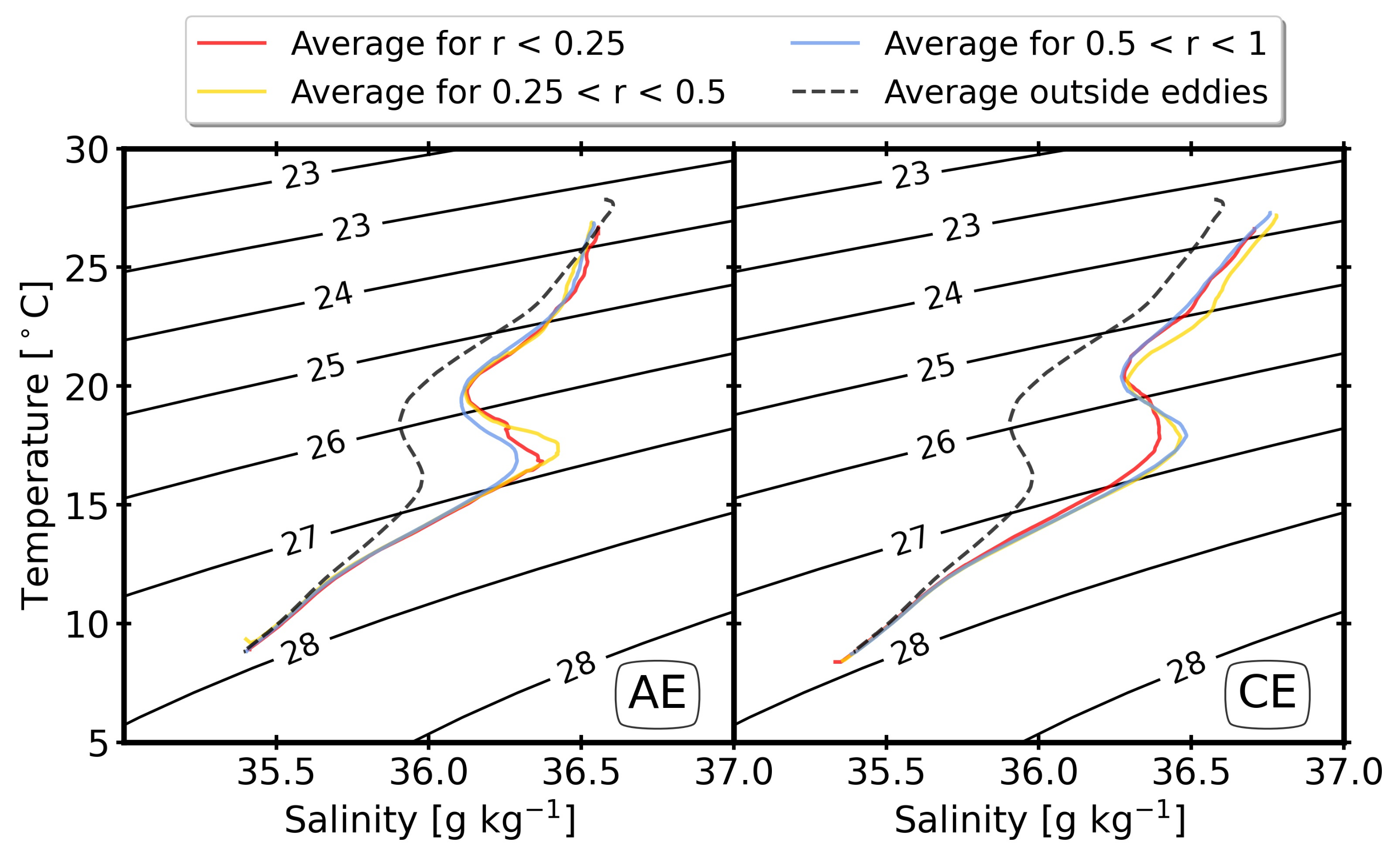
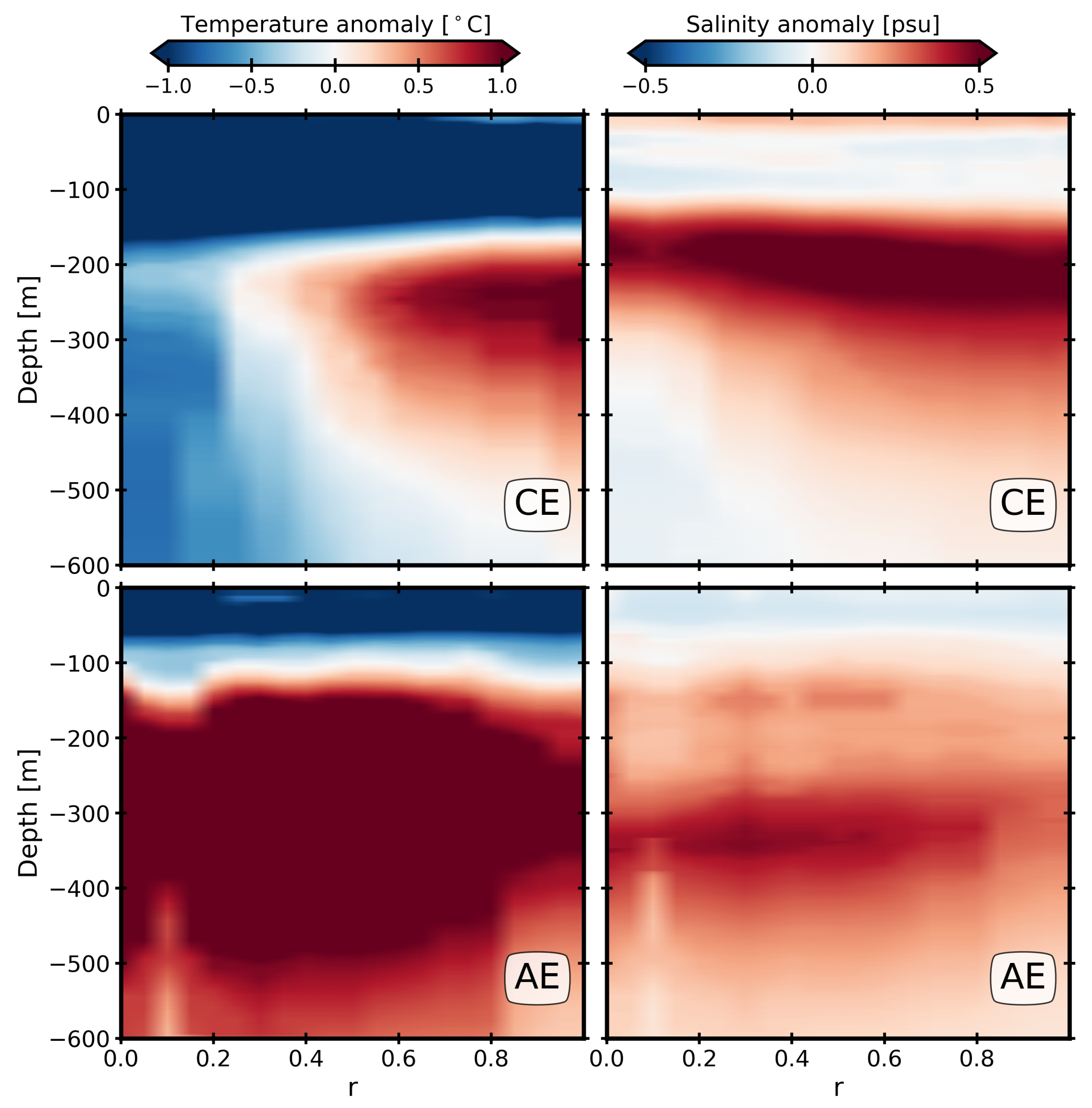
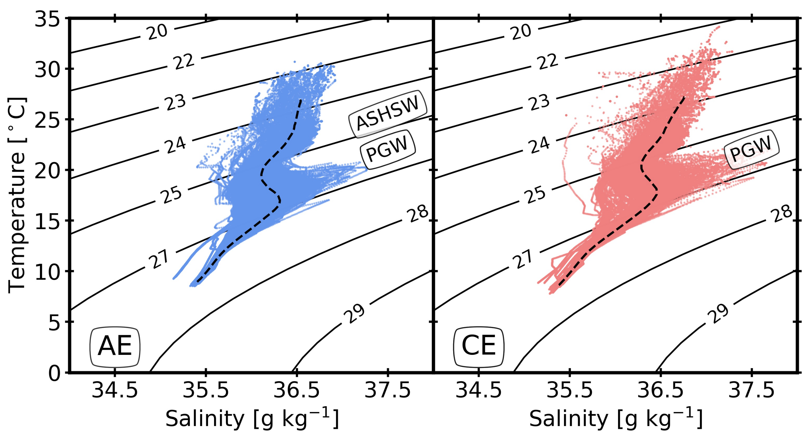
• Near the surface (top 100 m), fresh and cold waters were observed in both eddies.
• Beneath this layer (between 100 and 200 m depths), ASHSW (salty water) was found in the AE.
• In the subsurface (between 200 and 500 m), PGW (salty and warm water) was trapped in both eddies.
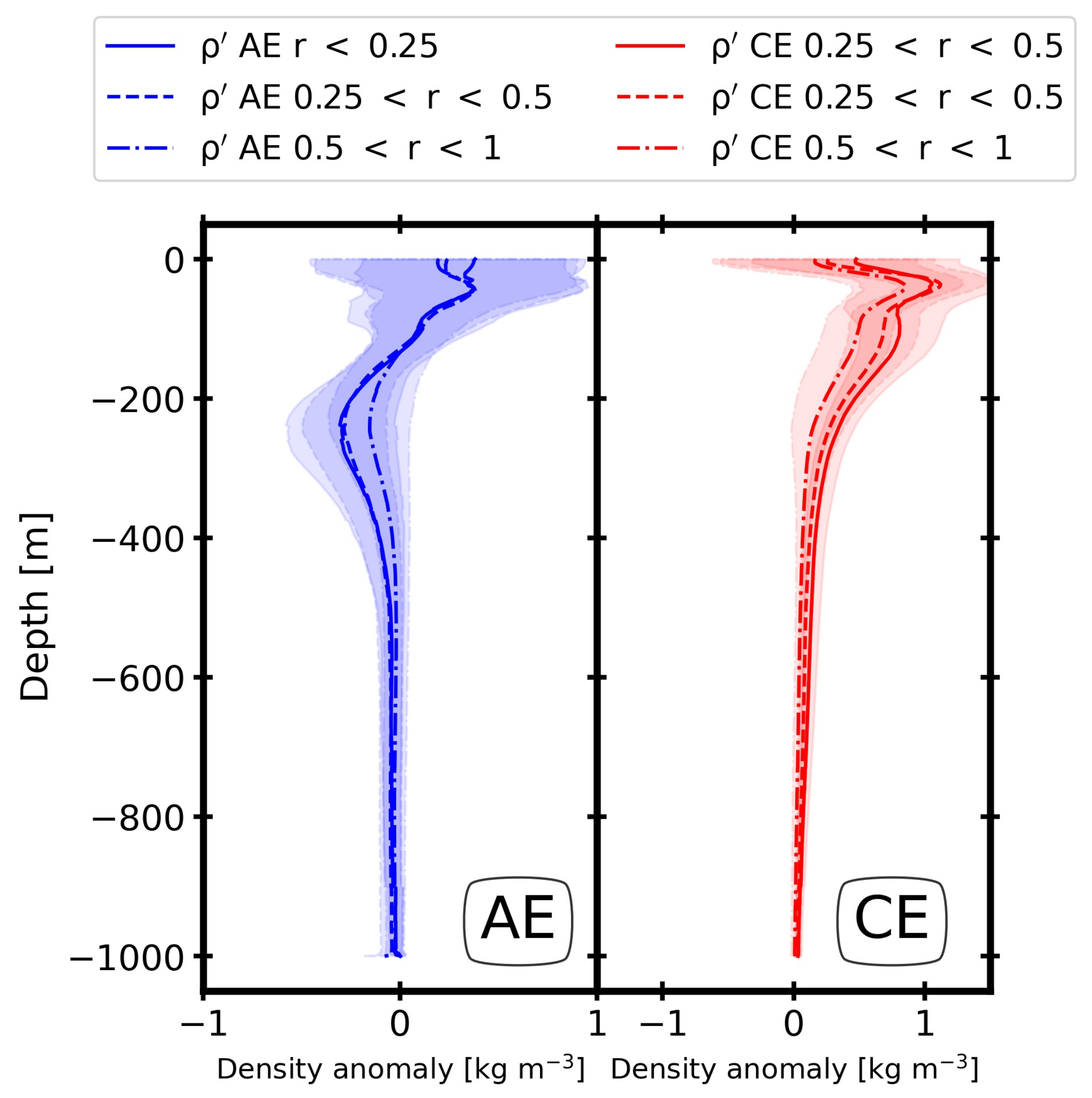
• The CE was surface-intensified and the AE was subsurface-intensified.
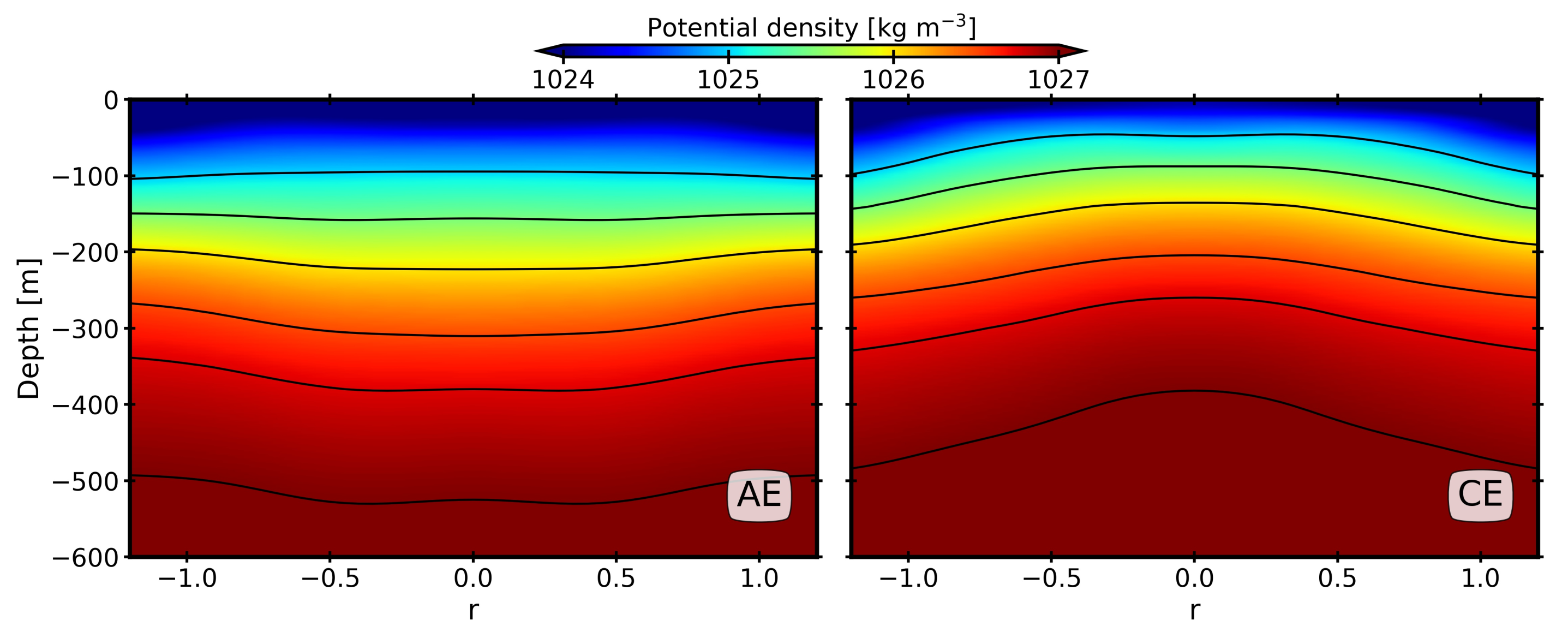
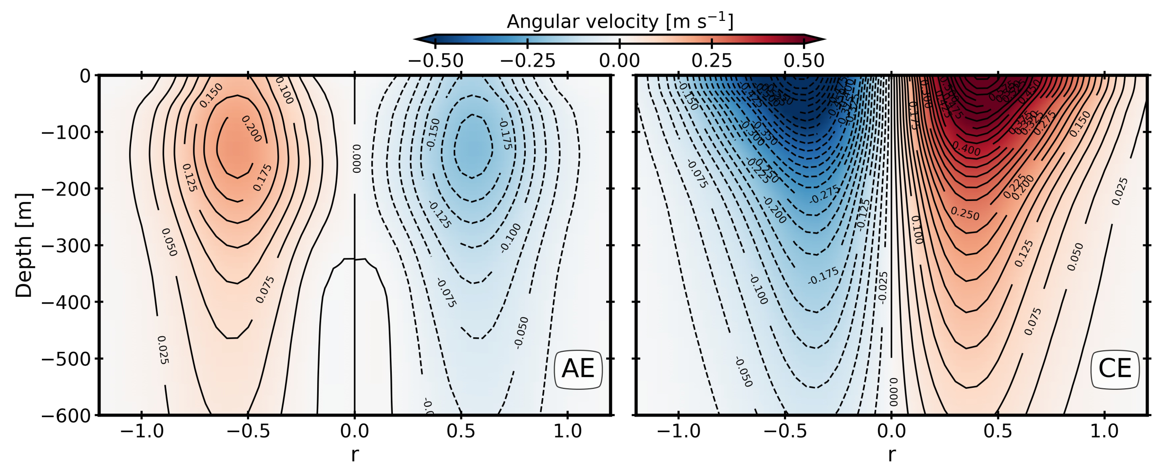
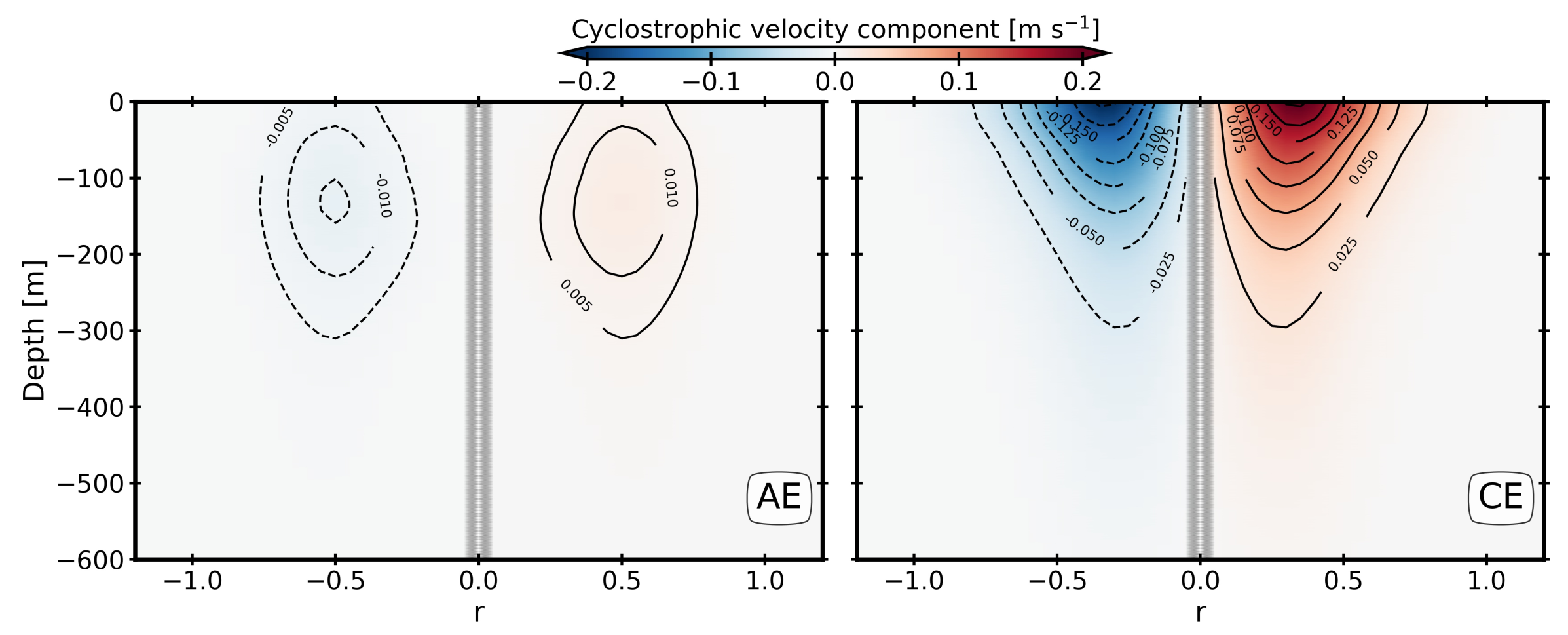
• Both eddies were Gaussian in shape; the AE was slightly larger than the CE, leading to intensification of the angular geostrophic and cyclostrophic velocities of the CE.
• The AE had a deeper signature than the CE.
• Vertical frontogenesis processes were deep-reaching in both eddies and intensified for the CE due to the surface nature and diffusive convection in its core.
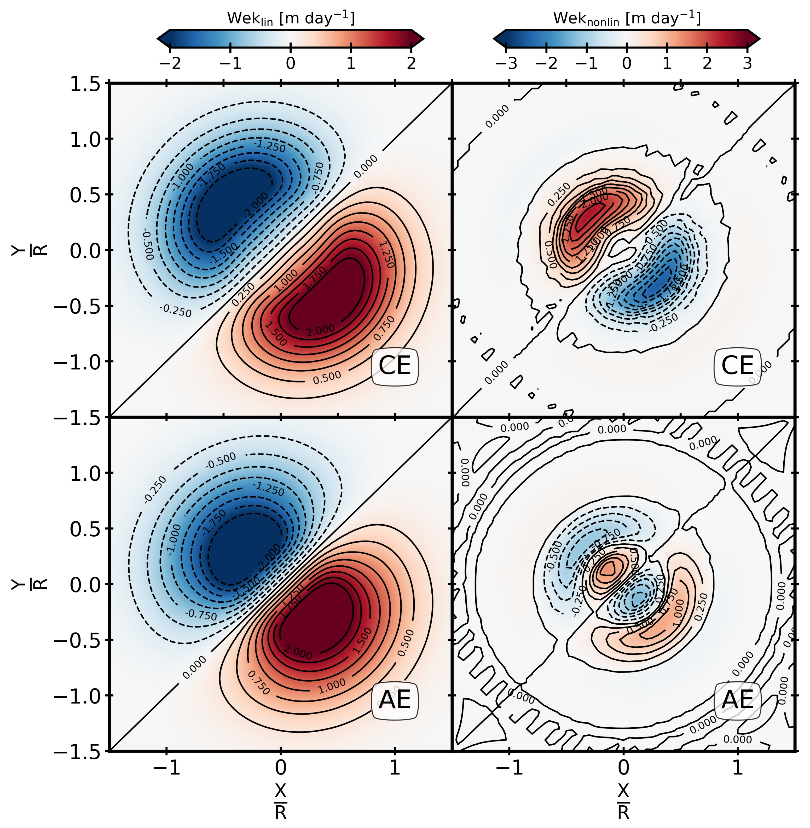
• Nonlinear and linear Ekman pumping dominated in the CE due to its stronger interaction with the atmosphere.
• Symmetric, baroclinic, and barotropic instabilities coexisted near the surface (top 200 m). They were intensified for the CE. The AE seemed to be a more stable structure.
• Our results are in good agreement with previous studies. However, a major limitation of this study is the axisymmetric assumption. This assumption does not take into consideration the distortion/deformation of eddies. The latter is important in related stratification adjustments due to potential vorticity conservation.
• Numerical modeling is necessary to examine the stability of these oceanic eddies and their interactions with winds during a long time period (a few months).

References

1. Flagg, C.N.; Kim, H.S. Upper ocean currents in the northern Arabian Sea from shipboard ADCP measurements collected during the 1994–1996 U.S. JGOFS and ONR programs. Deep Sea Res. Part II Top. Stud. Oceanogr. 1998, 45, 1917–1959. [Google Scholar] [CrossRef]
2. Wang, Z.; DiMarco, S.F.; Jochens, A.E.; Ingle, S. High salinity events in the northern Arabian Sea and Sea of Oman. Deep Sea Res. Part I Oceanogr. Res. Pap. 2013, 74, 14–24. [Google Scholar] [CrossRef]
3. De Marez, C.; L’Hégaret, P.; Morvan, M.; Carton, X. On the 3D structure of eddies in the Arabian Sea. Deep Sea Res. Part I Oceanogr. Res. Pap. 2019, 150, 103057. [Google Scholar] [CrossRef]
4. Ayouche, A.; De Marez, C.; Morvan, M.; L’Hegaret, P.; Carton, X.; Le Vu, B.; Stegner, A. Structure and Dynamics of the Ras al Hadd Oceanic Dipole in the Arabian Sea. Oceans 2021, 2, 105–125. [Google Scholar] [CrossRef]
5. Johns, W.E.; Jacobs, G.A.; Kindle, J.C.; Murray, S.P.; Carron, M. Arabian Marginal Seas and Gulfs; Technical Report; Naval Research Laboratory, Oceanography Division, Stennis Space Center: Hancock County, MS, USA, 1999. [Google Scholar]
6. Lee, C.M.; Jones, B.H.; Brink, K.H.; Fischer, A.S. The upper-ocean response to monsoonal forcing in the Arabian Sea: Seasonal and spatial variability. Deep Sea Res. Part II Top. Stud. Oceanogr. 2000, 47, 1177–1226. [Google Scholar] [CrossRef]
7. Currie, R. Circulation and upwelling off the coast of south-east Arabia. Oceanol. Acta 1992, 15, 43–60. [Google Scholar]
8. L’Hégaret, P.; de Marez, C.; Morvan, M.; Meunier, T.; Carton, X. Spreading and Vertical Structure of the Persian Gulf and Red Sea Outflows in the Northwestern Indian Ocean. J. Geophys. Res. Oceans 2021, 126, e2019JC015983. [Google Scholar] [CrossRef]
9. Emeis, K.C.; Anderson, D.M.; Doose, H.; Kroon, D.; Schulz-Bull, D. Sea-Surface Temperatures and the History of Monsoon Upwelling in the Northwest Arabian Sea during the Last 500,000 Years. Quat. Res. 1995, 43, 355–361. [Google Scholar] [CrossRef]
10. Ilicak, M.; Özgökmen, T.M.; Johns, W.E. How does the Red Sea outflow water interact with Gulf of Aden Eddies? Ocean Model. 2011, 36, 133–148. [Google Scholar] [CrossRef]
11. L’Hégaret, P.; Lacour, L.; Carton, X.; Roullet, G.; Baraille, R.; Corréard, S. A seasonal dipolar eddy near Ras Al Hamra (Sea of Oman). Ocean Dyn. 2013, 63, 633–659. [Google Scholar] [CrossRef]
12. Bower, A.S.; Hunt, H.D.; Price, J.F. Character and dynamics of the Red Sea and Persian Gulf outflows. J. Geophys. Res. Oceans 2000, 105, 6387–6414. [Google Scholar] [CrossRef]
13. Bower, A.S.; Furey, H.H. Mesoscale eddies in the Gulf of Aden and their impact on the spreading of Red Sea Outflow Water. Prog. Oceanogr. 2012, 96, 14–39. [Google Scholar] [CrossRef] [Green Version]
14. Morvan, M.; L’Hégaret, P.; de Marez, C.; Carton, X.; Corréard, S.; Baraille, R. Life cycle of mesoscale eddies in the Gulf of Aden. Geophys. Astrophys. Fluid Dyn. 2020, 114, 631–649. [Google Scholar] [CrossRef]
15. Fratantoni, D.M.; Bower, A.S.; Johns, W.E.; Peters, H. Somali Current rings in the eastern Gulf of Aden. J. Geophys. Res. Oceans 2006. [Google Scholar] [CrossRef] [Green Version]
16. Böhm, E.; Morrison, J.M.; Manghnani, V.; Kim, H.S.; Flagg, C.N. The Ras al Hadd Jet: Remotely sensed and acoustic Doppler current profiler observations in 1994–1995. Deep Sea Res. Part II Top. Stud. Oceanogr. 1999, 46, 1531–1549. [Google Scholar] [CrossRef]
17. Argo. Argo Float Data and Metadata from Global Data Assembly Centre (Argo GDAC); SEANOE: Issy-les-Moulineaux, France, 2022. [Google Scholar] [CrossRef]
18. McDougall, T.J.; Barker, P.M. Getting started with TEOS-10 and the Gibbs Seawater (GSW) oceanographic toolbox. Scor/Iapso WG 2011, 127, 1–28. [Google Scholar]
19. Vu, B.L.; Stegner, A.; Arsouze, T. Angular momentum eddy detection and tracking algorithm (AMEDA) and its application to coastal eddy formation. J. Atmos. Ocean. Technol. 2018, 35, 739–762. [Google Scholar] [CrossRef]
20. Meyers, G.; Donguy, J.R.; Bailey, R. Geostrophic Transports of the Major Current Systems in the Tropical Indian and Pacific Oceans; International WOCE Newslette, Design and Print Centre of the University of Southampton: Southampton, UK, 1996. [Google Scholar]
21. Ni, Q.; Zhai, X.; Wang, G.; Hughes, C.W. Widespread Mesoscale Dipoles in the Global Ocean. J. Geophys. Res. Oceans 2020, 125, e2020JC016479. [Google Scholar] [CrossRef]
22. Hoskins, B.J.; Draghici, I.; Davies, H.C. A new look at the ω-equation. Q. J. R. Meteorol. Soc. 1978, 104, 31–38. [Google Scholar] [CrossRef]
23. Hoskins, B.J. The role of potential vorticity in symmetric stability and instability. Q. J. R. Meteorol. Soc. 1974, 100, 480–482. [Google Scholar] [CrossRef]
24. De Marez, C.; Meunier, T.; Morvan, M.; L’Hégaret, P.; Carton, X. Study of the stability of a large realistic cyclonic eddy. Ocean Model. 2020, 146, 101540. [Google Scholar] [CrossRef]
25. Ayouche, A.; Charria, G.; Carton, X.; Ayoub, N.; Theetten, S. Non-Linear Processes in the Gironde River Plume (North-East Atlantic): Instabilities and Mixing. Front. Mar. Sci. 2021, 8, 701773. [Google Scholar] [CrossRef]
26. Ayouche, A.; Carton, X.; Charria, G.; Theettens, S.; Ayoub, N. Instabilities and vertical mixing in river plumes: Application to the Bay of Biscay. Geophys. Astrophys. Fluid Dyn. 2020, 114, 650–689. [Google Scholar] [CrossRef]
27. Laxenaire, R.; Speich, S.; Stegner, A. Evolution of the Thermohaline Structure of One Agulhas Ring Reconstructed from Satellite Altimetry and Argo Floats. J. Geophys. Res. Oceans 2019, 124, 8969–9003. [Google Scholar] [CrossRef] [Green Version]
28. Fu, L.L.; Qiu, B. Low-frequency variability of the North Pacific Ocean: The roles of boundary- and wind-driven baroclinic Rossby waves. J. Geophys. Res. Oceans 2002, 107, 13-1–13-10. [Google Scholar] [CrossRef]
29. Kumar, S.P.; Prasad, T.G. Formation and spreading of Arabian Sea high-salinity water mass. J. Geophys. Res. Oceans 1999, 104, 1455–1464. [Google Scholar] [CrossRef]
30. Assassi, C.; Morel, Y.; Vandermeirsch, F.; Chaigneau, A.; Pegliasco, C.; Morrow, R.; Colas, F.; Fleury, S.; Carton, X.; Klein, P.; et al. An index to distinguish surface- and subsurface-intensified vortices from surface observations. J. Phys. Oceanogr. 2016, 46, 2529–2552. [Google Scholar] [CrossRef]
31. Stegner, A.; Vu, B.L.; Dumas, F.; Ghannami, M.A.; Nicolle, A.; Durand, C.; Faugere, Y. Cyclone-Anticyclone Asymmetry of Eddy Detection on Gridded Altimetry Product in the Mediterranean Sea. J. Geophys. Res. Oceans 2021, 126, e2021JC017475. [Google Scholar] [CrossRef]
32. Roullet, G.; Klein, P. Cyclone-Anticyclone Asymmetry in Geophysical Turbulence. Phys. Rev. Lett. 2010, 104, 218501. [Google Scholar] [CrossRef]
33. Chu, X.; Chen, G.; Qi, Y. Periodic Mesoscale Eddies in the South China Sea. J. Geophys. Res. Oceans 2019, 125, e2019JC015139. [Google Scholar] [CrossRef]
34. Pilo, G.S.; Oke, P.R.; Coleman, R.; Rykova, T.; Ridgway, K. Patterns of Vertical Velocity Induced by Eddy Distortion in an Ocean Model. J. Geophys. Res. Oceans 2018, 123, 2274–2292. [Google Scholar] [CrossRef]
35. Gaube, P.; Chelton, D.B.; Samelson, R.M.; Schlax, M.G.; O’Neill, L.W. Satellite observations of mesoscale eddy-induced Ekman pumping. J. Phys. Oceanogr. 2015, 45, 104–132. [Google Scholar] [CrossRef]
36. Wang, Y.; Zhang, H.R.; Chai, F.; Yuan, Y. Impact of mesoscale eddies on chlorophyll variability off the coast of Chile. PLoS ONE 2018, 13, 1–13. [Google Scholar] [CrossRef]
37. Cornec, M.; Laxenaire, R.; Speich, S.; Claustre, H. Impact of Mesoscale Eddies on Deep Chlorophyll Maxima. Geophys. Res. Lett. 2021, 48, e2021GL093470. [Google Scholar] [CrossRef]
Figure 2. Average distribution of the ARGO float positions inside eddies (figure at the top) and average distribution of the ARGO float positions outside eddies (figure at the bottom) for the different months of the year. Regarding the top figure, there are two distinct censuses for the AC and for the AE. The number (#) in the y axis of this figure refers to the number of colocalized ARGO floats.
Oceans 03 00019 g002
Figure 3. Distribution of the inside/outside eddy profiles in the NAS region, which includes the Gulf of Oman and the northern part of the Arabian Sea (called area D).
Oceans 03 00019 g003
Figure 4. TS-diagram of the RAH dipole located in the NAS area for the CE and AC, bold solid lines are iso-density lines, the PGW signature is found in the CE and both PGW and ASHSW in the AC.
Oceans 03 00019 g004
Figure 5. Averaged TS-diagram for both AE (left) and CE (right) regions; black dashed lines indicate the average outside eddies; the three colored lines indicate the respective average positions of the float to the center of the eddy.
Oceans 03 00019 g005
Figure 6. Density anomaly profiles, for both eddies of the RAH; AE/CE, several types of traits represent the different positions of the ARGO float detected inside the eddies; continuous line for profiles near the center r < 0.25; dashed line for further profiles 0.25 < r < 0.5; mixed line for the profiles near the edges 0.5 < r < 1.
Oceans 03 00019 g006
Figure 7. The 3D structure of the AE and CE temperature anomaly and salinity anomaly for a grid of depth and the location of the ARGO floats inside the eddies. These anomalies are smoothed using a median filter of a kernel size of 8.
Oceans 03 00019 g007
Figure 8. The 3D structure of the potential densities of AC and CE (as a function of the depth). The CE potential density curves obtained above 500 m depth are concave and symmetrical for radii between −1 and 1 and the potential density curves obtained are slightly straight above 200 m in depth while for depths between 200 and 500 m they are convex.
Oceans 03 00019 g008
Figure 9. The angular velocity for the AE and CE. Solid and dashed contours indicate positive and negative values, respectively.
Oceans 03 00019 g009
Figure 10. The cyclostrophic component for the CE and AE. Dashed and solid contours indicate negative and positive values, respectively.
Oceans 03 00019 g010
Figure 11. Density anomaly amplitude versus depth; the blue lines represent the AE amplitude and the CE is presented in red. The eddy depths are represented by black circles.
Oceans 03 00019 g011
Figure 12. (a): Variation CE and AE radii. Figure (b): Steepness parameter α . Figure (c): Potential density RMSE error. The different figures are presented for three depth classes; the blue bars represent the AE and the red bars the CE.
Oceans 03 00019 g012
Figure 13. Sea level anomaly for the AE and CE of RAH.
Oceans 03 00019 g013
Figure 14. The geostrophic velocity components U g and V g of the CE and AE.
Oceans 03 00019 g014
Figure 15. Frontogenesis vertical velocity averaged between the surface and 400 m for the CE and AE. Dashed and solid contours represent negative and positive values with steps of 0.5 for the CE and 0.2 for the AE.
Oceans 03 00019 g015
Figure 16. The vertical pumping velocity due to the linear and nonlinear Ekman components during the northeastern monsoon.
Oceans 03 00019 g016
Figure 17. Maxima of the nonlinear (dashed) and linear (solid) Ekman pumping for the CE (red) and the AE (blue), in regards to the magnitude of the wind stress.
Oceans 03 00019 g017
Figure 18. The horizontal component of the EPV for the CE and AE.
Oceans 03 00019 g018
Figure 19. The vertical component of the EPV for the CE and AE.
Oceans 03 00019 g019
Figure 20. The horizontal component of the EPV anomaly for the CE and AE.
Oceans 03 00019 g020
Figure 21. The vertical component of the EPV anomaly for the CE and AE.
Oceans 03 00019 g021