
On the Seasonal Dynamics of Phytoplankton Chlorophyll-a Concentration in Nearshore and Offshore Waters of Plymouth, in the English Channel: Enlisting the Help of a Surfer


 ,
,  , ,
, ,  ,
,
Abstract
:
1. Introduction
- Is the seasonal cycle of chl-a significantly different between a nearshore and offshore coastal location in Plymouth, UK?
- Is the relationship between chl-a and the physical environment significantly different between these two nearshore and offshore locations?
- Is there a difference in how phytoplankton are limited at these two nearshore and offshore locations?
2. Methodology
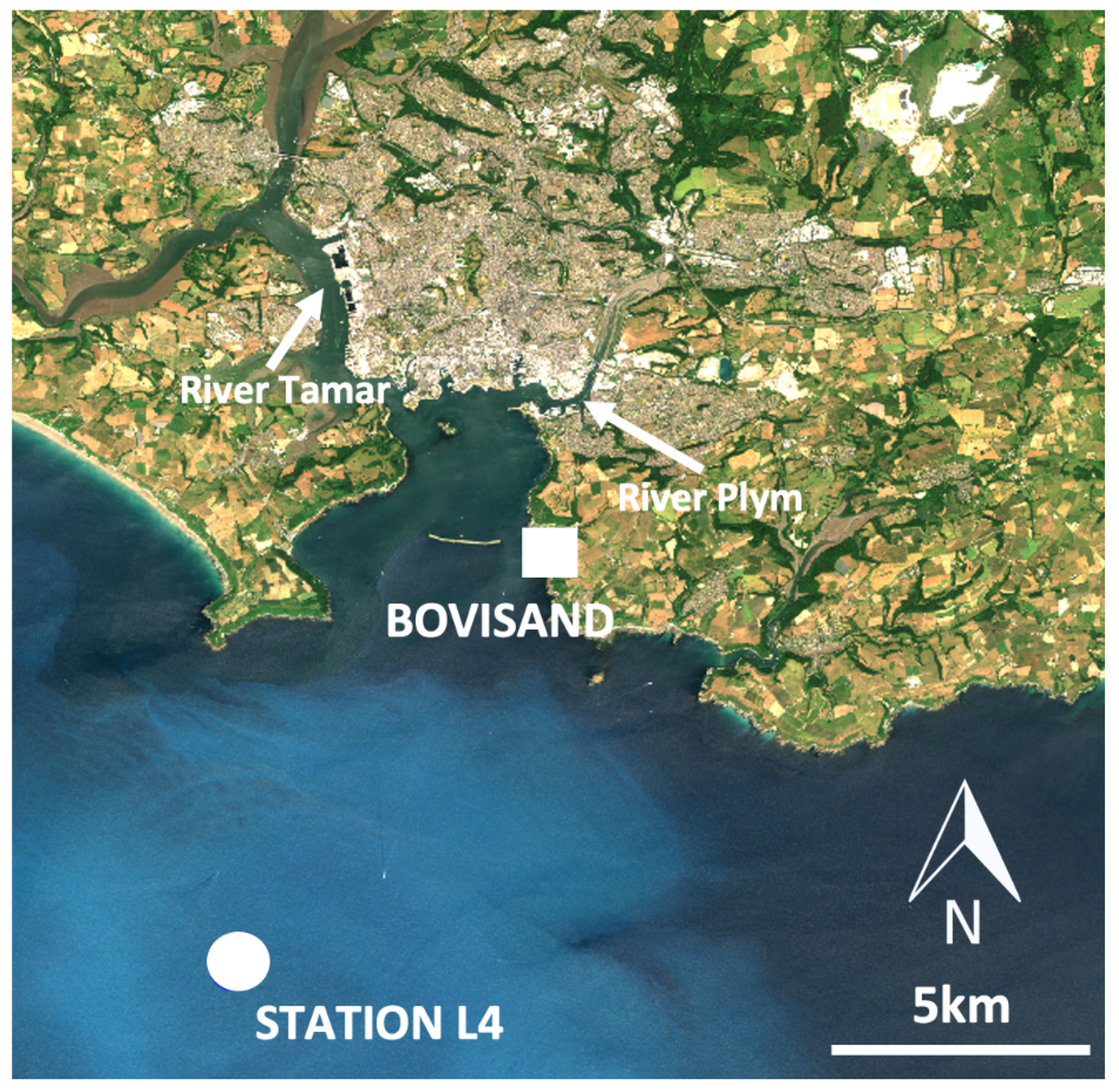
2.1. Study Area
2.2. Data Acquisition
2.2.1. Bovisand In-Situ Data
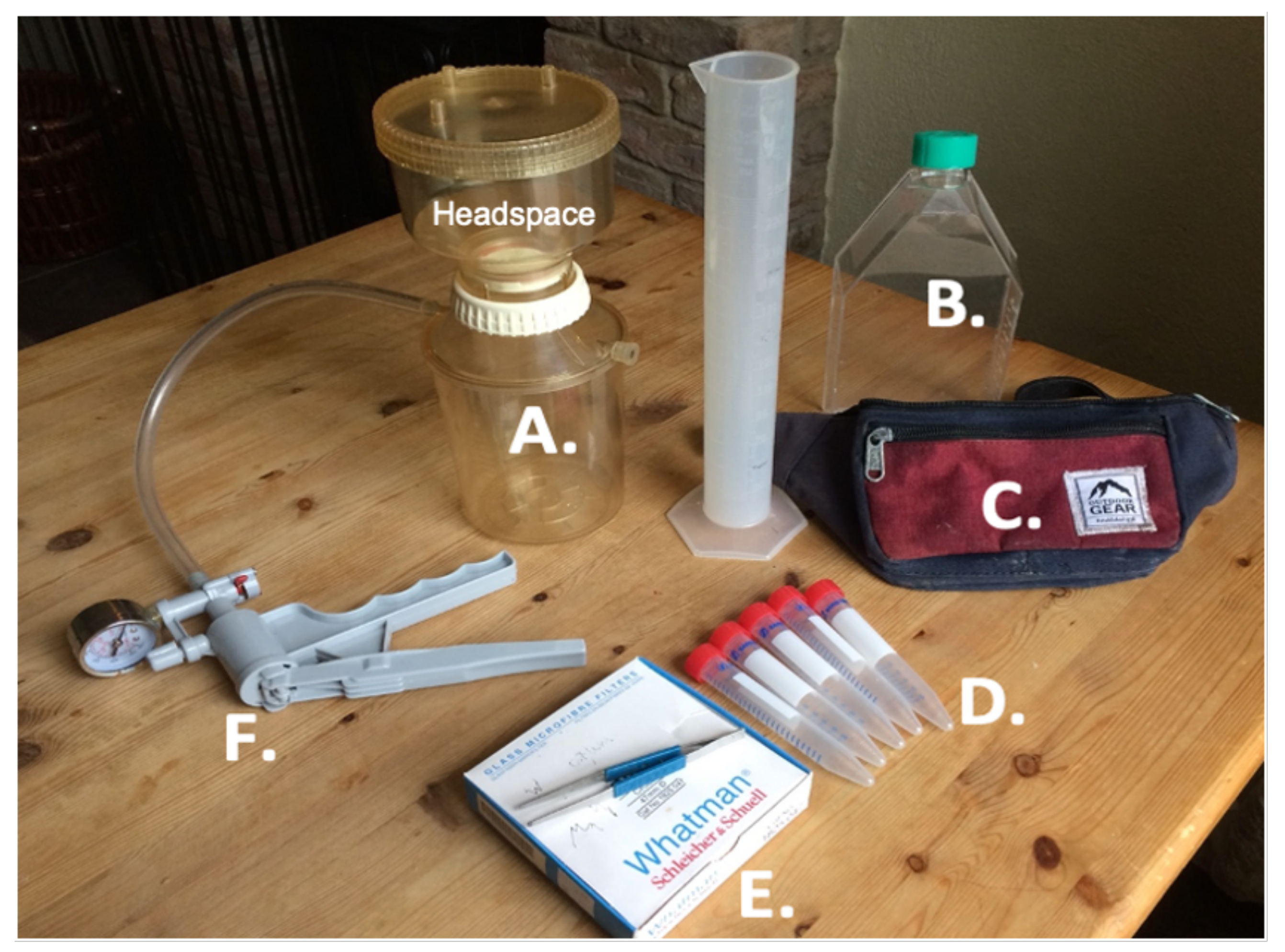
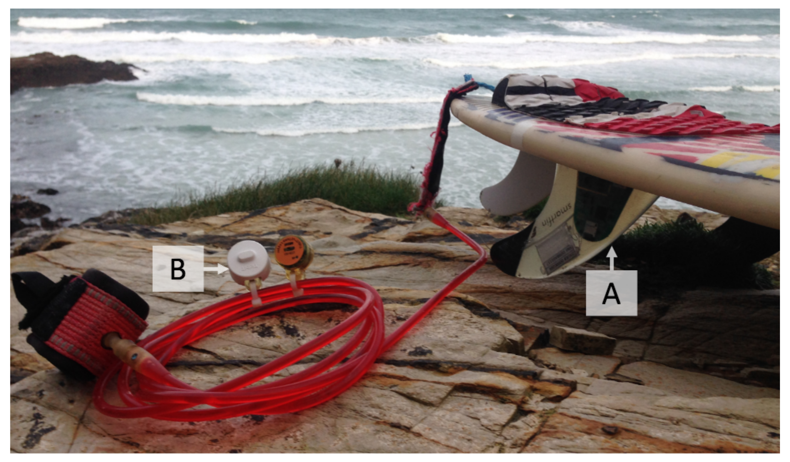
Sample Collection
Sample Preparation and Fluorometric Analysis
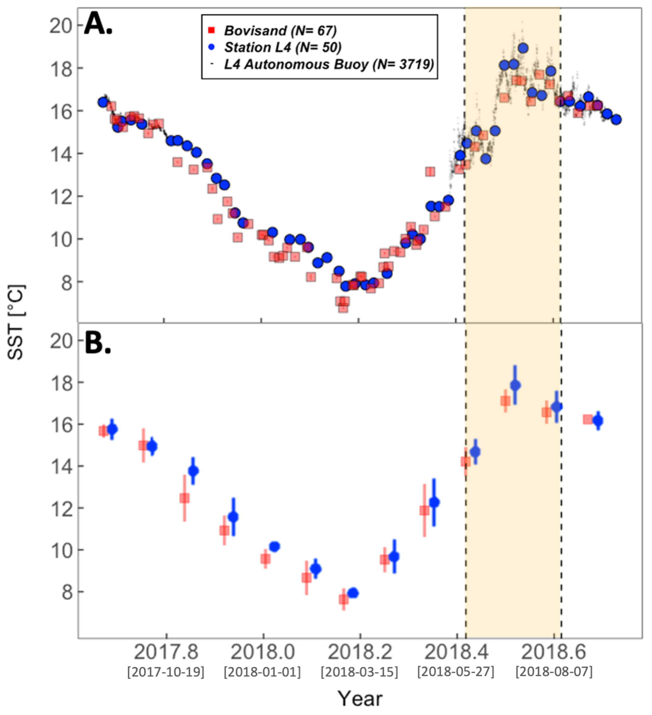
Sea Surface Temperature (SST) at the Beach
2.2.2. Station L4 In-Situ Data
2.2.3. Auxiliary Data
L4 Autonomous Buoy
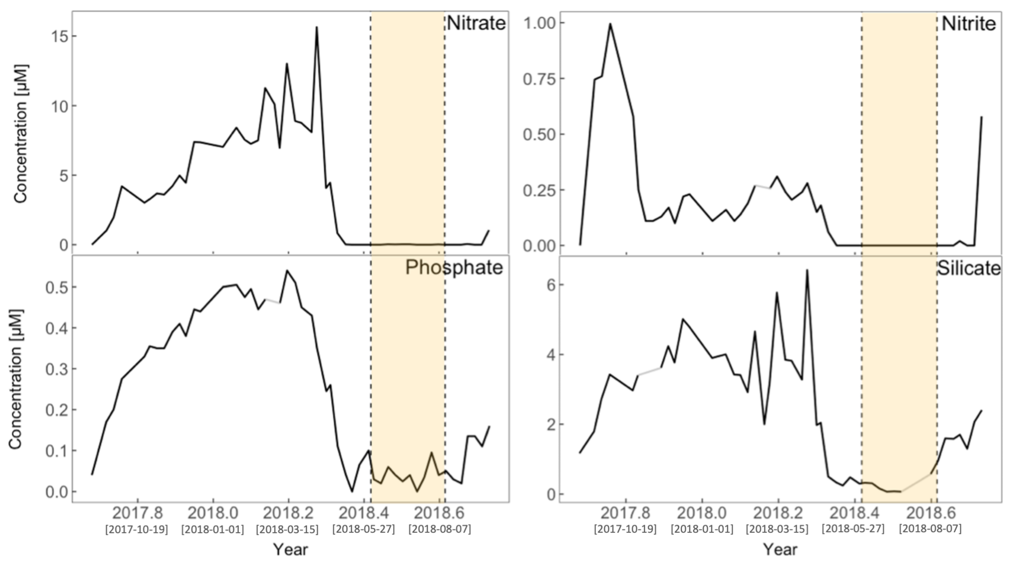
Surface Nutrients
Stratification
Microscopy Data
Satellite Data
2.2.4. Calculating chl-a Uncertainty
2.2.5. Statistical Analysis
3. Results
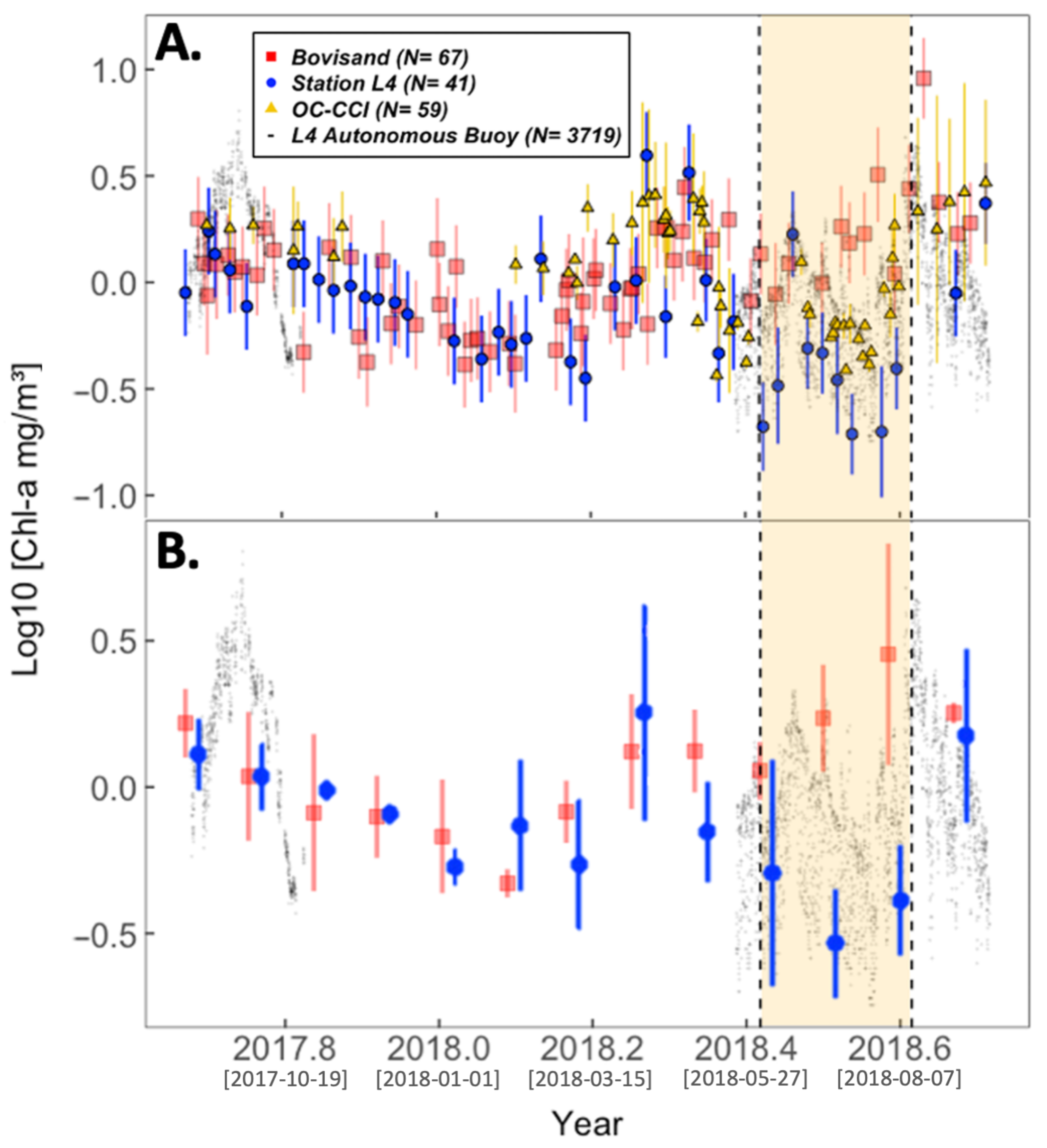
3.1. Seasonal Cycle of chl-a
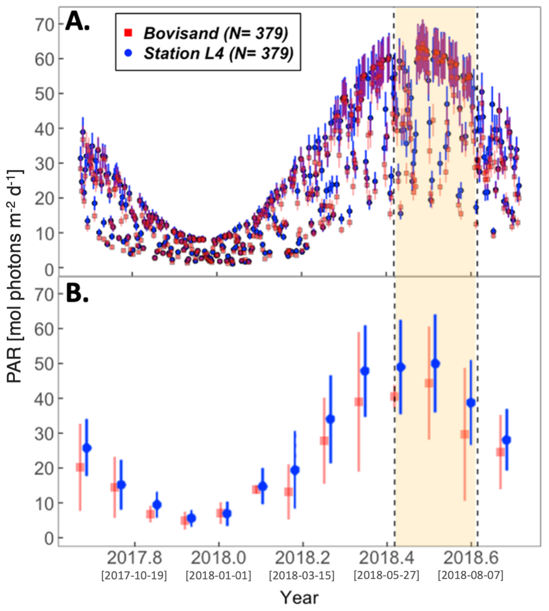
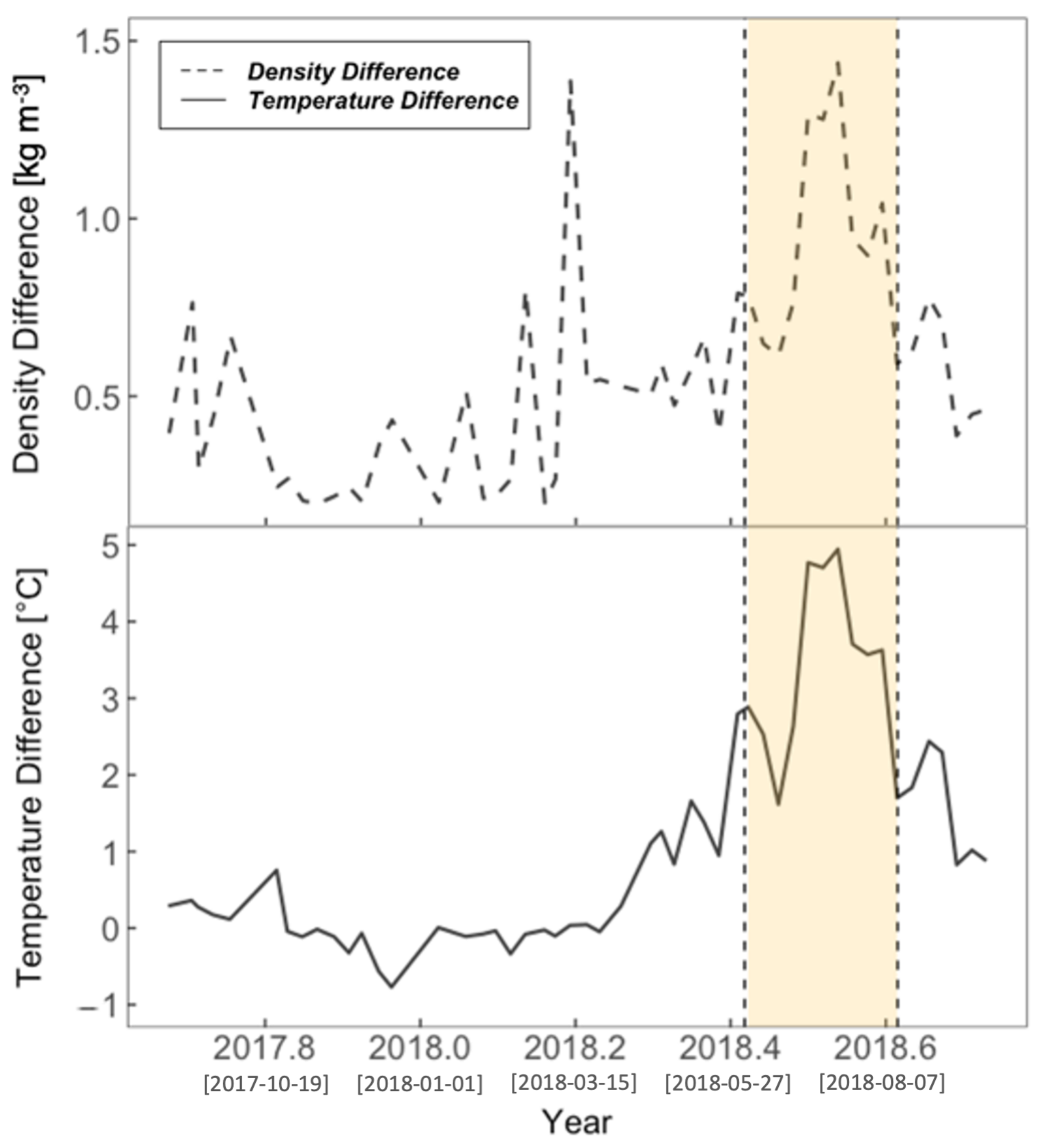
3.2. Physical Environment Time Series
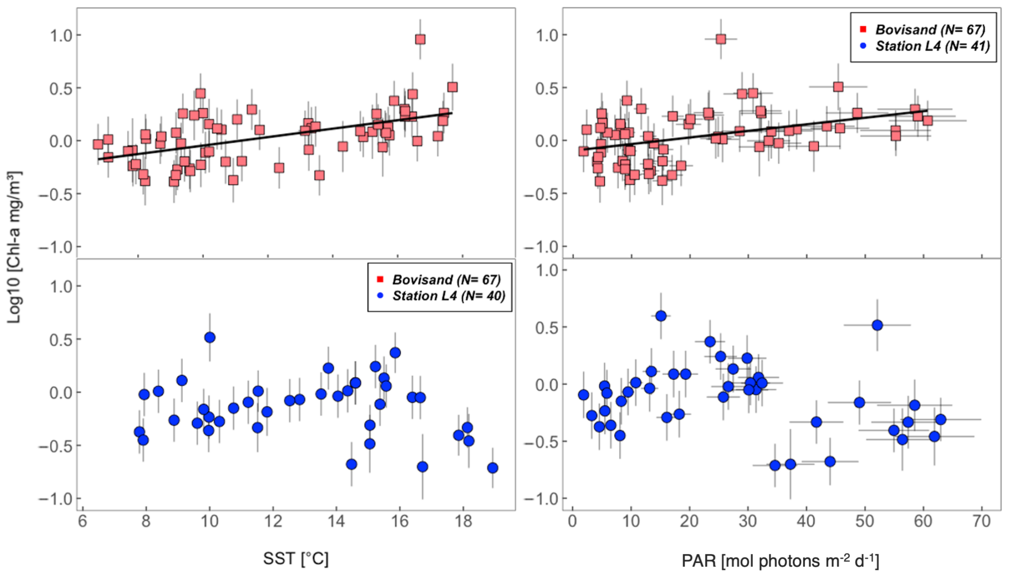
3.3. Relationships between chl-a and the Physical Environment
4. Discussion
4.1. Research Questions
4.2. Nearshore-Offshore: Why the Difference?
4.3. Implications for Understanding Coastal Phytoplankton Dynamics
4.4. Limitations of Our Study
4.5. Future Directions
5. Conclusions
Author Contributions
Funding
Data Availability Statement
Acknowledgments
Conflicts of Interest
References
- Litchman, E.; de Tezanos Pinto, P.; Edwards, K.; Klausmeier, C.; Kremer, C.; Thomas, M. Global Biogeochemical Impacts of Phytoplankton: A Trait-Based Perspective. J. Ecol. 2015, 103, 1384–1396. [Google Scholar] [CrossRef] [Green Version]
- Fox, J.; Behrenfeld, M.; Haëntjens, N.; Chase, A.; Kramer, S.; Boss, E.; Karp-Boss, L.; Fisher, N.; Penta, W.; Westberry, T.; et al. Phytoplankton Growth and Productivity in the Western North Atlantic: Observations of Regional Variability from the NAAMES Field Campaigns. Front. Mar. Sci. 2020, 7, 1–15. [Google Scholar] [CrossRef]
- Longhurst, A.; Sathyendranath, S.; Platt, T.; Caverhill, C. An estimate of global primary production in the ocean from satellite radiometer data. J. Plankton Res. 1995, 17, 1245–1271. [Google Scholar] [CrossRef] [Green Version]
- Field, C.B.; Behrenfeld, M.J.; Randerson, J.T.; Falkowski, P.G. Primary production of the biosphere: Integrating terrestrial and oceanic components. Science 1998, 281, 237–240. [Google Scholar] [CrossRef] [Green Version]
- Duarte, C.; Cebrián, J. The Fate of Marine Autotrophic Production. Limnol. Oceanogr. 1996, 41, 1758–1766. [Google Scholar] [CrossRef]
- Takahashi, T.; Sutherland, S.C.; Sweeney, C.; Poisson, A.; Metzl, N.; Tilbrook, B.; Bates, N.; Wanninkhof, R.; Feely, R.A.; Sabine, C.; et al. Global sea–air CO2 flux based on climatological surface ocean pCO2, and seasonal biological and temperature effects. Deep Sea Res. Part II Top. Stud. Oceanogr. 2002, 49, 1601–1622. [Google Scholar] [CrossRef]
- Yang, X.; Liu, L.; Yin, Z.; Wang, X.; Wang, S.; Ye, Z. Quantifying Photosynthetic Performance of Phytoplankton Based on Photosynthesis-Irradiance Response Models. Environ. Sci. Eur. 2020, 32, 1–13. [Google Scholar] [CrossRef] [Green Version]
- Hecky, R.; Campbell, P.; Hendzel, L. The stoichiometry of carbon, nitrogen, and phosphorus in particulate matter of lakes and oceans. Limnol. Oceanogr. 1993, 38, 709–724. [Google Scholar] [CrossRef]
- Hutchins, D.; Wang, W.; Fisher, N. Copepod grazing and the biogeochemical fate of diatom iron. Limnol. Oceanogr. 1995, 40, 989–994. [Google Scholar] [CrossRef]
- Geider, R.; Delucia, E.; Falkowski, P.; Finzi, A.; Grime, J.; Grace, J.; Kana, T.; La Roche, J.; Long, S.; Osborne, B.; et al. Primary productivity of planet Earth: Biological determinants and physical constraints in terrestrial and aquatic habitats. Glob. Chang. Biol. 2001, 7, 849–882. [Google Scholar] [CrossRef]
- Moore, C.; Mills, M.; Arrigo, K.; Berman-Frank, I.; Bopp, L.; Boyd, P.; Galbraith, E.; Geider, R.; Guieu, C.; Jaccard, S.; et al. Processes and patterns of oceanic nutrient limitation. Nat. Geosci. 2013, 6, 701–710. [Google Scholar] [CrossRef] [Green Version]
- Calbet, A.; Landry, M. Phytoplankton growth, microzooplankton grazing, and carbon cycling in marine systems. Limnol. Oceanogr. 2004, 49, 51–57. [Google Scholar] [CrossRef] [Green Version]
- Schmoker, C.; Hernández-León, S.; Calbet, A. Microzooplankton grazing in the oceans: Impacts, data variability, knowledge gaps and future directions. J. Plankton Res. 2013, 35, 691–706. [Google Scholar] [CrossRef]
- Agustí, S.; Satta, M.P.; Mura, M.P.; Benavent, E. Dissolved esterase activity as a tracer of phytoplankton lysis: Evidence of high phytoplankton lysis rates in the northwestern Mediterranean. Limnol. Oceanogr. 1998, 43, 1836–1849. [Google Scholar] [CrossRef]
- Sverdrup, H. On conditions for the vernal blooming of phytoplankton. J. Cons. Perm. Int. Explor. Mer 1953, 18, 287–295. [Google Scholar] [CrossRef]
- Behrenfeld, M.J.; O’Malley, R.T.; Siegel, D.A.; McClain, C.R.; Sarmiento, J.L.; Feldman, G.C.; Milligan, A.J.; Falkowski, P.G.; Letelier, R.M.; Boss, E.S. Climate-driven trends in contemporary ocean productivity. Nature 2006, 444, 752–755. [Google Scholar] [CrossRef]
- Martinez, E.; Antoine, D.; D’Ortenzio, F.; Gentili, B. Climate-driven basin-scale decadal oscillations of oceanic phytoplankton. Science 2009, 3261, 253–1256. [Google Scholar] [CrossRef] [Green Version]
- Winder, M.; Cloern, J. The annual cycles of phytoplankton biomass. Philos. Trans. R. Soc. B Biol. Sci. 2010, 365, 3215–3226. [Google Scholar] [CrossRef]
- Brewin, R.J.W.; Hirata, T.; Hardman-Mountford, N.J.; Lavender, S.; Sathyendranath, S.; Barlow, R. The influence of the Indian Ocean Dipole on interannual variations in phytoplankton size structure as revealed by Earth Observation. Deep Sea Res. II 2012, 77–80, 117–127. [Google Scholar] [CrossRef]
- Racault, M.F.; Le Quéré, C.; Buitenhuis, E.; Sathyendranath, S.; Platt, T. Phytoplankton phenology in the global ocean. Ecol. Indic. 2012, 14, 152–163. [Google Scholar] [CrossRef]
- Racault, M.F.; Raitsos, D.E.; Berumen, M.L.; Brewin, R.J.W.; Platt, T.; Sathyendranath, S.; Hoteit, I. Phytoplankton phenology indices in coral reef ecosystems: Application to ocean-colour observations in the Red Sea. Remote Sens. Environ. 2015, 160, 222–234. [Google Scholar] [CrossRef] [Green Version]
- Racault, M.F.; Sathyendranath, S.; Brewin, R.J.W.; Raitsos, D.; Jackson, T.; Platt, T. Impact of El Nino Variability on Oceanic Phytoplankton. Front. Mar. Sci. 2017, 4, 133. [Google Scholar] [CrossRef] [Green Version]
- Bolaños, L.; Karp-Boss, L.; Choi, C.; Worden, A.; Graff, J.; Haëntjens, N.; Chase, A.; Della Penna, A.; Gaube, P.; Morison, F.; et al. Small phytoplankton dominate western North Atlantic biomass. ISME J. 2020, 14, 1663–1674. [Google Scholar] [CrossRef] [PubMed] [Green Version]
- Slade, W.H.; Boss, E.; Dall’Olmo, G.; Langner, M.R.; Loftin, J.; Behrenfeld, M.J.; Roesler, C.; Westberry, T.K. Underway and moored methods for improving accuracy in measurement of spectral particulate absorption and attenuation. J. Atmos. Ocean. Technol. 2010, 27, 1733–1746. [Google Scholar] [CrossRef]
- Dall’Olmo, G.; Boss, E.; Behrenfeld, M.; Westberry, T.K. Particulate optical scattering coefficients along an Atlantic Meridional Transect. Opt. Express 2012, 20, 21532–21551. [Google Scholar] [CrossRef]
- Leeuw, T.; Boss, E.; Wright, D. In situ measurements of phytoplankton fluorescence using low cost electronics. Sensors 2013, 13, 7872–7883. [Google Scholar] [CrossRef] [Green Version]
- Roesler, C.; Barnard, A.H. Optical proxy for phytoplankton biomass in the absence of photophysiology: Rethinking the absorption line height. Methods Oceanogr. 2013, 7, 79–94. [Google Scholar] [CrossRef]
- Brewin, R.J.W.; Dall’Olmo, G.; Pardo, S.; van Dongen-Vogel, V.; Boss, E.S. Underway spectrophotometry along the Atlantic Meridional Transect reveals high performance in satellite chlorophyll retrievals. Remote Sens. Environ. 2016, 183, 82–97. [Google Scholar] [CrossRef] [Green Version]
- Blauw, A.; Benincá, E.; Laane, R.; Greenwood, N.; Huisman, J. Predictability and environmental drivers of chlorophyll fluctuations vary across different time scales and regions of the North Sea. Prog. Oceanogr. 2018, 161, 1–18. [Google Scholar] [CrossRef]
- Graban, S.; Dall’Olmo, G.; Goult, S.; Sauzéde, R. Accurate deep-learning estimation of chlorophyll-a concentration from the spectral particulate beam-attenuation coefficient. Opt. Express 2020, 28, 24214–24228. [Google Scholar] [CrossRef]
- Claustre, H.; Johnson, K.S.; Takeshita, Y. Observing the Global Ocean with Biogeochemical-Argo. Annu. Rev. Mar. Sci. 2020, 12, 23–48. [Google Scholar] [CrossRef]
- Chai, F.; Johnson, K.S.; Claustre, H.; Xing, X.; Wang, Y.; Boss, E.; Riser, S.; Fennel, K.; Schofield, O.; Sutton, A. Monitoring ocean biogeochemistry with autonomous platforms. Nat. Rev. Earth Environ. 2020, 1, 315–326. [Google Scholar] [CrossRef]
- Zaneveld, J.R.V.; Barnard, A.H.; Boss, E. Theoretical derivation of the depth average of remotely sensed optical parameters. Opt. Express 2005, 13, 9052–9061. [Google Scholar] [CrossRef] [Green Version]
- Brewin, R.J.W.; Sathyendranath, S.; Müller, D.; Brockmann, C.; Deschamps, P.Y.; Devred, E.; Doerffer, R.; Fomferra, N.; Franz, B.A.; Grant, M.; et al. The Ocean Colour Climate Change Initiative: III. A round-robin comparison on in-water bio-optical algorithms. Remote Sens. Environ. 2015, 162, 271–294. [Google Scholar] [CrossRef] [Green Version]
- Groom, S.; Sathyendranath, S.; Ban, Y.; Bernard, S.; Brewin, R.J.W.; Brotas, V.; Brockmann, C.; Chauhan, P.; Choi, J.; Chuprin, A.; et al. Satellite Ocean Colour: Current Status and Future Perspective. Front. Mar. Sci. 2019, 6, 485. [Google Scholar] [CrossRef] [Green Version]
- Sathyendranath, S.; Brewin, R.J.W.; Brockmann, C.; Brotas, V.; Calton, B.; Chuprin, A.; Cipollini, P.; Couto, A.B.; Dingle, J.; Doerffer, R.; et al. An Ocean-Colour Time Series for Use in Climate Studies: The Experience of the Ocean-Colour Climate Change Initiative (OC-CCI). Sensors 2019, 19, 4285. [Google Scholar] [CrossRef] [Green Version]
- Jickells, T.D. Nutrient biogeochemistry of the coastal zone. Science 1998, 281, 217–222. [Google Scholar] [CrossRef]
- Tittensor, D.P.; Mora, C.; Jetz, W.; Lotze, H.K.; Ricard, D.; Berghe, E.V.; Worm, B. Global patterns and predictors of marine biodiversity across taxa. Nature 2010, 466, 1098–1101. [Google Scholar] [CrossRef]
- Costanza, R.; d’Arge, R.; de Groot, R.; Farberk, S.; Grasso, M.; Hannon, B.; Limburg, K.; Naeem, S.; O’Neill, R.V.; Paruelo, J.; et al. The value of the world’s ecosystem services and natural capital. Nature 1997, 387, 253–260. [Google Scholar] [CrossRef]
- Andersson, A.J.; Mackenzie, F.T. Shallow-water ocean: A source or sink of atmospheric CO2? Front. Ecol. Environ. 2004, 2, 348–353. [Google Scholar] [CrossRef]
- Mackenzie, F.T.; Andersson, A.J.; Lerman, A.; Ver, L.M. Boundary exchanges in the global coastal margin: Implications for the organic and inorganic carbon cycles. In The Sea, Vol. 13, The Global Coastal Ocean: Multiscale Interdiciplinary Processes; Robinson, A.R., Brink, K., Eds.; Harvard University Press: Cambridge, MA, USA, 2005. [Google Scholar]
- Stewart, K.R.; Lewison, R.L.; Dunn, D.C.; Borkland, R.H.; Kelez, S.; Halpin, P.N.; Crowder, L.B. Characterizing fishing effort and spatial extent of coastal fisheries. PLoS ONE 2010, 5, e14451. [Google Scholar] [CrossRef] [Green Version]
- IOCCG. Remote Sensing of Ocean Colour in Coastal, and Other Optically Complex Waters; Technical Report; Reports of the International Ocean-Colour Coordinating Group, No. 3; Sathyendranath, S., Ed.; IOCCG: Dartmouth, NS, Canada, 2000. [Google Scholar]
- Feng, L.; Hu, C. Land adjacency effects on MODIS Aqua top-of-atmosphere radiance in the shortwave infrared: Statistical assessment and correction. J. Geophys. Res. Ocean. 2017, 122, 4802–4818. [Google Scholar] [CrossRef]
- Frouin, R.J.; Franz, B.A.; Ibrahim, A.; Knobelspiesse, K.; Ahmad, Z.; Cairns, B.; Chowdhary, J.; Dierssen, H.M.; Tan, J.; Dubovik, O.; et al. Atmospheric Correction of Satellite Ocean-Color Imagery During the PACE Era. Front. Earth Sci. 2019, 7, 145. [Google Scholar] [CrossRef] [Green Version]
- Brewin, R.J.W.; Hyder, K.; Andersson, A.J.; Billson, O.; Bresnahan, P.J.; Brewin, T.G.; Cyronak, T.; Dall’Olmo, G.; de Mora, L.; Graham, G.; et al. Expanding aquatic observations through recreation. Front. Mar. Sci. 2017, 4, 351. [Google Scholar] [CrossRef] [Green Version]
- Brewin, R.J.W.; de Mora, L.; Jackson, T.; Brewin, T.G.; Shutler, J. On the potential of surfers to monitor environmental indicators in the coastal zone. PLoS ONE 2015, 10, e0127706. [Google Scholar] [CrossRef]
- Brewin, R.J.W.; de Mora, L.; Billson, O.; Jackson, T.; Russell, P.; Brewin, T.G.; Shutler, J.; Miller, P.I.; Taylor, B.H.; Smyth, T.; et al. Evaluating operational AVHRR sea surface temperature data at the coastline using surfers. Estuarine Coast. Shelf Sci. 2017, 196, 276–289. [Google Scholar] [CrossRef]
- Vanhellemont, Q.; Brewin, R.J.W.; Bresnahan, P.; Cyronak, T. Validation of Landsat 8 high resolution Sea Surface Temperature using surfers. Estuar. Coast. Shelf Sci. 2022, 265, 107650. [Google Scholar] [CrossRef]
- Bresnahan, P.J.; Cyronak, T.; Martz, T.; Andersson, A.; Waters, S.; Stern, A.; Richard, J.; Hammond, K.; Griffin, J.; Thompson, B. Engineering a Smartfin for surf-zone oceanography. In Proceedings of the OCEANS 2017—Anchorage, Anchorage, AK, USA, 18–21 September 2017; pp. 1–4. [Google Scholar]
- Bresnahan, P.; Cyronak, T.; Brewin, R.J.W.; Andersson, A.; Wirth, T.; Martz, T.; Courtney, T.; Hui, N.; Kastner, R.; Stern, A.; et al. A high-tech, low-cost, Internet of Things surfboard fin for coastal citizen science, outreach, and education. Cont. Shelf Res. 2022. in review. [Google Scholar]
- Brewin, R.J.W.; Cyronak, T.; Bresnahan, P.J.; Andersson, A.J.; Richard, J.; Hammond, K.; Billson, O.; de Mora, L.; Jackson, T.; Smale, D.; et al. Comparison of two methods for measuring sea surface temperature when surfing. Oceans 2020, 1, 2. [Google Scholar] [CrossRef] [Green Version]
- Brewin, R.J.W.; Wimmer, W.; Bresnahan, P.J.; Cyronak, T.; Andersson, A.J.; Dall’Olmo, G. Comparison of a Smartfin with an infrared sea surface temperature radiometer in the Atlantic Ocean. Remote Sens. 2021, 13, 841. [Google Scholar] [CrossRef]
- Wright, S.; Hull, T.; Sivyer, D.B.; Pearce, D.; Pinnegar, J.K.; Sayer, M.D.J.; Mogg, A.O.M.; Azzopardi, E.; Gontarek, S.; Hyder, K. SCUBA divers as oceanographic samplers: The potential of dive computers to augment aquatic temperature monitoring. Sci. Rep. 2016, 6, 30164. [Google Scholar] [CrossRef] [Green Version]
- Egi, S.; Cousteau, P.Y.; Pieri, M.; Cerrano, C.; Özyigit, T.; Marroni, A. Designing a Diving Protocol for Thermocline Identification Using Dive Computers in Marine Citizen Science. Appl. Sci. 2018, 8, 2315. [Google Scholar] [CrossRef] [Green Version]
- Marlowe, C.; Hyder, K.; Sayer, M.D.J.; Kaiser, J. Divers as citizen scientists: Response time, accuracy and precision of water temperature measurement using dive computers. Front. Mar. Sci. 2021, 8, 617691. [Google Scholar] [CrossRef]
- Bresnahan, P.J.; Wirth, T.; Martz, T.R.; Andersson, A.J.; Cyronak, T.; D’Angelo, S.; Pennise, J.; Melville, W.K.; Lenain, L.; Statom, N. A sensor package for mapping pH and oxygen from mobile platforms. Methods Oceanogr. 2016, 17, 1–13. [Google Scholar] [CrossRef] [Green Version]
- Griffiths, A.G.F.; Kemp, K.M.; Matthews, K.; Garrett, J.K.; Griffiths, D.J. Sonic Kayaks: Environmental monitoring and experimental music by citizens. PLoS Biol. 2017, 15, e2004044. [Google Scholar] [CrossRef] [Green Version]
- Griffiths, A.G.; Garrett, J.K.; Duffy, J.P.; Matthews, K.; Visi, F.G.; Eatock, C.; Robinson, M.; Griffiths, D.J. New water and air pollution sensors added to the Sonic Kayak citizen science system for low cost environmental mapping. J. Open Hardw. 2021, 5, 1–5. [Google Scholar] [CrossRef]
- Lauro, F.M.; Senstius, S.J.; Cullen, J.; Neches, R.; Jensen, R.M.; Brown, M.V.; Darling, A.E.; Givskov, M.; McDougald, D.; Hoeke, R.; et al. The Common Oceanographer: Crowdsourcing the Collection of Oceanographic Data. PLoS Biol. 2014, 12, e1001947. [Google Scholar] [CrossRef] [Green Version]
- Seafarers, S.D.; Lavender, S.; Beaugrand, G.; Outram, N.; Barlow, N.; Crotty, D.; Evans, J.; Kirby, R. Seafarer citizen scientist ocean transparency data as a resource for phytoplankton and climate research. PLoS ONE 2017, 12, e0186092. [Google Scholar] [CrossRef] [Green Version]
- Brewin, R.J.W.; Brewin, T.G.; Phillips, J.; Rose, S.; Abdulaziz, A.; Wimmer, W.; Sathyendranath, S.; Platt, T. A Printable Device for Measuring Clarity and Colour in Lake and Nearshore Waters. Sensors 2019, 19, 936. [Google Scholar] [CrossRef] [Green Version]
- Menon, N.; George, G.; Ranith, R.; Sajin, V.; Murali, S.; Abdulaziz, A.; Brewin, R.J.W.; Sathyendranath, S. Citizen science tools reveal changes in estuarine water quality following demolition of buildings. Remote Sens. 2021, 13, 1683. [Google Scholar] [CrossRef]
- George, G.; Menon, N.N.; Abdulaziz, A.; Brewin, R.J.W.; Pranav, P.; Gopalakrishnan, A.; Mini, K.G.; Kuriakose, S.; Sathyendranath, S.; Platt, T. Citizen scientists contribute to real-time monitoring of lake water quality using 3D printed mini Secchi disks. Front. Water 2021, 3, 662142. [Google Scholar] [CrossRef]
- Kirby, R.R.; Beaugrand, G.; Kleparski, L.; Goodall, S.; Lavender, S. Citizens and scientists collect comparable oceanographic data: Measurements of ocean transparency from the Secchi Disk study and science programmes. Sci. Rep. 2021, 11, 15499. [Google Scholar] [CrossRef]
- Menge, B.A.; Daley, B.A.; Wheeler, P.A.; Strub, P.T. Rocky intertidal oceanography: An association between community structure and nearshore phytoplankton concentration. Limnol. Oceanogr. 2003, 42, 57–66. [Google Scholar] [CrossRef] [Green Version]
- O’Boyle, S.; Silke, J. A review of phytoplankton ecology in estuarine and coastal waters around Ireland. J. Plankton Res. 2009, 32, 99–118. [Google Scholar] [CrossRef] [Green Version]
- Schaeffer, B.A.; Kurtz, J.C.; Hein, M.K. Phytoplankton community composition in nearshore coastal waters of Louisiana. Mar. Pollut. Bull. 2012, 64, 1705–1712. [Google Scholar] [CrossRef]
- Zohdi, E.; Abbaspour, M. Harmful algal blooms (red tide): A review of causes, impacts and approaches to monitoring and prediction. Int. J. Environ. Sci. Technol. 2019, 16, 1789–1806. [Google Scholar] [CrossRef]
- Depew, D.; Guildford, S.; Smith, R. Nearshore-offshore comparison of chlorophyll-a and phytoplankton production in the dreissenid-colonized Eastern Basin of Lake Erie. Can. J. Fish. Aquat. Sci. 2006, 63, 1115–1129. [Google Scholar] [CrossRef]
- Guildford, S. Nearshore-offshore differences in planktonic chlorophyll and phytoplankton nutrient status after dreissenid establishment in a large shallow lake. Inland Waters 2013, 3, 253–268. [Google Scholar] [CrossRef]
- Kovalenko, K.; Reavie, E.; Bramburger, A.; Cotter, A.; Sierszen, M. Nearshore-offshore trends in Lake Superior phytoplankton. J. Great Lakes Res. 2019, 45, 1197–1204. [Google Scholar] [CrossRef]
- Wang, Y.; Gao, Z. Contrasting chlorophyll-a seasonal patterns between nearshore and offshore waters in the Bohai and Yellow Seas, China: A new analysis using improved satellite data. Cont. Shelf Res. 2020, 203, 1–15. [Google Scholar] [CrossRef]
- Smyth, T.J.; Fishwick, J.; Al-Moosawi, L.; Cummings, D.G.; Harris, R.; Kitidis, V.; Rees, A.; Martinez-Vicente, V.; Woodward, E.M.S. A broad spatio-temporal view of the Western English Channel observatory. J. Plankton Res. 2010, 32, 585–601. [Google Scholar] [CrossRef] [Green Version]
- Smyth, T.J.; Fishwick, J.R.; Gallienne, C.P.; Stephens, J.A.; Bale, A.J. Technology, design, and operation of an autonomous buoy system in the Western English Channel. J. Atmos. Ocean. Technol. 2010, 27, 2056–2064. [Google Scholar] [CrossRef]
- Western Channel Observatory Main Data Page. Available online: https://www.westernchannelobservatory.org.uk/data.php (accessed on 2 May 2021).
- EPA. Standard Operating Procedure for Chlorophyll a Sampling Method Field Procedure; Technical Report; United States Environmental Protection Agency: Washington, DC, USA, 2013.
- Nayar, S.; Chou, L. Relative efficiencies of different filters in retaining phytoplankton for pigment and productivity studies. Estuarine Coast. Shelf Sci. 2003, 58, 241–248. [Google Scholar] [CrossRef]
- Saldanha-Corrêa, F.; Gianesella, S.; Barrera-Alba, J. A comparison of the retention capability among three different glass-fibre filters used for chlorophyll-a determinations. Braz. J. Oceanogr. 2004, 52, 243–247. [Google Scholar] [CrossRef]
- Wasmund, N.; Schories, D. Optimising the storage and extraction of chlorophyll samples. Oceanologia 2006, 48, 125–144. [Google Scholar]
- Arar, E.; Collins, G. Method 455.0 In Vitro Determination of Chlorophyll a and Pheophytin a in Marine and Freshwater Algae by Fluorescence; Technical Report; U.S. Environmental Protection Agency: Washington, DC, USA, 1997.
- Welschmeyer, N. Fluorometric analysis of chlorophyll a in the presence of chlorophyll b and pheopigments. Limnol. Oceanogr. 1994, 39, 1985–1992. [Google Scholar] [CrossRef]
- McCluskey, E.; Brewin, R.J.W.; Jones, O.; Cummings, D.; Tilstone, G.; Bresnahan, P.J.; Cyronak, T.; Andersson, A. An Annual Time-Series of Chlorophyll-a and Sea Surface Temperature Measurements Collected between 2017 and 2018 by a Surfer at Bovisand Beach, Plymouth, UK; NERC EDS British Oceanographic Data Centre NOC. 2022. Available online: https://www.bodc.ac.uk/data/published_data_library/catalogue/10.5285/d6a5a863-a43d-28a9-e053-6c86abc0b1f4/ (accessed on 1 October 2020).
- Western Channel Observatory L4 In-Situ Data Station. Available online: https://www.westernchannelobservatory.org.uk/l4_ctdf/index.php (accessed on 1 October 2020).
- Sea-Bird Electronics. SBE 19plus SeaCAT Profiler CTD User Manual; Technical Report; Sea-Bird Scientific: Washington, DC, USA, 2016. [Google Scholar]
- Western Channel Observatory L4 Autonomous Buoy. Available online: https://www.westernchannelobservatory.org.uk/buoys.php (accessed on 1 October 2020).
- Baker, N. Chlorophyll fluorescence: A probe of photosynthesis in vivo. Annu. Rev. Plant Biol. 2008, 59, 89–113. [Google Scholar] [CrossRef] [Green Version]
- Xing, X.; Morel, A.; Claustre, H.; D’Orenzio, F.; Poteau, A.; Mignot, A. Combined processing and mutual interpretation of radiometry and fluorometry from autonomous profiling Bio-Argo floats: 2. Colored dissolved organic matter absorption retrieval. J. Geophys. Res. 2012, 117, C04022. [Google Scholar] [CrossRef] [Green Version]
- Western Channel Observatory L4 Surface Nutrients Data. Available online: https://www.westernchannelobservatory.org.uk/l4_nutrients.php (accessed on 8 March 2021).
- Widdicombe, C.; Eloire, D.; Harbour, D.; Harris, R.; Somerfield, P. Long-term phytoplankton community dynamics in the Western English Channel. J. Plankton Res. 2010, 32, 643–655. [Google Scholar] [CrossRef] [Green Version]
- Throndsen, J. Preservation and storage. In Phytoplankton Manual; Sournia, A., Ed.; UNESCO: Paris, France, 1978; pp. 69–74. [Google Scholar]
- Utermohl, H. Vervollkommung der quantitativen Phytoplankton-Methodik. Mitt. Internationalen Verein Limnologie 1958, 9, 1–38. [Google Scholar]
- BS EN 15204:2006; Water Quality—Guidance Standard on the Enumeration of Phytoplankton Using Inverted Microscopy (Utermohl Technique). European Standard: Pilsen, Czech Republic, 2006.
- Gould, R., Jr.; Ko, D.; Ladner, S.; Lawson, T.; MacDonald, C. Comparison of Satellite, Model, and In Situ Values of Photosynthetically Available Radiation (PAR). J. Atmos. Ocean. Technol. 2019, 36, 535–555. [Google Scholar] [CrossRef]
- NASA Ocean Color Chlorophyll (OC) v6. Available online: https://oceancolor.gsfc.nasa.gov/reprocessing/r2009/ocv6/ (accessed on 10 December 2021).
- Campbell, J.W. The lognormal distribution as a model for bio-optical variability in the sea. J. Geophys. Res. 1995, 100, 13237–13254. [Google Scholar] [CrossRef]
- Claustre, H.; Hooker, S.B.; Van Heukelem, L.; Berthon, J.F.; Barlow, R.; Ras, J.; Sessions, H.; Targa, C.; van der Linde, D.; Marty, J.C. An intercomparison of HPLC phytoplankton pigment methods using in situ samples: Application to remote sensing and database activities. Mar. Chem. 2004, 85, 41–61. [Google Scholar] [CrossRef]
- Lindemann, C.; St. John, M.; St. A seasonal diary of phytoplankton in the North Atlantic. Front. Mar. Sci. 2014, 1, 1–37. [Google Scholar] [CrossRef] [Green Version]
- Litchman, E. Resource Competition and the Ecological Success of Phytoplankton. In Evolution of Primary Producers in the Sea; Falkowski, P.G., Knol, A.H., Eds.; Academic Press: Cambridge, MA, USA, 2007; pp. 351–375. [Google Scholar]
- Evans, G.; Parslow, J. A model of annual plankton cycles. Biol. Oceanogr. 1985, 3, 327–347. [Google Scholar] [CrossRef]
- Townsend, D.; Keller, M.; Sieracki, M.; Ackleson, S. Spring phytoplankton blooms in the absence of vertical water column stratification. Nature 1992, 360, 59–62. [Google Scholar] [CrossRef]
- Backhaus, J.; Hegseth, E.; Wehde, H.; Irigoien, X.; Hatten, K.; Logemann, K. Convection and primary production in winter. Mar. Ecol. Prog. Ser. 2003, 251, 1–14. [Google Scholar] [CrossRef] [Green Version]
- Sakshaug, E.; Johnsen, G.; Andresen, K.; Vernet, M. Modeling of light-dependent algal photosynthesis and growth: Experiments with the Barents sea diatoms Thalassiosira nordenskioldii and Chaetoceros furcellatus. Deep Sea Res. Part A Oceanogr. Res. Pap. 1991, 38, 415–430. [Google Scholar] [CrossRef]
- Ward, B.; Waniek, J. Phytoplankton growth conditions during autumn and winter in the Irminger Sea, North Atlantic. Mar. Ecol. Prog. Ser. 2007, 334, 47–61. [Google Scholar] [CrossRef]
- Mignot, A.; Ferrari, R.; Claustre, H. Floats with bio-optical sensors reveal what processes trigger the North Atlantic bloom. Nat. Commun. 2018, 9, 190. [Google Scholar] [CrossRef] [Green Version]
- Li, G.; Cheng, L.; Zhu, J.; Trenberth, K.; Mann, M.; Abraham, J. Increasing ocean stratification over the past half-century. Nat. Clim. Chang. 2020, 10, 1116–1123. [Google Scholar] [CrossRef]
- Lozier, M.; Dave, A.; Palter, J.; Gerber, L.; Barber, R. On the relationship between stratification and primary productivity in the North Atlantic. Geophys. Res. Lett. 2011, 38, 1–6. [Google Scholar] [CrossRef] [Green Version]
- Uncles, R.J.; Fraser, A.I.; Butterfield, D.; Johnes, P.; Harrod, T.R. The prediction of nutrients into estuaries and their subsequent behaviour: Application to the Tamar and comparison with the Tweed, U.K. In Nutrients and Eutrophication in Estuaries and Coastal Waters. Developments in Hydrobiology; Orive, E., Elliott, M., de Jonge, V.N., Eds.; Springer: Dordrecht, The Netherlands, 2002; Volume 164. [Google Scholar] [CrossRef]
- Desmit, X.; Thieu, V.; Billen, G.; Campuzano, F.; Dulière, V.; Garnier, J.; Lassaletta, L.; Ménesguen, A.; Neves, R.; Pinto, L.; et al. Reducing marine eutrophication may require a paradigmatic change. Sci. Total Environ. 2018, 635, 1444–1466. [Google Scholar] [CrossRef]
- Fredston-Hermann, A.; Brown, C.; Albert, S.; Klein, C.; Mangubhai, S.; Nelson, J.; Teneva, L.; Wenger, A.; Gaines, S.; Halpern, B. Where does river runoff matter for coastal marine conservation? Front. Mar. Sci. 2016, 3, 273. [Google Scholar] [CrossRef] [Green Version]
- Savage, C.; Leavitt, P.; Elmgren, R. Effects of land use, urbanization, and climate variability on coastal eutrophication in the Baltic Sea. Limnol. Oceanogr. 2010, 55, 1033–1046. [Google Scholar] [CrossRef]
- Drupp, P.; De Carlo, E.; Mackenzie, F.; Bienfang, P.; Sabine, C. Nutrient inputs, phytoplankton response, and CO2 variations in a semi-enclosed subtropical embayment, Kaneohe Bay, Hawaii. Aquat. Geochem. 2011, 17, 473–498. [Google Scholar] [CrossRef]
- Winder, M.; Sommer, U. Phytoplankton response to a changing climate. Hydrobiologia 2012, 698, 5–16. [Google Scholar] [CrossRef]
- Capotondi, A.; Alexander, M.; Bond, N.; Curchitser, E.; Scott, J. Enhanced upper ocean stratification with climate change in the CMIP3 models. J. Geophys. Res. Ocean. 2012, 117, C04031. [Google Scholar] [CrossRef]
- Behrenfeld, M.; Doney, S.; Lima, I.; Boss, E.; Siegel, D. Annual cycles of ecological disturbance and recovery underlying the subarctic Atlantic spring plankton bloom. Glob. Biogeochem. Cycles 2013, 27, 526–540. [Google Scholar] [CrossRef] [Green Version]
- Griffith, A.; Gobler, C. Harmful algal blooms: A climate change co-stressor in marine and freshwater ecosystems. Harmful Algae 2020, 91, 101590. [Google Scholar] [CrossRef]
- Sathyendranath, S.; Brewin, R.J.W.; Jackson, T.; Mélin, F.; Platt, T. Ocean-Colour Products for Climate-Change Studies: What are their ideal characteristics? Remote Sens. Environ. 2017, 203, 125–138. [Google Scholar] [CrossRef] [Green Version]
- Fernand, L.; Weston, K.; Morris, T.; Greenwood, N.; Brown, J.; Jickells, T. The contribution of the deep chlorophyll maximum to primary production in a seasonally stratified shelf sea, the North Sea. Biogeochemistry 2013, 113, 153–166. [Google Scholar] [CrossRef]
- Weston, K.; Fernand, L.; Mills, D.; Delahunty, R.; Brown, J. Primary production in the deep chlorophyll maximum of the central North Sea. J. Plankton Res. 2005, 27, 909–922. [Google Scholar] [CrossRef] [Green Version]
- Barnett, M.; Kemp, A.; Hickman, A.; Purdie, D. Shelf sea subsurface chlorophyll maximum thin layers have a distinct phytoplankton community structure. Cont. Shelf Res. 2019, 174, 140–157. [Google Scholar] [CrossRef]
- Moeller, H.; Laufkötter, C.; Sweeney, E.; Johnson, M. Light-Dependent Grazing Can Drive Formation and Deepening of Deep Chlorophyll Maxima. Nat. Commun. 2019, 10, 1978. [Google Scholar] [CrossRef]
- IOCCG. Phytoplankton Functional Types from Space; Technical Report; Reports of the International Ocean-Colour Coordinating Group, No. 15; Sathyendranath, S., Ed.; IOCCG: Dartmouth, NS, Canada, 2014. [Google Scholar]
- Fedak, M.A. The impact of animal platforms on polar ocean observation. Deep Sea Res. Part II Top. Stud. Oceanogr. 2013, 88, 7–13. [Google Scholar] [CrossRef]
- Harcourt, R.; Sequeira, A.M.M.; Zhang, X.; Roquet, F.; Komatsu, K.; Heupel, M.; McMahon, C.; Whoriskey, F.; Meekan, M.; Carroll, G.; et al. Animal-Borne Telemetry: An Integral Component of the Ocean Observing Toolkit. Front. Mar. Sci. 2019, 6, 326. [Google Scholar] [CrossRef] [Green Version]
- Keates, T.R.; Kudela, R.M.; Holser, R.R.; Hückstädt, L.A.; Simmons, S.E.; Costa, D.P. Chlorophyll fluorescence as measured in situ by animal-borne instruments in the northeastern Pacific Ocean. J. Mar. Syst. 2020, 203, 103265. [Google Scholar] [CrossRef]
- Alderkamp, A.; Mills, M.; van Dijken, G.; Arrigo, K. Photoacclimation and non-photochemical quenching under in situ irradiance in natural phytoplankton assemblages from the Amundsen Sea, Antarctica. Mar. Ecol. Prog. Ser. 2013, 475, 15–34. [Google Scholar] [CrossRef] [Green Version]
- Clark, D.; Feddersen, F.; Omand, M.; Guza, R. Measuring fluorescent dye in the bubbly and sediment-laden surfzone. Water Air Soil Pollut. 2009, 204, 103–115. [Google Scholar] [CrossRef] [Green Version]
- Omand, M.; Feddersen, F.; Clark, D.; Franks, P.; Leichter, J.; Guza, R. Influence of bubbles and sand on chlorophyll-a fluorescence measurements in the surfzone. Limnol. Oceanogr. Methods 2009, 7, 354–362. [Google Scholar] [CrossRef]
- Sabbah, S.; Fraser, J.; Boss, E.; Blum, I.; Hawryshyn, C. Hyperspectral portable beam transmissometer for the ultraviolet-visible spectrum. Limnol. Oceanogr. Methods 2010, 8, 527–538. [Google Scholar] [CrossRef] [Green Version]
- Bushinsky, S.M.; Takeshita, Y.; Williams, N.L. Observing Changes in Ocean Carbonate Chemistry: Our Autonomous Future. Curr. Clim. Chang. Rep. 2019, 5, 207–220. [Google Scholar] [CrossRef] [Green Version]
- De Mey-Frémaux, P.; Ayoub, N.; Barth, A.; Brewin, R.; Charria, G.; Campuzano, F.; Ciavatta, S.; Cirano, M.; Edwards, C.A.; Federico, I.; et al. Model-observations synergy in the coastal ocean. Front. Mar. Sci. 2019, 6, 436. [Google Scholar] [CrossRef] [Green Version]
- Brewin, R.J.W.; Sathyendranath, S.; Platt, T.; Bouman, H.; Ciavatta, S.; Dall’Olmo, G.; Dingle, J.; Groom, S.; Jönsson, B.; Kostadinov, T.S.; et al. Sensing the ocean biological carbon pump from space: A review of capabilities, concepts, research gaps and future developments. Earth-Sci. Rev. 2021, 217, 103604. [Google Scholar] [CrossRef]


| Location | chl-a (log10) and SST $ | chl-a (log10) and PAR $ | |
|---|---|---|---|
| Bovisand | , , | , , | |
| Station L4 | All data | , , | , , |
| Station L4 | June/July/August omitted | , , | , , |
Publisher’s Note: MDPI stays neutral with regard to jurisdictional claims in published maps and institutional affiliations. |
© 2022 by the authors. Licensee MDPI, Basel, Switzerland. This article is an open access article distributed under the terms and conditions of the Creative Commons Attribution (CC BY) license (https://creativecommons.org/licenses/by/4.0/).
Share and Cite
McCluskey, E.; Brewin, R.J.W.; Vanhellemont, Q.; Jones, O.; Cummings, D.; Tilstone, G.; Jackson, T.; Widdicombe, C.; Woodward, E.M.S.; Harris, C.; et al. On the Seasonal Dynamics of Phytoplankton Chlorophyll-a Concentration in Nearshore and Offshore Waters of Plymouth, in the English Channel: Enlisting the Help of a Surfer. Oceans 2022, 3, 125-146. https://doi.org/10.3390/oceans3020011
McCluskey E, Brewin RJW, Vanhellemont Q, Jones O, Cummings D, Tilstone G, Jackson T, Widdicombe C, Woodward EMS, Harris C, et al. On the Seasonal Dynamics of Phytoplankton Chlorophyll-a Concentration in Nearshore and Offshore Waters of Plymouth, in the English Channel: Enlisting the Help of a Surfer. Oceans. 2022; 3(2):125-146. https://doi.org/10.3390/oceans3020011
Chicago/Turabian StyleMcCluskey, Elliot, Robert J. W. Brewin, Quinten Vanhellemont, Oban Jones, Denise Cummings, Gavin Tilstone, Thomas Jackson, Claire Widdicombe, E. Malcolm S. Woodward, Carolyn Harris, and et al. 2022. "On the Seasonal Dynamics of Phytoplankton Chlorophyll-a Concentration in Nearshore and Offshore Waters of Plymouth, in the English Channel: Enlisting the Help of a Surfer" Oceans 3, no. 2: 125-146. https://doi.org/10.3390/oceans3020011
APA StyleMcCluskey, E., Brewin, R. J. W., Vanhellemont, Q., Jones, O., Cummings, D., Tilstone, G., Jackson, T., Widdicombe, C., Woodward, E. M. S., Harris, C., Bresnahan, P. J., Cyronak, T., & Andersson, A. J. (2022). On the Seasonal Dynamics of Phytoplankton Chlorophyll-a Concentration in Nearshore and Offshore Waters of Plymouth, in the English Channel: Enlisting the Help of a Surfer. Oceans, 3(2), 125-146. https://doi.org/10.3390/oceans3020011