Article

Larval Fish Community in the Northwestern Iberian Upwelling System during the Summer Period

by
Sonia Rábade Uberos
1,*,
Alba Ruth Vergara Castaño
2,
Rosario Domínguez-Petit
3 and
Fran Saborido-Rey
1
1
Departamento de Ecología y Recursos Marinos, Instituto de Investigaciones Marinas (IIM-CSIC), 36208 Vigo, Spain
2
Facultad Ciencias Básicas, Universidad del Atlántico, Barranquilla, Atlántico, Colombia
3
Centro Oceanográfico de Vigo, Centro Nacional Instituto Español de Oceanografía (IEO, CSIC), 36202 Vigo, Spain
*
Author to whom correspondence should be addressed.
Oceans 2021, 2(4), 700-722; https://doi.org/10.3390/oceans2040040
Submission received: 6 November 2020 / Revised: 23 August 2021 / Accepted: 7 September 2021 / Published: 15 October 2021
(This article belongs to the Special Issue Fish Larval Biology and Ecology)

Abstract

:
The Galician shelf (northwestern Iberian Peninsula) is a highly dynamic area with an important multi-species fisheries industry that exploits resources from several habitats, characterized by being not only highly diverse, rich, and productive but also seasonally and interannually variable. Early life stages of different species are distributed throughout the year, with fluctuating abundances and community composition. Likewise, the influence of environmental factors and processes on larval production and survival remains unknown. Sampling was carried out in July 2012, and all the larvae obtained were identified to establish the specific composition of the community in a summer upwelling scenario. The results show no zonation in the species distribution, a consequence of the mixing effects of the upwelling and eddies, with high diversity but low abundance, which render in a slight predominance of a few species. Due to the dependence of planktonic populations on upwelling events, which was not highly pronounced in 2012, we cannot conclude that this was a typical conformation of the Galician summer larval fish community, but it is a first approach to comprehend the community composition.

Graphical Abstract

1. Introduction

The fluid environment in which marine populations live offers a wide variety of ways for individuals to disperse within and among populations. The extent of successful dispersal is one of the major determinants of population dynamics but is poorly understood for most marine species. Understanding the drivers of fish larval dispersal is a bio-physical problem that comprises processes that influence offspring production, growth, development, and survival, as well as advection, diffusion, and other physical properties of water circulation and their interactions with larval traits (e.g., vertical migrations), and that operate at various scales [1].
Understanding the influence of environmental variables on fish larval ecology is even more relevant in highly dynamic areas, such as those affected by upwelling events. The Galician shelf, located in the northwestern corner of the Iberian Peninsula, marks the northern boundary of the Iberian–Canary current upwelling system. During summer, wind typically blows southward along the coast, inducing upwelling events and associated southward currents [2]. In addition, a subsurface front occurs off Cape Finisterre between two modes (subtropical and subpolar) of the eastern North Atlantic Central Water (ENACW) [3]. These modes can mix in an area of convergence, a situation that is intensified by northerly winds [4,5,6,7].
Shoreline also plays a role in upwelling conditions, and changes in orientation between the western and northern coasts modulate wind direction and intensity and are mainly responsible for the differences observed along the two coasts; upwellings are generally more prevalent in the west and more discontinuous and distant from the coast (occurring near the edge of the continental shelf) in the north [8,9,10]. The Galician margin is characterized by a system of terraces up to 30 km wide that form a stepped slope followed by an abrupt lower slope affected by large-scale rotational failures [11], which differs from the surrounding Cantabrian and Portuguese margins.
The predictive models for environmental changes in the area hypothesize a future scenario in which the frequency and intensity of upwelling events will increase due to the increasing northerly winds, especially in the region of the northwestern coast [9]. Changes in upwelling frequency or intensity have consequences for ecosystem productivity and composition. For example, the reduction in the intensity and length of upwelling events in the area during the last 40 years has had a significant impact on the abundance, distribution, and species composition of zooplankton, although this influence has been delayed for several years [12,13,14]. Linking the environmental conditions to the characteristics of the larval fish community in Galicia could be important for improving the understanding of variations in fish recruitment in present and future environmental scenarios. The cold nutrient-rich deeper water pumped by the upwelling from the ENACW generates a large amount of primary productivity [15], which supports the high amount of fishery and aquaculture activity in this region. The Galician fisheries industry is multi-specific and exploits a resource comprising several habitats (from coastal pelagic to demersal, benthic, or oceanic species), with high diversity, richness, and biomass, and seasonal and interannual variability in abundance and spawning seasons [16,17]. Hence, comprehensive larval fish community (LFC) knowledge related to the spatial and temporal structures of the community and the associated environmental factors is required.
Several studies were accomplished in the past, most of them focused on more restricted areas of the same region [18], adjacent regions [19,20], different seasons [21,22,23,24,25], or even with different methodologies [26]. This study contributes to the knowledge of the region adding seasonal information of the summer conditions and with a more detailed set of data, given the high level of segmentation of the sample grid in relation with other studies that may comprehend the same area. The ecosystem approach to fisheries has been advocated as one way forward because it considers the holistic complexity of linkages across ecosystems, identifies conflicts between ecosystem services, and considers the impacts of fisheries on marine ecosystems. [27]. However, it needs a comprehensive understanding of ecosystem structure and function—the ecosystem approach to fisheries advances as fast as the empirical support of science allows.
In fisheries ecology, the unit of study is the population; communities are composed of fish populations and operate within ecosystems that comprise all other levels of ecological organization [28]. Given the lack of successful attempts to manage fisheries based on single populations (maximum sustainable yield), fisheries management has turned its attention to the highest level of ecological organization [29,30]. Therefore, there is an interest in matching the practical management scales with those of ecosystem dynamics, while maintaining awareness that there is enormous variability between all the key components of fisheries ecosystems [27].
The causes of variation in recruitment have not led to annual predictive power, however, predictions at a community (or larval fish assemblage) and ecosystem-level dynamics are more powerful [30]. Thus, it is critical to understand the composition and distribution of fisheries and other ecological setups related to ecosystem functioning (e.g., phenology, population dynamics, trophic relationships) because it provides relevant information on fisheries management in the context of climate change.
The goal of this study is to describe the composition and structure of the larval fish community in Galicia during a summer upwelling period which will serve as a reference for current and future fishery management efforts. We hypothesize that upwelling has the dominant influence on the horizontal and vertical distributions of the LFC.

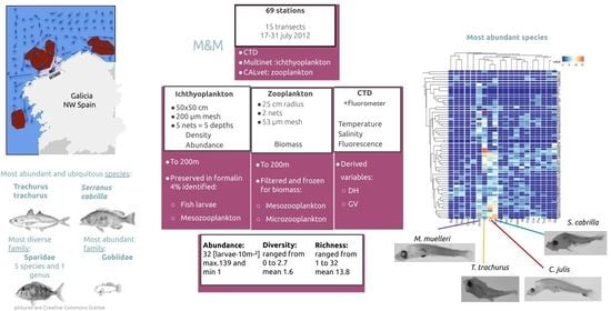
2. Materials and Methods

The CRAMER1207 survey was conducted aboard the Spanish research vessel Cornide de Saavedra along the Galician coast from 17 to 31 July 2012. Ninety-two stations were established in a sampling grid with the stations being distributed along fifteen transects perpendicular to the coastline and separated by eight nautical miles (nm), with a distance between stations of four nm (Figure 1). The transects extended from the 50 m isobath to the 500 m isobath, although due to weather conditions several stations were not sampled. Sampling elapsed for 7 days around the clock, from south to north. Temperature, salinity, and fluorescence were measured at every station with a conductivity–temperature–depth sensor (CTD, SBE25, Seabird Electronics, Inc., Bellevue, WA, USA), coupled to a Turner fluorometer. CTD’s casts and net hauls were performed at depths of 200 m at deeper stations or 5–10 m above the bottom at shallower stations.
Ichthyoplankton sampling was performed with a MultiNet (Midi, 0.50 m2 mouth opening) consisting of 5 nets of 200 μm mesh. The MultiNet was equipped with a Scanmar depth sensor as well as an electronic flowmeter located at the mouth. The depth strata, defined by the different depths at which each net was open, were 0–20 m, 21–40 m, 41–60 m, 61–100 m, and 100–200 m. At the stations located in depths shallower than 200 m the programmed terminal depth was adjusted and/or the number of strata reduced. The net was towed obliquely at 2 knots. The duration of the hauls was approximately one hour, and the mean volume filtered for each depth stratum was 25 L for the first three strata, 57 L for the fourth stratum, and 87 L for those at depths deeper than 100 m. Samples were preserved in a 4% seawater/formalin buffered solution with borax.
In the laboratory, all fish larvae were sorted and identified to the lowest possible taxonomic level. When identification at the species level was impossible, individuals were identified to the family level. Selected taxa (those with ≥20 larvae caught, both day and night) were photographed and, when possible, measured for standard length (±0.01 mm) using ImageJ (v. 1.53a).
Zooplankton was also sampled at each station from 200 m depth through vertical hauls using a CalVET net (25 cm diameter, 53 µm mesh size) equipped with an electronic flowmeter at its mouth. At shallower stations, hauling started 10 m above the bottom. Samples were filtered upon collection through 55 and 200 µ mesh sieves to separate micro (55–200 µm) and mesozooplankton (>200 µm). Both fractions were frozen in liquid nitrogen. In the lab, both fractions were dried in an oven at 60 °C to obtain an estimate of their weight [31]. Then, micro- and mesozooplankton weight were standardized with the total volume of filtered water to obtain biomass m−2. Mesozooplankton abundance (zooAbd) was calculated in the laboratory from the multinet samples for every depth stratum in each station by using a semi-automatic image analysis technique [32]. For that purpose, a subsample of 5 mL from each sample was stained with 0.1% eosin for 24 h and scanned; the resulting images were processed using Zoolmage and ImageJ software.

2.1. Environmental Data

Chlorophyll fluorescence, temperature, and salinity at 10 m depth (referred to as chlorophyll; Chlor, mg·m−3), sea surface temperature (SST, °C), and sea surface salinity (SSS, practical salinity scale) were extracted from the CTD data and used for most statistical analyses. Thermocline was obtained from the CTD data with the R packages oce and rLakeAnalyzer. The micro- and mesozooplankton biomass (MiB and MeB) values were referred as mg·m−2, mesozooplankton counts (Abdzoo) were standardized to ind·m−3, and depth stratum were also integrated for the sampled water column to obtain a value per station. Dynamic height (DH) was integrated over the water column and calculated from vertical profiles of temperature, salinity, and pressure using the 400 m depth as the reference level of no motion. At shallower stations, or when data were recorded only to 200 m, the density anomaly at the closest 400 m station was assigned to the deepest level sampled by the CTD. As DH and integrated water column density are inversely proportional [33], areas of high DH correspond to low salinity, warm seawater, and anticyclonic regions [34], whereas locations with low DH correspond to salty, cool seawater, and cyclonic eddy regions, showing gradients in frontal regions [35,36]. Geostrophic velocities (GVs) were obtained by the first derivative of the DH profiles analyzed on a regular grid of 3 × 3 nautical miles and extracting manually the closest value for each sampling point. Geostrophic velocities were used as an indicator of eddy boundaries and frontal regions because GVs should be higher in these regions [37,38]. Finally, spiciness was estimated, which is defined as a state variable and constructed to characterize water masses and indicate double-diffusive stability [39], being higher in warm and salty (spicy) waters [40]. Spiciness was calculated using R software v.3.5.1 [41] and the package oce [42].
We used published data on upwelling and wind regimes to understand the environmental scenario prevailing during the survey. The upwelling index and information about eddies was obtained from Instituto Español de Oceanografía [43]. Winds regime were obtained from the ‘Puertos del Estado’ database [44], specifically from the buoy located at Cabo Vilano (43.29° N and 9.12° W).
The maps of the physical and biological variables were constructed from the fitted variogram and posterior kriging of the values per station with the R packages gstat [45] and automap [46].

2.2. Community

Fish larval abundance was standardized to the number of larvae found beneath a 10 m2 area of sea surface [ind·10 m−2]. Similarly, larval densities were standardized to individuals 1000 m−3 and calculated using flowmeter measurements [47]. Larval fish diversity (Shannon–Wiener index) and species richness were calculated for each station. Densities were also calculated for each depth stratum.

2.3. Horizontal Distribution

Several regression models were tested to assess the influence of the biological and environmental variables (MiB, MeB, Chlor, zooAbd, depth, SSS, SST, DH, and GV) on the parameters of the LFC: larval abundance, diversity (Shannon index), and richness of species at every sampled station. These parameters were obtained integrating the number of larvae at every depth stratum in each sampling station.
Data exploration was carried out after testing for collinearity [48,49]. When the correlation between pairs of variables was >0.6, one of the variables was removed from analyses. Finally, the covariables included in the models were depth, SST, SSS, GV, Chlor, MeB, and MiB. Chlor and depth were log transformed to reduce the influence of extremely high values. The fish larval abundance was modeled using the general additive model (GAM), given the nonlinear behavior of some covariates in relation to the response variables. Richness and abundance were adjusted to a negative binomial distribution with a logistic link function, and diversity was adjusted to a normal distribution. To model larval abundance, we added the volume of water filtered at every station as an offset in the equation. The final model was selected following a forward stepwise procedure based on the AIC minimization. The model assumptions were verified by plotting the residuals against the fitted values, each covariate in the model, and each covariate not included in the model. The R package mgcv [50] was used to fit the model. The same procedure was used for the other LFC parameters.
Cluster and ordination methods were used to analyze the structure of the LFC using the matrix of the larval fish abundances, but selected taxa had to have abundances greater than 0.2 larvae·10 m−2 and be present at more than 5% of the stations, resulting in a matrix of twenty-one species. The abundance data were log (x + 1) transformed to dampen the influence of the most abundant species prior to obtaining the dissimilarity (Bray–Curtis) matrix [51,52]. R package NbClust [53] was used to find the more appropriated number of clusters, while ANOSIM (analysis of similarities) was performed to test the significance of the clusters. Hierarchical agglomerative clustering with average linking in conjunction with non-metric multidimensional ordination (nMDS) was used to identify assemblages.
The relationship between environmental factors and community structure was assessed with canonical correspondence analysis (CCA). The environmental data matrix included the values of the biological and oceanographic variables at a depth of 10 m. The selection of variables included in the CCA followed a forward stepwise procedure. Significance (p < 0.05) was tested with an ANOVA-like permutation test. Only those variables that significantly explained the species distribution pattern were included in the model. The canonical axes were also tested for significance with the same permutation test. All the ordinations were performed using the vegan package in R [54,55].
The relative length distribution of larvae was explored to assess the direction that the most influential currents were having in the LFC. Lengths were standardized to each species maximum length registered during the entire survey, as a proxy of age to infer the spawning area since smaller specimens will likely be nearer to the spawning area.

2.4. Vertical Distribution

A matrix with the densities of species with more than 20 individuals (adding the day and night collections) was created for the analysis of vertical and daily (day/night) distributions. This resulted in a matrix of fifteen species, five depth strata, and two light regimes. The depth strata were 0–20 m, 21–40 m, 41–60 m, 61–100 m, and >100 m. For the light regime analysis, the day period was defined as 7:30 am till 9:30 pm GMT, and the night period was defined as 10:30 pm till 6:30 am GMT, considering the sunrise and sunset time in the study area during sampling. Samples between 6:30–7:30 am and 9:30–10:30 pm were considered as transitional and discarded for this analysis. The weighted mean depths (WMDs) of the larvae in each (MultiNet) haul were calculated as the center of masses of the larval distribution:
WMD = i = 1 5 n i × d i n i
where ni is the density of fish larvae [ind·1000 m3] in the ith stratum, and di is the mid-depth of the ith stratum [56].
The amplitude of the diel vertical migrations (DVM) was calculated as the difference between the average WMDs for the day and night periods (DVM= WMDday − WMDnight). Positive values of DVM (type I) correspond to species that move towards the surface during the night, whereas negative values indicate downward movement at night (type II) [57]. A T-test was used to test for the significance of the DVM for each species.
The larval densities were used to calculate the Bray–Curtis matrix of distances from the log x + 1-transformed data, these distances were used for the clustering and nMDS. ANOSIM was performed to test if the vertical structure of larval assemblages existed depending on depth and time of day.
Differences between depth strata and day/night abundances were tested using the permutational multivariate analysis of variance using distance matrices (PERMANOVA) with the R package vegan.
Because DVM is often a size-related (ontogenetic) phenomenon, with larvae starting to migrate after yolk sac absorption [57], differences in larval length between day and night and depth strata were also assessed for the selected taxa by using a two-factor ANOVA. When significant differences were found, the Tukey post hoc test was conducted to identify which groups were significantly different from the other. The ANOSIM, NMDS, and distance matrix calculations were done using the R package vegan.
The standard deviation and standard error were used to describe the dispersion of environmental and biological data.

3. Results

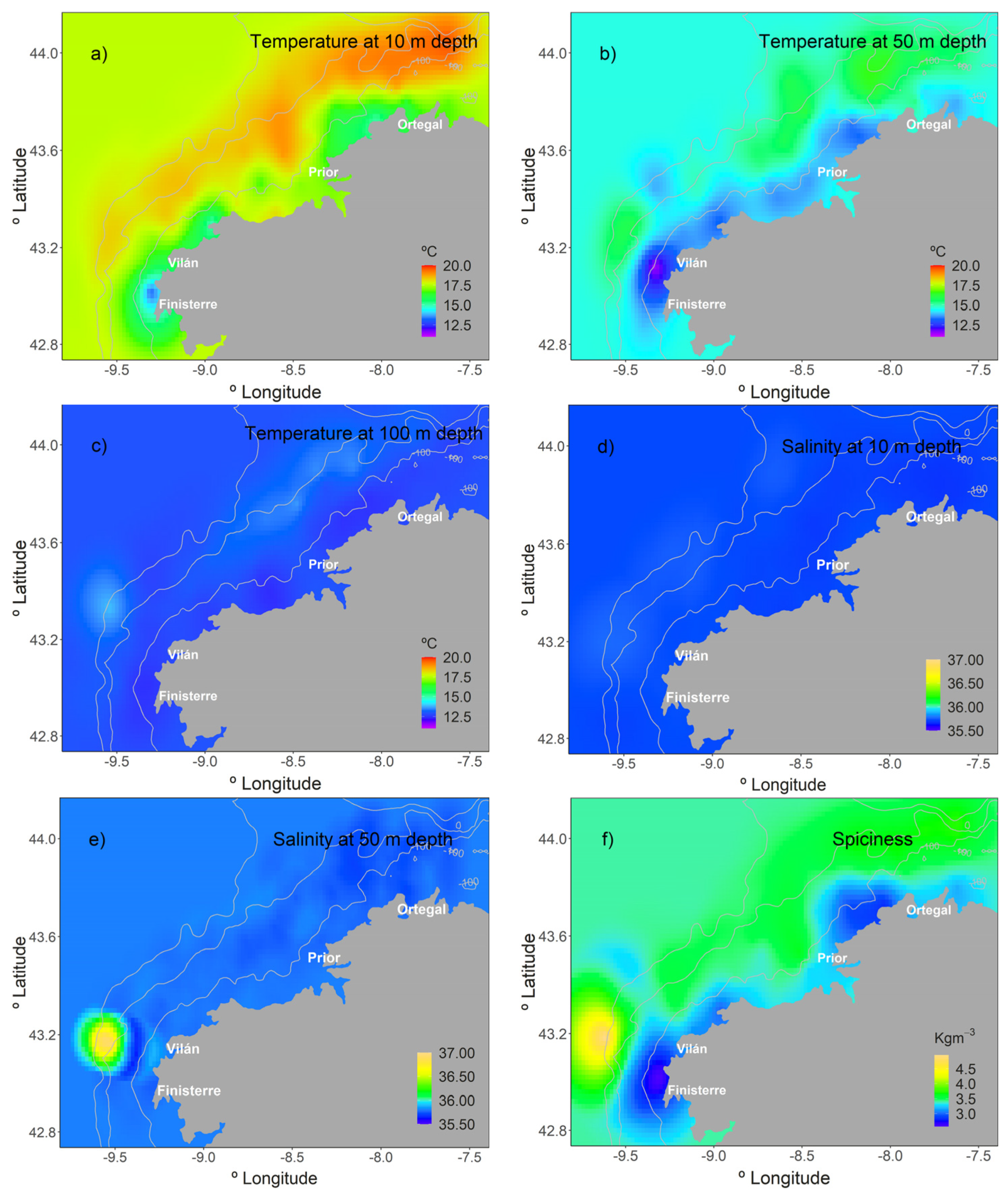
3.1. Environmental Variables

There was a north-prevailing wind regime during the sampling period, increasing its intensity towards the end of the cruise, although in the preceding days of the survey, northerly and southerly pulses were alternating. The change of wind direction resulted in an average upwelling index (UI) for the month of July below the historical average value for this period (21 m3·s−1·km−1 and 370 m3·s−1·km−1, respectively). However, the dominant upwelling conditions prevailed during the cruise and during the four previous days—the mean UI was 191 m3. s−1.km−1.
The hydrographic structure along the sampled area changed due to the wind regime and coastal orientation. Upwelling events occurred south and north of the grid area during the survey, although they were slightly weaker in the north. In the Artabro Gulf area, the average temperatures were higher than those in the surroundings and linked to the higher GV, which suggests the presence of an anticyclonic eddy. Nevertheless, the upwelling event was not strong enough to completely break the stratification (except partially in the inner shelf), as the water column was stratified in the upper ~60 m, according to CTD’s profiles, except when the wind-driven mixed layer reached the top 30 m.
The SST showed an along-shelf temperature front with colder waters occupying the inner shelf; it varied between 13.2 °C next to Cape Finisterre and 19.5 °C west of Cape Ortegal (Figure 2a). The lowest SSS (35.6) were associated with freshwater masses from river runoff near Cape Ortegal, although other coastal low values were found south of Artabro Gulf (35.7). The maximum SSS (35.8) was recorded near the Cape Finisterre over the 200 m isobath (Figure 2d). Temperature and salinity at different depths show cross-shelf gradients. Temperature gradient was from minimum to maximum, from coast, outwards. It ranged from 12.5 °C to 17.8 °C (between bathymetric 10 m and 150 m) and reached its minimum north of Finisterre cape and maximum in the north of the area, over the 200–500 bottom isobaths (Figure 2a,b). Salinity had minute variations with depth, except off Finisterre cape where salinity reached 36.9 at 50 m depth, over the 200–500 isobath (Figure 2e).
A front separates the colder and fresher waters of the inner shelf from the warmer and saltier offshore waters. This front is well reflected by the spiciness, which ranged from 2.3 to a maximum of 5.5 kg.m−3 offshore of Cape Finisterre, that reveals the presence of a subsurface thermohaline front (Figure 2f).
The gradient between the cold freshwater and warm salty water resulted in an area of low dynamic heights along the inner shelf (over grounds <100 m) and a geostrophic current flowing southwestward along the 100 m isobath. The dynamic height ranged from −3.1 to 3.4 cm in the whole area, and geostrophic velocities were weak (<10 cm·s−1 in the upper levels and <5 cm·s−1 at depths under 100 m) but exceeded 30 cm·s−1 at some points near Cape Ortegal (Figure 1). The general currents in the area informed of an anticyclonic mesoscale feature associated with high temperature and salinity, stacking in the gulf during the entire period.

3.2. Biological Variables

Regarding the biological variables, the average superficial chlorophyll fluorescence was 8.4 ± 7.7 mg·m−3, microzooplankton biomass was 1033.1 ± 220.4 mg·m−2, mesozooplankton biomass was 2661.5 ± 916.2 mg·m−2, and mesozooplankton abundance was 3320.4 ± 1472 ind·m−3. Primary production (Chlor) at 10 m depth was higher near the coast than in the shelf break. The mean Chlor at the stations below the 100 m isobath was 12.3 ± 9.5 mg·m−3 and 5.8.1 ± 4.8 mg·m−3 in stations between 100 and 200 m isobaths (Figure 3a). The MiB maximum (1836.3 mg·m−2) was located below the 100 m isobaths off the Finisterre coast and in a small area of the Artabro coast (Figure 3b), while the MeB maximum (4990.5 mg·m−2) was observed between the 100–200 m isobaths in the Finisterre area and over the 200 m isobath in front of the Artabro coast (Figure 3c). Zooplankton abundance showed its maximum (7405.2 ind·m−3) between 200 and 500 isobaths north of Finisterre cape and in some stations in the Artabro Gulf (6945.1 ind·m−3). Concerning the vertical distribution of chorophyll, the maximum was concentrated in the 20–60 m layer (74.1–0.6 mg·m−3, max-min), while the maximum zooplankton abundance was mainly in the 0–60 m layer (3635.9–101.2 ind·m−3, max-min).

3.3. Descriptors and Structure of the Larval Fish Community

A total of 2189 larvae belonging to 64 taxa and grouped into 31 families were collected and identified (Table 1). The percentage of unidentified larvae (2.4%) was due to a lack of early life history descriptions of the regional species, damaged specimens, and to a major extent due to the early development stage of the larvae and lack of characteristic features. The abundance per station ranged from 5.7 to 749.6 larvae·10 m−2, and averaged 217.2 ± 189.1 larvae·10 m−2, with a maximum of 139 larvae collected in one sampling station (Figure 4a). The most diverse family represented was Sparidae, with six species (one identified to the genus level), and Gobiidae was the most abundant (specimens were grouped into the family level due to the high difficulty in their classification). Two coastal species, Trachurus trachurus (pelagic) and Serranus cabrilla (demersal), were the most abundant and ubiquitous species, and the unique mesopelagic (oceanic slope) species that was among those with relative abundance higher than 1% was Maurolicus muelleri (Table 1).
The maximum abundance (749.6 larvae·10 m−2) of larvae was recorded on the Artabro coast and it was mainly due to the contribution of the family Gobiidae (161.8 larvae·10 m−2) and non-identified larvae (275 larvae·10 m−2). The second highest value of abundance (668.3 larvae·10 m−2) was found south of Artabro Gulf, where T. trachurus contributed the most to the total larvae abundance (244 larvae·10 m−2) (Figure 4a). Regarding diversity of the community, the highest value was recorded between Cape Prior and Cape Ortegal and for richness the maximum was registered near the Artabro coast (Figure 4b,c). The species richness values ranged from 0 to 20 (11.9 ± 4.7), and the Shannon index ranged from 0 to 2.7 (1.9 ± 0.5).
The mean standard length of T. trachurus was 3 ± 1.3 mm, ranging from 1.1 to 7.0 mm; for S. cabrilla it was 3.7 ± 1.2 mm, ranging from 1.4 to 6.8 mm; for M. muelleri it was 7 ± 2.1 mm, ranging from 1.6 to 11.2 mm; for C. julis it was 3.2 ± 1.3 mm, ranging from 1.2 to 10.7 mm.
The species that define the summer LFC did not show any horizontal structure (Figure 5); they were not differentially grouped, even among coastal-, shelf-, or slope-spawning species as indicated by cluster analysis. The method used to find the best grouping for the dissimilarity matrix identified two clusters as the best result for the matrix of dissimilarities (Figure 5a,c), which was corroborated by the nMDS ordination (Figure 5b). Groups separated at a similarity level of 85%. ANOSIM was performed as well and confirmed this grouping (R statistic = 0.8, p < 0.005). ANOSIM was also used to test the three clusters option, but results were not supported (R statistic = 0.3, p < 0.005).
In general, no differential pattern was evident when mapping the most abundant taxa, except for S. pilchardus (Figure 6b) and E. encrasicolus (Figure 6e), which were concentrated in shallow waters and almost entirely near to Cape Ortegal, respectively. Serranus cabrilla was widespread over the study area but dominating north of Artabro Gulf (Figure 6c), while M. muelleri had no clear distribution pattern (Figure 6f). Trachurus trachurus and C. julis were more abundant in the Artabro Gulf, although C. julis showed a more northward distribution (Figure 6a).
From the ontogenic point of view, the horizontal distribution of the larvae of the most abundant species did not show any trend, except for S. pilchardus which appears to be concentrated by the coast (Figure 6b). Overall, the horizontal distribution of larvae according to relative length showed that smaller larvae accumulated in the northern area, from the Artabro Coast to Cape Ortegal, while bigger larvae were distributed between Cape Vilán and Cape Ortegal and towards the slope (Figure 7).
In contrast, according to the multinet samples results, the vertical distribution of larvae appeared well structured, showing higher abundances in the first 40 m. The PERMANOVA analysis (R2 = 0.27, p ≤ 0.001) and Tukey post hoc confirm these differences (Table 2). Mesozooplankton abundance was higher in the first 60 m (min-max, mean: 101.2–3635.9, 988.7 ind·m−3), both day (101.2–3635.9, 913.3 ind·m−3) and night (155.0–3566.1, 1056.8 ind·m−3) (Table 3). Most of the species were almost absent from the 60–200 m depth stratum (except some myctophids) during the day and night. The vertical distribution of the most abundant species was not significantly correlated with mesozooplankton, except for A. thori and S. pilchardus (Table 4). For their distribution in the water column, cluster and ordination analyses (Figure 5d,e) showed four groups (ANOSIM R statistic = 0.95, p < 0.005) of larvae at a similarity level of 40% (Figure 5d,e). The resulting groups are as follows: (1) S. porcus and T. mediterraneus; (2) M. punctatum, B. glaciale, and M. merluccius; (3) M. muelleri, C. julis, S. cabrilla, Callionymidae, and T. trachurus; and (4) C. maderensis, C. rupestris, C. macrophtalma, P. acarne, P. pilicornis, E. encrasicolus, A. thori, S. pilchardus, C. aper, and T. draco. However, the ANOSIM detected only a slight segregation along the water column (ANOSIM R statistic = 0.3, p > 0.005), and no differences in community composition between day and night (R statistic = 0.06 p < 0.005). No significant correlation between the vertical migrations of the pool of fish larvae and the mesozooplankton was observed, except for M. muelleri, C. julis, and S. cabrilla that performed significant type I DVMs (i.e., upward movement at night) (Table 5). The mean vertical displacement was 7.8 ± 6.5 m for the selected species, with M. muelleri being the species that had a wider migration (27 m).
Regarding the analysis of length distributions by depth (Figure 8) and day/night period, the results of the two-factor ANOVA showed significant differences in day/night larval length for only two species. In the case of M. Muelleri, larvae caught at night were significantly larger than larvae caught during the daytime, while the inverse pattern was observed for S. cabrilla. Differences in larval length in relation to depth were significant for five taxa; C. julis, M. muelleri, S. pilchardus, and T. trachurus were larger at deeper strata, while the opposite trend was observed for L. crocodilus. The interaction between daytime and depth was significant only for T. trachurus (Table 6).

3.4. Relationship between the LFC and Environmental Variables

The regression models constructed to explain the variation in the abundance, diversity, and richness of the fish larvae community in relation to the biotic and abiotic variables explained 66.1%, 59%, and 51.5% of the variability, respectively. In the case of fish larvae abundance, depth, abundance of zooplankton, and GV were the most important drivers followed by SST. For diversity, SSS and GV were the most relevant drivers followed by SST. For richness, only SSS and GV had a significantly influence in setting its variability (Table 7). In general, fish larvae abundance, diversity, and richness increase with increasing temperature, salinity, and geostrophic velocities, while zooplankton abundance has a positive relationship with fish larvae abundance, despite decreasing with depth.
From a multivariate perspective, the CCA resulted in a simplified model (significant p < 0.01) that included three environmental variables: GV, SST, zooplankton abundance (Figure 9). However, the proportion of total variance explained by the environmental constraints was only 18% from which the first two constrained axis explained 11%, and 7%, respectively. Among the species more influenced by temperature were some oceanic myctophids (B. glaciale, M. punctatum, C. maderensis), while the abundance of coastal species, such as S. pilchardus (Figure 6b), was more influenced by higher values of chlorophyll. However, in general, there was no clear pattern or evident association between species and environmental conditions, and none of the variables showed great influence on the species distribution, as reflected by the small percentage of variation explained by the constrains.

4. Discussion

4.1. Environmental Conditions and Their Influence on the Summer LFC

The abiotic conditions in the Artabro Gulf pointed that this zone was a transition area between two water masses during the summer of 2012, as indicated by the sea surface temperature and salinity and of spiciness which showed a subsurface front off Cape Finisterre. In front of Finisterre cape there was a point which can be reflecting the emergence of water from the subtropical ENACW (Figure 2f), defined as a spicy water [4,15,53].
The upwelling conditions were fully established during the sampling period (predominant northern winds), despite that northerly and southerly wind pulses were alternating in the weeks preceding the survey. Usually, the response time between wind conditions and oceanographic changes in the Galician coast is of 3 days [58]. The water column, which had conditions consistent with summer stratification in temperate regions [59], had a mixed layer of variable depth that was narrower in the Artabro Gulf area. Additionally, an anticyclonic eddy in front of the Gulf was constant during the cruise as indicated by the higher geostrophic velocities along the northwestern coast and in a southward surface flow that moved parallel to the coast and changing direction with coastal orientation (Figure 1). Both CCA and GAMs elucidated the influence of the environment in the structure and descriptors of the LFC, pointing to the upwelling and currents as the main forces conforming the summer community. In both analyses, zooplankton abundance showed a positive relationship with the larvae abundance and the LFC species distribution.
Primary production was higher along the coast than offshore, especially along the Artabro coast next to Ortegal, where the highest superficial chlorophyll concentrations reached 40 mg·m−3. Regarding secondary production, Fletcher [60] analyzed the egg distribution in the same area and period, and marked the cape next to Ortegal (Estaca de Bares) as the point with the highest egg abundance and Finisterre cape as the point with the lowest egg abundance. These results coincided with the larval distribution seen in this work. An analysis of the LFC in a different environmental regime (spring) also found the same areas to have the highest abundances of eggs and larvae [22], coincident with a cross-shelf frontal region.
This studies about egg distribution plus the distribution of larvae by relative length, point to the Artabro coastal area as a spawning ground for many of the species detected in the present study. This distribution highlights the existence of a current that transports fish eggs southwards from the northern spawning area, and following the clockwise direction of the eddy and the offshore superficial current of the upwelling, which was stronger in the south. Young larvae were gathered by the currents and transported southwestwards with the surface current as they developed. The Artabro coast coincides with the change in orientation of the Galician coast (north to northwest), which makes it more sensitive to northern winds and hence more prone to upwelling events in summer. The presence of a single larval fish assemblage was already seen in spring and then was attributed to offshore Ekman transport associated with a coastal upwelling event, which homogenized the LFC in the cross-shelf direction [22].
For the upwelling areas, the vertical position of fish larvae throughout the day and night also determines if they are retained in shallow and productive waters or advected offshore [61]. Larvae with near-surface distributions are more susceptible to offshore transport associated with coastal upwelling than larvae with deeper distributions, which are moved shoreward [61]. Thus, larval transport across the shelf depends on the horizontal location of the spawning ground and vertical position at which eggs were spawned. The vertical summer distribution of the LFC in the surface layer suggests that most taxa with neritic spawning (e.g., S. pilchardus, E. encrasicolus, T. trachurus) should spread over the shelf, and oceanic larvae (Sternoptychidae: M. muelleri, Mychtophidae: M. punctatum), which spawn at greater depths, should be driven shoreward by the cold bottom flow [24]. It was been noted that the highest densities of eggs were above the mixed layer [60]. Eggs from neritic species (S. pilchardus, E. encrasicolus, T. trachurus) were found in higher abundancies at depths lower than 50 m, while eggs from mesopelagic species, such as M. muelleri, were found at depths between 50 and 150 m on the Artabro coast [60]. The horizontal distribution of the most abundant species seems to indicate that larvae were transported passively southwards from a spawning area along the northwestern coast.
Regarding the cross-shelf distribution, the abundance of neritic species (Gobiidae, Blenidae, Cupleidae) decreased from the coast to the 200 m isobaths, while oceanic species had the opposite distribution. It had been reported that the spatial distribution of larvae could be quite heterogeneous in coastal areas with a highly variable shelf structure, and that the existence of a shelf slope front associated with a current flow parallel to the coast would contribute to larval concentrations of mesopelagic and shelf species over the shelf break [62], as we observed in this study. Thus, the front detected in the Galician shelf in the summer of 2012 could act as a barrier preventing offshore dispersion. The importance of frontal regions for fish spawning and the concentration of fish larvae has already been documented [30,63]. Settlement and recruitment of the coastal species will be favored by retention structures; here lies the importance of the knowledge of seasonal environmental conditions to understand the mechanisms that affect fish larval stages.

4.2. Seasonal LFC in Galician Waters

The LFC was highly diverse and rich, with lower abundances than in winter or spring and without dominant species [23,24]. The LFC was made up of a mixture of coastal, neritic, and oceanic mesopelagic species, which coincides to a great extent with the composition and diversity of coastal and transitional assemblages found in the central Cantabrian Sea in summer [52]. The Galician summer assemblage seems to differ from the spring assemblage. Diversity was slightly higher in the summer of 2012 compared with spring (summer: 0–2.7, mean 1.9, spring: 0–3.1, mean 1.8) but richness lightly lower (summer: 0–20, mean 11.9, spring: 1–32, mean 13.8), and abundance considerably lower (summer: 5.7–749.6, mean 217.2 larvae·10 m−2, spring: 4.6–26147.3, mean of 939.8 larvae 10m−2) [25]. However, due to the markedly different seasonal environmental conditions and the impact that it has on communities and poor knowledge about its dynamics, it is impossible to evaluate if such differences or similarities are permanent or due to specific seasonal fluctuations or to species protracted reproductive period or adaptions.
In the literature, there are some descriptions about the spawning season for some of the dominant species. The spawning period of T. trachurus begins in March–April and ends November [64], while for S. cabrilla it begins in February and ends in July in southern latitudes [65]. Regarding E. encrasicolus, its spawning season increases with decreasing latitude from Bay of Biscay to Gulf of Cádiz in April–August to April–November [66]. Sardina pilchardus has the main spawning period during October–June, peaking in December–March, but with longer duration and earlier peak at lower latitudes [67]. Unfortunately, there are no reproductive studies for most species—including C. julis, P. acarne, P. pilicornis, and T. draco in the Galician waters. Regarding the alongshore composition, there are different structures of the LFC between the northern and northwestern coasts of Galicia in the spring of 2012 [23], which were not evident in the summer. Yet, more data should be collected to obtain more robust conclusions.

5. Conclusions

The larval fish community of the Galician coast seems to be shaped by the interaction between fish spawning location, concurrence of two water masses, coastal upwelling, and an anticyclonic eddy. This interaction resulted in a lack of structure in the across and along the shelf. The eddy circulation may have transported fish eggs and larvae from a spawning area in the north, which with the help of winds (and consequent upwelling) pushed larvae southwards and offshore while avoiding oceanic dispersion. This scenario kept the larvae retained in the same area, either if they were spawned by shelf-, coastal-, or slope-spawning species. Similarly, changes in the seasonal environmental conditions could result in major changes affecting interspecific competition and reproductive success, which finally would be reflected in recruitment and stock abundance.

Author Contributions

Conceptualization, formal analysis, and methodology, S.R.U.; investigation, F.S.-R., A.R.V.C. and S.R.U.; resources, F.S.-R.; writing—original draft preparation, S.R.U.; writing—review and editing, R.D.-P. and F.S.-R.; supervision, F.S.-R.; project administration, F.S.-R.; funding acquisition, F.S.-R. All authors have read and agreed to the published version of the manuscript.

Funding

This work was funded by the Spanish research project CRAMER (CTM2010-21856-CO3-02), the Galician research project ECOPREGA (10MMA602021PR), and the “Mobility grant (Research, innovation and growth plan 2011-2015, I2C) from the Innovation agency of the Xunta de Galicia. File 20/2014”.

Institutional Review Board Statement

Ethical review and approval were waived for this study, because the described scientific sampling did not require ethical permission according to the applicable international, EU and national laws.

Informed Consent Statement

Not applicable.

Data Availability Statement

The data presented in this study are available on request from the corresponding author.

Acknowledgments

We greatly appreciate the assistance of the crew of the RV ‘Cornide de Saavedra’, all the participants of the ‘Cramer 1207’ cruise, and J.M. Rodriguez from the Instituto Español de Oceanografia (IEO Gijón) for his valuable help with larval identification. Águeda Cabrero (IEO Vigo) provided DH and GV data, Raúl Laiz (IEO Málaga) provided biomass data and César Fletcher (AZTI) provided zooplankton abundance. Special thanks to the reviewers and Academic Editor for their precise and insightful comments, and valuable contributions to this manuscript.

Conflicts of Interest

The authors declare no conflict of interest. The funders had no role in the design of the study; in the collection, analyses, or interpretation of data; in the writing of the manuscript; or in the decision to publish the results.

References

  1. Cowen, R.K.; Sponaugle, S. Larval Dispersal and Marine Population Connectivity. Annu. Rev. Mar. Sci. 2009, 1, 443–466. [Google Scholar] [CrossRef] [PubMed] [Green Version]
  2. Torres, R.; Barton, E.D.; Miller, P.; Fanjul, E. Spatial patterns of wind and sea surface temperature in the Galician upwelling region. J. Geophys. Res. Space Phys. 2003, 108, 1–14. [Google Scholar] [CrossRef] [Green Version]
  3. Fraga, F. Upwelling off the Galician Coast, Northwest Spain. In Coastal Upwelling; Richards, F.A., Ed.; American Geophysical Union (AGU): Washington, WA, USA, 1981; pp. 176–182. [Google Scholar]
  4. González-Nuevo, G.; Nogueira, E. Intrusions of warm and salty waters onto the NW and N Iberian shelf in early spring and its relationship to climate variability. J. Atmos. Ocean Sci. 2005, 10, 361–375. [Google Scholar] [CrossRef]
  5. Alvarez-Salgado, X.A.; Figueiras, F.G.; Perez, F.F.; Groom, S.; Nogueira, E.; Borges, A.V.; Chou, L.; Castro, C.G.; Moncoiffé, G.; Ríos, A.; et al. The Portugal coastal counter current off NW Spain: New insights on its biogeochemical variability. Prog. Oceanogr. 2003, 56, 281–321. [Google Scholar] [CrossRef] [Green Version]
  6. Ríos, A.F.; Pérez, F.F.; Fraga, F. Water masses in the upper and middle North Atlantic Ocean east of the Azores. Deep Sea Res. Part A Oceanogr. Res. Pap. 1992, 39, 645–658. [Google Scholar] [CrossRef] [Green Version]
  7. Haynes, R.; Barton, E.D. A poleward flow along the Atlantic coast of the Iberian peninsula. J. Geophys. Res. Space Phys. 1990, 95, 11425–11441. [Google Scholar] [CrossRef] [Green Version]
  8. Álvarez, I.; Prego, R.; de Castro, M.; Varela, M. Galicia upwelling revisited: Out-of-season events in the rias (1967–2009)|Revisión de los eventos de afloramiento en Galicia: Eventos fuera de temporada en las rías (1967–2009). Ciencias Mar. 2012, 38, 143–159. [Google Scholar] [CrossRef] [Green Version]
  9. Casabella, N.; Lorenzo, M.; Taboada, J. Trends of the Galician upwelling in the context of climate change. J. Sea Res. 2014, 93, 23–27. [Google Scholar] [CrossRef]
  10. Prego, R.; Bao, R. Upwelling influence on the Galician coast: Silicate in shelf water and underlying surface sediments. Cont. Shelf Res. 1997, 17, 307–318. [Google Scholar] [CrossRef] [Green Version]
  11. Somoza, L.; Medialdea, T.; González, J.; León, R.; Palomino, D.; Rengel, J.; Fernández-Salas, L.M.; Vazquez, J.-T. Morphostructure of the Galicia continental margin and adjacent deep ocean floor: From hyperextended rifted to convergent margin styles. Mar. Geol. 2018, 407, 299–315. [Google Scholar] [CrossRef]
  12. Bode, A.; Alvarez-Ossorio, M.; Cabanas, J.; Miranda, A.; Varela, M. Recent trends in plankton and upwelling intensity off Galicia (NW Spain). Prog. Oceanogr. 2009, 83, 342–350. [Google Scholar] [CrossRef]
  13. Álvarez-Salgado, X.A.; Labarta, U.; Fernández-Reiriz, M.J.; Figueiras, F.G.; Rosón, G.; Piedracoba, S.; Filgueira, R.; Cabanas, J.M. Renewal time and the impact of harmful algal blooms on the extensive mussel raft culture of the Iberian coastal upwelling system (NE Europe). Harmful Algae 2008, 7, 849–855. [Google Scholar]
  14. Ruiz-Villarreal, M.; Álvarez-Salgado, X.A.; Cabanas, J.M.; Pérez, F.F.; Castro, C.G.; Herrera, J.L.; Piedracoba, S.; Rosón, G. Variabilidade climática e tendencias decadáis nos forzamentos meterorolóxicos e as propiedades das augas adxacentes a Galicia. In Evidencias e Impactos do Cambio Climáticoen Galicia; de Medio Ambiente, C., Ed.; Xunta de Galicia: Galicia, Spain, 2009; pp. 271–286. [Google Scholar]
  15. Tenore, K.R.; Alonso-Noval, M.; Alvarez-Ossorio, M.; Atkinson, L.P.; Cabanas, J.M.; Cal, R.M.; Campos, H.J.; Castillejo, F.; Chesney, E.J.; Gonzalez, N.; et al. Fisheries and oceanography off Galicia, NW Spain: Mesoscale spatial and temporal changes in physical processes and resultant patterns of biological productivity. J. Geophys. Res. Space Phys. 1995, 100, 10943–10966. [Google Scholar] [CrossRef]
  16. Fariña, A.; Freire, J.; González-Gurriarán, E. Demersal Fish Assemblages in the Galician Continental Shelf and Upper Slope (NW Spain): Spatial Structure and Long-term Changes. Estuar. Coast. Shelf Sci. 1997, 44, 435–454. [Google Scholar] [CrossRef]
  17. Santos, M.B.; González-Quirós, R.; Riveiro, I.; Iglesias, M.; Louzao, M.; Pierce, G.J. Characterization of the pelagic fish community of the north-western and northern Spanish shelf watersa. J. Fish Biol. 2013, 83, 716–738. [Google Scholar] [CrossRef]
  18. Ferreiro, M.; Labarta, U. Distribution and abundance of teleostean eggs and larvae on the NW coast of Spain. Mar. Ecol. Prog. Ser. 1988, 43, 189–199. [Google Scholar] [CrossRef]
  19. Rodríguez, J. Temporal and cross-shelf distribution of ichthyoplankton in the central Cantabrian Sea. Estuar. Coast. Shelf Sci. 2008, 79, 496–506. [Google Scholar] [CrossRef]
  20. Azeiteiro, U.M.; Bacelar-Nicolau, L.; Resende, P.; Gonçalves, F.J.M.; Pereira, M.J. Larval fish distribution in shallow coastal waters off North Western Iberia (NE Atlantic). Estuar. Coast. Shelf Sci. 2006, 69, 554–566. [Google Scholar] [CrossRef] [Green Version]
  21. Rodriguez, J.M.; Gonzalez-Pola, C.; Lopez-Urrutia, A.; Nogueira, E. Composition and daytime vertical distribution of the ichthyoplankton assemblage in the central cantabrian Sea shelf, during summer: An eulerian study. Cont. Shelf Res. 2011, 31, 1462–1473. [Google Scholar] [CrossRef]
  22. Rodriguez, J.; González-Nuevo, G.; Gonzalez-Pola, C.; Cabal, J. The ichthyoplankton assemblage and the environmental variables off the NW and N Iberian Peninsula coasts, in early spring. Cont. Shelf Res. 2009, 29, 1145–1156. [Google Scholar] [CrossRef]
  23. Rodriguez, J.M. Assemblage structure of ichthyoplankton in the NE Atlantic in spring under contrasting hydrographic conditions. Sci. Rep. 2019, 9, 8636. [Google Scholar] [CrossRef] [Green Version]
  24. Rodríguez, J.M.; Cabrero, A.; Gago, J.; Guevara-Fletcher, C.; Herrero, M.; Hernandez de Rojas, A.; García-García, A.; Laiz-Carrión, R.; Vergara, A.; Alvarez, P.L.; et al. Vertical distribution and migration of fish larvae in the NW Iberian upwelling system during the winter mixing period: Implications for cross-shelf distribution. Fish. Oceanogr. 2015, 24, 274–290. [Google Scholar] [CrossRef]
  25. Rodriguez, J.M.; Cabrero, A.; Gago, J.; Garcia, A.; Laiz-Carrion, R.; Piñeiro, C.; Saborido-Rey, F. Composition and structure of fish larvae community in the NW Iberian upwelling system during the winter mixing period. Mar. Ecol. Prog. Ser. 2015, 533, 245–260. [Google Scholar] [CrossRef] [Green Version]
  26. García-Seoane, E.; Álvarez-Colombo, G.; Miquel, J.; Rodríguez, J.; Fletcher, C.G.; Álvarez, P.; Saborido-Rey, F. Acoustic detection of larval fish aggregations in Galician waters (NW Spain). Mar. Ecol. Prog. Ser. 2016, 551, 31–44. [Google Scholar] [CrossRef] [Green Version]
  27. Cowan, J.H., Jr.; Rice, J.C.; Walters, C.J.; Hilborn, R.; Essington, T.E.; Day, J.W., Jr.; Boswell, K.M. Challenges for Implementing an Ecosystem Approach to Fisheries Management. Mar. Coast. Fish. 2012, 4, 496–510. [Google Scholar] [CrossRef]
  28. Frank, K.T.; Leggett, W.C. Fisheries Ecology in the Context of Ecological and Evolutionary Theory. Annu. Rev. Ecol. Syst. 1994, 25, 401–422. [Google Scholar] [CrossRef]
  29. Browman, H.I.; Stergiou, K.I. Perspectives on ecosystem-based approaches to the management of marine resources. Mar. Ecol. Prog. Ser. 2004, 274, 269–270. [Google Scholar] [CrossRef] [Green Version]
  30. Govoni, J.J. Fisheries oceanography and the ecology of early life histories of fishes: A perspective over fifty years. Sci. Mar. 2005, 69, 125–137. [Google Scholar] [CrossRef]
  31. Lovegrove, T. The Determination of the Dry Weight of Plankton and the Effect of Various Factors on the Values Obtained; Allen and Unwin: St. Leonards, NSW, Australia, 1966. [Google Scholar]
  32. Bachiller, E.; Fernandes, J.A. Zooplankton Image Analysis Manual: Automated identification by means of scanner and digital camera as imaging devices. Rev. Investig. Mar. 2011, 18, 16–37. [Google Scholar]
  33. Pond, S.; Pickard, G.L. Introductory Dynamical Oceanography, 2nd ed.; Butterworth-Heinemann: Oxford, UK, 1983. [Google Scholar]
  34. Asch, R.G.; Checkley, D.M. Dynamic height: A key variable for identifying the spawning habitat of small pelagic fishes. Deep. Sea Res. Part I Oceanogr. Res. Pap. 2012, 71, 79–91. [Google Scholar] [CrossRef]
  35. Siegel, D.A.; McGillicuddy, D.; Fields, E.A. Mesoscale eddies, satellite altimetry, and new production in the Sargasso Sea. J. Geophys. Res. Space Phys. 1999, 104, 13359–13379. [Google Scholar] [CrossRef] [Green Version]
  36. Lindo-Atichati, D.; Bringas, F.; Goni, G.; Mühling, B.; Muller-Karger, F.; Habtes, S. Varying mesoscale structures influence larval fish distribution in the northern Gulf of Mexico. Mar. Ecol. Prog. Ser. 2012, 463, 245–257. [Google Scholar] [CrossRef] [Green Version]
  37. Peliz, A.; Rosa, T.L.; Santos, A.M.P.; Pissarra, J.L. Fronts, jets, and counter-flows in the Western Iberian upwelling system. J. Mar. Syst. 2002, 35, 61–77. [Google Scholar] [CrossRef]
  38. Rhines, P.B. Mesoscale Eddies, 3rd ed.; Elsevier Inc.: Amsterdam, The Netherlands, 2008. [Google Scholar]
  39. Flament, P. Finestructure and Subduction Associated with Upwelling Filaments; University of California San Diego: La Jolla, CA, USA, 1986. [Google Scholar]
  40. Flament, P. A state variable for characterizing water masses and their diffusive stability: Spiciness. Prog. Oceanogr. 2002, 54, 493–501. [Google Scholar] [CrossRef]
  41. R Core Team. R: A Language and Environment for Statistical Computing; R Foundation for Statistical Computing: Vienna, Austria, 2020. [Google Scholar]
  42. Kelley, D.E. Oceanographic Analysis with R; Springer: New York, NY, USA, 2018. [Google Scholar]
  43. Instituto Español de Oceanografía. Data Viewer IEO. 2011. Available online: http://www.indicedeafloramiento.ieo.es/index1_en.php (accessed on 12 November 2018).
  44. Organismo Público Puertos del Estado, Ministerio de Transportes. Puertos del Estado—Oceanografía. Available online: http://www.puertos.es/es-es/oceanografia/ (accessed on 12 November 2018).
  45. Gräler, B.; Pebesma, E.; Heuvelink, G. Spatio-Temporal Interpolation using gstat. R J. 2016, 8, 204–218. [Google Scholar] [CrossRef]
  46. Hiemstra, P.H.; Pebesma, E.; Twenhöfel, C.J.; Heuvelink, G.B. Real-time automatic interpolation of ambient gamma dose rates from the Dutch radioactivity monitoring network. Comput. Geosci. 2009, 35, 1711–1721. [Google Scholar] [CrossRef]
  47. Smith, P.E.; Richardson, S.L. Standard techniques for pelagic, fish egg and larva surveys. FAO Fish. Tech. Pap. 1977, 175, 100. [Google Scholar]
  48. Zuur, A.F.; Ieno, E.N.; Walker, N.J.; Saveliev, A.A.; Smith, G.M. Mixed Effects Models and Extensions in Ecologywith R; Springer: New York, NY, USA, 2009. [Google Scholar]
  49. Zuur, A.F.; Ieno, E.N.; Elphick, C.S. A protocol for data exploration to avoid common statistical problems. Methods Ecol. Evol. 2009, 1, 3–14. [Google Scholar] [CrossRef]
  50. Wood, S.N. Fast stable restricted maximum likelihood and marginal likelihood estimation of semiparametric generalized linear models. J. R. Stat. Soc. Ser. B Stat. Methodol. 2010, 73, 3–36. [Google Scholar] [CrossRef] [Green Version]
  51. Field, J.; Clarke, K.; Warwick, R. A Practical Strategy for Analysing Multispecies Distribution Patterns. Mar. Ecol. Prog. Ser. 1982, 8, 37–52. [Google Scholar] [CrossRef]
  52. Clarke, K.R.; Warwick, R.M. Change in Marine Communities: An Approach to Statistical Analysis and Interpretation, 2nd ed.; PRIMER-E: Plymouth, UK, 2001; p. 170. [Google Scholar]
  53. Scrucca, L.; Fop, M.; Murphy, T.B.; Raftery, A.E. Mclust 5: Clustering, classification and density estimation using Gaussian finite mixture models. R. J. 2016, 8, 289–317. [Google Scholar] [CrossRef] [Green Version]
  54. Oksanen, J. Constrained Ordination: Tutorial with R and vegan Preliminaries: Inspecting Data. R-Packace Vegan 2012, 1, 1–10. [Google Scholar]
  55. Oksanen, J.; Blanchet, F.G.; Kindt, R.; Legendre, P.; Minchin, P.R.; O’Hara, R.B.; Simpson, G.L.; Solymos, P.; Stevens, M.H.H.; Wagner, H. Vegan: Community Ecology Package. R Package Version 2.0-2. Available online: https://cran.r-project.org/web/packages/vegan/index.html (accessed on 6 November 2020).
  56. Fortier, L.; Leggett, W.C. Vertical Migrations and Transport of Larval Fish in a Partially Mixed Estuary. Can. J. Fish. Aquat. Sci. 1983, 40, 1543–1555. [Google Scholar] [CrossRef]
  57. Neilson, J.D.; Perry, R.I. Diel vertical migrations of juvenile fish: An obligate or facultative process? Adv. Mar. Biol. 1990, 26, 115–168. [Google Scholar]
  58. Torres, R.; Barton, E. Onset of the Iberian upwelling along the Galician coast. Cont. Shelf Res. 2007, 27, 1759–1778. [Google Scholar] [CrossRef] [Green Version]
  59. Somavilla, R.; González-Pola, C.; Fernández-Diaz, J. The warmer the ocean surface, the shallower the mixed layer. Howmuch of this is true? J. Geophys. Res. Ocean. 2017, 122, 7698–7716. [Google Scholar] [CrossRef]
  60. Fletcher Guevara, C.E. Characterization and Influence of Biotic and Abiotic Factors on the Early Life Stages of European Hake (Merluccius merluccius L. 1758) from the Southern Stock. Ph.D. Thesis, Department of Zoology and Animal Cell Biology, Universidad del País Vasco, Leioa, Spain, 2017. [Google Scholar]
  61. Garrido, S.; Santos, A.M.P.; dos Santos, A.; Ré, P. Spatial distribution and vertical migrations of fish larvae communities off Northwestern Iberia sampled with LHPR and Bongo nets. Estuar. Coast. Shelf Sci. 2009, 84, 463–475. [Google Scholar] [CrossRef]
  62. Sabatés, A. Distribution pattern of larval fish populations in the Northwestern Mediterranean. Mar. Ecol. Prog. Ser. 1990, 59, 75–82. [Google Scholar] [CrossRef]
  63. Bakun, A. Fronts and eddies as key structures in the habitat of marine fish larvae: Opportunity, adaptive response. Sci. Mar. 2006, 70, 105–122. [Google Scholar] [CrossRef]
  64. Secchi, E.R.; Danilewicz, D.; Ott, P.H.; Ramos, R.; Lazaro, M.; Marigo, J.; Wang, J.Y. Report of the Working Group on Stock Identity of Mackerel and Horse Mackerel. Lat. Am. J. Aquat. Mamm. 2002, 1, 47–54. [Google Scholar] [CrossRef]
  65. Garcia-Diaz, M.M.; Tuset, V.M.; González, J.A.; Socorro, J. Sex and reproductive aspects in Serranus cabrilla (Osteichthyes: Serranidae): Macroscopic and histological approaches. Mar. Biol. 1997, 127, 379–386. [Google Scholar] [CrossRef]
  66. ICESa. Report of the Workshop on Age Estimation of European Anchovy (Engraulis Encrasicolus). 2017, Volume 28. Available online: http://hdl.handle.net/10508/11100 (accessed on 6 November 2020).
  67. ICES. Report of the Benchmark Workshop on Pelagic Stocks, 6–10 February 2017, Lisbon, Portugal, 2017. p. 278. Available online: http://hdl.handle.net/10508/11076 (accessed on 6 November 2020).
Figure 1. Distribution of the sampled stations (black circles). The pink-shaded area is the Artabro Gulf, an important spawning area for many commercial species. The main capes in the area are shown in magenta. Blue arrows are the geostrophic velocity of currents at each sampling station.
Oceans 02 00040 g001
Figure 2. Temperature at depths of (a) 10 m, (b) 50 m, and (c) 100 m, salinity at depths of (d) 10 m and (e) 50 m, and (f) spiciness. The plot of salinity at 100 m is not shown due to its extremely low standard deviation (2.9).
Oceans 02 00040 g002
Figure 3. (a) Chlorophyll fluorescence, (b) microzooplankton biomass, (c) mesozooplankton biomass, (d) mesozooplankton abundance.
Oceans 02 00040 g003
Figure 4. Distribution of the LFC parameters of (a) abundance, (b) diversity, and (c) richness.
Oceans 02 00040 g004
Figure 5. (a) Dendrogram, (b) NMDS ordination and (c) map of the clustering of the horizontal species composition, (d) dendrogram, and (e) nMDS ordination of the vertical species composition.
Oceans 02 00040 g005
Figure 6. Geographical distribution of the most abundant species. Abundance in larvae per 10 m2 of (a) Coris julis, (b) Sardina pilchardus, (c) Serranus cabrilla, (d) Trachurus trachurus, (e) Engraulis encrasicolus, (f) Maurolicus muelleri.
Oceans 02 00040 g006
Figure 7. Larval fish community distribution by relative length: (a) ≤ 0.25, (b) [0.25–0.5], (c) [0.5–0.75], and (d) > 0.75.
Oceans 02 00040 g007
Figure 8. Length distribution of fish larvae at varying depths. Line: median; box: 1st and 3rd quartiles; whiskers: maximum and minimum values; black dots: outliers. The results of the Tukey post hoc test (α= 0.01) for differences in larval length of the most abundant taxa by depth are indicated by the letters a and b to define the groups that are significantly different from each other; groups sharing a letter are not significantly different.
Oceans 02 00040 g008
Figure 9. Canonical correspondence analysis (CCA) biplot for the environmental variables (arrows), larval fish taxa (red labels), and sampling stations (grey dots). Arrows indicate the relative importance (length) and correlation (angle with axis) between each variable retained in the model and the canonical axes. The significant environmental variables were temperature (Temp), zooplankton abundance (Abdzoo), and geostrophic velocity (GeosV).
Oceans 02 00040 g009
Table 1. List of larval fish species grouped by families collected off the Galician coast during the Cramer1207 research survey. The families are ordered by decreasing abundance. Code: taxon code; Oc: percentage of occurrence (%); RA: relative abundance (%). The taxa written in blue are those with relative abundances >0.2 larvae 10·m−2 and that were present in >5% of the stations, therefore were included in subsequent analyses.
Family/SpeciesCode% Oc% RAFamily/SpeciesCode% Oc% RA
Family GobiidaeG58.211.4Family Trachinidae
Family Carangidae Trachinus dracoTd22.42.3
Trachurus trachurusTt62.79.2Echiichthys viperaEv60.4
Trachurus mediterraneusTm11.91.5Family Gadidae
Family Labridae Gadiculus argenteusGa11.91.8
Coris julisCj49.36.2Pollachius pollachiusPpll1.50.3
Ctenolabrus rupestrisCr19.42.3Raniceps raninusRr30.2
Symphodus melopsSm7.50.5Family Scorpaenidae
Unidentified spp.L1.50.2Scorpaena porcusSpr26.92.2
Labrus bergyltaLb1.50.1Family Merluciidae
Family Serranidae Merluccius merlucciusMm19.42.1
Serranus cabrillaScb76.18.5Family Caproidae
Serranus hepatusSh30.1Capros aperCa19.41.7
Family Sparidae Family Cepolidae
Pagellus acarnePa35.83.0Cepola macrophthalmaCmc11.91.1
Pagrus pagrusPpgr17.91.3Family Mugilidae
Boops boopsBb91.0Mugil cephalusMc91.0
Unidentified spp.S91.1Family Mullidae
Diplodus spp.Dspp90.5Mullus surmuletusMs10.41.0
Pagellus bogaraveoPb30.4Family Triglidae
Pagellus erythrinusPe30.4Eutrigla gunardusEg4.50.5
Family Sternoptychidae Lepidotrigla cavilloneLcv30.3
Maurolicus muelleriMmll62.76.4Family PleuronectidaeP
Argyropelecus hemigymnusAh60.3Unidentified spp. 1.50.3
Family Blenniidae Pleuronectes platessaPpl 1.50.2
Parablennius pilicornisPp40.34.3Family Scombridae
Parablennius tentacularisPt4.50.3Scomber coliasSc30.4
Lipophrys pholisLp1.50.2Family ScophthalmidaeScph1.50.1
Coryphoblennius galeritaCg1.50.1Unidentified spp
Parablennius gattoruginePg1.50.1Zeugopterus punctatusZp1.50.2
Family Bothidae Family Soleidae
Arnoglossus thoriAt35.83.7Pegusa lascarisPl1.50.2
Arnoglossus laternaAl10.41.0Microchirus variegatusMv1.50.1
Arnoglossus imperialisAi1.50.1Family Gobiesocidae
Arnoglossus spp.Aspp1.50.0Diplecogaster bimaculataDb1.50.1
Family Myctophidae Lepadogaster candolleiLcn1.50.03
Ceratoscopelus maderensisCmd14.91.3Family Gonostomatidae
Lampanyctus crocodilusLc10.41.3Cyclothone braueriCb30.1
Myctophum punctatumMp17.91.2Family Paralepididae
Benthosema glacialeBg13.40.7Lestidiops sphyrenoidesLs1.50.1
Unidentified spp.M1.50.1Family Syngnathidae
Notoscopelus elongatusNe30.0Nerophis lumbriciformisNl1.50.1
Family CallionymidaeCspp40.34.3Family Lotidae
Unidentified individualsU29.94.2Gaidropsarus vulgarisGpv1.50.1
Family Clupeidae Family Argentinidae
Sardina pilchardusSp28.43.2Argentina spyiraenaAs1.50.04
Family Engraulidae
Engraulis encrasicolusEe26.92.7
Table 2. Tuckey post hoc test for the differences between larval abundances, per strata (p < 0.05).
Diff.Lwr.Upr.p Adj.
[0–20 m]–[20–40 m]0.07−0.030.180.300
[0–20 m]–[40–60 m]0.140.020.250.008
[0–20 m]–[60–100 m]−0.01−0.130.100.996
[0–20 m]–>100 m0.310.190.420.000
[20–40 m]–[40–60 m]0.06−0.050.180.522
[20–40 m]–[60–100 m]−0.09−0.200.020.205
[20–40 m] >100 m0.380.260.490.000
[40–60 m]–[60–100 m]−0.15−0.27−0.030.006
[40–60 m]–>100 m0.440.320.570.000
[60–100 m]–>100 m0.290.170.410.000
Table 3. Mean density (standard error) of the larval fish species (larvae·1000 m−3), mesozooplankton (individuals·m−3), and all fish larvae (larvae·1000 m−3) in each depth stratum and period (day and night).
0–20 m20–40 m40–60 m60–100 m>100 m
SpeciesDayNightDayNightDayNightDayNightDayNight
A. thori55.0 ± 6.672.2 ± 12.288.4 ± 53.638.1 ± 6.638.4 ± 6.447.613.920.0
C. aper70.1 ± 30.360.0 ± 40.094.0 ± 54.134.532.3 14.1
C. maderensis39.2 ± 13.5160.1 ± 88.332.1 ± 6.484.8 ± 24.0 62.7 ± 28.2
C. julis184.6 ± 58.6286.0 ± 98.3127.5 ± 38.158.2 ± 5.684.2 ± 28.141.1 ± 6.621.9 ± 4.121.76.3
E. encrasicolus34.3 ± 8.776.1 ± 30.240.8 ± 6.645.2 ± 6.134.0 ± 1.753.4 ± 18.814.9 ± 1.0
L. crocodilus43.573.8 ± 26.235.7123.7 ± 59.1 90.6 ± 60.9
M. muelleri58.4 ± 13.0223.9 ± 163.553.2 ± 5.698.7 ±56.439.2 ± 0.863.2 ± 13.724.4 ± 4.334.9 ± 5.740.2 ± 18.243.6 ± 24.1
M. merlucius 35.751.1 ± 13.326.0 ± 9.434.6 ± 2.413.5 ± 5.317.0 ± 2.033.3
M. punctatum 45.540.047.0 ± 15.494.7 ± 33.411.427.8 ± 10.1
P. acarne81.5 ± 16.952.8 ± 10.337.045.532.3 18.5
P. pilicornis72.5 ± 12.263.5 ± 8.944.7 ± 20.876.3 ± 7.332.334.520.420.0
S. pilchardus108.8 ± 18.1104.3 ± 24.590.1 ± 28.9127 ± 79.044.4 ± 12.429.3 ± 3.046.8 ± 24.617.9
S. cabrilla158.7 ± 26.8251.7 ± 45.2152.6 ± 37.486.4 ± 29.086.5 ± 19.818.222.8 ± 6.1 27.0
T. draco55.2 ± 9.0113.9 ± 43.529.4 ± 6.269.041.0 ± 4.7 13.0
T. trachurus134.1 ± 44.5142.8 ± 44.8254.1 ± 89.258.7 ± 12.179.3 ± 20.575.1 ± 21.216.2 ± 1.860.031.3
All fish larvae89.7 ± 1.0127.1 ± 7.3109.8 ± 14.097.8 ± 14.981.5 ± 18.565.9 ± 13.530.8 ± 8.430.2 ± 5.634.1 ± 3.648.6 ± 10.9
Mesozooplankton1037.0 ± 106.31277.4 ± 148.1975.1 ± 98.41136.0 ± 136.9723.0 ± 78.0719.5 ± 70.4327.6 ± 29.2347.0 ± 26.8219.5 ± 25.9236.8 ± 39.3
Table 4. Pearson’s correlation coefficients between the vertical distributions (weighted mean depth, WMDs) of fish larvae and mesozooplankton, where the * stands for p < 0.01.
SpeciesR
A. thori0.54 *
C. aper0.19
C. maderensis−0.3
C. julis0.15
E. encrasicolus0.32
L. crocodilus0.19
M. muelleri0.37
M. merlucius−0.08
M. punctatum−0.29
P. acarne−0.04
S. pilchardus0.39 *
S. cabrilla−0.01
T. draco0.21
T. trachurus0.35
All fish larvae0.53 *
Table 5. Results of the day and night weighted mean depth analysis and respective t-test analysis. The data show the diel vertical migration (DVM) of the dominant species. Positive DVM indicates species ascending at night and descending during the day (DVM type I). Negative DVM indicates species descending at night and ascending during the day (DVM type II). The ** stands for p < 0.01 and * < 0.1.
SpeciesDVMT-Statisticp-ValueLow C.I.High C.I.
A. thori3.60.40.7−16.623.9
C. aper−9.5−0.60.6−60.641.6
C. maderensis−5.9−1.10.3−19.27.33
C. julis11.43.30.0 **4.3318.5
E. encrasicolus7.11.30.2−4.5218.8
M. muelleri27.12.70.0 *6.4247.8
M. punctatum−1.9−0.20.9−24.821.1
P. acarne2.10.40.7−8.7613.0
P. pilicornis−4.8−0.80.4−17.98.29
S. pilchardus−4.7−0.40.7−31.922.6
S. cabrilla9.52.30.0 *1.1317.9
T. draco13.31.90.1−2.3428.9
T. trachurus5.21.20.2−3.6114.0
All fish larvae3.90.60.5−8.416.2
Mesozooplankton1.20.20.8−9.411.8
Table 6. Mean (± standard error) of larval length (mm) and number of individuals per depth stratum and time (D: day, N: night). The results of the two-factor ANOVA for differences in the larval length of the most abundant taxa between time and depth are also shown. Legend: ns not significant.
SpeciesMean Larval Length Per Depth StratumTwo-Way ANOVA p-Values
0–20 m21–40 m41–60 m61–100 m>100 m
DNDNDNDNDND/NDepthTime x Depth
A. thori3.7 ± 0.6 (8)4.7 ± 0.6
(10)
4.9 ± 0.3
(16)
4.4 ± 1.0
(4)
5.4 ± 0.2
(5)
5.1
(1)
6.6
(1)
4.5
(1)
nsnsns
C. aper3.1 ± 0.3 (5)4 ± 0.3
(2)
3.5 ± 0.5 (13)2.3
(1)
4.1
(1)
nsnsns
C. maderensis3.6 ± 0.5 (3)5.7 ± 0.3 (14)4.4 ± 1.9 (3)3.8 ± 0.7 (9)3.6
(1)
3.9 ± 0.4 (3) nsnsns
C. julis2.7 ± 1
(40)
2.9 ± 1.6 (85)3.9 ± 0.1
(61)
2.8 ± 0.8 (4)3.9 ± 0.2 (14)4.4 ± 1.0 (2)4.5 ± 0.3 (3)4.1
(1)
2.4
(1)
ns<0.01ns
E. encrasicolus5.2 ± 0.9 (4)7.1 ± 0.8 (10)6.7 ± 1.1 (6)6.1 ± 1.7 (3)8.3 ± 2.6
(2)
7.2 ± 1.8 (4)8.6 ± 1.2 (2) nsnsns
L. crocodilus5.4
(1)
5.4 ± 0.9
(5)
5.6
(1)
4.3 ± 0.4 (10)4.9
(1)
2.6 ± 0.2 (9) ns<0.01ns
M. muelleri7.2 ± 2.3 (2)9.3 ± 0.4
(13)
4.2 ± 0.6 (2)6.5 ± 0.5 (12)4.5 ± 0.7
(3)
6.9 ± 0.8
(13)
5.9 ± 0.4 (16)7 ± 0.3
(37)
7 ± 0.2
(53)
7.3 ± 0.3
(34)
<0.05<0.01ns
M. merluccius 6.5 ± 3.1
(3)
11.5
(1)
3.1
(1)
3.4
(1)
---
M. punctatum3.6
(1)
6.3
(1)
6.5 ± 1.4
(4)
4.7 ± 0.3
(12)
9.4
(1)
6.0 ± 0.6
(6)
nsnsns
P. acarne3.5 ± 1.9
(29)
3.1 ± 2.8
(8)
4.9
(1)
2.4
(1)
3.3
(1)
3.8
(1)
nsnsns
P. pilicornis3.5 ± 0.3
(21)
3.7 ± 0.3
(18)
2.9 ± 0.5
(6)
3.8 ± 0.3
(5)
4.8
(1)
3.7 ± 0.8
(2)
2
(1)
2.2
(1)
nsnsns
S. pilchardus4.9 ± 0.8
(14)
5.8 ± 0.9
(10)
7.5 ± 0.7
(12)
6.8 ± 1.0
(8)
9.5 ± 0.4
(4)
6.7 ± 3.9
(2)
9.5 ± 1.4
(3)
ns<0.01ns
S. cabrilla3.4 ± 0.9
(99)
3.2 ± 1.3
(93)
4 ± 1.3
(83)
3.6 ± 0.4
(10)
4.6 ± 0.2
(25)
2.7
(1)
4.7 ± 0.3
(12)
<0.01nsns
T. draco2.7 ± 1.0
(6)
2.6 ± 0.4
(7)
4.1 ± 1.4
(4)
3.9 ± 2.3
(2)
5.1 ± 0.0
(2)
5.9
(1)
nsnsns
T. trachurus2.6 ± 0.2
(53)
3 ± 0.2
(49)
2.8 ± 0.1
(127)
3.9 ± 0.4
(9)
4.5 ± 0.2
(25)
3.4 ± 0.3
(11)
3.9 ± 0.8
(5)
3.6 ± 1.0
(3)
2.0
(1)
ns<0.01<0.01
Table 7. Parameters of the best regression model for explaining the relative influence of the environmental variables on the larval fish community descriptors. Abiotic (logarithm of depth (logDepth), sea surface temperature (SST), sea surface salinity (SSS), geostrophic velocity (GV), and biotic variable (logarithm of chlorophyll (LogChlor) and zooplankton abundance (Abdzoo)) had an influence on diversity (Shannon–Wiener index), species richness, and abundance of fish larvae. Legend: Coeff = regression coefficents, SE = Standard error, p = p-value, Edf = Estimated degrees of freedom for the predictor with smoothers.
Diversity IndexSpecies RichnessLarval Fish Abundance
CoeffSEEdfpCoeffSEEdfpCoeffSEEdfp
Intercept−0.990.98 0.317−1.571.56 <0.001−1.571.67 0.347
SSS 2.28<0.0010.330.122.5<0.001
SST0.110.05 <0.10.17 0.310.10 <0.01
LogDepth −1.440.25 <0.001
GV0.030.01 <0.010.030.011 <0.0010.090.02 <0.001
Abdzoo 5.36<0.001
Deviance Explained59%51.5%66.1%
Dispersion parameter0.211.121.01
Publisher’s Note: MDPI stays neutral with regard to jurisdictional claims in published maps and institutional affiliations.

