Noise-Adaptive GNSS/INS Fusion Positioning for Autonomous Driving in Complex Environments

Abstract

Accurate and reliable multi-scene positioning remains a critical challenge in autonomous driving systems, as conventional fixed-noise fusion strategies struggle to handle the dynamic error characteristics of heterogeneous sensors in complex operational environments. This paper proposes a novel noise-adaptive fusion framework integrating Global Navigation Satellite System (GNSS) and Inertial Navigation System (INS) measurements. Our key innovation lies in developing a dual noise estimation model that synergizes priori weighting with posterior variance compensation. Specifically, we establish an a priori weighting model for satellite pseudorange errors based on elevation angles and signal-to-noise ratios (SNRs), complemented by a Helmert variance component estimation for posterior refinement. For INS error modeling, we derive a bias instability noise accumulation model through Allan variance analysis. These adaptive noise estimates dynamically update both process and observation noise covariance matrices in our Error-State Kalman Filter (ESKF) implementation, enabling real-time calibration of GNSS and INS contributions. Comprehensive field experiments demonstrate two key advantages: (1) The proposed noise estimation model achieves 37.7% higher accuracy in quantifying GNSS single-point positioning uncertainties compared to conventional elevation-based weighting; (2) in unstructured environments with intermittent signal outages, the fusion system maintains an average absolute trajectory error (ATE) of less than 0.6 m, outperforming state-of-the-art fixed-weight fusion methods by 36.71% in positioning consistency. These results validate the framework’s capability to autonomously balance sensor reliability under dynamic environmental conditions, significantly enhancing positioning robustness for autonomous vehicles.

1. Introduction

Accurate and reliable localization remains a critical challenge for autonomous vehicles operating in complex environments, where no single sensor can consistently guarantee robust performance across diverse scenarios. Global Navigation Satellite System (GNSS), while providing absolute positioning globally, suffer from severe signal degradation in urban canyons, tunnels, and dense foliage due to limited sky visibility and multipath effects. Even in open-sky conditions, ionospheric disturbances and satellite geometry fluctuations introduce non-negligible errors [1]. Inertial Measurement Units (IMUs), though immune to external environmental interference, inherently accumulate errors over time due to sensor biases and noise, rendering standalone inertial navigation impractical for prolonged operations. Light Detection and Ranging (LiDAR) systems, despite their high-resolution environmental mapping capabilities, struggle in feature-sparse areas such as gobi or flat terrains and face performance degradation under adverse weather conditions like heavy rain or fog [2]. These limitations highlight the necessity of multi-sensor fusion strategies, yet conventional approaches often fail to address the dynamic error characteristics of individual sensors in real-world settings.

As shown in Figure 1, fusion positioning can realize the complementary advantages of multiple sensors and increase the robustness of the whole system. The intuitive visual representation of the noise from each sensor in Figure 1 is the probability distribution of the positioning results based on each sensor (the blue ellipse, red ellipse, and black scatter ellipse in Figure 1 represent the probability distributions of the positions estimated by INS, Lidar-based SLAM, and GNSS-based positioning, respectively). The greater the noise, the greater the uncertainty in the positioning result. Sensor fusion positioning aims to find the optimal position at the point where these distributions overlap. Traditional fusion algorithms, such as fixed-weight Kalman filters, assume static noise properties for GNSS and inertial sensors, overlooking the time-varying reliability of measurements. For instance, GNSS positioning uncertainty escalates dramatically during signal occlusion, while IMU error growth depends on both sensor quality and operational duration. Similarly, LiDAR-based localization may abruptly lose accuracy in feature-sparse or geometrically uniform environments. Such rigid fusion frameworks cannot prioritize trustworthy inputs or suppress unreliable data, leading to cascading errors during sensor degradation. While tightly coupled architectures partially mitigate these issues, they often lack adaptability to rapidly changing environmental conditions, particularly in unstructured regions like mountainous terrains or gobi areas with intermittent GNSS availability [3].

This study addresses these gaps by proposing a noise-adaptive fusion framework that dynamically recalibrates sensor contributions based on real-time error estimation. Focusing on GNSS and Inertial Navigation System (INS), we develop a hybrid noise model that synergizes satellite elevation, signal-to-noise ratio (SNR), and posterior variance estimation to quantify GNSS uncertainties more accurately than conventional elevation-based methods. For INS, an Allan variance-derived bias instability model captures the time-dependent growth of inertial sensor errors. These adaptive noise estimates are integrated into an Error-State Kalman Filter (ESKF), enabling real-time optimization of process and observation covariance matrices. By automatically suppressing degraded GNSS measurements during signal blockages and compensating for INS drift during high-dynamics phases, the system maintains positioning robustness even in challenging environments. Our main contributions are summarized as follows:

(1)

We propose a novel dual noise estimation framework that synergizes prior knowledge and posterior refinement. Specifically, for the GNSS, we develop a joint stochastic model integrating satellite elevation angles and SNR for a priori weighting, combined with Helmert variance component estimation for posterior covariance calibration. For the INS, we establish a bias instability noise accumulation model based on Allan variance analysis within a sliding window, enabling real-time estimation of time-dependent inertial error growth.

(2)

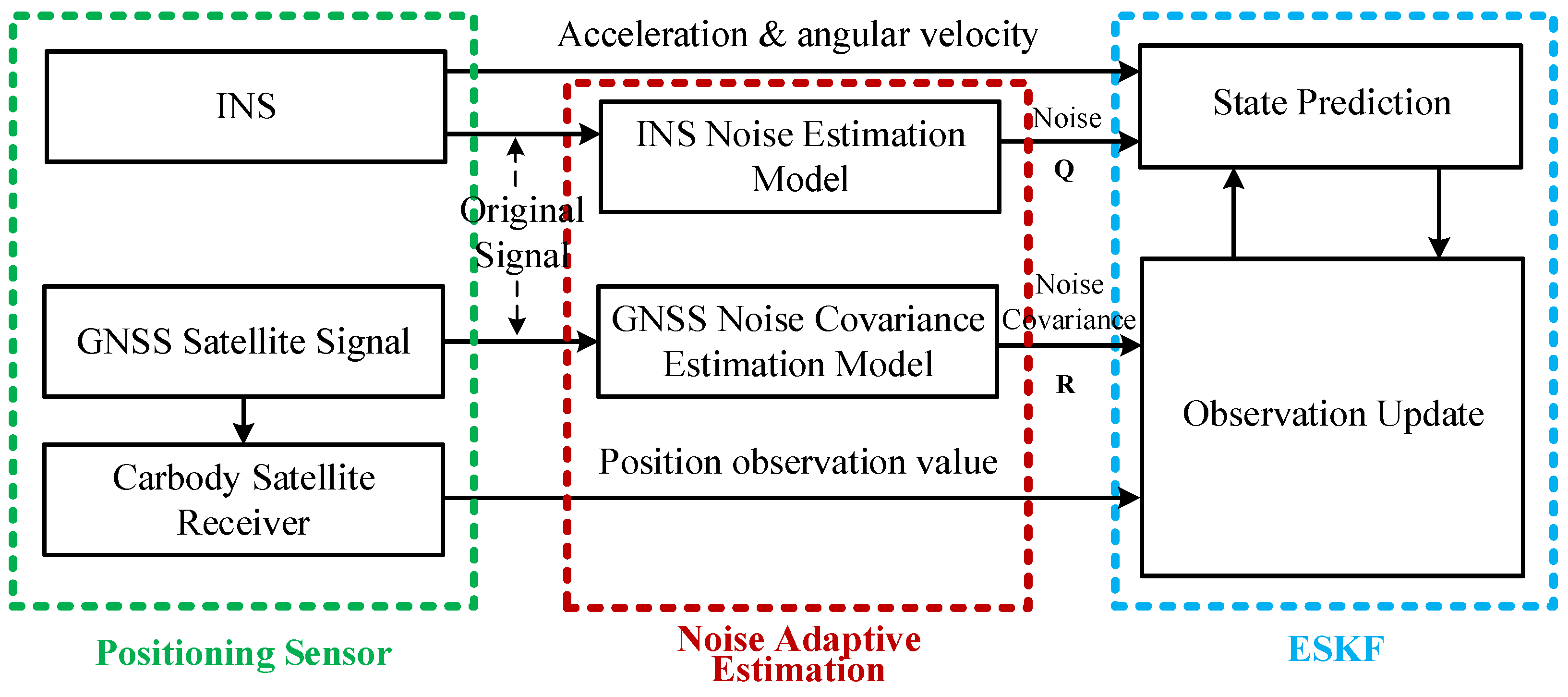
We integrate these adaptive noise estimates dynamically into an Error-State Kalman Filter. The estimated GNSS position uncertainty covariance matrix and INS process noise characteristics are used to update the observation noise covariance and process noise covariance matrices in real time, allowing the filter to autonomously balance sensor reliability under dynamic environmental conditions.

(3)

We conduct extensive field experiments demonstrating significant performance gains. The proposed GNSS noise model achieves 37.7% higher accuracy in quantifying positioning uncertainties compared to conventional elevation-based methods. Furthermore, the integrated GNSS/INS fusion positioning maintains an average absolute trajectory error of less than 0.6 m in challenging unstructured environments with intermittent GNSS outages, outperforming state-of-the-art fixed-weight fusion methods by 36.71% in positioning consistency. This framework effectively bridges the gap between theoretical sensor noise modeling and practical environmental adaptability for autonomous driving.

By bridging the gap between theoretical sensor fusion and practical environmental adaptability, this study advances the deployment of autonomous systems in real-world conditions where reliability cannot be compromised.

The remaining part of this paper is organized as follows. Section 2 reviews related work on multi-sensor fusion localization, adaptive noise estimation techniques, and robustness enhancement strategies. Section 3 details the proposed methodology. It elaborates on the noise covariance estimation model for satellite positioning (Section 3.1), the INS noise estimation model based on Allan variance analysis (Section 3.2), and the design of the noise-adaptive ESKF fusion algorithm (Section 3.3). Section 4 presents experimental verification and result analysis.

2. Related Research

Accurate localization in complex environments necessitates multi-sensor fusion. Recent research primarily focuses on three paradigms: filter-based fusion, factor graph optimization (FGO)-based fusion, and adaptive filtering techniques for dynamic noise handling. While the first two focus on the core fusion architecture, the third addresses the critical challenge of dynamically assessing sensor reliability within these architectures. This section systematically reviews key research in each category.

Filter-Based Fusion: These methods recursively estimate state (e.g., pose) using probabilistic models. Tan et al. [4] fused stereo vision and RTK-GPS using EKF. R-lins [5] employed an Iterated ESKF (IESKF) for lightweight LiDAR-inertial odometry. Xing et al. [6] proposed distributed weighted KF for unreliable networks; Jiang et al. [7] developed a fault-tolerant distributed framework; Gu et al. [8] used a federated KF for SINS/GNSS/odometry. Core Advantage: Computational efficiency for real-time applications. Key Limitation: Often assumes static noise characteristics, limiting adaptability.

FGO-Based Fusion: These methods represent states as nodes and sensor measurements/constraints as edges in a graph, optimized for global consistency. Lio-sam [9] tightly coupled LiDAR-inertial odometry with GPS and loop closures using FGO. LIO-mapping [10] used a sliding-window FGO for LiDAR-IMU fusion but faced real-time challenges. LVI-SAM [11] tightly coupled visual-inertial and LiDAR-inertial systems within a unified factor graph. Huang et al. [12] integrated dynamic covariance scaling (DCS) into FGO for robust AUV localization. Core Advantage: Effective incorporation of diverse constraints and potential for global consistency. Key Limitation: Higher computational cost, potentially impacting strict real-time performance.

Adaptive Filtering Techniques: These approaches dynamically estimate and adjust process noise and/or measurement noise covariances online to handle sensor degradation and changing environments. Methods include Variational/Innovation-based: Gao et al. [13] extended Variational Bayesian AKF (VB_AKF) to multi-sensor systems. Wang et al. [14] designed a Mahalanobis distance-based adaptive UKF. Measurement Difference/Residual-based: Duník et al. [15] introduced the Measurement Difference Autocovariance (MDAC) method. Random Weighting and Maximum Likelihood Estimators: Recent advances leverage random weighting theory and maximum likelihood principles to enhance noise estimation robustness. Gao et al. [16] proposed an adaptive random weighted H∞ estimator for system noise statistics, combining H∞ robustness with dynamic weight adjustment. Gao et al. [17] further developed a limited memory random-weighted Kalman filter (LM-RWKF) to suppress historical noise interference. Hu et al. [18] applied LM-RWKF to vehicle state estimation, demonstrating improved accuracy under dynamic conditions. For nonlinear systems, adaptive UKF variants integrating maximum posterior and random weighting [19] or windowing strategies [20] significantly improve estimation accuracy under uncertain noise. Moving Horizon and Covariance Estimation: Hu et al. [21] designed a UKF with process noise covariance estimation using maximum likelihood and moving horizon optimization for INS/GPS integration, effectively suppressing inertial drift. Similarly, Gao et al. [22] combined maximum likelihood with moving horizon estimation (MHE) to reduce computational load while maintaining noise adaptivity. Robust Variants: Duan et al. [23] proposed a robust adaptive EKF for tightly coupled INS/GPS. Yang et al. [24] introduced a chi-square test-based adaptive UKF (CAUKF) with adaptive thresholds for outlier detection in GNSS/INS fusion. Prior Noise Modeling (Allan Variance): Feng et al. [25] proposed Recursive Covariance Estimation (RCE). Narasimhappa et al. [26] improved Sage–Husa AKF (MSHARKF) with Allan variance modeling. Zhou et al. [27] developed an Allan variance-based adaptive algorithm for online measurement noise estimation. Hybrid/Weighting Methods: Shang et al. [28] optimized GNSS/INS fusion via hybrid a priori/posterior variance weighting. Ma et al. [29] investigated elevation-dependent noise in a multi-GNSS; Other Sensor Fusion: Martin et al. [30] fused CNN-derived pseudo-observations with IMU via EKF for dead reckoning.

As shown in

Table 1. Summary of key multi-sensor fusion localization methodologies.

Methodology	Core Mechanism	Representative Studies	Key Advantages	Main Limitations
Filter-Based	Recursive Bayesian estimation (e.g., KF, EKF, UKF, ESKF). Predict-Update cycle.	[4,5,6,7,8]	Computational efficiency, suitability for real-time applications, well-established theory.	Assumes fixed noise statistics, susceptible to error accumulation, sensitive to outliers/degradation (centralized).
FGO-Based	Formulate estimation as graph optimization. States as nodes, measurements as edges. Solve for optimal configuration.	[9,10,11,12]	Handles diverse constraints effectively, achieves global consistency, robust to local minima with loop closures.	Higher computational cost (especially for large graphs), potential challenges for strict real-time performance.
Adaptive Filtering	Dynamically estimate process (Q) and/or measurement (R) noise covariance online.	[13,14,15,16,17,18,19,20,21,22,23,24,25,26,27,28,29,30]	Enhances robustness to sensor degradation, environmental changes, and outliers. Improves accuracy under dynamic noise.	Estimation lag (especially posterior methods), sensitivity to initialization/tuning, potential complexity increase, may rely on specific noise models.

, while significant progress has been made in fusion architectures and adaptive noise estimation techniques, a gap remains in seamlessly integrating real-time, source-specific, and prior-informed noise modeling directly into the fusion filter to handle the dynamic error characteristics of heterogeneous sensors like GNSSs and INSs in complex, unstructured environments. Existing adaptive methods often exhibit hysteresis or lack direct physical modeling of dominant sensor error sources. Unlike data-driven approaches, our approach directly models the fundamental noise sources of GNSSs and INSs to construct a dual, real-time noise estimation framework. By leveraging these estimated prior noise characteristics to dynamically update both process and observation noise covariances within an ESKF, we specifically aim to overcome the hysteresis limitations of purely posterior error estimation methods, thereby enhancing the reliability and accuracy of GNSS/INS fusion under challenging conditions.

3. Proposed Approach

We propose a novel dual noise-adaptive framework for GNSS/INS fusion to achieve precise and reliable localization in complex, dynamic environments. The core innovation of this research lies in the development and integration of two real-time noise estimation models that dynamically calibrate sensor uncertainties: 1. GNSS uncertainty quantification: A hybrid model combining elevation-SNR joint prior weighting with Helmert variance component estimation for posterior residual compensation. This dual approach dynamically generates the observation noise covariance matrix, significantly improving uncertainty characterization over conventional single-source models. 2. INS noise estimation modeling: An Allan variance-based bias instability model within a sliding window, estimating time-dependent inertial sensor error growth to derive the process noise vector.

As illustrated in the system architecture (Figure 2), these adaptive noise models are tightly integrated into an Error-State Kalman Filter (ESKF): High-frequency INS measurements drive the prediction step, utilizing the dynamically estimated noise to update the process noise covariance Q. Upon receiving GNSS observations, the position measurement and its corresponding R matrix (derived from the hybrid noise model) are used for the observation update.

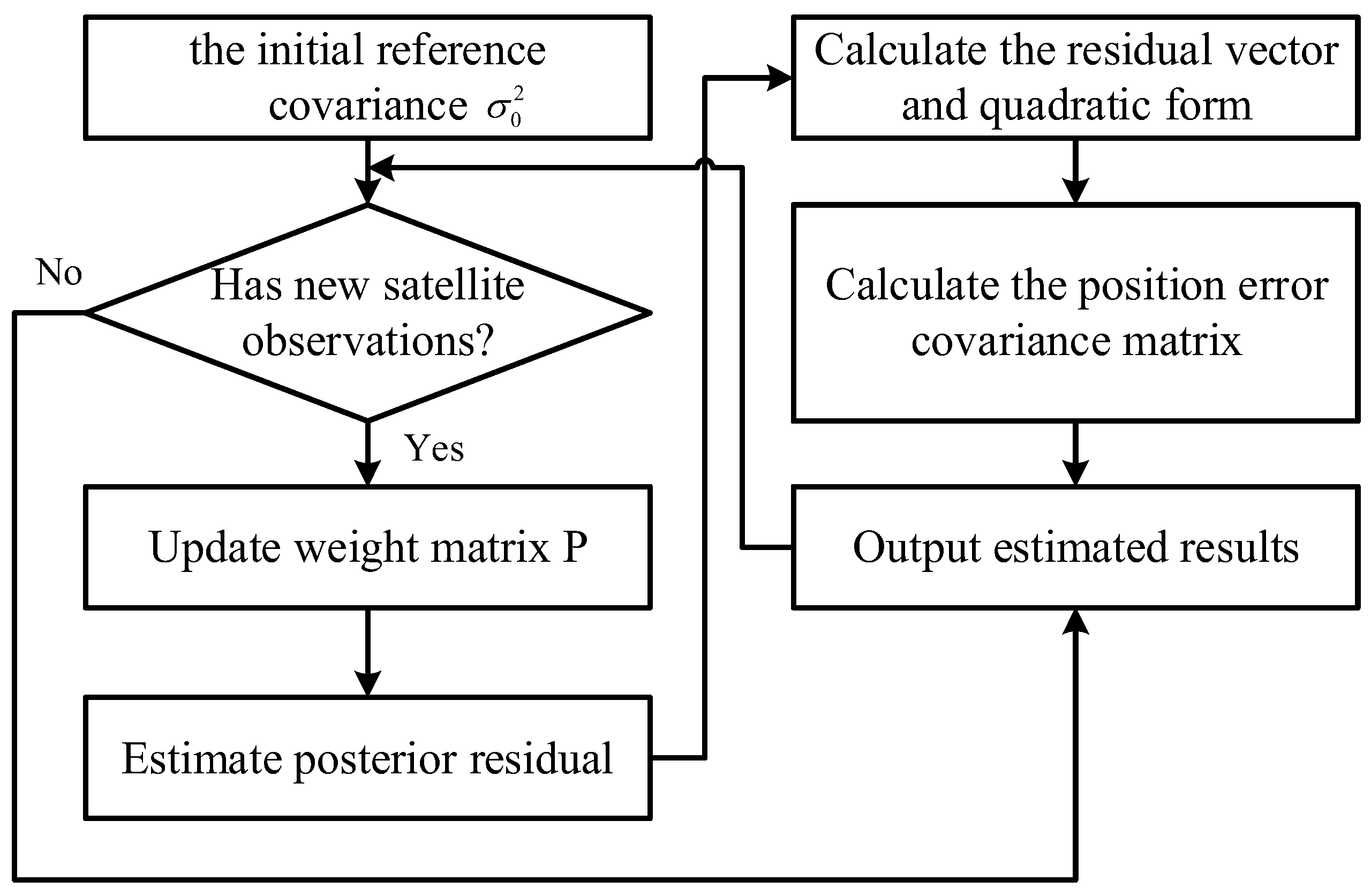
3.1. Noise Covariance Estimation Model for Satellite Positioning

The error sources in satellite navigation observations encompass satellite clock bias, ephemeris errors, relativistic effects, tropospheric delay, ionospheric delay, multipath effects, receiver clock bias, and other errors and noise. Accurately and comprehensively estimating noise from all sources in satellite positioning is exceedingly challenging. Starting from the mathematical formulation of pseudorange observation errors, an approximate expression for the error covariance matrix can be derived. This error covariance aligns in practical significance with the observation noise covariance, making the acquisition of this matrix the fundamental challenge in modeling.

As illustrated in Figure 3, satellite positioning resolves receiver coordinates through the spherical resection principle, using spatial distance spheres from multiple satellites. While the distance spheres of three satellites and the Earth’s surface theoretically intersect at a single point in space, time synchronization errors necessitate the observation of at least four satellites. A system of equations describing the geometric relationships between the receiver and multiple satellites is formulated to solve for pseudorange observations, where distinct numerical approaches to this overdetermined system yield varying positioning results. We employ the least squares method to compute single-point positioning solutions based on pseudorange measurements, optimizing parameter estimation through residual minimization.

Let the user’s true coordinates be $\left(x_u,y_u,z_u\right)$ and the coordinates of satellite $i$ be $\left(x_i,y_i,z_i\right)$. The pseudorange measured by receiver $r$ relative to satellite $i$ can be written as

$${\rho }_i^r=\sqrt{{\left(x_i-x_u\right)}^2+{\left(y_i-y_u\right)}^2+{\left(z_i-z_u\right)}^2}-cdT,$$

(1)

where ${\rho }_i^r$ represents the pseudorange measurement, $c$ is the speed of light, and $dT$ denotes the receiver clock error; this implies that as long as the positions of the receiver and satellite as well as the receiver’s clock error are known, the pseudorange measurement of a certain satellite can be obtained.

Since satellite positions can be provided by ephemeris, observations from at least four different satellites can estimate the user coordinates $\left(x_u,y_u,z_u\right)$ and receiver clock bias $dT$. Using these estimates, the estimated value of pseudorange ${\widehat{\rho }}_i$ can be obtained as

$${\widehat{\rho }}_i=\sqrt{{\left(x_i-{\widehat{x}}_u\right)}^2+{\left(y_i-{\widehat{y}}_u\right)}^2+{\left(z_i-{\widehat{z}}_u\right)}^2}-cd\widehat{T},$$

(2)

where $x_u={\widehat{x}}_u+\mathsf{\Delta }{x}_u,y_u={\widehat{y}}_u+\mathsf{\Delta }{y}_u, z_u={\widehat{z}}_u+\mathsf{\Delta }{z}_u,dT=d\widehat{T}+\mathsf{\Delta }{t}_u,{\widehat{\mathrm{x}}}_{\mathrm{u}},{\widehat{\mathrm{y}}}_{\mathrm{u}},{\widehat{\mathrm{z}}}_{\mathrm{u}}, \mathrm{and} d\widehat{T}$ are all estimated values, and $\mathsf{\Delta }{x}_u, \mathsf{\Delta }{y}_u, \mathsf{\Delta }{z}_u, \mathrm{and} \mathsf{\Delta }{t}_u$ are corresponding estimated errors. This implies that the satellite estimation error is only related to the estimated values of each variable and the satellite position. Expanding the new pseudorange measurement equation using a first-order Taylor series yields

$${\rho }_i={\widehat{\rho }}_i+{\displaystyle \frac{\partial {\widehat{\rho }}_i}{\partial {\widehat{x}}_u}}\mathsf{\Delta }{x}_u+{\displaystyle \frac{\partial {\widehat{\rho }}_i}{\partial {\widehat{y}}_u}}\mathsf{\Delta }{y}_u+{\displaystyle \frac{\partial {\widehat{\rho }}_i}{\partial {\widehat{z}}_u}}\mathsf{\Delta }{z}_u+{\displaystyle \frac{\partial {\widehat{\rho }}_i}{\partial \left(d\widehat{T}\right)}}\mathsf{\Delta }{t}_u+\dots ,$$

(3)

where

$$\begin{gathered} {\displaystyle \frac{\partial {\widehat{\rho }}_i}{\partial {\widehat{x}}_u}}=-{\displaystyle \frac{x_i-{\widehat{x}}_u}{\sqrt{{\left(x_i-{\widehat{x}}_u\right)}^2+{\left(y_i-{\widehat{y}}_u\right)}^2+{\left(z_i-{\widehat{z}}_u\right)}^2}}} \\ {\displaystyle \frac{\partial {\widehat{\rho }}_i}{\partial {\widehat{y}}_u}}=-{\displaystyle \frac{y_i-{\widehat{y}}_u}{\sqrt{{\left(x_i-{\widehat{x}}_u\right)}^2+{\left(y_i-{\widehat{y}}_u\right)}^2+{\left(z_i-{\widehat{z}}_u\right)}^2}}} \\ {\displaystyle \frac{\partial {\widehat{\rho }}_i}{\partial {\widehat{z}}_u}}=-{\displaystyle \frac{z_i-{\widehat{z}}_u}{\sqrt{{\left(x_i-{\widehat{x}}_u\right)}^2+{\left(y_i-{\widehat{y}}_u\right)}^2+{\left(z_i-{\widehat{z}}_u\right)}^2}}} \\ {\displaystyle \frac{\partial {\widehat{\rho }}_i}{\partial \left(d\widehat{T}\right)}}=-c \end{gathered}$$

(4)

When the number of satellites exceeds three, according to Equation (3), the matrix form of the simultaneous observation equations can be written as

$$\mathsf{\Delta }\rho =H\mathsf{\Delta }x,$$

(5)

where

$$\mathsf{\Delta }p=\left[\begin{array}{c}{\rho }_1-{\widehat{\rho }}_1\\ {\rho }_2-{\widehat{\rho }}_2\\ ⋮\\ {\rho }_n-{\widehat{\rho }}_n\end{array}\right],H=\left[\begin{array}{cccc}{\displaystyle \frac{\partial {\widehat{\rho }}_1}{\partial {\widehat{x}}_u}}& {\displaystyle \frac{\partial {\widehat{\rho }}_1}{\partial {\widehat{y}}_u}}& {\displaystyle \frac{\partial {\widehat{\rho }}_1}{\partial {\widehat{z}}_u}}& -1\\ {\displaystyle \frac{\partial {\widehat{\rho }}_2}{\partial {\widehat{x}}_u}}& {\displaystyle \frac{\partial {\widehat{\rho }}_2}{\partial {\widehat{y}}_u}}& {\displaystyle \frac{\partial {\widehat{\rho }}_2}{\partial {\widehat{z}}_u}}& -1\\ ⋮& ⋮& ⋮& ⋮\\ {\displaystyle \frac{\partial {\widehat{\rho }}_n}{\partial {\widehat{x}}_u}}& {\displaystyle \frac{\partial {\widehat{\rho }}_n}{\partial {\widehat{y}}_u}}& {\displaystyle \frac{\partial {\widehat{\rho }}_n}{\partial {\widehat{z}}_u}}& -1\end{array}\right],\mathsf{\Delta }x=\left[\begin{array}{c}\mathsf{\Delta }{x}_u\\ \mathsf{\Delta }{y}_u\\ \mathsf{\Delta }{z}_u\\ c\mathsf{\Delta }{t}_u\end{array}\right]$$

(6)

The least squares solution is

$$\mathsf{\Delta }x={\left(H^{T}H\right)}^{-1}{H}^T\mathsf{\Delta }\rho$$

(7)

This implies that the solution of satellite estimation error requires pseudorange observations from at least four satellites, and the determination of satellite estimation error lays the foundation for us to derive the covariance matrix of satellite observations in the following text.

After considering the measurement errors of each satellite, since these errors vary across satellites and assuming they are mutually independent, the weight matrix $P$ is introduced. After introducing matrix $P$, Equation (7) becomes

$$\mathsf{\Delta }x={\left(H^{T}PH\right)}^{-1}{H}^{T}P\mathsf{\Delta }\rho ,$$

(8)

where $P=\mathrm{diag}\left(1/{\sigma }_1^2, 1/{\sigma }_2^2,\dots ,1/{\sigma }_i^2,\dots ,1/{\sigma }_n^2\right)$, and ${\sigma }_i^2$ represents the variance of the measurement error for satellite $i$. This implies that the solution of satellite estimation error is associated with the observation error of each satellite.

Therefore, the covariance matrix of the error quantity $\mathsf{\Delta }\mathrm{x}$ is obtained as

$$\mathrm{cov}\left(\mathsf{\Delta }x\right)=E\left\{\mathsf{\Delta }x\mathsf{\Delta }{x}^T\right\}={\left(H^{T}PH\right)}^{-1}{H}^{T}PE\left\{\mathsf{\Delta }\rho \left(\mathsf{\Delta }{\rho }^T\right)\right\}{P}^{T}H{\left(H^T{P}^{T}H\right)}^{-1}$$

(9)

If the position of satellite $i$ relative to the user is represented by the azimuth angle ($A{z}_i$, measured clockwise from true north) and the elevation angle ($E{l}_i$, relative to the horizontal plane,$0^{\circ }<El<{90}^{\circ }$), then the matrix $H$ can be rewritten as [31]

$$\mathrm{H}=\left[\begin{array}{cccc}\cos \left(E{l}_1\right)\sin \left(A{z}_1\right)& \cos \left(E{l}_1\right)\cos \left(A{z}_1\right)& \sin \left(E{l}_1\right)& 1\\ \cos \left(E{l}_2\right)\sin \left(A{z}_2\right)& \cos \left(E{l}_2\right)\cos \left(A{z}_2\right)& \sin \left(E{l}_2\right)& 1\\ ⋮& ⋮& ⋮& ⋮\\ \cos \left(E{l}_n\right)\sin \left(A{z}_n\right)& \cos \left(E{l}_n\right)\cos \left(A{z}_n\right)& \sin \left(E{l}_n\right)& 1\end{array}\right]$$

(10)

This implies that in a real satellite positioning environment, the matrix H can be obtained by measuring the azimuth and elevation angles of each satellite without the need to calculate complex partial derivatives.

As satellite signals are subject to complex influences such as the ionosphere, troposphere, and multipath effects during propagation, the covariance levels of observations for each satellite inevitably differ, and these differences vary over time. The weight matrix $P$ measures the observation quality of each satellite and must, therefore, be updated each time new observations are obtained.

We evaluate the observation accuracy and quality of each satellite from two perspectives.

First, the elevation angle of the observed satellite. Satellites at different elevation angles are affected differently by the ionosphere, troposphere, and multipath effects. Low-elevation satellites, which must pass through thicker atmospheric layers, experience significantly greater atmospheric refraction effects than high-elevation satellites, resulting in larger observation noise. Li proposed a stochastic model based on the sine function of the satellite elevation angle [32]:

$${\sigma }_i={\displaystyle \frac{1}{\sin a_i}},$$

(11)

where $\sigma$ and $a$ represent the error in the original observation of satellite $\mathrm{i}$ and its elevation angle, respectively.

Based on extensive statistical observation data, we propose an improved model based on the satellite elevation angle:

$${\sigma }_i^2={\sigma }_0^2{\displaystyle \frac{1.1}{\sin \left(E{l}_i\right)+0.1}},$$

(12)

where ${\sigma }_0^2$ is the initial reference covariance of satellite $\mathrm{i}$, and $E{l}_i$ denotes its elevation angle.

The second aspect is the signal-to-noise ratio (SNR) of observation satellites. SNR refers to the ratio of the received carrier signal strength to the noise strength, typically expressed as the carrier-to-noise density power ratio $\left(\mathrm{C}/{\mathrm{N}}_0\right)$. When multipath or obstruction occurs, the SNR value changes accordingly, reflecting the accuracy level of observations more effectively than the satellite elevation angle model. However, not all receivers can output standard SNR. Official data format documents often use signal strength as a substitute for SNR. Signal strength is essentially the projection of SNR observations onto the interval $\left[1,9\right]$. A higher value indicates better observation quality, with 5 being the critical threshold. A signal strength greater than 5 signifies lower observation noise, while a value below 5 indicates higher observation noise. This model is represented using a piecewise function [33]:

$${\sigma }_i^2=\left\{\begin{array}{l}{\sigma }_0^2{\left({\displaystyle \frac{sg/str}{9}}\right)}^3,1\le sg/str\le 4\hfill \\ {\sigma }_0^2{\left({\displaystyle \frac{sg/str}{9}}\right)}^2,5\le sg/str\le 7\hfill \\ {\sigma }_0^2\left({\displaystyle \frac{sg/str}{9}}\right),8\le sg/str\le 9\hfill \end{array}\right.,$$

(13)

where ${\sigma }_0^2$ is the initial reference covariance of satellite $\mathrm{i}$, and $\mathrm{sg}/\mathrm{str}$ represents the signal strength.

Generally, the satellite SNR value decreases steadily as the elevation angle decreases. However, in real-world complex positioning scenarios, the two aforementioned aspects may fail independently. For example, a high SNR may occur at low satellite elevation angles, and satellites directly overhead may still be affected by multipath effects. Using a single stochastic model may not accurately assess the observation quality of satellites. Therefore, we propose and establish a joint stochastic model combining satellite elevation angles and SNR:

$${\sigma }_i^2=\left\{\begin{array}{l}{\sigma }_0^2{\left({\displaystyle \frac{sg/str}{9}}\right)}^3{\displaystyle \frac{1.1}{\sin \left(E{l}_i\right)+0.1}},1\le sg/str\le 4\hfill \\ {\sigma }_0^2{\left({\displaystyle \frac{sg/str}{9}}\right)}^2{\displaystyle \frac{1.1}{\sin \left(E{l}_i\right)+0.1}},5\le sg/\mathrm{str}\le 7\hfill \\ {\sigma }_0^2\left({\displaystyle \frac{sg/str}{9}}\right){\displaystyle \frac{1.1}{\sin \left(E{l}_i\right)+0.1}},8\le sg/\mathrm{str}\le 9\hfill \end{array}\right.$$

(14)

This implies that this model accounts for the combined influence of satellite elevation angles and SNR, mitigating the impact of signal diffraction and non-ideal stochastic characteristics on observation quality estimation. The weight matrix $P$ is updated based on the joint stochastic model.

For $E\left\{\mathsf{\Delta }p\left(\mathsf{\Delta }{p}^T\right)\right\}$ in Equation (9), it actually represents the covariance of pseudorange residuals. This paper employs a posterior variance estimation method to calculate it. Based on the principle of least squares, an error equation is introduced:

$$V=H\mathsf{\Delta }\widehat{x}-\mathsf{\Delta }\rho$$

(15)

The calculation of matrix $V$ can be obtained through posterior estimation of $\mathsf{\Delta }x$. After incorporating the weight matrix, the quadratic form $V^{T}PV$ of the residual vector $V$ is used to estimate the covariance of pseudorange residuals. The quadratic form $V^{T}PV$ describes the deviation between posterior estimates and prior observations. According to Helmert’s variance estimation method,

$$E\left\{\mathsf{\Delta }\rho \left(\mathsf{\Delta }{\rho }^T\right)\right\}={\displaystyle \frac{V^{T}PV}{n-\mathrm{tr}\left(H^{T}PH\right)}},$$

(16)

where $n$ represents the total number of satellites observed by the GPS, GLONASS, and BDS systems (we adopted the single difference method), and $\mathrm{tr}$ represents the trace of the matrix.

Combining and simplifying Equation (9) yields

$$\mathrm{cov}\left(\mathsf{\Delta }x\right)={\left(H^{T}PH\right)}^{-1}{\displaystyle \frac{V^{T}PV}{n-\mathrm{tr}\left(H^{T}PH\right)}}$$

(17)

This implies that based on our previous calculation methods for matrices $\mathrm{H}$ and $\mathrm{P}$ and residual vector $\mathrm{V}$, the covariance matrix of the position error can be easily calculated. The covariance matrix $\mathrm{cov}\left(\mathsf{\Delta }x\right)$ describes the accuracy of GNSS single-point positioning, which can be used as an indicator to evaluate satellite positioning errors or as a covariance parameter to directly participate in real-time noise estimation in integrated navigation.

As illustrated in Figure 4, the satellite positioning noise estimation algorithm operates as follows. The process begins by determining the initial reference covariance ${\sigma }_0^2$ for each satellite, leveraging pseudorange accuracy metrics and empirical data. Concurrently, the covariance value ${\sigma }_0^2$ quantifying the observation quality of satellite i is computed using the joint stochastic model (Equation (14)), which dynamically integrates the current elevation angle $\left(E{l}_i\right)$ and SNR of all observed satellites. This covariance value updates the weight matrix $P$ to reflect real-time observation uncertainties. Subsequently, a weighted least squares estimation is performed according to Equation (8), yielding the posterior residual $\mathsf{\Delta }x$. The residual vector $V$ is then derived from the error equation (Equation (15)), enabling the computation of the quadratic form $V$ to quantify deviations between posterior estimates and prior observations. Finally, the Helmert variance component estimation method (Equation (16)) is applied to calculate the covariance of pseudorange residuals, $E\left\{\mathsf{\Delta }\rho \left(\mathsf{\Delta }{\rho }^T\right)\right\}$. This posterior refinement, combined with the updated weight matrix $P$ and geometry matrix $H$, directly yields the position error covariance matrix $\mathrm{cov}\left(\mathsf{\Delta }x\right)$ for GNSS single-point positioning through Equation (17). This covariance matrix characterizes the spatial uncertainty of the GNSS solution and serves as a critical input for adaptive fusion.

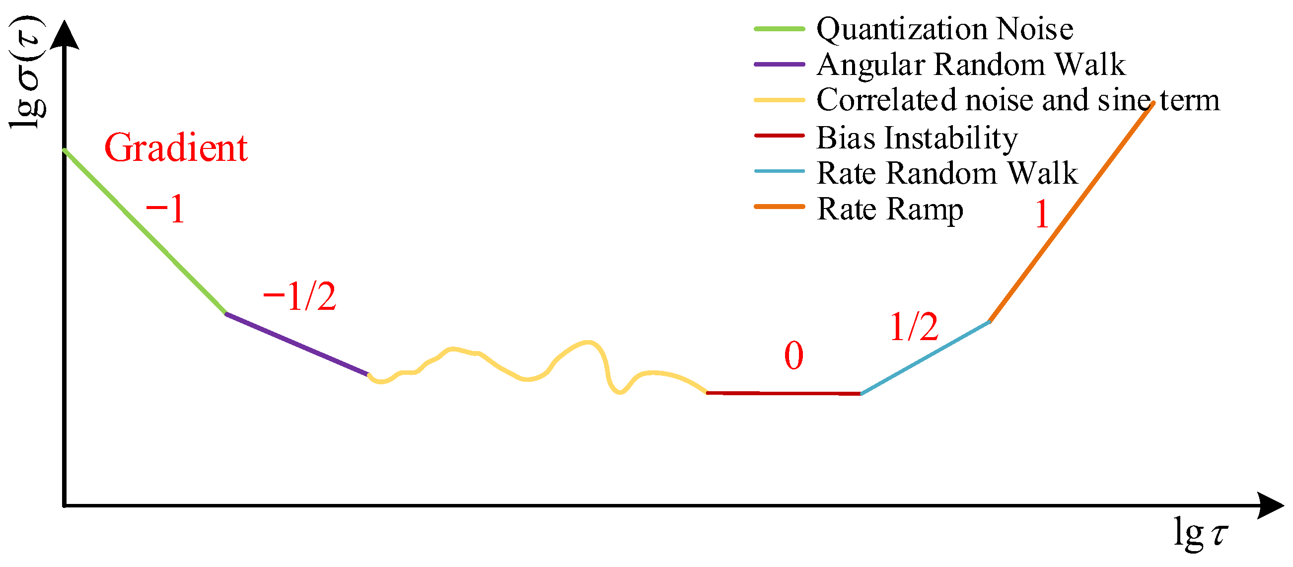
3.2. INS Noise Estimation Model Based on Allan Variance Analysis

When the INS continuously updates system state variables at high frequencies, the resulting errors and noise require accurate estimation and timely compensation. We utilize Allan variance analysis for the identification and estimation of INS noise.

As a time-domain analysis technique, the Allan variance method can thoroughly characterize and identify the statistical properties of various error sources. Assuming $t_0$ gyroscope data points are collected within the sampling period, these $N$ data points are evenly divided into $K$ groups, with each group containing $n$ sampling points (typically $\left.n=2^i,i=0,1,2\dots \right)$. The group average is ${\stackrel{-}{\omega }}_k\left(n\right)={\displaystyle \frac{1}{n}}{\displaystyle \sum }_1^n{\omega }_{\left(k-1\right)n+1},k=1,2,\dots ,K$. The definition of Allan variance can then be written as [34]

$${\sigma }_A^2\left(T\right)={\displaystyle \frac{1}{2}}〈{\left[{\stackrel{-}{\omega }}_{k+1}\left(n\right)-{\stackrel{-}{\omega }}_k\left(n\right)\right]}^2〉\cong {\displaystyle \frac{1}{2\left(K-1\right)}}{{\displaystyle \sum }}_{k=1}^{K-1}{\left[{\stackrel{-}{\omega }}_{k+1}\left(n\right)-{\stackrel{-}{\omega }}_k\left(n\right)\right]}^2,$$

(18)

where $\mathrm{T}={\mathrm{nt}}_0$, and the symbol $〈•〉$ represents the overall average. This implies that the Allan variance can be estimated by accumulating data variations over a period (specifically, the overall average of adjacent data segments), thereby distinguishing and separating noise within the sequence. It essentially leverages the statistical properties of noise over a long period.

The physical meaning and application of Allan variance for random signals fundamentally stem from its relationship with the power spectral density (PSD, signal power per unit frequency band, which describes how signal power varies with frequency, i.e., the distribution of signal power in the frequency domain). If multiple random processes are independent, their power spectra satisfy the property of linear additivity. Therefore, when plotting the “time interval–variance double logarithmic curve” (where time interval is the reciprocal of frequency, and variance is the integral of the power spectrum), the resulting curve slopes will necessarily differ. The INS consists of gyroscopes and accelerometers, and its potential noise sources during operation mainly include quantization noise, angle random walk, angular rate random walk, bias instability, and rate ramp, all of which are mutually independent. Thus, Allan variance analysis can be employed for noise identification and estimation.

For quantization noise $Q$, its angular rate quantization noise power spectrum is $S_{QN}\left(f\right)={\tau }_0{Q}^2{\left(2\pi f\right)}^2$. Combining the continuous form of Equation (18) and setting the time interval as $\tau$, its double logarithmic expression is

$$lo{g}_{10}{\sigma }_{QN}\left(\tau \right)=lo{g}_{10}\sqrt{3}Q-lo{g}_{10}\tau$$

(19)

For angular random walk $N$, its angular rate power spectrum is a constant, i.e., $S_{ARW}\left(f\right)=N^2$. Thus, its double logarithmic expression is

$$lo{g}_{10}{\sigma }_{ARW}\left(\tau \right)=lo{g}_{10}N-{\displaystyle \frac{1}{2}}lo{g}_{10}\tau$$

(20)

For rate random walk $K$, its acceleration power spectrum is also a constant, so its double logarithmic expression is

$$lo{g}_{10}{\sigma }_{RRW}\left(\tau \right)=lo{g}_{10}\left(K/\sqrt{3}\right)+{\displaystyle \frac{1}{2}}lo{g}_{10}\tau$$

(21)

For bias instability $B$, the angular rate power spectrum of bias instability noise is $S_{\mathsf{\Omega }}\left(f\right)=B^2/\left(2\pi f\right)$. Therefore, its double logarithmic expression is

$$lo{g}_{10}{\sigma }_{BI}\left(\tau \right)=lo{g}_{10}\left(2B/3\right)$$

(22)

For rate ramp $R$, the angular rate $\mathsf{\Omega }$ exhibits a linear relationship with the test time $t$, i.e., $\mathsf{\Omega }\left(t\right)=\mathsf{\Omega }\left(0\right)+Rt$. Hence,

$$lo{g}_{10}{\sigma }_{RR}\left(\tau \right)=lo{g}_{10}\left(R/\sqrt{2}\right)+lo{g}_{10}\tau$$

(23)

Analysis based on Formulas (19)–(23) reveals that the corresponding slopes of each random noise in the “variance versus time interval log–log curve” are sequentially $-1, -1/2, 0, 1/2, 1$, with the general shape of the curve shown in Figure 5. Effective identification of various noise types can be achieved through these slopes.

Let $\tau =1$, i.e., find the intersection of the log–log curve with the line $\tau =1$, yielding

$$\begin{gathered} Q=\sqrt{3}\sigma \left(1\right)/3 \\ N=\sigma \left(1\right) \\ K=\sqrt{3}\sigma \left(1\right) \\ B=3\sigma \left(1\right)/2 \\ R=\sqrt{2}\sigma \left(1\right) \end{gathered}$$

(24)

We establish a sliding window to estimate the noise of the gyroscope and accelerometer in real time. Specifically, by selecting the raw outputs of the gyroscope and accelerometer from the past $\mathsf{\Delta }T$ time and using the discrete form of Equation (18), we obtain the Allan variance curve ${\sigma }^2\left(T\right)$. Calculating $\sigma \left(1\right)$ allows rapid estimation of various noise types over the $\mathsf{\Delta }T$ time period.

While Allan variance analysis traditionally requires static data, our sliding-window approach targets slow-varying noise components (e.g., bias instability) whose timescales exceed typical vehicle dynamics. The following are used to mitigate motion artifacts:

(a)

Raw IMU data are pre-filtered with a 20 Hz high-pass filter to remove suspension-induced vibrations [19];

(b)

Noise estimation is suspended during aggressive maneuvers (lateral acceleration >2 m/s² or angular rate > 10°/s).

This ensures dynamics-induced signals do not dominate the Allan variance profile.

3.3. ESDF-Based State Estimation Using Noise Model

The primary task of fusion positioning is to combine information from multiple sensors in space or time according to certain criteria, thereby obtaining a consistent description of the target state. We employ an error-state Kalman filter (ESKF) algorithm to integrate data from different sources for vehicle state estimation. The ESKF uses the accumulated error increments of the nominal state as the system state variables, employing local linearization to estimate the error state and correct the nominal state. Compared to a standard Kalman filter, the error-state parameters are minimized (the number of parameters equals the degrees of freedom), effectively avoiding risks such as over-parameterization and singularity in the covariance matrix. We continuously predict and update the system state using high-frequency angular velocity and acceleration data from the INS, while observation corrections are performed using satellite positioning information from the GNSS, achieving efficient and orderly fusion of redundant information.

As shown in Figure 6, we couple the previously constructed GNSS and INS noise estimation models with the filtering algorithm, designing the model outputs as the process noise and observation noise of the filter, which are updated alongside the prediction and observation processes. This enables dynamic adaptive adjustment of the “weights” of each module involved in the fusion, reducing the impact of unreliable observations. In the figure, because the estimation error of GNSS positioning for elevation is significantly larger than that for horizontal positioning, the GNSS error ellipse (red ellipse) appears vertically elongated. The cumulative error of INS positioning is generally only related to time, so its error increases as the vehicle moves. The gray ellipse actually represents the state error covariance matrix of the Kalman filter, reflecting the filter’s uncertainty in estimating the system state. When the noise characteristics of both the GNSS and INS are accurately estimated, the system state error covariance actually decreases. This demonstrates the characteristic of the Kalman filter providing optimal state estimation. That is, even if the INS or GNSS data become unreliable, the estimation remains robust, and the uncertainty in the vehicle’s own position reduces.

3.3.1. State Equation Construction

The state prediction and update process relies on real-time measurements of angular velocity and acceleration from the INS. We select error increments for position, velocity, attitude, acceleration bias, and angular velocity bias $\delta P$, $\delta V$, $\delta \theta$, $\delta b_a$, and $\delta b_{\omega }$, respectively, as the system state variables $\delta x$, i.e.,

$$\delta x={\left[\begin{array}{lllll}\delta P\hfill & \delta V\hfill & \delta \theta \hfill & \delta b_a\hfill & \delta b_{\omega }\hfill \end{array}\right]}^T$$

(25)

Unlike the standard Kalman filter, which directly uses the nominal state as the system state, the ESKF employs the error increment accumulated by the nominal state as the system state—that is, the bias between the true value and the estimated value—and utilizes local linearization to estimate the error state and correct the nominal state. Considering the singularity that may occur when using Euler angles to represent attitude, we actually use the rotation matrix to represent attitude $\theta$ uniformly.

Under the assumption of linear Gaussianity, the error equation can be written in the general form of the state equation:

$$\delta \dot{x}=F_t\delta x+B_{t}w,$$

(26)

where $w={\left[\begin{array}{llll}{n}_a\hfill & n_{\omega }\hfill & n_{b_a}\hfill & n_{b_{\omega }}\hfill \end{array}\right]}^{\mathrm{T}}$ represents the device noise of the accelerometer and gyroscope, also known as process noise, including the output noise and bias noise of the INS. We update it using the INS noise estimation model from Section 3.2:

$$\begin{gathered} w={\left[\begin{array}{llll}{n}_a\hfill & n_{\omega }\hfill & n_{b_a}\hfill & n_{b_{\omega }}\hfill \end{array}\right]}^T \\ ={\left[\begin{array}{llll}{Q}_a+N_a+R_a\hfill & Q_{\omega }+N_{\omega }+K_{\omega }+R_{\omega }\hfill & B_a\hfill & B_{\omega }\hfill \end{array}\right]}^T, \end{gathered}$$

(27)

where $Q_a={\left[{\mathrm{Q}}_{\mathrm{a}}^{\mathrm{x}},{\mathrm{Q}}_{\mathrm{a}}^{\mathrm{y}},{\mathrm{Q}}_{\mathrm{a}}^{\mathrm{z}}\right]}^{\mathrm{T}}$ denotes the values of quantization noise on the three axes of the accelerometer $\mathrm{xyz}$, while expressions for other noise components on the three axes $\mathrm{xyz}$ are similar to $Q_a$. This allows us to compute $\mathrm{w}$ in real time using the Allan variance curves for each axis and Equation (24).

The state transition matrix $F_t$ and the process noise coefficient matrix $B_t$ are, respectively,

$$\begin{gathered} F_t=\left[\begin{array}{ccccc}\mathbf{0}& I_3& \mathbf{0}& \mathbf{0}& \mathbf{0}\\ \mathbf{0}& \mathbf{0}& -R_t{\left[{\overline{a}}_t\right]}_{\times }& -R_t& \mathbf{0}\\ \mathbf{0}& \mathbf{0}& -{\left[{\overline{\omega }}_t\right]}_{\times }& \mathbf{0}& -I_3\\ \mathbf{0}& \mathbf{0}& \mathbf{0}& \mathbf{0}& \mathbf{0}\\ \mathbf{0}& \mathbf{0}& \mathbf{0}& \mathbf{0}& \mathbf{0}\end{array}\right] \\ {B}_t=\left[\begin{array}{cccc}\mathbf{0}& \mathbf{0}& \mathbf{0}& \mathbf{0}\\ R_t& \mathbf{0}& \mathbf{0}& \mathbf{0}\\ \mathbf{0}& I_3& \mathbf{0}& \mathbf{0}\\ \mathbf{0}& \mathbf{0}& I_3& \mathbf{0}\\ \mathbf{0}& \mathbf{0}& \mathbf{0}& I_3\end{array}\right], \end{gathered}$$

(28)

where ${\overline{a}}_t={\overline{\mathrm{a}}}_{\mathrm{t}}=a_t-b_{a_t},{\overline{\omega }}_t={\omega }_{\mathrm{t}}-b_{{\omega }_t}.$ $R_t$ represents the carrier rotation matrix at time $\mathrm{t}$, ${\left[{\overline{\omega }}_t\right]}_{\times }$ denotes the skew-symmetric matrix corresponding to the carrier angular velocity vector ${\overline{\omega }}_t$ at time $\mathrm{t}$, i.e., ${\left[{\overline{\omega }}_t\right]}_{\times }=\left[\begin{array}{ccc}0& -{\mathsf{\omega }}_3& {\mathsf{\omega }}_2\\ {\mathsf{\omega }}_2& 0& -{\mathsf{\omega }}_1\\ -{\mathsf{\omega }}_2& {\mathsf{\omega }}_1& 0\end{array}\right],$ ${\overline{a}}_t$ represents the carrier acceleration vector at time $\mathrm{t}$, and $I_3$ indicates the third-order identity matrix.

When the INS outputs the carrier’s angular velocity and acceleration information, the inertial solution completes the prediction update of the filter through the error state equation, while the updated accelerometer bias and gyroscope bias compensate for the acceleration and angular velocity in the next iteration. The corrected nominal state quantity $x_{k+1}$ in the carrier frame at time $k+1$ is

$$x_{k+1}=x_k\oplus \delta \widehat{x}=\left[\begin{array}{c}{P}_k+\delta {\widehat{p}}_k\\ V_k+\delta {\widehat{v}}_k\\ {\theta }_k·\exp \left(\delta {\widehat{\theta }}_k\right)\\ b_k+\delta {\widehat{b}}_a\\ b_a+\delta {\widehat{b}}_a\end{array}\right],$$

(29)

where the symbol $\oplus$ denotes the superposition of state quantities, and $\delta \widehat{x}$, $\delta {\widehat{p}}_k$, $\delta {\widehat{v}}_k$, $\delta {\widehat{\theta }}_k$, $\delta {\widehat{b}}_a$, and $\delta {\widehat{b}}_a$ represent the estimated values of the filter for each system state variable at the time $k$, and $x_k$, $P_k$, $V_k$, ${\theta }_k$, $b_k$ and $b_a$ respectively represent the corresponding nominal state quantities.

3.3.2. Observation Equation Construction

The observation equation is generally written as

$$y=G_t\delta x+C_{t}n,$$

(30)

We use the position observation from GNSS measurements, i.e., $y=\delta \overline{p}$. Thus, the observation matrix $G_t$ and the observation noise coefficient matrix $C_t$ are

$$\begin{gathered} G_t=\left[\begin{array}{lllll}{I}_3\hfill & \mathbf{0}\hfill & \mathbf{0}\hfill & \mathbf{0}\hfill & \mathbf{0}\hfill \end{array}\right] \\ {C}_t=I_3, \end{gathered}$$

(31)

At this point, the observation noise is $n\in R^N\sim \mathcal{N}\left(0,R_{GNSS}\right)$, and $n={\left[\begin{array}{lll}{n}_{\delta {\stackrel{-}{p}}_x}\hfill & n_{\delta {\stackrel{-}{p}}_y}\hfill & n_{\delta {\stackrel{-}{p}}_z}\hfill \end{array}\right]}^T$. The noise covariance matrix $R_{GNSS}$ also measures the uncertainty of the GNSS position observation. We dynamically update the matrix $R_{GNSS}$ using the noise covariance estimation model from Section 3.1:

$$R_{GNSS}\propto \mathrm{cov}\left(\mathsf{\Delta }x\right)\Rightarrow R_{GNSS}=\lambda \mathrm{cov}\left(\mathsf{\Delta }x\right),$$

(32)

where $\lambda$ is the scaling factor. The scaling factor $\mathsf{\lambda }$ is mainly used to unify the magnitude of GNSS noise estimation and INS noise estimation output results, ensuring the correct weighting of filters. We utilize the initial static phase of the system to determine $\mathsf{\lambda }$ (the first 200 s after INS startup when the vehicle is stationary). During this phase, we firstly compute the average trace ${\mathrm{tr}}_{\mathrm{gnss}}$ of the GNSS position error covariance matrix $\mathrm{cov}\left(\mathsf{\Delta }\mathrm{x}\right)$ under open-sky conditions. Then, we compute the average trace ${\mathrm{tr}}_{\mathrm{ins}}$ of the angular velocity random walk matrix ${\mathrm{K}}_{\mathsf{\omega }}$ and bias instability matrix ${\mathrm{B}}_{\mathsf{\omega }}$ (dominant error in static mode). Thus, we obtain the scaling factor $\mathsf{\lambda }={\mathrm{tr}}_{\mathrm{ins}}/{\mathrm{tr}}_{\mathrm{gnss}}$.

With the state equation and observation equation in place, we follow the general ESKF process to update the vehicle’s state, while the noise estimation model simultaneously outputs the estimated noise results of each sensor to the filter. The workflow of the GNSS/INS fusion positioning algorithm based on ESKF is illustrated in Figure 7.

4. Experimental Verification and Result Analysis

4.1. Experimental Platform and Methods

As shown in Figure 8, our experimental validation hardware platform is equipped with a Hesai-64 3D LiDAR (Made by Hesai Technology in Shanghai, China) sensor installed on the vehicle’s roof, which provides rich texture information of the surrounding environment through its multi-beam scanning capability. It can be used to provide three-dimensional environmental information around the experimental site in the validation experiments of GNSS noise estimation models, to help researchers better understand the impact of environmental features on GNSS positioning quality. The INS550D automotive-grade inertial navigation system, based on MEMS technology, is installed at the center of the rear axle. This system integrates a satellite navigation receiver and, in combined navigation mode, its single-point positioning circular error probable (CEP) is greater than 5 m. Inside the vehicle, an industrial-grade 4G differential module, MD-649D_QX, is installed and can be used in conjunction with the INS550D. The GNSS receiver antenna is located on the vehicle’s roof. Additionally, a high-precision fiber-optic integrated navigation system is installed inside the vehicle to obtain accurate positioning information, and we take the positioning result as the ground truth. In our experiments, the scaling factor $\mathsf{\lambda }$ is calibrated to 0.85.

The hardware foundation of the computing platform used in the experiment is based on an Intel(R) Core™ i7-6700 CPU @ 3.40 GHz, 16 GB ARM and a GeForce GTX 1660 SUPER. The primary programming language is C++, with the development environment using the lightweight integrated development environment Qt Creator, and the operating system is Ubuntu 18.04. The algorithm is based on the distributed architecture of ROS kinetic (ROS1 kinetic, accessed on 12 November 2023) for inter-process communication, interface visualization, and packet management.

To validate the effectiveness and positioning accuracy of the proposed method, we conducted comparative experiments in two distinct real-world environments. The experimental design is as follows:

(1)

Campus Environment Localization and Noise Estimation Model Validation

First, we performed qualitative and quantitative analyses of the GNSS positioning noise estimation model in a semi-structured campus environment to verify its validity. Subsequently, we selected a campus route segment to test the INS noise estimation model under dynamic conditions. Finally, we conducted comparative experiments and real-time performance tests for GNSS/INS fusion-based localization in the same campus environment. Three experimental groups were designed: Group 1: The proposed adaptive noise filtering fusion method; Group 2: Fixed-noise Error-State Kalman Filter (ESKF-Fixed) fusion algorithm; and Group 3: Variable Bayesian Adaptive Kalman Filter (VB_AKF) fusion method from reference [14]. The Kalman filters used in the above three experiments all belong to tightly coupled KFs (using sensor raw observations for filtering fusion). This design enables comprehensive comparison and verification.

(2)

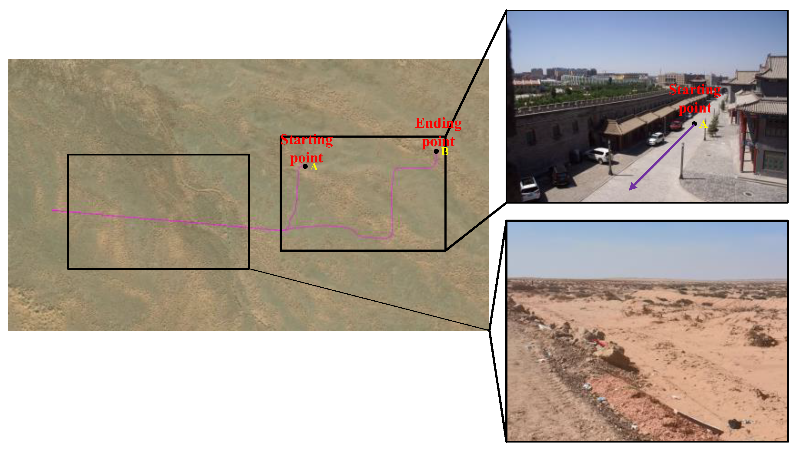
Urban–Gobi Hybrid Environment Localization Experiment

We selected a challenging urban–gobi hybrid environment for comprehensive comparative experiments. The experimental setup in this scenario included Group 1: The proposed adaptive noise filtering fusion method; Group 2: Fixed-noise Error-State Kalman Filter (ESKF-Fixed) fusion algorithm; and Group 3: Differential positioning method based on 4G Qianxun service. This rigorous design thoroughly validates the stability and effectiveness of our method in extreme environments.

4.2. Campus Environment Positioning and Verification Experiment

The campus environment, as a special semi-structured environment, has both structured large buildings or forests that can block signals and sparse areas such as squares or open spaces, posing certain challenges for satellite positioning. This paper selected a closed-loop road section approximately 3 km long within the campus, whose approximate location on the satellite tile map is shown as the red line segment in Figure 9.

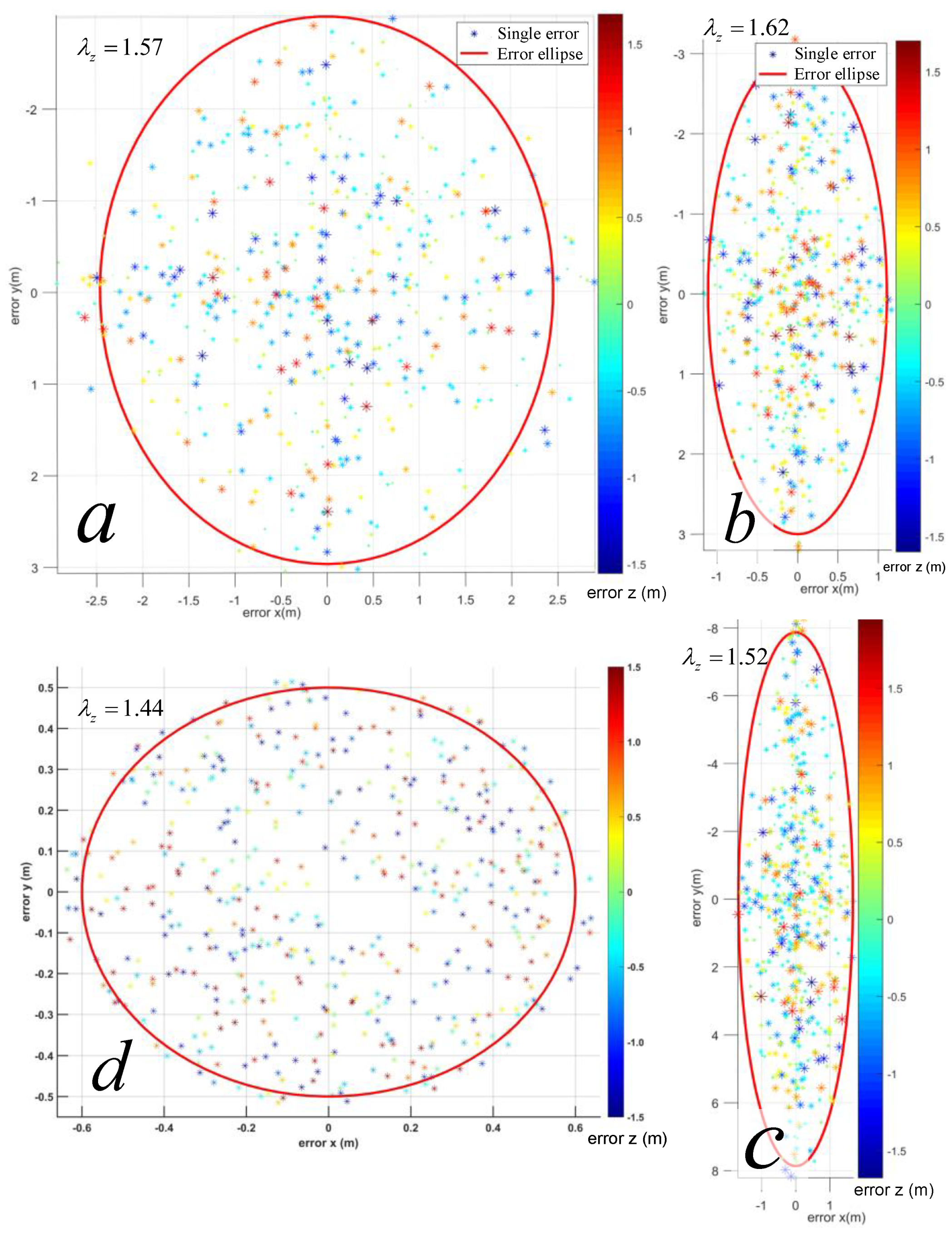
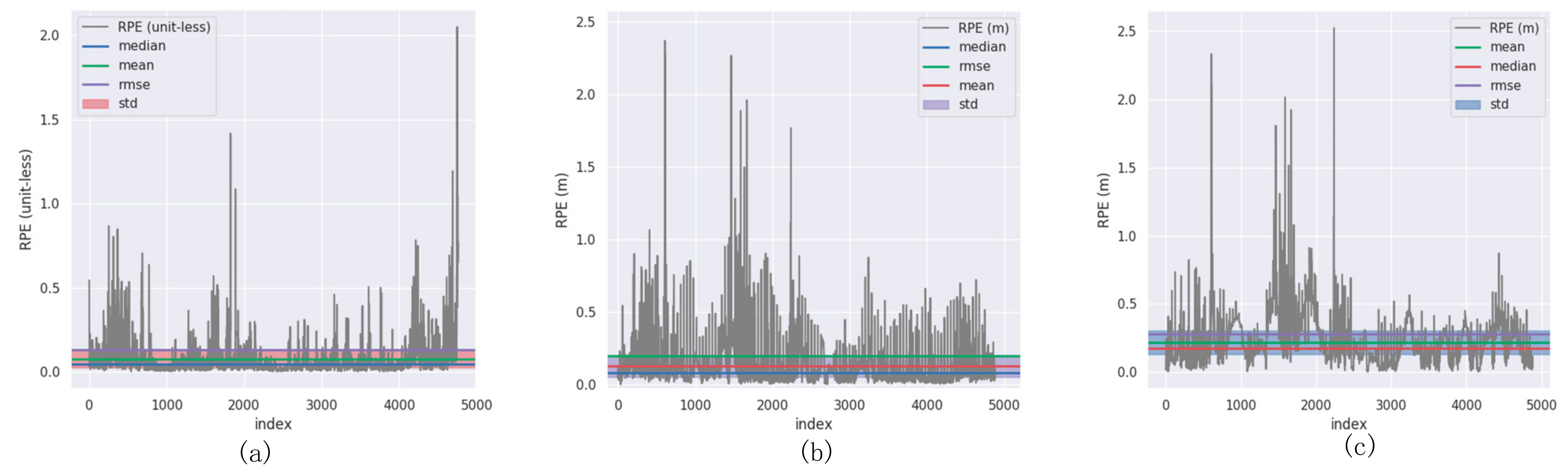
4.2.1. GNSS Positioning Noise Estimation Model Validation Experiment

For the validation of the GNSS positioning noise covariance estimation model, since the model outputs the covariance matrix of position errors (denoted as $\mathrm{cov}\left(\mathsf{\Delta }x\right)$), which characterizes the uncertainty of GNSS-based position estimation across spatial dimensions, an intuitive verification method is required to evaluate its effectiveness. Specifically, as shown in Equation (33), the three eigenvalues of the covariance matrix are utilized as the semi-axis lengths of an ellipsoid in their corresponding directions to geometrically represent the spatial uncertainty of the current positioning solution. The semi-axis lengths of the ellipsoid directly correlate with directional uncertainties: the longer the semi-axis in a particular direction, the greater the uncertainty and the lower the positioning confidence in that direction.

$$\left\{\begin{array}{c}a={\lambda }_x,b={\lambda }_y,c={\lambda }_z\\ {\lambda }_i\in \left\{\lambda |det(cov(\Delta \mathbf{x})-\lambda \mathbf{I})=0\right\},i=x,y,z\end{array}\right.$$

(33)

where ${\lambda }_i$ represents the eigenvalues of the matrix in the x, y, and z directions, and a, b, c represent the semi-axes lengths of the ellipsoid in the x, y, and z directions, respectively.

To validate the satellite positioning noise covariance estimation model, four representative scenarios were selected from the prior constructed map, where 3D LiDAR point clouds were used to more clearly display environmental features in different scenes. The noise covariance ellipsoids derived from the output covariance matrices of the model were mapped onto these scenarios, yielding the local enlarged views (a, b, c, and d) illustrated in Figure 10. Scenario a is situated in an open area behind a classroom building, surrounded by high-rise structures and dense foliage. Owing to severe multipath effects, the noise covariance ellipsoid provided by the estimation model exhibits significant expansion, indicating substantial uncertainties in both longitudinal and lateral positioning. Scenario b corresponds to a right-angled bend with walls obstructing the front and rear sections, while the sides remain relatively unobstructed. The noise covariance ellipsoid demonstrates a smaller lateral radius and a larger longitudinal radius, aligning with the environmental constraints. Scenario c is located at a square in front of a large office building where the vehicle is parked facing away from the building. The estimated noise covariance ellipsoid adopts an elongated shape, reflecting heightened longitudinal uncertainty due to satellite signal blockage by the building, while lateral uncertainty remains minimal. Scenario d represents a crossroads surrounded by low fences and shrubs, offering an unobstructed observation perspective. The compact noise covariance ellipsoid confirms reduced positioning uncertainty under open-sky conditions.

For further quantitative validation of the satellite positioning noise covariance estimation model, this study employed fixed-solution differential GNSS positions as ground truth to calculate the positioning errors of single-point GNSS solutions at specific locations across four scenarios. By repeating satellite observations 500 times at identical locations under varying temporal conditions, the error distribution is plotted in Figure 11, where the color gradient in the right-side bar indicates the magnitude of vertical errors. The covariance matrix generated by the proposed noise estimation model is projected onto Figure 11 to derive a 2D noise covariance ellipse, and the proportion of error points enclosed within the ellipse is statistically analyzed. To benchmark the advancement of our method, the error covariance matrix obtained from the stochastic error estimation model in reference [24] is similarly mapped to the empirical error distribution, generating a 2D covariance ellipse. From Figure 11, it can be clearly seen that the true distribution of single-point positioning errors is in good agreement with the results given by our noise estimation model. The error distribution of the true elevation (i.e., z-axis direction) is between −1.5 m and 1.5 m, which is consistent with the eigenvalue (${\lambda }_z$) of the covariance matrix on the z-axis given by the model. The proportion of positioning errors falling within the ellipse is then calculated for comparative evaluation. The proposed model achieves error coverage rates of 96.6%, 98.2%, 97.8%, and 95.6% across scenarios a, b, c, and d, respectively, with an average coverage rate exceeding 97.05%. In contrast, the method in [24] yields an average coverage rate of 70.5%, indicating that the proposed approach improves the estimation accuracy of GNSS position error covariance by 37.7%. This rigorous validation framework confirms the superior accuracy and environmental adaptability of the proposed noise covariance estimation model, particularly under heterogeneous observation conditions.

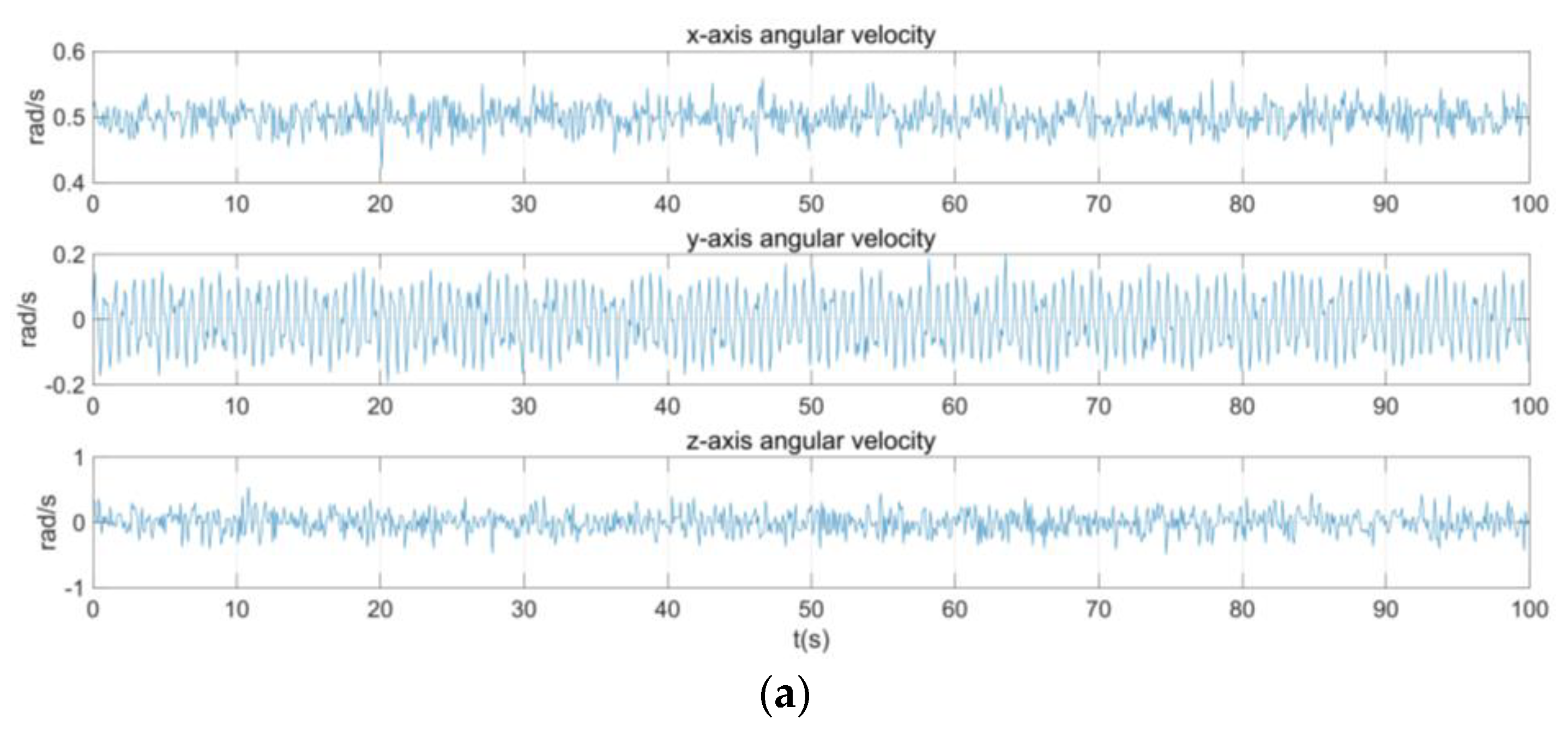
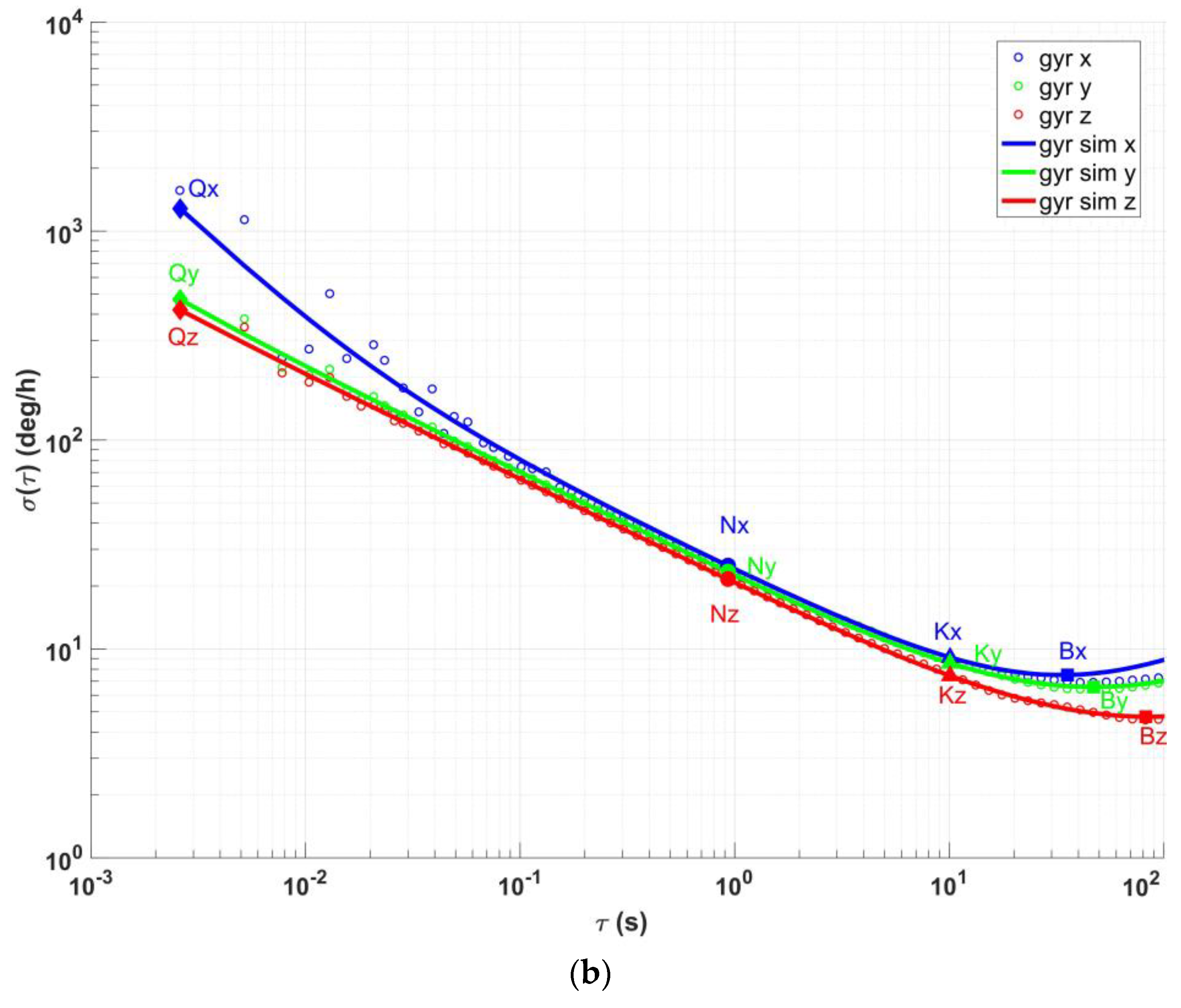
4.2.2. INS Noise Estimation Model Validation Experiment

We collected raw gyroscope output data from a vehicle traveling on an uneven road section in a campus environment to validate our proposed INS noise estimation model. The gyroscope was integrated within an INS550D inertial navigation system. The total data collection duration was 10 min, with a dynamic sliding window length $\mathsf{\Delta }T$ of 100 s. A specific 100 s segment of the collected data was selected for INS noise estimation. After setting the start time of this segment to zero, the raw gyroscope output is shown in Figure 12a. The Allan variance curve obtained after preprocessing the raw data is presented in Figure 12b. From this, we dynamically estimated the values of various INS noise terms, as listed in

Table 2. Various noise values of gyroscope.

Noise Type	X-Axis	Y-Axis	Z-Axis	Unit
Quantization Noise (Q)	1.926	0.708	0.631	$\mathrm{deg}$
Angular Random Walk (N)	24.969	23.344	21.520	$\mathrm{deg}/{\mathrm{h}}^{1/2}$
Angular Rate Random Walk (K)	4.964	4.666	4.059	$\mathrm{deg}/\mathrm{h}$
Bias Instability (B)	7.508	6.576	4.733	$\mathrm{deg}/{\mathrm{h}}^{3/2}$

(the rate ramp was not estimated in this dataset due to the limited sliding window length; it may be re-estimated using multiple historical data segments). The results show that the estimated noise terms closely match the inherent noise characteristics of the gyroscope itself and remain unaffected by disturbances from the uneven road surface and vehicle vibrations. This validates the effectiveness of our proposed INS noise estimation model under dynamic conditions.

4.2.3. Fusion Positioning Comparison Experiment

The positioning comparison experiment was carried out along the red closed-loop road in Figure 9. The positioning values obtained by the error state Kalman filter fusion method (ESKF) based on fixed noise, the adaptive noise filter fusion positioning method, and the VB_AKF method in this paper were compared with the real values of vehicle positioning. The comparison results are as follows:

As illustrated in the trajectory comparison of Figure 13 and Figure 14, the proposed algorithm (red curve) exhibits significantly higher alignment with the ground truth (dashed line) compared to alternative methods. Notably, in the zoomed-in section of the trajectory, GNSS positioning deviations occur due to degraded satellite observation quality caused by surrounding high-rise buildings. The ESKF fusion algorithm with fixed noise parameters (green curve) accumulates positional drift under such conditions and exhibits abrupt jumps upon sudden signal recovery. In contrast, the proposed algorithm dynamically adapts the observation noise covariance of the GNSS module based on real-time measurement quality, maintaining accurate pose estimation throughout. The proposed algorithm achieves an average absolute trajectory error (AATE) of less than 0.6 m, fulfilling the localization requirements for unstructured environments. As summarized in

Table 3. Relative pose error statistical parameters of campus environment.

Method	Maximum Error (m)	Average Error (m)	Root Mean Square (m)	Sum of Variance (m2)
Proposed	2.0472	0.0788	0.1319	82.8566
ESKF-fixed	2.3688	0.1245	0.1955	186.4935
VB_AKF	2.5258	0.2205	0.2809	385.0484

, compared to the fixed-noise ESKF algorithm, the proposed method reduces the maximum relative pose error by 13.58%, the mean relative pose error by 36.71%, the root mean square (RMS) of relative pose error by 32.53%, and the variance of relative pose error by 55.57%. These statistically significant improvements conclusively validate the effectiveness of the adaptive observation noise estimation framework in mitigating GNSS degradation impacts.

To quantify performance, we measured execution times on our experimental platform (representative of current automotive development compute power); the experimental results are shown in

Table 4. Performance of each module during runtime.

Module	Frequency (Hz)	Avg. Time (ms)	Max Time (ms)
GNSS Noise Estimation	10	0.87	1.54
INS Noise Estimation	0.01 (1/100)	15.52	25.28
ESKF Prediction	100	0.05	0.12
ESKF Update	10	0.18	0.33

.

From Table 4, it can be seen that the various modules of fusion positioning have high real-time performance and low computation time on our experimental platform. The core operations of the GNSS noise model involve matrix constructions (O(n)), a small (4 × 4) weighted least-squares inversion (O(3³)), residual calculation (O(n)), and scalar variance estimation (O(1)). The dominant factor is linear in the number of visible satellites n, resulting in very low computational burden (O(n)). Using elevation/azimuth for the geometry matrix H (Equation (10)) avoids complex derivative calculations. The key optimization of the INS noise model is the use of a fixed-length sliding window ($\mathsf{\Delta }T$= 100 s). Calculating Allan variance points (Equation (18)) requires computing differences of group averages over this window. While the window may contain thousands of points (N), the calculation is O(K) ≈ O(N/group_size), effectively O(N) per estimation run. Crucially, this estimation runs at a very low frequency (e.g., 0.01 Hz when $\mathsf{\Delta }T$ = 100 s) in a background thread, not at the IMU rate. Noise parameters are cached and reused for dynamic Q updates. Prediction and update steps of ESKF involve operations on fixed-size matrices (state dim = 15, obs dim = 3). The complexity is O(15³) per step, which is manageable even at high rates (100–200 Hz) on modern embedded processors.

These results demonstrate that the pipeline operates comfortably in real time on our platform, with ample headroom. The latency-critical ESKF steps are extremely fast (sub-millisecond). The heavier INS noise estimation runs infrequently without impacting real-time output.

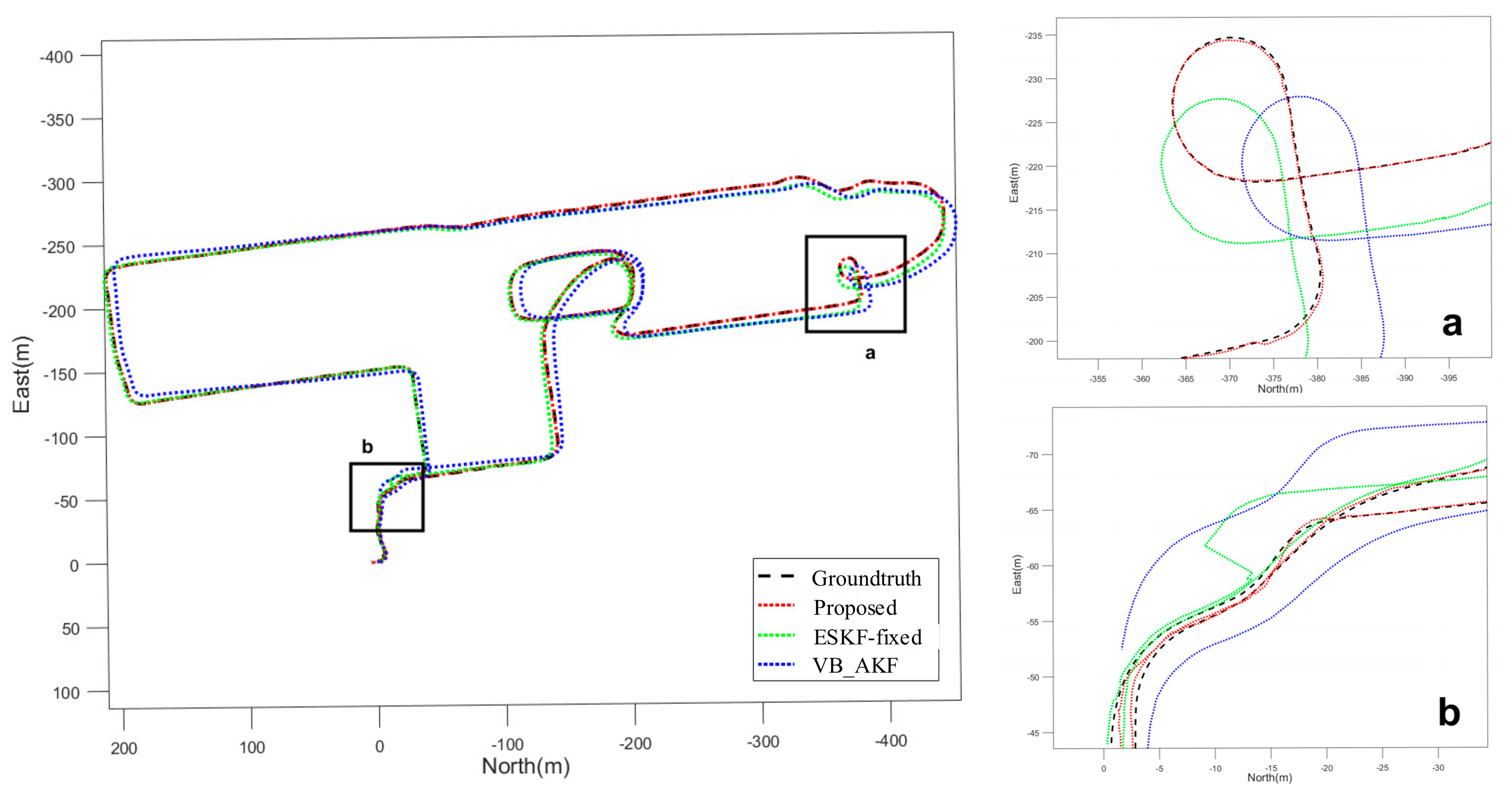
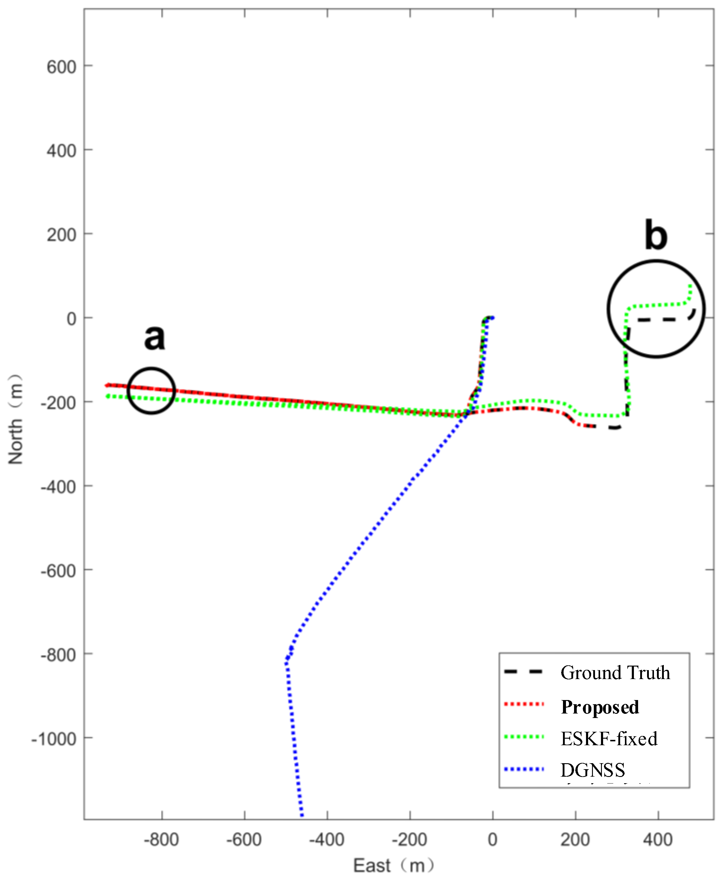
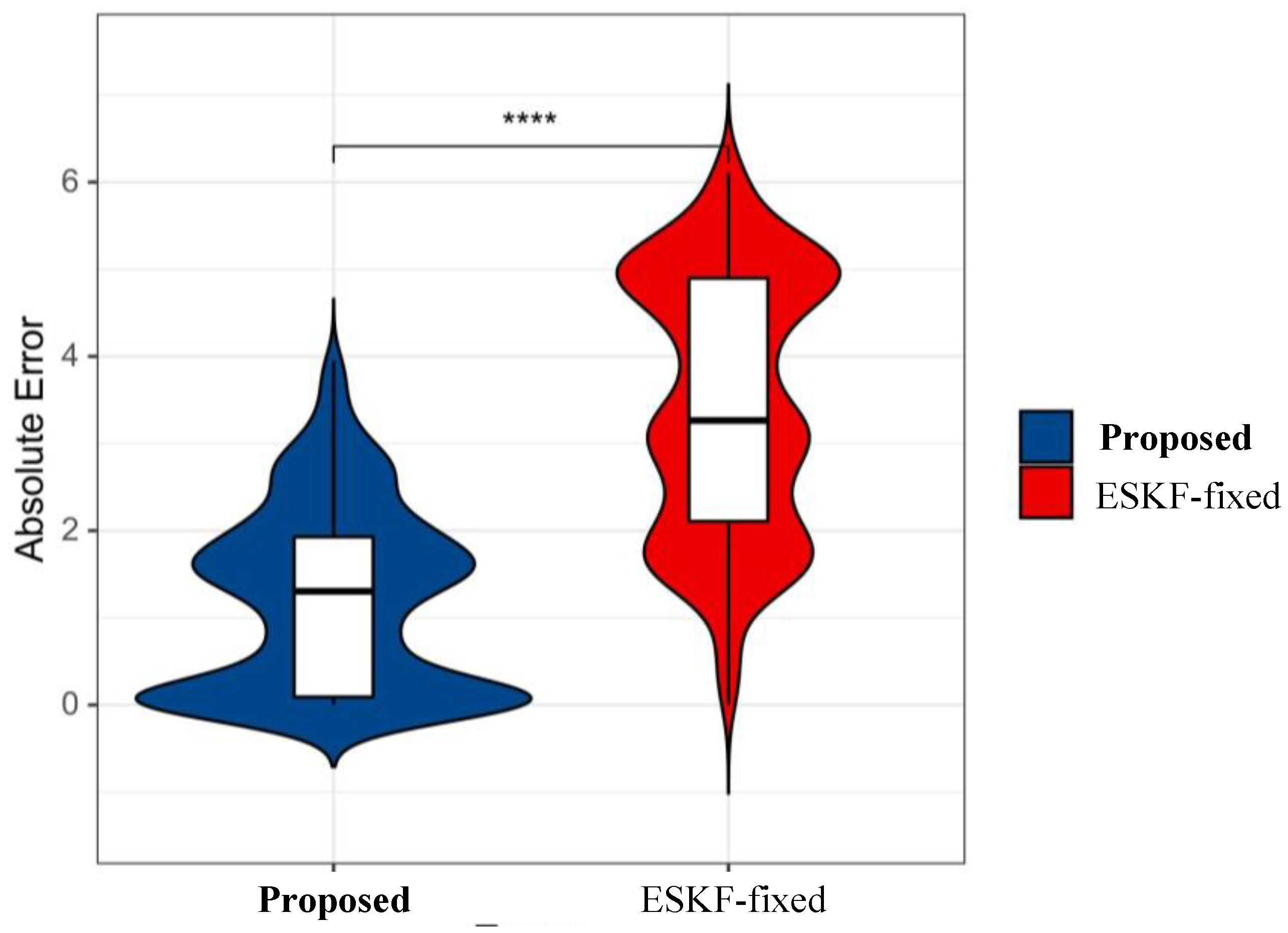
4.3. Comparison of Localization in Urban–Gobi Mixed Environments

We selected the red segment shown in Figure 15 for the fusion positioning experiment. This segment is located in a specific location in Inner Mongolia Autonomous Region, China. It can be observed from the figure that this area consists of an artificially constructed urban simulation environment and vast gobi areas. The experiment starts from an urban scene, passes through a long stretch of gobi road, and then turns around and returns to the urban area via the same route.

The obtained positioning results from the three aforementioned experiments, when compared with the actual vehicle positioning values, yielding the following results:

As demonstrated in the trajectory plot of Figure 16, the GNSS differential positioning method rapidly diverges and fails entirely upon transitioning from the urban environment to the feature-sparse gobi environment. This failure stems from the loss of 4G signal connectivity, which prevents the acquisition of valid differential corrections from the Qianxun service. In contrast, the fixed-error integrated positioning method performs markedly better. However, as positioning duration in the gobi environment increases, its error gradually accumulates due to interference from unreliable satellite positioning results, as illustrated in regions a and b of Figure 16. Notably, the noise estimation-guided integrated positioning method proposed in this study exhibits significantly improved stability and accuracy, remaining robust against satellite signal quality degradation. A comparative analysis of absolute and relative trajectory errors between our method and the fixed-error integrated positioning approach is presented in Figure 17 and

Table 5. Relative pose error statistical parameters of urban–gobi mixed environment.

Method	Maximum Error (m)	Average Error (m)	Root Mean Square (m)	Sum of Variance (m2)
Proposed	0.7310	0.0919	0.1097	11.4267
ESKF-fixed	0.8809	0.1016	0.1240	18.3227

.

As evidenced by the results in Figure 17 and Table 5, the noise estimation model-guided integrated positioning method proposed in this study achieves significantly lower absolute trajectory errors compared to the fixed-error integrated positioning method, with reduced error fluctuation ranges. The mean absolute trajectory error is less than 1.2 m, substantially outperforming the precision level of standalone sensors. Based on the statistical parameters of relative pose errors calculated in Table 2, our method exhibits reductions of 17.02% in maximum relative pose error and 9.55% in average relative pose error over the fixed-error integrated positioning approach (ESKF-fixed). Furthermore, the root mean square (RMS) and variance values of relative pose errors decrease by 11.53% and 37.64%, respectively. These metrics thoroughly validate the robustness of the proposed algorithm in extreme operational environments.

5. Conclusions

We proposed a noise-adaptive GNSS/INS fusion framework to address the challenges of dynamic sensor reliability in complex environments for autonomous driving. By integrating dual noise estimation models—combining satellite elevation/SNR-based a priori weighting with Helmert posterior variance estimation for the GNSS, and Allan variance-driven INS bias instability modeling—the framework dynamically adjusts process and observation noise covariances in an Error-State Kalman Filter (ESKF). Experimental results demonstrated significant advancements: The GNSS noise estimation model achieved 37.7% higher accuracy in uncertainty quantification compared to elevation-only methods, effectively mitigating multipath and ionospheric errors. The fusion system maintained an average absolute trajectory error (ATE) < 0.6 m in unstructured environments, outperforming the fixed-weight ESKF by 36.71% in positioning consistency.

This research bridges the gap between theoretical noise modeling and real-world adaptability, offering a robust solution for autonomous systems operating in GNSS-degraded scenarios. Future research will extend the framework to incorporate LiDAR/vision modalities and optimize computational efficiency for edge deployment.

References

1. Wang, E.; He, H.; Jia, C. Evaluation Methods of Satellite Navigation System Performance; IntechOpen: London, UK, 2019. [Google Scholar] [CrossRef]
2. Zhen, W.; Zeng, S.; Soberer, S. Robust localization and localizability estimation with a rotating laser scanner. In Proceedings of the 2017 IEEE International Conference on Robotics and Automation (ICRA), Singapore, 29 May–3 June 2017; pp. 6240–6245. [Google Scholar]
3. Li, X.; Chen, L.; Lu, Z.; Wang, F.; Liu, W.; Xiao, W.; Liu, P. Overview of Jamming Technology for Satellite Navigation. Machines 2023, 11, 768. [Google Scholar] [CrossRef]
4. Tan, H.S.; Huang, J. DGPS-Based Vehicle-to-Vehicle Cooperative Collision Warning: Engineering Feasibility Viewpoints. IEEE Trans. Intell. Transp. Syst. 2006, 7, 415–428. [Google Scholar] [CrossRef]
5. Qin, C.; Ye, H.; Pranata, C.E.; Han, J.; Zhang, S.; Liu, M. R-lins: A robocentric LiDAR-inertial state estimator for robust and efficient navigation. arXiv 2019, arXiv:1907.02233. [Google Scholar]
6. Xing, Z.; Xia, Y. Multi-sensor optimal distributed weighted Kalman filter fusion over unreliable networks. In Proceedings of the 2016 35th Chinese Control Conference (CCC), Chengdu, China; 2016; pp. 4926–4931. [Google Scholar] [CrossRef]
7. Jiang, C.; Wang, Z.; Liang, H.; Zhang, S.; Tan, S. Motion State Estimation Based on Multi-sensor Fusion and Noise Covariance Estimation. Proceedings of 2021 International Conference on Autonomous Unmanned Systems (ICAUS 2021). ICAUS 2021; Wu, M., Niu, Y., Gu, M., Cheng, J., Eds.; Lecture Notes in Electrical Engineering. Springer: Singapore, 2022; Volume 861. [Google Scholar] [CrossRef]
8. Gu, T.; Chen, S.; Tan, J.; Wang, C.; Chen, A. Research on Multi source Integrated Navigation Algorithm of SINS/GNSS/OD/Altimeter Based on Federated Filtering. Navig. Position. Timing 2021, 8, 20–26. [Google Scholar] [CrossRef]
9. Shan, T.; Englot, B.; Meyers, D.; Wang, W.; Ratti, C.; Rus, D. LIO-SAM: Tightly-coupled Lidar Inertial Odometry via Smoothing and Mapping. In Proceedings of the 2020 IEEE/RSJ International Conference on Intelligent Robots and Systems (IROS), Las Vegas, NV, USA, 24 October–24 January 2020; pp. 5135–5142. [Google Scholar] [CrossRef]
10. Ye, H.; Chen, Y.; Liu, M. Tightly Coupled 3D Lidar Inertial Odometry and Mapping. In Proceedings of the 2019 International Conference on Robotics and Automation (ICRA), Montreal, QC, Canada, 20–24 May 2019; pp. 3144–3150. [Google Scholar] [CrossRef]
11. Shan, T.; Englot, B.; Ratti, C.; Rus, D. LVI-SAM: Tightly-coupled LiDAR-Visual-Inertial Odometry via Smoothing and Mapping. arXiv 2021, arXiv:2104.10831. [Google Scholar]
12. Huang, Z.; Chai, H.; Xiang, M.; Du, Z. AUV multi-source information fusion localization method based on robust factor graph. Acta Geod. Cartogr. Sin. 2023, 52, 1278–1285. [Google Scholar] [CrossRef]
13. Gao, X.; Chen, J.; Tao, D.; Li, X. Multi-Sensor Centralized Fusion without Measurement Noise Covariance by Variational Bayesian Approximation. IEEE Trans. Aerosp. Electron. Syst. 2011, 47, 718–772. [Google Scholar] [CrossRef]
14. Wang, D.; Zhang, H.; Ge, B. Adaptive Unscented Kalman Filter for Target Tacking with Time-Varying Noise Covariance Based on Multi-Sensor Information Fusion. Sensors 2021, 21, 5808. [Google Scholar] [CrossRef] [PubMed]
15. Duník, J.; Kost, O.; Straka, O. Design of measurement difference autocovariance method for estimation of process and measurement noise covariances. Automatica 2018, 90, 16–24. [Google Scholar] [CrossRef]
16. Gao, Z.; Zhong, Y.; Zong, H.; Gao, G. Adaptive Random Weighted H∞ Estimation for System Noise Statistics. Int. J. Adapt. Control. Signal Process. 2025, 39, 214–230. [Google Scholar] [CrossRef]
17. Gao, Z.; Zong, H.; Zhong, Y.; Gao, G. Limited Memory-Based Random-Weighted Kalman Filter. Sensors 2024, 24, 3850. [Google Scholar] [CrossRef] [PubMed]
18. Hu, J.; Wang, Y.; Yan, Y.; Ren, Y.; Wang, Y.; Yin, G. Estimation of Vehicle State Based on Limited Memory Random Weighted Unscented Kalman Filter. In Proceedings of the 2021 5th CAA International Conference on Vehicular Control and Intelligence (CVCI), Tianjin, China, 29–31 October 2021; pp. 1–6. [Google Scholar] [CrossRef]
19. Gao, Z.; Mu, D.; Gao, S.; Zhong, Y.; Gu, C. Adaptive unscented Kalman filter based on maximum posterior and random weighting. Aerosp. Sci. Technol. Vol. 2017, 71, 12–24. [Google Scholar] [CrossRef]
20. Gao, S.; Hu, G.; Zhong, Y. Windowing and random weighting-based adaptive unscented Kalman filter. Int. J. Adapt. Control. Signal Process. 2015, 29, 201–223. [Google Scholar] [CrossRef]
21. Hu, G.; Gao, B.; Zhong, Y.; Gu, C. Unscented kalman filter with process noise covariance estimation for vehicular ins/gps integration system. Inf. Fusion 2020, 64, 194–204. [Google Scholar] [CrossRef]
22. Gao, B.; Gao, S.; Hu, G.; Zhong, Y.; Gu, C. Maximum likelihood principle and moving horizon estimation based adaptive unscented Kalman filter. Aerosp. Sci. Technol. 2018, 73, 184–196. [Google Scholar] [CrossRef]
23. Duan, S.; Sun, W.; Wu, Z. Application of robust adaptive EKFin INS/GNSStight combination. J. Univ. Electron. Sci. Technol. China 2019, 48, 216–220. [Google Scholar] [CrossRef]
24. Yang, L.; Lin, X.; Hou, Y.; Ren, J.; Wang, M. Application of an Improved Adaptive Unscented Kalman Filter in Vehicle Driving State Parameter Estimation. Int. J. Adapt. Control. Signal Process. 2025, 39, 1021–1035. [Google Scholar] [CrossRef]
25. Feng, B.; Fu, M.; Ma, H.; Xia, Y.; Wang, B. Kalman Filter with Recursive Covariance Estimation—Sequentially Estimating Process Noise Covariance. IEEE Trans. Ind. Electron. 2014, 61, 6253–6263. [Google Scholar] [CrossRef]
26. Narasimhappa, M.; Mahindrakar, A.D.; Guizilini, V.C.; Terra, M.H.; Sabat, S.L. MEMS-Based IMU Drift Minimization: Sage Husa Adaptive Robust Kalman Filtering. IEEE Sens. J. 2020, 20, 250–260. [Google Scholar] [CrossRef]
27. Zhou, G.; Du, Z.; Xie, L.; Wang, T.; Liu, X. Attitude calculation based on Allan variance adaptive algorithm. Ordnance Autom. 2018, 37, 32–36. (In Chinese) [Google Scholar] [CrossRef]
28. Shang, M.; Gao, H.; Chang, Q.; Xu, Y.; Wu, J.; Zhang, J. Weighting Method for GPS/GLONASS/BDS Three System Integrated Positioning. J. Terahertz Sci. Electron. Inf. 2014, 3, 374–379. (in Chinese). [Google Scholar] [CrossRef]
29. Ma, Q. Research on Differential Estimation of GPS/BDS/DORIS/SLR Observation Noise. Master’s Thesis, China University of Mining and Technology, Xuzhou, China, 2016. (In Chinese). [Google Scholar]
30. Brossard, M.; Barrau, A.; Bonnabel, S. AI-IMU dead-reckoning. IEEE Trans. Intell. Veh. 2020, 5, 585–595. [Google Scholar] [CrossRef]
31. Li, Y.; Huang, D.; Li, M.; Zhu, D. BDS/GPS Stochastic Model Refinement and Assessment Using Satellite Elevation Angle and SNR. In China Satellite Navigation Conference (CSNC) 2015 Proceedings: Volume I; Lecture Notes in Electrical Engineering; Sun, J., Liu, J., Fan, S., Lu, X., Eds.; Springer: Berlin/Heidelberg, Germany, 2015; Volume 340. [Google Scholar] [CrossRef]
32. Lemmon, T.R.; Gerdan, G.P. The Influence of the Number of Satellites on the Accuracy of RTK GPS Positions. Aust. Surv. 1999, 44, 64–70. [Google Scholar] [CrossRef]
33. Bilich, A.; Larson, K.M. Mapping the GPS multipath environment using the signal-to-noise ratio (SNR). Radio Sci. 2007, 42, 42–58. [Google Scholar] [CrossRef]
34. Brian, E.G.; Mark, A.B. A Least-Squares Normalized Error Regression Algorithm with Application to the Allan Variance Noise Analysis Method. In Proceedings of the 2006 IEEE/ION Position, Location, And Navigation Symposium, Coronado, CA, USA, 25–27 April 2006. [Google Scholar] [CrossRef]
Figure 1. Schematic diagram of multi-sensor fusion positioning.
Vehicles 07 00077 g001
Figure 2. An overview of the proposed adaptive noise fusion localization framework.
Vehicles 07 00077 g002
Figure 3. Schematic diagram of satellite positioning principle.
Vehicles 07 00077 g003
Figure 4. Flowchart of the satellite positioning estimation algorithm.
Vehicles 07 00077 g004
Figure 5. Schematic diagram of the variance versus time interval log–log curve.
Vehicles 07 00077 g005
Figure 6. A schematic diagram of obtaining vehicle localization status through dynamic noise estimation and ESKF fusion.
Vehicles 07 00077 g006
Figure 7. Noise adaptive ESKF fusion flowchart.
Vehicles 07 00077 g007
Figure 8. Real vehicle validation platform.
Vehicles 07 00077 g008
Figure 9. Campus validation environment satellite cloud map.
Vehicles 07 00077 g009
Figure 10. Special scene error ellipsoid display. In the figure (ad) represent the four different scenarios in the campus environment, and the red ellipsoid represents the visualization of the noise covariance matrix output by the GNSS noise estimation model, while the colored scatter points represent the real-time point cloud of the surrounding environment.
Vehicles 07 00077 g010
Figure 11. Comparison diagram of multiple single-point positioning error distribution and estimated covariance ellipse. In the figure (ad) represent the four different scenarios corresponding to Figure 10. The red ellipse represents the two-dimensional projection of the error covariance matrix given by our proposed GNSS noise estimation model on the x-y plane. The “*” shaped scatter points represent the error distribution of 500 single-point positioning operations in the corresponding scenario. The color of the scatter points corresponds to the color mapping bar on the right, representing the error distribution of elevation (z-axis).
Vehicles 07 00077 g011
Figure 12. Allan variance estimation of gyroscope. (a) Gyroscope raw output; (b) Allan variance log–log curve.
Vehicles 07 00077 g012aVehicles 07 00077 g012b
Figure 13. Comparison diagram of experimental track of campus environment positioning. In the figure, a marks a location with severe satellite signal obstruction, where the vehicle also performed a steering maneuver; b is near the endpoint of the entire route and also experiences tree obstruction.
Vehicles 07 00077 g013
Figure 14. Comparison diagram of relative pose errors. (a) The proposed approach; (b) ESKF-fixed method; (c) VB_AKF method.
Vehicles 07 00077 g014
Figure 15. Urban–gobi mixed environment satellite cloud map.
Vehicles 07 00077 g015
Figure 16. Trajectory comparison diagram in urban−gobi mixed environment. In the figure, a marks a location deep in the Gobi Desert where 4G differential service is unavailable; b indicates a location in an urban environment that is blocked by buildings.
Vehicles 07 00077 g016
Figure 17. Absolute trajectory error comparison chart. In the figure, “****” represents the degree of correlation between data, with the highest being “*****”.
Vehicles 07 00077 g017