Abstract
Railways are complex systems, and the braking performance of trains is crucial to ensure the line’s safety. The assessment of the stopping distance can be obtained by empirical formulas or by more sophisticated numerical models which simulate the train’s longitudinal dynamics. In both cases the level of estimation accuracy may vary a lot, depending on the numerical values attributed to several parameters related both to the train braking system and the railway. The correct identification of such parameters might be an issue in local railways. On the one hand, some widely used empirical formulas are mainly intended for national railways, thus it is critical to determine whether they are appropriate for local railways. On the other hand, the development of a good predictive simulation model requires the identification of parameters not always known for the trains in service. Starting with measurements taken from braking tests performed on a local railway, this research aims to propose an experimentally correlated dynamics model based on the train’s equation of motion that can accurately estimate the stopping distance with a reduced amount of input parameters obtainable from measurements. Several braking tests have been performed on the track to identify the model’s parameters and to enhance the numerical–experimental correlation. Meanwhile, the applicability of stopping distance empirical formulas to the case of local railways has been evaluated, and the parameters of these formulas have been identified to reduce the gap with respect to measured distance values. Even if both simulation approaches led to an accurate estimation of the stopping distance, this work highlights some distinctions. In order to match the measured distance values, some empirical formulas required the definition of doubtful input parameters values, and suggest skipping their use for local railways application. Conversely, the proposed dynamics model led to a good balance between accuracy level and the effort required for parameter identification from testing, with it being more easily applicable to different scenarios and open to the implementation of additional features in future studies.
1. Introduction
The use of predetermined tracks makes rail transportation one of the safest modes, especially compared to road traffic. However, the technical complexity of railways, the interaction with surroundings, and the high number of passengers make safety a primary concern [1,2]. The level of safety is determined by many factors [3], which includes the braking performances of the trains and their capability to stop within a certain distance to safely plan their travel on the railway [4,5].
The brake stopping distance has a significant impact on the design of block sections, the signalling plan, and overlaps, as well as being included in risk assessments at level crossings. Accidents and fatalities at level crossings account for more than a quarter of all rail accidents on EU railways [1,2], with nearly 300 people dying each year and economic damage estimated at EUR 1 billion. A more accurate prediction of the brake stopping distance in an emergency at a level crossing is fundamental to improve safety in the particular case of local railways [6]. These networks, also known as isolated railways, cover the demand for short- or medium-haul trips, as well as historical and tourist purposes, and operate in heterogeneous environments where traditional trains struggle to run. Over time, due to the different management methodologies, local railways have developed distinctive characteristics and safety standards compared to national railways, hindering the transfer of commonly used management practices and tools. The applicability of risk management models is reduced in such railways systems, where accident data collection has been implemented only recently. The changes introduced in 2019 by the Italian Railway Safety Agency (ANSFISA, formerly ANSF), with input from the European Union Agency for Railways (ERA), pushed for alignment of the safety and quality standards of Italian local railways with the rest of the national railway system [7]. Local railways ask for specific actions to determine the proper risk management models. The braking efficiency and stopping distance, especially in emergency situations at level crossings or when evaluating collision hazards, give fundamental contributions to the risk assessment process, and the availability of a robust calculation method of the braking phase has become an indispensable tool for local railways management.
Various computation models for train stopping distances have been developed over the years, including old but still widely used empirical formulas (i.e., Maison, Pedeluck, and Minden formulas) [5,8,9]. The latter implies the definition of a parameters set that tries to balance the need for general applicability with an acceptable level of accuracy and reliability. These formulas have been developed for railways, primarily national ones, which have characteristics—in terms of horizontal geometry, vertical geometry, and transit speed—that are greatly different from those of local railways.
Besides the mentioned empirical formulas, the scientific literature offers several methodologies to define numerical models to simulate the train’s longitudinal dynamics in the braking phase [10,11,12]. These dynamics models may or may not include a detailed representation of the braking system [13,14] and its components designed to apply brake moments to the train’s wheels, such as devices and pipes for air pressurization [15], brake pads [14,16,17,18], and electro-magnetic systems. The braking force effectively generated at each wheel–rail contact can be estimated through more complex non-linear models based on creepage percentage [19,20,21], or simplified models based on the limitation of longitudinal force when the peak of grip coefficient is reached at large creepage [22,23,24]. Within a so vast scientific application field, some authors have oriented their works more to the braking systems and their components, such as the pads, and others to the wheel–rail interaction, analyzing the different factors governing the generation of the longitudinal braking force, such as the dependency of friction on rail condition—dry, wet, moist, snow, or contaminated [19,25,26]—or effect of train speed and creepage [27].
The current work aims to develop a braking calculation tool—based on the numerical integration of the non-linear longitudinal dynamics equation—which can be easily applied to the considered local railways, taking into account the characteristics of the trains circulating on this line, their braking system, and the peculiarities of the route. As illustrated in the next sections, the development of this model has been performed by writing and solving a set of non-linear equations formulated on the basis of fundamental dynamics principle and by selecting the most useful formulas from different authors. The model creation has been driven by the need to minimize the number of input parameters required to reach an acceptable accuracy level, so as to minimize the effort for their experimental identification. Different brake tests have been performed on the track to identify such model parameters, obtaining a very good correlation between simulation outputs and measured data. Finally, the results obtained from this dynamics model have been compared to those obtained from traditional empirical formulas in order to evaluate their applicability to the context of local railways, and the underlying pros and cons of the two different calculation methods.
2. Brake Stopping Distance of a Train: Definition and Calculation Methods
The brake stopping distance is defined as the distance travelled from the time at which the driver detects an impediment or a signal, and he is going to apply the brakes, until the train comes to a complete stop. An adequate distance is fundamental to guarantee safety during standard or emergency braking operations. The stopping distance depends on several factors, such as:
- The initial speed of the train at the time when the driver decides to actuate the brakes;
- The brake delay time, which is the time required by the brake system to deliver the brake torque at wheels after receiving a given braking demand by the driver;
- The achievable longitudinal deceleration, which varies over time and depends on the amount of brake demand, the nominal characteristics of the train’s brake system, the mass of the train, the slope of the track, and the adhesion in the wheel–rail contact;
- Environmental factors that determine the maximum adhesion coefficient and how it changes with train speed, such as the presence of water, snow, or other contaminants on the tracks;
- The current status of the braking system, including the wear of the brake pads and in the case of hydraulic brakes the effective air pressure in the brake cylinders.
The aim of obtaining an accurate estimation by a calculation model might be challenging due to the high number of non-linear contributions and a moderate degree of uncertainty.
Aside from the calculation method, the train stopping distance in metres, Ls, could be conveniently expressed through the well-known expression [5], which sums two terms as follows:
where Lr [m] is the reaction distance and Lb [m] is the braking distance until stop. From now on, the unit of measure of quantities in formulas will be indicated between square brackets.
The first term is the distance travelled by the train during the time needed by the driver to react to an input (signal, hazard, etc.) and apply the brakes. The train’s speed is assumed to be constant while the reaction distance is travelled, hence its kinematics formula is:
where tr [s] is the driver’s reaction time, v [m/s] is the train initial speed, and vkph is the speed in [km/h], which is the unit mostly used in empirical formulas, as later shown.
In a more general way, the reaction time could also include the braking delay time, which is the time taken by the brake system to deliver the requested braking action after the driver’s action occurs. This approach is typically adopted when simplified or empirical formula are used, and the formula computes only the Lb term.
If a more detailed calculation method is adopted, it is recommended to separate the two delay contributions as they are determined by different causes. They are either subjective and more sensitive to statistical variability, such as the contribution of the driver; or objective and less variable, such as the brake delay time, which is strictly dependent on the brake system type and performance.
If the brake delay time is included in the reaction time, the braking distance is the distance travelled by the train from the time the brake force is fully delivered at the wheel–rail contact until the vehicle comes to a complete stop. If not, the braking distance is the distance travelled by the train from the time at which the brake demand is applied until the vehicle comes to a complete stop.
2.1. Empirical Formulas for Stopping Distance Calculation
In the literature there are several formulas that allow us to determine the stopping distance of a train in an empirical way [5,8,9]. Some of these are conceived in a more general way, whilst others explicitly refer to a type of train (freight or passenger) or are provided for a certain speed range. In this section we present a review of four formulas to show some of their pros and cons. These formulas are:
- Maison formula;
- Pedeluck formula;
- Minden formula;
- Italian formula C.M. 26.
The Maison formula was developed for freight trains with speeds lower than 70 km/h and it is expressed as follows:
beside vkph, which is the already defined initial speed in [km/h], the other parameters are:
- i‰, the track gradient [‰ or mm/m], positive uphill and negative downhill; Equation (3) has been written with an opposite sign applied to i with respect to the original formula to keep the same sign convention for track gradient in the whole manuscript;
- f, the friction coefficient which is assumed to be dependent on the track gradient; suggested values are: f = 0.10 for an absolute value of i < 15‰, andf = 0.10 + 0.00133 (i −15) for an absolute value of i > 15‰;
- λ%, the braking percentage [%], defined as the ratio of the braking force required for braking 1 metric ton to the total vehicle weight; suggested values from literature are reported in Table 1.
 Table 1. Values of λ% for different rolling stocks and braking actions according to [8].
The Pedeluck formula is available in two versions. The first one is defined for passenger trains and speeds between 70 and 140 km/h, and is as follows:
where the parameters are the same of expression (3).
The second version of Pedeluck formula is defined for diesel–electric passenger trains, and the braking distance is given by:
where the new parameter γ [m/s2] is the absolute value of the train deceleration.
Previous formulas, developed by the French railways, are also in use by the International Union of railways (UIC), while another formula used on German railways is the so-called Minden formula [8,9]. Even this one is available in two versions, one for passenger trains (6) and the other for freight trains (7), and they are as follows:
where the adimensional parameter ψ has been introduced to account for the characteristics of the brake system, taking values between 0.5 and 1.25. The braking percentage is still dependant on the rolling stock type, and proposed values are λ% = 40% for freight trains, λ% = 138% for rail vehicles with disc brakes, and λ% = 239% for intercity trains with disc brakes. The braking percentage plays a crucial role in the correct calculation of the braking distance and its value needs to be experimentally identified as well as parameter ψ.
Still used for calculations of braking distance in some local Italian railways, the following formula provided by the Italian “Circolare Ministeriale” (Ministerial Circular) n. 26 of 1971 is given in its original formulation:
where the value suggested for the friction coefficient is f = 0.157. In order to include the dependence of braking distance on rail condition, the formula has been later modified by introducing an additional parameter u (u = 1 dry rail, u = 1.2 intermediate grip, u = 1.6 wet rail) and the track gradient, thus determining the final version as:
All the above empirical formulas come from the general equation of motion in longitudinal direction with the simplification that only brake force, rolling resistance forces, and the weight component generated by the track gradient are applied. This is represented as follows:
where M [kg] is the total mass of the rolling stock, g is the gravity constant (=9.81 m/s2), r is the rolling resistance coefficient, Fb [N] is the sum of all braking forces at wheel rail contacts, i‰ is the already defined track gradient (>0 uphill), and [m/s2] is the train acceleration. [kg] is the sum of the total mass and the equivalent mass determined by the inertia moments of the rotating parts (wheels and other parts) that must be decelerated. The exact calculation requires detailed information on mechanical parts, while an easier estimation could be obtained through the adimensional coefficient β as follows:
Equations (10) and (11) lead to the next more general formula of the braking distance:
The advantage of using one of the empirical formulas instead of (12) is the reduction in parameters to be entered and identified for calculation.
2.2. The Proposed Dynamics Model for Braking Simulation
The dynamics model developed in this work is based on the differential motion equation reported below with non-linear forces depending on the state variable v, which is the train velocity in [m/s]:
The total resistance force R [N] is the sum of the weight component generated by the track inclination, the wheel rolling resistance, and the aerodynamic drag, which is shown as follows:
Equation (14) sums the resistance due to track gradient with the standard Davis equation, so that A coefficient is related to the rolling resistance constant term, B coefficient is related to the mechanical losses, and C coefficient is related to the aerodynamics drag [28,29,30]. A, B, and C can be experimentally determined in a coasting test at null track gradient.
The calculation of the total braking force, Fb, has been performed through a Matlab R2025a user-written function which takes into account the mechanical properties of the braking system and the brake delay time. The friction coefficient between the wheel rail and each brake cast-iron shoe has been expressed as a function of the train velocity and the pressure ppad [bar] transferred to the pads by the hydraulic brake cylinder, both varying with time. The following function has been taken from [13], slightly changed to account for the different unit of measure of pressure, and provided with the scaling factor :
The pressure delivered at the brake pads depends on the pressure reached in the brake cylinder of each bogie unit and the time delay in the hydraulic system [13,14,15]. In order to simplify the representation of delays, following a suggestion in [14], the pressure on the pads is assumed to be instantaneously coincident with the pressure in the brake cylinder and a unique delay is introduced in the expression of the brake cylinder pressure, pbc, which is obtained by the maximum pressure in the brake cylinder, pbcmax, multiplied by the brake demand requested by the driver, % brake command [0–100%], and the delay function Y(t), resulting in the following:
As shown in Figure 1, the Y(t) step function has been implemented in Matlab by a fifth-order polynomial, defined through the start time, tS [s], at which the function is still null, and the end time, tE [s], at which it achieves 1. The two parameters could be estimated by measuring both the brake command and the cylinder pressure to obtain the time at which 95% of steady-state pressure is reached.

Figure 1.
Time function Y(t) which models the delay in the growth of the braking pressure and force.
The total braking force can be obtained by the next expression, which has been formulated by simplifying the corresponding equation used in [13]:
where a constant gain kp [N/bar] has been introduced to account for the characteristics of the braking system. This approach has been used in this work to simplify the original formula and use a unique coefficient which is easier to be experimentally determined.
Following a simplified approach that uses a maximum adhesion coefficient at large creepage, the total braking force is limited by the adhesion at wheel to rail contact, being the limit force value given by the next equation:
where P [N] is the sum of forces normal to the rail path, and is the maximum adhesion coefficient depending on train velocity.
There are several friction models available from the literature and most of them have been reviewed in [22]. In order to reduce the number of parameters to be identified, only those rational models reported in Table 2 have been introduced in the dynamics model. They range from old models, like the Bochet’s one, to more recent versions used in several railway systems for longitudinal dynamics calculations. The values of the maximum adhesion coefficient at zero speed and at 50 km/h have been reported in Table 2 for different rail conditions. In particular, at 50 km/h, which is the maximum speed in the analyzed local railway, values for dry contact range from 0.15 to 0.26.
Table 2.
Maximum adhesion coefficient at wheel–rail contact depending on train speed.
The plot of the adhesion coefficient versus speed for the above-listed rational models is shown in Figure 2 for dry condition only. While the friction model n.4 saturates above 30 km/h, all other models show comparable behaviours.
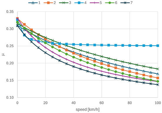
Figure 2.
Changes in maximum adhesion coefficient with train’s speed in dry track conditions using rational models reported in Table 2.
The numerical integration in Matlab of the non-linear differential Equation (13), starting from the initial speed of the train, allows one to determine the time histories of the different quantities, such as pressure in the master cylinder, deceleration, speed, and distance travelled, thus calculating the distance travelled to reach an assigned lower speed or the distance Ls at stop. In this case, the driver reaction time of Equation (2) could be eventually included in the Y(t) function as an extended start time at zero pressure.
In the proposed dynamics model, the equations selected from the literature have been modified in an attempt to reach a good balance between accuracy level and effort for parameters identification from testing. This makes them more easily applicable to different scenarios and open to the implementation of modified or additional features in future studies.
3. The Testing Activities and the Measured Signals
The experimental braking tests have been performed on a local railway located in Sicily on the Etna Volcano, with an old ADE 19 diesel electric railcar built in 1974, equipped with two bogies and two driving cabs located at both ends. The measured running mass was 31.9 [ton]. The braking system has a modulable pressure cylinder that delivers pressure to separate cylinders in the two bogies. The pressure at each bogie’s cylinder is transferred through pipes to cast-iron shoes providing braking action to the 4 wheels of the bogie, having a radius of 0.375 [m] and a moment of inertia of 1 [kg·m2]. Figure 3 shows the railway vehicle used for the tests and the driver’s cab with the acquisition system installed.
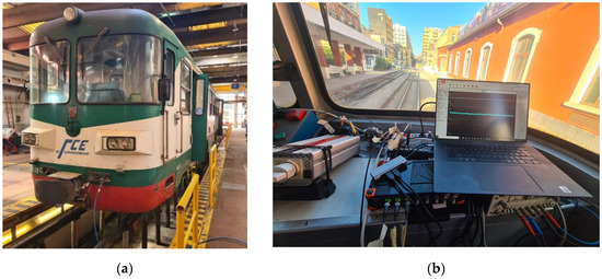
Figure 3.
The rail vehicle used in brake tests: (a) front view; (b) view from the driver’s cabin and installed DEWEsoft acquisition systems.
The setup of the instrumentation devices to estimate the braking performance of the rail vehicle included:
- One high-gain GPS antenna—Sauchy Data System xPro Nano (Figure 4a)—with inertial measurement unit (IMU) using digital communication to send measured data through the CAN bus;
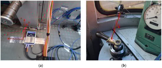 Figure 4. Installed instrumentation devices: (a) the xPro Nano system with IMU mounted on the floor with the X-axis along the train motion direction and the Z-axis pointing up; and (b) the wire potentiometer used to measure the position of the braking lever command actuated by the driver.
 - Three analogue pressure sensors to measure pressure at the master cylinder, at the front bogie cylinder, and at the rear bogie cylinder;
- One linear wired potentiometer (Figure 4b) to detect the position of the brake control lever actuated by the driver;
- One DEWEsoft DEWE-43A DAQ (Data AcQuisition device with 8 channels, 24-bit sigma-delta with anti-aliasing filter, Figure 3b);
- One DEWEsoft Sirius ACC+ DAQ (8 channels, 24-bit sigma-delta with anti-aliasing filter, Figure 3b) with CAN port;
- One laptop used to connect Dewesoft DAQs, manage channels, and store and post-process data using Dewesoft-X software 2025.1.
The GPS/IMU system was used to measure the exact position on the track, the train speed, and the deceleration. The small delay (less than 50 ms) between the block of these digital channels passing from the CAN bus and the block of other analogical channels was exactly measured and removed in the post-processing phase to have all channels perfectly synchronized.
Experimental tests have been conducted on a flat straight-line portion of the track in different conditions, as reported in Table 3, because the maximum admittable speed in this local railway is 50 km/h in service operation with passengers and 60 km/h in maintenance operations with empty trains.
Table 3.
List of experimental braking tests conducted on the local railway.
Measured data from braking tests have been organized in single plots with different scales for each signal. The figures on the next page show such plots obtained from a service braking test at maximum admittable braking command (Figure 5a), and an emergency braking test (Figure 5b), both starting from approximatively 50 km/h. In this old train it was almost impossible to maintain exactly the nominal speed prior braking, so it was permitted a +10% maximum exceeding the speed.
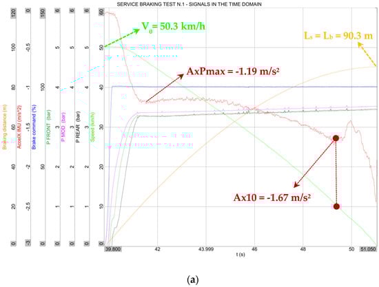
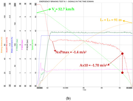
Figure 5.
Plots collecting the time histories of all main signals: (a) service braking, test n.1 of Section 4.1; (b) emergency braking, test n.1 of Section 4.3.
The following signals were measured and monitored:
- “Braking distance” [m] (the orange curve) is obtained as an integration of the speed.
- “AccelX IMU” [m/s2] (red curve) is the longitudinal deceleration measured by the IMU at a 100 Hz sample rate.
- “Brake command” [%] (blue curve) is the normalized position of the braking lever device actuated by the driver. The 100% value is obtained at the maximum admittable rotation of the lever in the service braking operation, while the driver has to rotate the lever to a further angle to initiate emergency braking operation, raising the brake command to 120% in this case.
- “P FRONT” [bar] (darker green curve) is the pressure in the cylinder of the front bogie.
- “P MOD” [bar] (magenta curve) is the modulated brake pressure which depends on the lever command position. Within 100% (service braking), its value raises to the maximum pressure, which sets the pressure of front and rear bogie’s brake cylinders; at 120% (emergency braking) the pressure cannot be modulated more by the driver, being in an emergency status, and the maximum pressure is delivered to both bogies (“P FRONT” and “P REAR” should be almost superimposed in an emergency braking like shown in the plot of Figure 5b).
- “P REAR” [bar] (cyan curve) is the pressure in the cylinder of the rear bogie.
- “Speed” [km/h] (green curve) is the measure of speed obtained by the xPro Nano device, eventually correcting the GPS signal with the information from IMU at 100 Hz to obtain an absolute error < 0.1 km/h.
The parameters obtained from the time histories are the initial speed of the train (V0) at instant when the braking command raises; the deceleration obtained when the maximum pressure is delivered to the bogies (AxPmax); the deceleration when speed drops to 10 km/h (Ax10); and the braking or stopping distance when the speed drops to zero and the train stops (Ls = Lb). Because the initial condition has been determined at the exact instant at which the brake command raises, the reaction distance Lr of Equation (1) is null in this case and Ls is coincident to Lb.
Zooming in on the first part of the plot of Figure 5a, a list of time delays can be measured (Figure 6) by comparing the synchronized channels, as it is the initial reference time set at the start of the brake command:
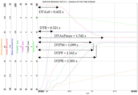
Figure 6.
Measured time delays in the first phase of the service braking (39.8 s to 42 s of Figure 5a), test n.1 of Section 4.1.
- DTB [s] is the time to reach the maximum braking command;
- DTAx0 [s] is the time to have a rate change in the deceleration;
- DTPM [s] is the time to reach 95% of the maximum modulated pressure (this parameter is calculated in service braking only);
- DTPF [s] and DTPR [s] are the times to reach 95% of the maximum pressure at the front or rear bogie;
- DTAxPmax [s] is the time to reach deceleration at maximum pressure.
Before proceeding with the analysis of results, one plot from a coasting test is shown in Figure 7. The test is performed to estimate the train deceleration due to aerodynamic drag and rolling resistance; it was performed on a flat part of the track with a travelled distance of about 110 m. The mean deceleration is estimated from the speed reduction.
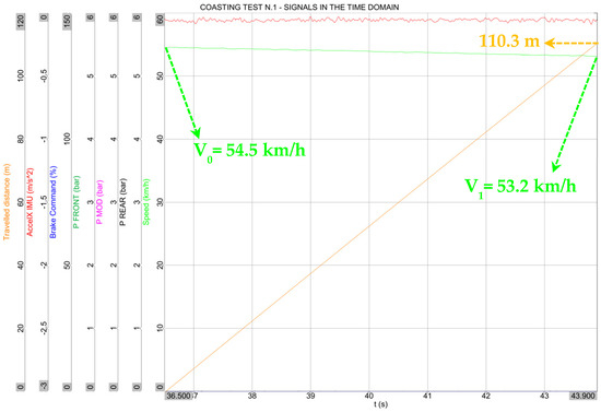
Figure 7.
Measured signals from of coasting test n.1 of Section 4.4.
4. Discussion of Results and Model Validation
4.1. Service Braking from 50 km/h
Table 4 collects the main quantities obtained in the four tests of service braking, showing good repeatability and a limited standard deviation. Unfortunately, the differences in initial speed, due to the limitations of speed control in this old train, led to a bigger deviation in the stopping distance value.
Table 4.
Quantities measured in service braking initiated at about 50 km/h.
4.2. Service Braking from 60 km/h
Additional service braking tests have been made at 60 km/h, which is the speed allowed in line maintenance operations with empty trains. The results from those tests where the initial speed is within 10% of exceeding the value have been reported in Table 5. Even in this case, the quantity with more relevant standard deviation is the stopping distance.
Table 5.
Quantities measured in service braking initiated at about 60 km/h.
4.3. Emergency Braking from 50 km/h
The results from four emergency braking tests from 50 km/h, which showed good repeatability and limited values of standard deviation, are summarized in Table 6.
Table 6.
Quantities measured in emergency braking initiated at about 50 km/h.
4.4. Coasting
The coasting tests led to identifying a mean value of deceleration (AxCoast) equal to −0.054 m/s2, with a low standard deviation, as reported in Table 7.
Table 7.
Quantities measured in coasting tests initiated at about 50 km/h.
4.5. Synthesis of Results of Braking Tests
The mean values and standard deviations of quantities obtained in the different braking tests are summarized in Table 8 and Table 9.
Table 8.
Mean values of quantities measured in service and emergency braking tests.
Table 9.
Standard deviation of quantities measured in service and emergency braking tests.
4.6. Validation of the Dynamics Model for Service Braking and Comparison to Empirical Formulas
The first validation step of the dynamics model consisted of the identification of the resistance coefficients A, B, and C from Equation (14), thus leading to the following values:
A = 1095 [N], B = 1.8 [Ns/m], C = 2.44 [Ns2/m2]
These values led to a perfect match of speed in tests n.1 and n.2, with a slight lower accuracy in test n.3, as shown in the plot of Figure 8 where the calculated speed signal is perfectly superimposed to the measured one in tests n.1 and n.2.
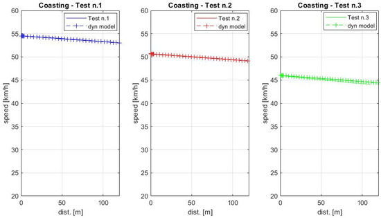
Figure 8.
Coasting tests: measured speed compared to speed computed by the dynamics model.
The second step was the identification of parameters for service braking. Plots of Figure 9 have been obtained using the rational model n.2 with the identified parameters shown in Table 10. In the same plots the stopping distance calculated using the Italian C.M. Formula (9) is marked by a circle.
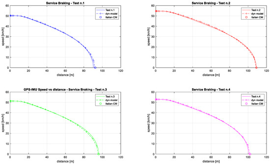
Figure 9.
Service braking from 50 km/h: validation of the dynamics model.
Table 10.
Service braking from 50 km/h: identified parameters for the different calculation methods.
Table 11 reports the estimated stopping distances using the presented methods, and the difference with respect to the measured values in the four service braking tests.
Table 11.
Service braking from 50 km/h: comparison of measured stopping distances and calculated ones with different methods.
Observing the negligible differences obtained with all models, one may suppose that the use of one of the empirical formulas for this local railway application could be the easier solution, but some doubts arise when observing the braking percentage values that have been identified to obtain the matching. These values are reported in Table 11, together with the other identified parameters.
As expected, the λ% value obtained from the dynamics model is the lowest because it tends to estimate the exact amount of total braking force required to simulate the service braking test. The value obtained from Italian C.M. is still acceptable for this train type, while all other values are not reasonable. It means that the application of Formulas (3), (4), and (6) to this local railway would have given poor results without performing any experimental test to estimate the parameters and instead using the suggested parameters that can be found in the literature references (Table 1). This is an important piece of advice that discourages the use of these formulas outside the boundaries of their generation rules. On the other hand, the development of the dynamics model, however, requires testing activities for model tuning, and a larger number of parameters have to be identified. Of course, the dynamics model gives the opportunity to retrieve more outputs besides the stopping distance, as shown in the plots of Figure 10, which present the comparison of different simulated signals with the corresponding measured ones.
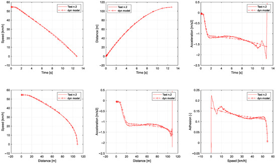
Figure 10.
Service braking from 50 km/h: outputs from the dynamics model for test n.3, and comparison with measured values.
When simulating the service braking starting from about 60 km/h, and using the same parameters of Table 11, test n.1 (Figure 11 and Table 12) is still well represented, while the dynamics model underestimates the stopping distance measured in tests 2 and 3 by about 20 m. These two experimental tests are reasonably less representative, because in test n.2 the train speed increases at the beginning and in test n.3 something unusual happened in the middle of the braking phase, as indicated by the black arrows in the plots of Figure 11 pointing to these highlighted occurrences.
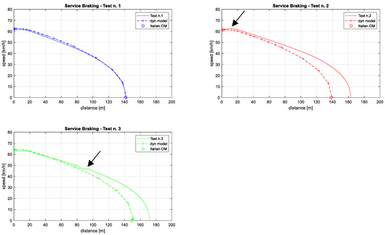
Figure 11.
Service braking from 60 km/h: validation of the dynamics model.
Table 12.
Service braking from 60 km/h: comparison of measured stopping distances and calculated ones with different methods.
4.7. Validation of the Dynamics Model for Emergency Braking and Comparison to Empirical Formulas
This step required the adjustment of some of the previously identified parameters, whose changed values are reported in bold in Table 13. The major effect is the expected increase in braking percentage, but the values to be introduced in (3), (4), and (6) still appear too high compared to values from the literature (Table 1). Amongst the empirical formulas, the Italian C.M. is considered the most consistent in terms of estimated braking percentage. The plots in Figure 12 and the differences in Table 14 show the validated dynamics model having the best fit of experimental data obtained for test n.1, while an underestimation of distance, within 10%, occurs for the other three tests.
Table 13.
Emergency braking from 50 km/h: identified parameters for the different calculation methods.
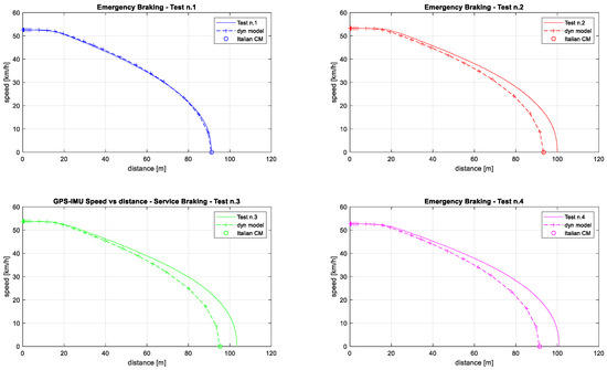
Figure 12.
Emergency braking from 50 km/h: validation of the dynamics model.
Table 14.
Emergency braking from 50 km/h: comparison of measured stopping distances and calculated ones with different methods.
Regarding the underestimation in tests 2 to 4, it likely depends on the increase in temperature in the brake shoes. This effect could be easily reproduced in the dynamics model by reducing the scaling factor in Equation (15). The plots of Figure 13 show the change in the outputs when the scaling factor is set at 0.9. The best fit is now obtained in tests n.2 to n.4, and the minimum error of braking distance (<0.4 m) is obtained in test n.3, whose additional plots are shown in Figure 14. This is a confirmation of the good accuracy of the dynamics model, which offers the possibility to quickly represent the influence of specific factors into the braking performance, such as the degradation of cast-iron shoes. It also paves the way for future analyses, such as those considering different functions of pad friction, substituting Equation (15) to account for braking pad upgrades with innovative materials, or introducing equations for thermal effects that require additional tests to be performed.
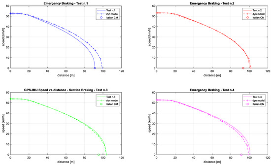
Figure 13.
Emergency braking from 50 km/h: validation of the dynamics model with a reduced friction coefficient of brake shoes.
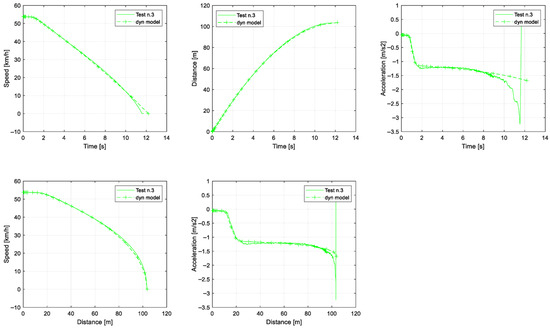
Figure 14.
Emergency braking from 50 km/h: dynamics model outputs of test n.3 with a reduced friction coefficient of brake shoes.
4.8. Use of the Dynamics Model for Exploring Different Scenarios in an Emergency Braking and Comparison to Empirical Formula at 50 km/h Initial Speed
As already mentioned, local railways like the one analyzed in this work cannot be compared to national ones because they have different safety systems and geometry characteristics. Additionally, accident data collection has been generally implemented only recently, thus reducing the applicability of standard risk management models. Recent changes in regulations pushed for the alignment of the safety and quality standards of local railways with the Italian national railway system. Braking efficiency and the correct estimation of stopping distance, especially in emergency situations at level crossings, are fundamental to the risk assessment process, and the use of an accurate but easily applicable calculation method for the braking phase has become a fundamental tool that has motivated railway management to push for this research.
Besides the very good results obtained in terms of the reproduction of experimental braking in dry track conditions—the only one that was possible to test at the current research stage—the calculation method can be used to quickly analyze different scenarios in terms of changes in the braking system performance and environmental conditions.
In Table 15, the stopping distance is calculated in the baseline configuration and with four modifications—track inclination, kp coefficient, scaling factor—from an exact initial speed of 50 km/h using both the dynamics model and the C.M. empirical formula. The results from the two methods are comparable (within a ±3% difference), but there is a fundamental distinction for the final cases. When trying to consider a reduction in the train’s braking efficiency, the dynamics model lets one make the calculation dependent on a physical parameter (kp or ), while the empirical formula requires the definition of a specific value of u scale factor (1.2 or 1.6 in the two considered cases) which has no physical meaning and cannot be hypothesized a priori, thus confirming the greater general applicability of the developed dynamics model. Moreover, an increase in pressure raising time tE in the definition of Y(t) function (Equation (16)) can be accounted for only by the dynamics model.
Table 15.
Emergency braking from exact 50 km/h: different calculation scenarios.
Additional calculations have been performed to estimate the effects of the friction model (Table 2) and track conditions on stopping distances. Besides the friction model n.2, which has already been used as a baseline, the n.1 and n.5 of Table 2 have been included in these additional calculations. Four levels of the maximum adhesion coefficient at null speed have been considered. They correspond to almost dry, perfectly clean (μ0 = 0.3), wet (μ0 = 0.2), moist and dirty (μ0 = 0.15), and highly contaminated (μ0 = 0.1).
The results reported in Table 16 clearly show that there is no change in stopping distance if μ0 is greater than 0.2. For this kind of aged train, this result is consistent with the characteristics of a brake system where the performance has been designed in the past to satisfy regulations that used lower values of μ0 even in dry track condition. The increase in stopping distance is relevant when μ0 drops below 0.15. This condition might occur in some portions of this local railway that are exposed to contamination by leaves in autumn, and the presence of ice or snow in winter. Finally, the use of the C.M. empirical formula requires, even for this evaluation, the assumption of consistent values of the u scale parameter.
Table 16.
Emergency braking from exact 50 km/h: results from different friction models and track conditions.
5. Conclusions
The results illustrated in the previous section have clarified two important aspects regarding the application of different braking calculation methods to a local railway with peculiar characteristics and old trains running.
Regarding the application of empirical formulas, the possibility to reach a satisfactory level of validation with respect to measured stopping distances imposed the use of unfeasible braking percentage values in Maison, Pedeluck, and Minden formulas. This fact determines the suggestion to skip these formulas for this specific railway system and running speeds, limiting the use of empirical formulas to the Italian C.M. one, where the identified values of braking percentage, even if higher than the dynamics model, are consistent.
The use of the proposed dynamics model can be regarded as a particularly good compromise in terms of the number of parameters to be identified and the obtained accuracy level. It perfectly fits the test outputs, while giving the possibility to separately evaluate the contributions of aspects to the train braking performance, such as the time delay in pressure delivery, the reduction in friction coefficient at brake shoes, the rational model of wheel–rail friction, and the maximum adhesion value depending on the track conditions.
From the point of view of local railway management, both reliable calculation approaches are considered an important add-on. The Italian C.M. formula with the experimentally identified parameters can be used in some contexts where it is crucial to have an easy to explain and consolidated formula with a few parameters. On the other hand, the more complicate dynamics model with this certified level of gained accuracy is an essential tool in the risk assessment process, providing the opportunity to evaluate several scenarios by using scaling coefficients related to physical quantities, as illustrated in Section 4.8, or being applied to different trains. The level of fidelity reached with this first version of the model motivates the investment towards future studies and experimental tests under different track conditions, braking system characteristics, or train type.
Author Contributions
Conceptualization, methodology, validation, formal analysis, investigation, data curation, and writing—original draft preparation, G.F.; writing—review and editing, G.F. and A.D.G.; project administration and supervision, A.D.G. All authors have read and agreed to the published version of the manuscript.
Funding
This research received no external funding; it was partially supported by the University of Catania within the internal academic project SICURI (PIACERI 24-26).
Data Availability Statement
The datasets presented in this article are not readily available because the data are part of an ongoing study.
Acknowledgments
The authors want to thank “Ferrovia Circumetnea” which made available the railway site and provided field assistance during the surveys, as well as DEWEsoft which allowed us to use the DAQs as a result of their support to universities.
Conflicts of Interest
The authors declare no conflicts of interest.
References
- European Union Agency for Railways. Report on Railway Safety and Interoperability in the EU 2024; European Union Agency for Railways: Valenciennes, France, 2024. [Google Scholar] [CrossRef]
- European Union Agency for Railways. Report on Railway Safety and Interoperability in the EU 2022; European Union Agency for Railways: Valenciennes, France, 2022. [Google Scholar] [CrossRef]
- Blumenfeld, M.; Lin, C.-Y.; Jack, A.; Abdurrahman, U.T.; Gerstein, T.; Barkan, C.P.L. Towards measuring national railways’ safety through a benchmarking framework of transparency and published data. Saf. Sci. 2023, 164, 106188. [Google Scholar] [CrossRef]
- Barney, D.; Haley, D.; Nikandros, G. Calculating train braking distance. In Conferences in Research and Practice in Information Technology; Australian Computer Society Inc.: Sydney, Australia, 2001; Available online: http://dl.acm.org/doi/pdf/10.5555/563780.563784 (accessed on 5 June 2025).
- Subotić, T.; Vasiljević, M. Influence of Train Stopping Distance and Overlap on the Railway Traffic Safety. In Proceedings of the 3rd International Scientific Conference “Transport for Today’s Society”, Bitola, North Macedonia, 14–16 October 2021. [Google Scholar] [CrossRef]
- Di Graziano, A.; Marchetta, V. A risk-based decision support system in local railways management. J. Rail Transp. Plan. Manag. 2021, 20, 100284. [Google Scholar] [CrossRef]
- Marchetta, V.; Di Graziano, A.; Contino, F. A methodology for introducing the impact of risk analysis in local railways improvements decisions. Transp. Res. Procedia 2023, 69, 424–431. [Google Scholar] [CrossRef]
- Profillidis, V.A. Train Dynamics. In Railway Management and Engineering, 4th ed.; Ashgate Publishing Limited: Farnham, UK, 2014; Section 18.11.2, Braking distance. [Google Scholar]
- Hoel, L.A.; Garber, N.J.; Sadek, A.W. Human, Vehicle, and Travelway Characteristics. In Transportation Infrastructure Engineering: A Multimodal Integration, SI Edition; Cengage Learning: Stamford, CT, USA, 2011; pp. 111–117. [Google Scholar]
- Magelli, M. Development of Numerical and Experimental Tools for the Simulation of Train Braking Operations. Ph.D. Thesis, Politecnico of Turin Italy, Torino, Italy, 2023. Available online: https://iris.polito.it/handle/11583/2978155 (accessed on 5 June 2025).
- Bosso, N.; Magelli, M.; Zampieri, N. Development and validation of a new code for longitudinal train dynamics simulation. Proc. Inst. Mech. Eng. Part F J. Rail Rapid Transit 2021, 235, 286–299. [Google Scholar] [CrossRef]
- Wu, Q.; Cole, C.; Spiryagin, M. Train braking simulation with wheel-rail adhesion model. Veh. Syst. Dyn. 2020, 58, 1226–1241. [Google Scholar] [CrossRef]
- Günay, M.; Korkmaz, M.E.; Özmen, R. An investigation on braking systems used in railway vehicles. Eng. Sci. Technol. Int. J. 2020, 23, 421–431. [Google Scholar] [CrossRef]
- Kustosz, J.; Goliwas, D.; Kaluba, M. A tool for calculating braking distances of rail vehicles. Pojazdy Szyn. 2022, 3–4, 15–19. [Google Scholar] [CrossRef]
- Liu, K.; Wang, Z.; Zhang, M.; Luo, Y.; Wang, Y.; Shen, Y.; Zhang, W. Influence of leakage during cyclic pneumatic braking on the dynamic behavior of heavy-haul trains. Mech. Syst. Signal Process. 2025, 228, 112490. [Google Scholar] [CrossRef]
- Chen, J.; Yu, C.; Cheng, Q.; Guan, Y.; Zhang, Q.; Li, W.; Ouyang, F.; Wang, Z. Research on friction performance and wear rate prediction of high-speed train brake pads. Wear 2023, 514, 204564. [Google Scholar] [CrossRef]
- Ehret, M.; Hohmann, E.; Heckmann, A. On the modelling of the friction characteristics of railway vehicle brakes. Int. J. Rail Transp. 2022, 11, 50–68. [Google Scholar] [CrossRef]
- De Falco, G.; Russo, G.; Ferrara, S.; De Soccio, V.; D’Anna, A. Sustainable design of low-emission brake pads for railway vehicles: An experimental characterization. Atmos. Environ. X 2023, 18, 100215. [Google Scholar] [CrossRef]
- Meacci, M.; Shi, Z.; Butini, E.; Marini, L.; Meli, E.; Rindi, A. A railway local degraded adhesion model including variable friction, energy dissipation and adhesion recovery. Veh. Syst. Dyn. 2020, 59, 1697–1718. [Google Scholar] [CrossRef]
- Kalker, J.J. A Fast Algorithm for the Simplified Theory of Rolling Contact. Veh. Syst. Dyn. 1982, 11, 1–13. [Google Scholar] [CrossRef]
- Vollebregt, E.; Schuttelaars, H. Quasi-static analysis of two-dimensional rolling contact with slip-velocity dependent friction. J. Sound Vib. 2012, 331, 2141–2155. [Google Scholar] [CrossRef]
- Zewang, Y.; Mengling, W.; Chun, T.; Jiajun, Z.; Chao, C. A Review on the Application of Friction Models in Wheel-Rail Adhesion Calculation. Urban Rail Transit 2021, 7, 1–11. [Google Scholar] [CrossRef]
- Polach, O. Creep forces in simulations of traction vehicles running on adhesion limit. Wear 2005, 258, 992–1000. [Google Scholar] [CrossRef]
- Vollebregt, E.; Six, K.; Polach, O. Challenges and progress in the understanding and modelling of the wheel–rail creep forces. Veh. Syst. Dyn. 2021, 59, 1026–1068. [Google Scholar] [CrossRef]
- Chen, H.; Ban, T.; Ishida, M.; Nahahara, T. Experimental investigation of influential factors on adhesion between wheel and rail under wet conditions. Wear 2008, 265, 1504–1511. [Google Scholar] [CrossRef]
- Zhou, J.; Zhu, W.; Tian, C.; Wu, M.; Zhai, G. Experimental investigation of wheel rail adhesion under leaf contamination conditions. Int. J. Rail Transp. 2024, 1–20. [Google Scholar] [CrossRef]
- Chang, C.; Chen, B.; Cai, Y.; Wang, J. Experimental investigation of high-speed wheel-rail adhesion characteristics under large creepage and water conditions. Wear 2024, 540, 205254. [Google Scholar] [CrossRef]
- Rochard, B.P.; Schmid, F. A review of methods to measure and calculate train resistances. Proc. Inst. Mech. Eng. Part F J. Rail Rapid Transit 2020, 214, 185–199. [Google Scholar] [CrossRef]
- Sawczuk, W.; Kołodziejski, S.; Rilo Cañás, A.M. Determination of the resistance to motion of a cargo train when driving without a drive. Combust. Engines 2024, 197, 64–70. [Google Scholar] [CrossRef]
- Szanto, F. Rolling resistance revisited. In Proceedings of the Conference on Railway Excellence—CORE 2016, Melbourne, Australia, 16–18 May 2016. [Google Scholar]
- Bochet, H. Du Frottement de Glissement Spécialement sur les Rails des Chemins de Fer: Sa Variation Avec la Vitesse, Formule Représentative; Dalmont et Dunod: Paris, France, 1858. [Google Scholar]
- Cantone, L. TrainDy: The New Union Internationale Des Chemins de Fer Software for Freight Train Interoperability. Proc. Inst. Mech. Eng. Part F J. Rail Rapid Transit 2010, 225, 57–70. [Google Scholar] [CrossRef]
- Zhang, W.; Chen, J.; Wu, X.; Jin, X. Wheel/rail adhesion and analysis by using full scale roller rig. Wear 2002, 253, 82–88. [Google Scholar] [CrossRef]
- Sirong, J.M. Traction Calculation. In Principles of Railway Location and Design; Sirong, Y., Ed.; Academic Press: Cambridge, MA, USA, 2018; pp. 73–157. [Google Scholar] [CrossRef]
- Spiroiu, M.A. About the influence of wheel-rail adhesion on the maximum speed of trains. MATEC Web Conf. 2018, 178, 06004. [Google Scholar] [CrossRef][Green Version]
- Lozano, J.A.; Félez, J.; de Dios Sanz, J.; Mera, J.M. Railway Traction. In Reliability and Safety in Railway; Perpiñá, X., Ed.; InTech: London, UK, 2012. [Google Scholar]


Disclaimer/Publisher’s Note: The statements, opinions and data contained in all publications are solely those of the individual author(s) and contributor(s) and not of MDPI and/or the editor(s). MDPI and/or the editor(s) disclaim responsibility for any injury to people or property resulting from any ideas, methods, instructions or products referred to in the content. |
© 2025 by the authors. Licensee MDPI, Basel, Switzerland. This article is an open access article distributed under the terms and conditions of the Creative Commons Attribution (CC BY) license (https://creativecommons.org/licenses/by/4.0/).