Modal Analyses of Flow and Aerodynamic Characteristics of an Idealized Ground Vehicle Using Dynamic Mode Decomposition

Abstract

This study investigates the connection between coherent structures in the flow around a vehicle and the aerodynamic forces acting on its body. Dynamic Mode Decomposition (DMD) was applied to analyze the flow field of a squareback Ahmed body at $R{e}_H=7.7\times {10}^5$. DMD enabled the identification of coherent structures in the near and far wake by isolating their individual oscillation frequencies and spatial energy distributions. These structures were classified into three regimes based on their underlying mechanisms: symmetry breaking, bubble pumping, and large-scale vortex shedding in range of $St\le 0.2$. The energy contributions of these flow regimes were quantified across different regions of the flow field and compared to the aerodynamic forces on the body. Additionally, the linear correlation between pressure and velocity components was examined using Pearson correlation coefficients of DMD spectral amplitudes. The locations of maximum and minimum correlation values, as well as their relationship to energy contributions, were identified and analyzed in detail.

1. Introduction

The aerodynamic performance of a ground vehicle is predominantly influenced by the flow structures surrounding its body, particularly by the wake region where flow separation occurs. In general, for blunt, bluff-bodied vehicles, this separation leads to the formation of complex shear layers and vortices, which interact to create a large, low-pressure recirculation region behind the vehicle, and plays a dominant role in contributing to the overall vehicle drag. The flow structures, whether generated at the edges of the vehicle or within the wake, have a significant impact on the aerodynamic forces acting on the vehicle, particularly drag. Gaining a detailed understanding of these flow contributions is crucial for optimizing vehicle designs to minimize drag, improve vehicle stability and controllability for autonomous vehicles, and enhance overall performance.

Flows over real-world ground vehicles are highly complex, and their CAD models and experimental data are often proprietary to specific Original Equipment Manufacturers, or OEMs. To overcome this limitation, researchers use idealized vehicle models to study fundamental flow characteristics. Several such geometries exist in the literature, such as the SAE Body [1] and Windsor Body [2]. However, the Ahmed Body [3] still remains the most widely used model among researchers, which features a basic geometric shape with a variable slant at the rear, allowing researchers to analyze flow separation, wake structures, and drag characteristics. In this study, we focus on the squareback (0° slant) variant of the Ahmed body. This simplified form is widely used in the literature for investigating bi-stability and bluff-body wake dynamics, and is commonly referred to as the squareback or zero-slant Ahmed body. The slant angle can be varied to represent a wide range of vehicle shapes, such as sedans, station-wagon, and SUVs. Due to its simple yet well-defined shape and the availability of extensive experimental and numerical data, the Ahmed Body has become the most widely used benchmark for validating computational fluid dynamics (CFD) simulations and understanding the aerodynamic behavior of road vehicles.

One of the significant features of the Ahmed Body’s wake dynamics, as well as that of other ground vehicles, is the so-called bi-stability (see Grandemange et al. [4]), which has a major impact on the vehicle’s aerodynamic performance. The bi-stability phenomenon implies the existence of two alternating preferred asymmetric states in the vehicle wake. This alternation results in a statistically symmetric wake when averaged over a long time. The transitions between these two states follow the characteristics of a stationary Markov process, meaning the wake switches unpredictably but with consistent statistical properties. These transitions generate unsteady side forces on the vehicle, affecting its lateral stability and contributing to aerodynamic drag by altering the vehicle’s base pressure. Volpe et al. [5] observed that the time scale of this bi-stability is large, approximately 800 $U_{\infty }/H$, where $U_{\infty }$ and H are the freestream velocity and height of the vehicle, respectively. As such, it requires a long data sampling time to properly characterize stable positions for both positive ($\mathcal{P}$) and negative ($\mathcal{N}$) states. Existing literature shows that several factors influence the behavior of bi-stability, such as the yaw angle [5] and ground clearance [6]. Additionally, Kang et al. [7] showed that a thick boundary layer on the ground can suppress bi-modality in the wake of an Ahmed body, implying the importance of proper ground emulations for experimental studies.

Another key feature observed in the wake dynamics bi-modality is known as the bubble pumping. This is characterized by periodic inflation and deflation of the wake recirculation zone, which affect the vehicle’s stability and aerodynamic forces. Khalighi [8] identified this low-frequency phenomenon, which corresponds to a Strouhal number of 0.07 ($St=f\times L/U_{\infty }$ where f and L are the frequency in Hz and characteristic length, respectively). They described it as the periodic interaction between the upper and lower parts of the trapped vortex in the near wake, which moves the stagnation point along the stream direction. Volpe et al. [5] further investigated bubble pumping, identifying its strong presence in the recirculation bubble’s shear layers, and Podvin et al. [9] calculated its energy contribution to be about 1% of the total kinetic energy.

Other important dynamic structures observed in the flow around bluff bodies are vortex shedding from the lateral and upper/lower edges of the rear fascia. These periodic vortices result from flow separation at sharp edges, generating coherent structures that play a significant role in the wake’s evolution and vehicle drag. Grandemange et al. [4] identified two significant modes, with Strouhal numbers of 0.127 and 0.174, attributed to vortex shedding from the lateral and top/bottom edges, respectively, with the lateral mode being more energetic. Several studies have reported vortex-shedding structures across a range of Strouhal numbers, with the specific values depending on factors such as Reynolds number, ground clearance, and body aspect ratio, etc.

In general, three important frequency ranges emerged from our survey of vortex-shedding characteristics observed in flows past simplified ground vehicles, as listed below. Note that it is difficult to assign a global Strouhal number to these vortex-shedding structures, as their values depend on factors such as Reynolds number, ground clearance, and body aspect ratio. Variations in these parameters across the studies explain the discrepancies in the reported Strouhal numbers:

• The Strouhal range of $0.12\le St\le 0.14$ is associated with vortex shedding from the lateral wall near the wake (cf. [4,5,6,7,10]).
• Vortex shedding from the bottom and top edges occurs within the range of $0.15\le St\le 0.19$ ( cf. [4,5,6,7,9,10,11,12,13]).
• Researchers have also observed another significant coherent structure emerging from the lateral walls, mostly pairing in the far wake regions within the range of $0.19<St\le 0.24$ (cf. [9,11,14]).

As mentioned earlier, controlling these dynamic wake structures, such as vortex shedding and bi-stability, is crucial for reducing drag and optimizing the aerodynamic performance of vehicles. Various control techniques, including active and passive methods, have been developed to manipulate these wake structures. Evrard et al. [15] achieved a 9% drag reduction using a cavity, while Krajnovic et al. [16] utilized vortex generator cylinders to delay separation. Grandemange et al. [17] employed control cylinders to mitigate bi-stability, reducing pressure drag by 4–9%. More recently, active control techniques have gained popularity due to their flexibility and effectiveness. Open-loop forcing with jets, either constant or pulsed, can reduce drag by up to 10% [11,18]. Closed-loop feedback control, such as that used by Li et al. [19] with lateral slit jets and pressure sensors, has been shown to mitigate bimodal wake dynamics through unsteady shear layer forcing. Bruneau et al. [20] combined closed-loop control with passive techniques, achieving a drag reduction of nearly 30%.

To design an efficient and effective flow-control system, it is essential to ensure that the application of external forcing yields maximum aerodynamic benefit with minimal energy input. This requires not only a fundamental understanding of the underlying flow structures but also a precise knowledge of where, when, and how such interventions should be applied. Therefore, identifying the spatial and temporal energy distribution of flow features becomes critical for optimizing control strategies in a cost-effective manner. Although many studies have investigated vehicle wake dynamics, few have shown where coherent structures gain the most energy or how their energy is distributed across the flow field. It can improve our understanding of the interactions between flow structures, energy distribution, and aerodynamic performance, helping to develop more effective drag reduction techniques.

We investigated the flow dynamics around the idealized Ahmed body [3] at a high Reynolds number of $Re=7.7\times {10}^5$, using the Ahmed body height and freestream velocity as the characteristic length and velocity scales, respectively. Proper Orthogonal Decomposition (POD) [21] is first used for modal extraction validation, followed by Dynamic Mode Decomposition (DMD) [22] to extract dominant flow structures and quantify their energy distribution. Unlike traditional modal methods such as POD, DMD provides the unique ability to decompose the flow field into spatial modes while assigning a distinct frequency to each, enabling the analysis of how energetic structures evolve across both space and time. Although DMD has been applied in a few studies related to road vehicle aerodynamics [23,24,25,26,27], these applications are typically restricted in both temporal and spatial resolution. In contrast, the present study leverages the high spatial fidelity of IDDES by collecting data over multiple finely resolved two-dimensional planes, rather than relying on coarse three-dimensional fields, when fine-resolution 3D would be computationally infeasible with available resources at this Reynolds number. The results identify distinct frequency regimes associated with symmetry breaking, bubble pumping, and vortex shedding, highlighting the need for targeted control strategies.

In the following sections, we will analyze the time history of the drag force, mean flow topology, POD decomposition, and its frequency spectrum, comparing our results with the existing literature. This will be followed by an in-depth investigation of DMD mode shapes and their temporal dynamics. Additionally, we will examine the energy distribution of dynamic structures in both spatial and temporal domains. Lastly, we will study the correlation between field variables at different locations using the DMD frequency spectrum.

2. Simulation Methodology

2.1. Governing Equations and Turbulence Modeling

In this study, the flow past a squareback or zero-degree slant angle Ahmed body, which resembles the rear end of an SUV, was simulated using the commercial CFD code STAR-CCM+, version 20.2. This code employs the finite volume method (FVM) on an unstructured grid to resolve the flow field. The simulations solve the incompressible 3D Navier–Stokes equations, which consist of the momentum and continuity equations represented by Equations (1) and (2), respectively, using Einstein notation, in which repeated indices, such as i or j, indicate summation over all possible values.

$$\begin{array}{ccc}\hfill {\displaystyle \frac{\partial \rho }{\partial t}}+{\displaystyle \frac{\partial \left(\rho u_i\right)}{\partial x_i}}& =& 0\hfill \end{array}$$

(1)

$$\begin{array}{ccc}\hfill {\displaystyle \frac{\partial \left(\rho u_i\right)}{\partial t}}+{\displaystyle \frac{\partial \left(\rho u_i{u}_j\right)}{\partial x_j}}& =& -{\displaystyle \frac{\partial p}{\partial x_i}}+{\displaystyle \frac{\partial {\tau }_{ij}}{\partial x_j}}+\rho f_i\hfill \end{array}$$

(2)

In the above equations, $\rho$ is the fluid density, $u_i$ and $u_j$ denote the velocity components in the i-th and j-th directions, respectively, t represents time, and $x_i$ is the spatial coordinate in the i-th direction. The term ${\tau }_{ij}\equiv 2\mu s_{ij}$ is the viscous stress tensor, and $f_i$ represents the external body force per unit volume acting in the i-th direction, such as gravitational or electromagnetic forces, which are negligible in vehicle aerodynamics. With $\mu$ as the fluid dynamic viscosity, the strain rate tensor $s_{ij}$ is defined as

$$s_{ij}={\displaystyle \frac{1}{2}}\left({\displaystyle \frac{\partial u_i}{\partial x_j}}+{\displaystyle \frac{\partial u_j}{\partial x_i}}\right)$$

(3)

While the Navier–Stokes equations describe the full dynamics of fluid flow, solving them directly requires resolving all scales of motion, from large eddies to the smallest viscous dissipative scales. Direct Numerical Simulation (DNS) is the most accurate approach to solve the Navier–Stokes equations by fully resolving these scales, but it is computationally expensive and often impractical for high Reynolds number flows, such as those around ground vehicles. To address this challenge, turbulence modeling approaches are employed to approximate the effects of unresolved scales, providing a computationally efficient alternative while capturing the essential features of turbulent flows.

As such, for practical reasons, this study uses a Shear Stress Transport (SST) [28] based variant of the Improved Delayed Detached-Eddy Simulation (IDDES) [29] model to resolve the transient turbulent flow field. IDDES is a hybrid turbulence model that combines the advantages of Reynolds-Averaged Navier–Stokes (RANS) and Large Eddy Simulation (LES) approaches. In the IDDES approach employed in this study, the SST $k-\omega$ model is used for resolving near-wall turbulence transience.

The development of IDDES was motivated by the need for a model that can accurately capture both near-wall turbulence (using RANS) and large-scale unsteady structures (using LES) in complex flows, such as those around bluff bodies, while maintaining computational affordability. The IDDES approach, balancing accuracy and cost-effectiveness, has recently gained significant popularity for ground vehicle external aerodynamics applications. IDDES evolves from the Detached Eddy Simulation (DES) approach originally proposed by Spalart and his coworkers [30]. In the DES approach, there is a switch between the RANS model near the wall and the outer layer with local grid refinement, which can lead to inaccurate log-law capturing. Furthermore, erroneous activation of the DES limiter in the RANS region can potentially cause artificial flow separation due to grid resolution. To mitigate this problem, Shur et al. [31] proposed providing shielding against grid-induced separation. IDDES improves upon DDES by providing better grid-induced separation shielding, enabling wall-modeled LES, and addressing log-layer mismatch for more accurate and flexible simulations of high Reynolds number flows.

DMD, as originally introduced by Schmid [22], was demonstrated using data from particle image velocimetry (PIV) and direct numerical simulation (DNS), both capable of capturing a wide range of spatial and temporal flow scales without the need for turbulence modeling. However, for high Reynolds number automotive flows, these methods are often computationally prohibitive. As an alternative, coarser CFD data obtained using turbulence models are commonly employed. Muld et al. [32] evaluated the suitability of DES for input into POD and DMD and confirmed its viability for extracting coherent structures. Bounds et al. [33] further supported the effectiveness of IDDES in simulating complex vehicle flow scenarios, including two-vehicle platooning and single-body wakes. Additional assessments of IDDES performance, specifically for Ahmed body simulations, are available in the works of Ashton et al. [34] and Guilmineau et al. [35]. Broader comparisons of IDDES and RANS methods in capturing turbulent structures are presented in studies such as Fu et al. [36] and Misar et al. [37]. Validation of the CFD dataset used in the present work—benchmarked against the experimental results of Volpe et al. [5]—was previously documented in our own publication [38], to which the reader is referred for further technical details.

2.2. Numerical Setup

The squareback Ahmed body was placed inside a computational domain measuring $30L\times 30W\times 30H$ in the streamwise, lateral, and vertical directions, respectively. The characteristic dimensions of the Ahmed body are the following: length $L=1044\mathrm{mm}$, width $W=389\mathrm{mm}$, and height $H=288\mathrm{mm}$. These dimensions yield a blockage ratio of only 0.1% relative to the frontal area, minimizing wall interference effects. The model was positioned $10L$ downstream from the inlet boundary. At the inlet, a uniform freestream velocity of 40 m/s was imposed, corresponding to a Reynolds number based on body height of $R{e}_H=7.7\times {10}^5$. This velocity was selected to ensure Reynolds number independence of the flow, as reported by Lahaye et al. [14]. Pressure outlet conditions were applied at the downstream boundary, and symmetry (zero-gradient) conditions were used for the top and side boundaries. A no-slip, moving-ground condition was applied at the floor, with a surface velocity equal to the freestream velocity to replicate realistic road conditions.

The computational domain was discretized using an unstructured hexahedral mesh generated with the trimmed-cell mesher in STAR-CCM+. A base cell size of $0.014H$ was used throughout the vehicle surface and underbody. The wake region was refined to a mesh size of $0.007H$, while in the far wake it was coarsened to $0.028H$. Figure 1 illustrates the mesh scheme. Near-wall treatment involved 28 prism layers with a total thickness of $0.035H$ and a first-layer height of $1.7\times {10}^{-6}H$, ensuring $y^{+}<1$ for more than 99% of the wall-adjacent cells (Figure 2). The non-dimensional wall distance is defined as $y^{+}=y{u}_{\tau }/\nu$, where $\nu$ is the kinematic viscosity and $u_{\tau }$ is the friction velocity.

An implicit, unsteady, segregated incompressible solver was used to simulate the flow. A second-order temporal discretization was employed with a non-dimensional time step of $\mathrm{\Delta }t=0.0138L/U_{\infty }$. The momentum and turbulence equations were discretized using a second-order upwind scheme. The Algebraic Multigrid (AMG) solver with a V-cycle strategy was applied to enhance convergence of the linearized equations. The simulation was run for a total physical time of $556L/U_{\infty }$, with the first $276L/U_{\infty }$ discarded to eliminate transients. The remaining time was used for ensemble averaging over a sliding window of equal length. This ensured convergence of statistical quantities and enabled resolution of low-frequency coherent structures, with the lowest resolved frequency being 0.5 Hz, corresponding to a Strouhal number of $St=3.6\times {10}^{-3}$.

3. Decomposition Algorithms

Two decomposition techniques are employed in this study: (a) POD [21], and (b) DMD [22]. These methods decompose the flow field into spatial and temporal modes. The flow variables include the instantaneous streamwise (u), spanwise (v), and vertical (w) velocity components, along with pressure (p). These scalar fields are analyzed on selected planes:

(a)

x-planes at $x/L=1.1$, $1.2$, $1.5$, 2, and $2.5$, where $x=0$ denotes the front nose,

(b)

y-planes at $y/W=0$, $0.25$, and $0.5$, with $y=0$ aligned along the body centerline,

(c)

z-planes at $z/H=0$, $0.25$, $0.5$, $0.75$, and 1, where $z=0$ aligns with the underbody.

The locations of these planes are illustrated in Figure 3. In addition, pressure data from the vehicle surface is also analyzed.

The spatial modes are used to identify coherent structures in various regions of the flow—on and around the vehicle body, within the wake, and farther downstream—while the temporal modes capture the time evolution of these structures. For both decomposition methods, snapshots of the flow field are organized into a vector form for each flow quantity, described by the following equation:

$$X_i=\left[x_i^1,x_i^2,x_i^3,\dots ,x_i^N\right]$$

(4)

Here, the subscript i refers to the i-th grid element in a domain with M total elements, and the superscript indicates the time index of the snapshot. Collecting these vectors across all grid points forms the following data matrix:

$$\mathbf{X}=\left[\begin{array}{ccc}{x}_1^1& \dots & x_1^N\\ ⋮& \ddots & ⋮\\ x_M^1& \dots & x_M^N\end{array}\right]$$

(5)

POD, originally introduced by Lumley [21], is a widely used technique in fluid dynamics for extracting dominant flow structures and reducing model complexity. In this method, the flow field is decomposed into a series of orthogonal spatial basis functions modulated by time-dependent coefficients. The method relies on constructing the covariance matrix $\mathbf{C}$ of the data matrix $\mathbf{X}$ as

$$\mathbf{C}={\displaystyle \frac{1}{N-1}}{\mathbf{X}}^T\mathbf{X}$$

(6)

The eigenvectors and eigenvalues of $\mathbf{C}$ are then computed and ordered from highest to lowest energy contribution:

$$\mathbf{C}\mathbf{\Phi }=\mathbf{\Phi }\mathbf{\Lambda }$$

(7)

Here, $\mathbf{\Phi }$ contains the eigenvectors (spatial modes), and $\mathbf{\Lambda }$ is a diagonal matrix of eigenvalues representing mode energies.

Sirovich [39] later introduced the snapshot POD method, which is more efficient for large-scale datasets. Alternatively, Singular Value Decomposition (SVD) offers a numerically stable implementation. In SVD, the matrix $\mathbf{X}$ is factorized as

$$\mathbf{X}=\mathbf{U}\mathbf{\Sigma }{\mathbf{V}}^T$$

(8)

where $\mathbf{U}$ and $\mathbf{V}$ are unitary matrices, and $\mathbf{\Sigma }$ contains the singular values representing mode energies. In this study, an economy (reduced) SVD is used.

DMD is another decomposition technique used here, which provides a linear dynamical model of the flow. Unlike POD, DMD associates each mode with a single frequency and decay/growth rate, making it well-suited for studying unsteady coherent structures. To apply DMD, the data matrix $\mathbf{X}$ is split into two matrices offset by one timestep:

$${\mathbf{X}}^{\left(k\right)}=\left[\begin{array}{ccc}{x}_1^1& \dots & x_1^{N-1}\\ ⋮& \ddots & ⋮\\ x_M^1& \dots & x_M^{N-1}\end{array}\right],{\mathbf{X}}^{(k+1)}=\left[\begin{array}{ccc}{x}_1^2& \dots & x_1^N\\ ⋮& \ddots & ⋮\\ x_M^2& \dots & x_M^N\end{array}\right]$$

(9)

The system is assumed to evolve linearly between time steps:

$${\mathbf{X}}^{(k+1)}\approx \mathbf{A}{\mathbf{X}}^{\left(k\right)}$$

(10)

where $\mathbf{A}$ is a linear operator that maps the flow field forward in time. Since ${\mathbf{X}}^{\left(k\right)}$ is typically not square, its pseudoinverse is computed via SVD, and the matrix $\mathbf{A}$ is given by

$$\mathbf{A}={\mathbf{X}}^{(k+1)}\mathbf{V}{\mathbf{\Sigma }}^{-1}{\mathbf{U}}^{*}$$

(11)

The eigenvalue $\mathbf{\Lambda }$ of matrix $\mathbf{A}$ can be represented in complex form as $\lambda =a+ib$, where a denotes the real component, associated with the mode’s growth or decay over time, and b represents the imaginary component, corresponding to the mode’s oscillation frequency:

$$\omega ={\displaystyle \frac{ln\left(\lambda \right)}{\mathrm{\Delta }t}}={\displaystyle \frac{ln(a+ib)}{\mathrm{\Delta }t}}$$

(12)

The reconstructed flow field at time t can be expressed as

$${\displaystyle \frac{d\mathbf{X}}{dt}}=\mathbf{A}\mathbf{x}\to x_{(i,t)}=\sum _{k=1}^n{\mathbf{\Phi }}_k{e}^{{\omega }_{k}t}{b}_k$$

(13)

Here, ${\mathbf{\Phi }}_k$ are the spatial DMD modes, and $b_k$ are the modal amplitudes determined by projecting the initial condition onto each mode.

In this study, snapshots were collected at a sampling frequency of 2 kHz for a total time window of 2 s. Additionally, mean-subtracted DMD was applied to isolate unsteady flow structures from the steady background. A comprehensive explanation of parameter selection, including sampling rate, time window, and convergence assessment, is available in our prior work [38].

4. Results and Discussion

This section analyzes the aerodynamic characteristics of the squareback Ahmed body by examining mean flow properties and dominant flow dynamics. Modal decomposition techniques of POD and DMD are used to extract key dynamic structures and assess their energy distribution, contribution, and correlation. The findings are compared with established literature to provide insights into the dynamic behavior of flow and potential control strategies.

4.1. Drag Force

In this section, we analyze the drag force on the Ahmed body, a critical aerodynamic characteristic for optimizing vehicle fuel consumption. We present the time histories of pressure drag, friction drag, and base drag forces separately and compare them to results reported in the existing literature, including numerical and experimental studies. This comparative analysis serves to validate our findings and highlight key similarities and differences in drag predictions across various methodologies and setups. In this study, side and lift forces are not considered. The side force is omitted due to the geometric symmetry of the Ahmed body and the absence of side wind effects, which result in negligible lateral force. Lift force is also excluded, as the squareback configuration primarily generates wake-induced pressure drag, and contribution of lift to the overall aerodynamic performance is expected to be relatively small.

The total drag force, $F_D$, acting on the body is the sum of the pressure and friction drag. Understanding the contributions of both pressure and friction drag is crucial for accurately assessing the aerodynamic performance of the vehicle body. To facilitate more accurate comparisons across different scales, shapes, and flow conditions, it is best to express the force as a non-dimensional quantity, the coefficient of drag ($C_D$). With A denoting the characteristic area, which in this study is the frontal area of the vehicle, this is expressed as

$$C_D={\displaystyle \frac{F_D}{0.5\rho A{U}_{\infty }^2}}$$

(14)

Analyses of the collected data show that the mean pressure drag coefficient is 0.261, with an RMS fluctuation of 0.009, representing 3.5% of the mean value. In contrast, the friction drag coefficient has a mean value of 0.041 and an RMS fluctuation of $1.02\times {10}^{-4}$, which accounts for approximately 0.3% of its mean value. The mean total drag coefficient, $C_D$, in this study is 0.302, with the pressure drag contributing 85% and the friction drag accounting for the remaining 15%.

The low-pressure region in the wake behind the squareback Ahmed body forms as the flow separates from the sharp edges of the body. This low-pressure region generates a substantial suction force that pulls the vehicle backward, significantly contributing to the total drag, commonly referred to as base drag. Understanding base drag provides valuable insights into the interaction between shear layers and wake dynamics. According to previous research, base drag in square bluff bodies can account for 50–70% of the total drag. For the current study, the base drag is 0.216, contributing 72% to the total drag, which aligns well with results reported in other studies. The calculated RMS fluctuation of base drag in the present study is 0.009, which represents 4% of the mean value of the base drag.

To verify the grid independence of the numerical solution, a series of simulations were conducted with progressively refined mesh sizes ranging from $0.083H$ to $0.014H$. As shown in

Table 1. Mesh independence study: variation of total drag coefficient $C_D$ with mesh size.

$\mathrm{\Delta }\mathit{x}/\mathit{H}$	Total Cells (M)	${\mathit{C}}_{\mathit{D}}$
0.083	0.5	0.340
0.035	3.0	0.315
0.021	9.0	0.301
0.014	27.0	0.302

, the drag coefficient stabilizes as the mesh is refined, with less than 0.5% variation observed between the $0.021H$ and $0.014H$ cases. This confirms that the $0.014H$ base mesh, combined with a wake-region refinement to $0.007H$, provides grid-independent results and sufficient spatial resolution to accurately capture the dominant aerodynamic features of the flow.

The computed total drag coefficient of 0.302 shows good agreement with the values reported in other experimental and numerical studies. The total drag coefficient for the squareback Ahmed body reported in the literature varies within the range of 0.250 to 0.364, corresponding to a variation of 114 counts. In the original experimental study by Ahmed et al. [3], the total drag coefficient is reported as 0.250. The Reynolds number in that work is $1.7\times {10}^6$, corresponding to a freestream velocity of $60\mathrm{m}/\mathrm{s}$, which is significantly higher than in many other studies. Another study conducted by Lahaye et al. [14] at a similar Reynolds number ($R{e}_H=1.93\times {10}^6$) reports a total drag coefficient of 0.364 for a 7/10-scaled squareback Ahmed body. This value is approximately 45% higher than the original study by Ahmed. Such discrepancies have also been observed in other experimental and numerical studies related to the squareback Ahmed body. Apart from the effect of the Reynolds number, discrepancies can arise due to differences in wind tunnel or numerical setups, such as blockage ratio, inlet turbulence intensity, and ground clearance. Additionally, there are Ahmed body models with varying aspect ratios of height, width, and length, and not all studies use the same aspect ratio as the original work. Even minor differences, such as the sharpness of edges or the shape of slants, can lead to significant variations in drag values. A summary of various experimental and numerical studies reporting different drag coefficients for the Ahmed body is provided in

Table 2. Summary of total and baseline drag values across various studies.

Author	Geometry	${\mathbf{Re}}_{\mathbf{H}}$	Method	${\mathbf{C}}_{\mathbf{D}}$	${\mathbf{C}}_{\mathbf{D},\mathbf{base}}$
Ahmed et. [3]	1:1 scale	$1.7\times {10}^6$	Exp	0.250	0.177
Brackston et al. [40]	1:1 scale	O(${10}^5$)	Exp	0.347	-
Dalla et al. [23]	≈ 3.2:1	$3.3\times {10}^4$	LES	-	0.19
Evrad et al. [15]	1:1, $W/H$ = 1.18	$4\times {10}^5$	Exp	0.288	0.149
fan et al. [41]	1:4 scale	$9.2\times {10}^4$	IDDES Exp	0.318 -	0.206 0.178
Grandemange et al. [4]	1:4 scale	$9.2\times {10}^4$	Exp	0.274	0.185
Haffner et al. [42]	1:1, $W/H$ = 1.20	$5\times {10}^5$	Exp	-	0.195
Kang et al. [7]	1:1, $W/H$ = 1.4	$1.4\times {10}^5$	IDDES	0.310	0.15
Lahaye et al. [14]	0.7 scaled	$1.93\times {10}^6$	Exp	0.364	0.235
Lucas et al. [12]	1:1, $W/H$ = 1.18	$4\times {10}^5$	LaBS	0.356	0.188
Plumejeau et al. [6]	0.7 scale	$4.29\times {10}^5$	Exp	0.297	0.227
Volpe et al. [5]	1:1 scale	$7.7\times {10}^5$	Exp	0.315	0.233

.

4.2. Mean Flow

In this section, we analyze the mean flow properties around the squareback Ahmed body to gain insights into shear layers, near- and far-wake, and the associated dynamics. The analysis includes the mean pressure distribution, velocity fields, pressure, and velocity iso-surfaces.

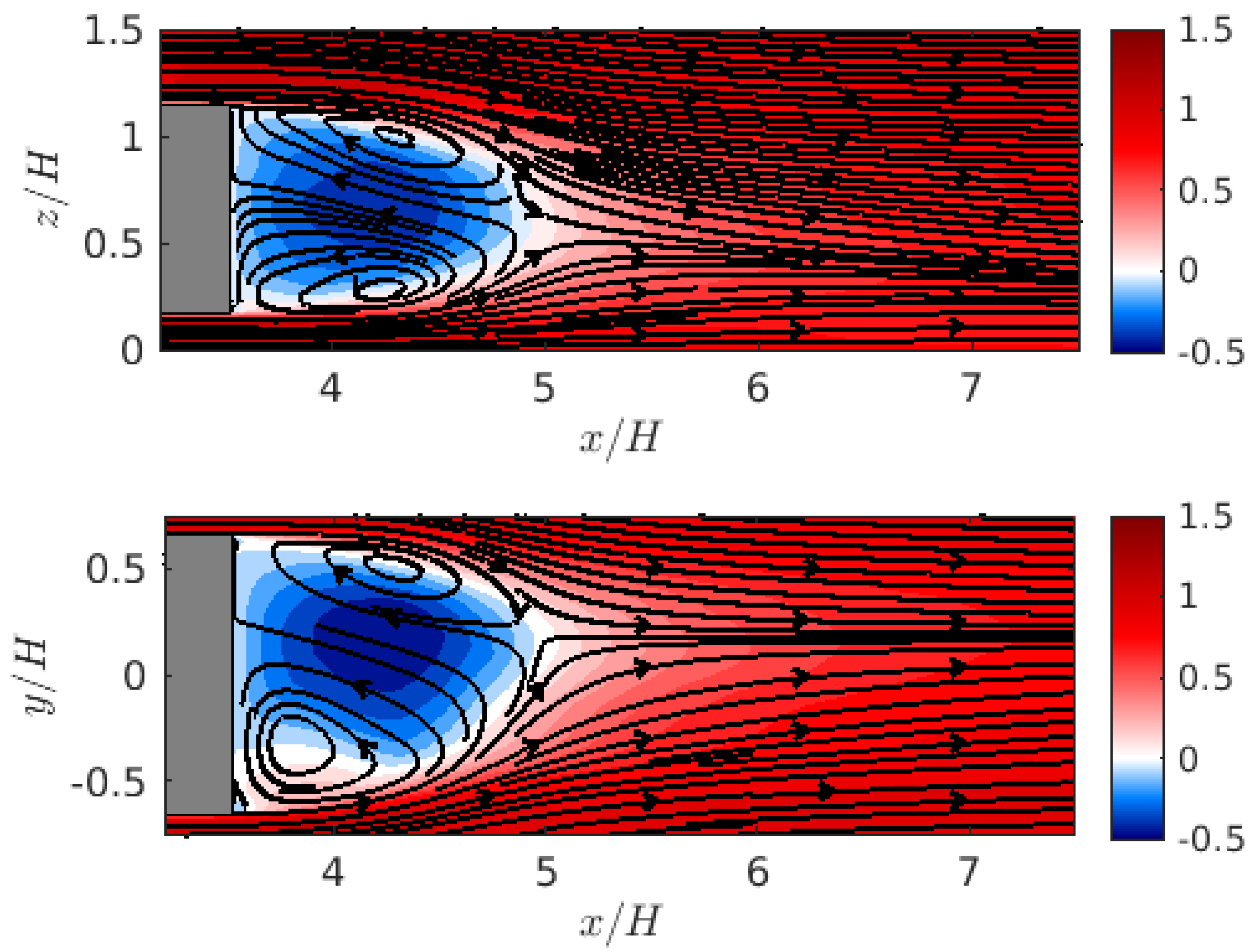
Figure 4 presents the time-averaged u-velocity and streamlines at planes: $y=0$ (center-line), $z=0.5H$ (mid-height); note that data was average over a non-dimensional time-window $T^{*}\equiv T\times U_{\infty }/H$ of $\approx 288$. The u-velocity and streamlines at the vertical plane $y=0$ show that the wake is slightly asymmetric in the vertical direction due to the ground effect. This asymmetry is evident as the near-ground recirculation bubble is different in size and shape compared to the one near the upper edge. The plane at $z=0.5H$ illustrates that the wake is also asymmetric direction, primarily due to the bi-stability phenomenon. The data suggest that the flow predominantly experiences the positive phase of bi-stability, where the wake oscillates from one side to the other with its own characteristic time scale.

The recirculating patterns observed in the vertical and spanwise directions differ due to the distinct flow topologies emerging from the upper and lower edges compared to the vertical edges. Velocity contours at both the $y=0$ and $z=0.5H$ planes indicate that the recirculation bubble extends nearly $1.5H$ downstream of the rear fascia, consistent with findings in previous studies [4,5]. Compared to the literature, particularly the works of Volpe et al. [5] and Grandemange et al. [4], the streamline pattern at the $z=0.5H$ plane exhibits pronounced asymmetry. This asymmetry suggests that the simulation predominantly captures one of the bi-stable states. The time scale of bi-stability is approximately $800\times H/U_{\infty }$ [5], requiring at least two orders of magnitude longer simulation time to capture both states, which is beyond our current hardware and data storage limits; note that the raw data stored for the results in this paper require 10 TB of storage.

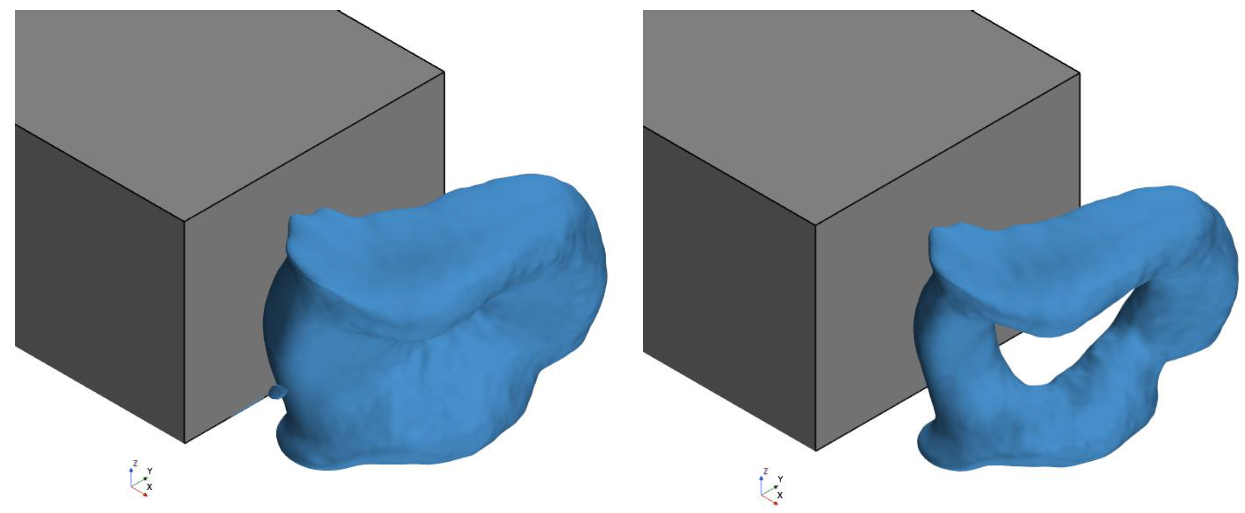
Figure 5 shows pressure iso-surfaces for $C_p=-0.355$ and $-0.375$; here, the pressure coefficient $C_p\equiv p/\left(0.5\rho U_{\infty }^2\right)$. According to the literature [7,41], the pressure iso-surfaces at these values indicate a tilted pressure torus, characteristic of the positive phase in the bi-stability phenomenon. In the negative phase, the torus would tilt in the opposite direction. During the switching phase, the asymmetrical structure of the torus disappears, and the pressure iso-surface becomes symmetric. As can be seen, the torus in this study is tilted and moving away from the right edge. Due to the short simulation time, only the positive phase is captured in this study, as reflected by the strong presence of the positive state in Figure 5.

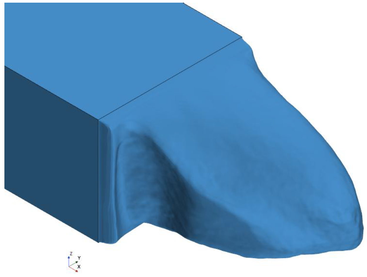
Figure 6 presents velocity iso-surfaces at $u/U_{\infty }=0.1$. The time-averaged iso-surfaces represent the general structure of the wake, which appears asymmetric, consistent with the positive phase of bi-stability discussed earlier. During right phase, wake shifts toward the right due to momentum deficiency in that side and forms more pronounce vortex shedding. The topology of the velocity iso-surfaces shows good agreement with the experimental work of Volpe et al. [5].

The flow topology and properties observed in this study show good agreement with existing literature, demonstrating that the SST-IDDES turbulence model used in the current work effectively captures the statistical properties of the flow and its complex topology. The model successfully captured the saddle points and the asymmetrical structures induced by the upper, lower, and vertical edges.

4.3. POD Analyses

Given the lack of available reference DMD data for direct validation of our modal decomposition, we adopted an indirect approach. Specifically, we compared the 2D-POD results from our studies with those reported in the literature. The use of POD for this purpose is justified, as it is a well-established technique for identifying coherent structures in fluid flows, and provides a robust basis for comparison. For that matter, a 2D-POD was applied to decompose the pressure signal on the rear fascia and the u-velocity at a plane normal to $y=0.25W$ due to the availability of reliable experimental data. The plane at $y=0.25W$ was specifically chosen instead of $y=0$ because the wake is in the positive state of bi-stability. This selection ensures that the analysis captures the relevant flow structures associated with this state. By comparing our POD results with existing literature, we ensure that the resolved flow field aligns with known flow behaviors. The alignment with established flow characteristics confirms the reliability of our data and adds to the confidence level of the subsequent analyses derived from the application of DMD for modal decomposition.

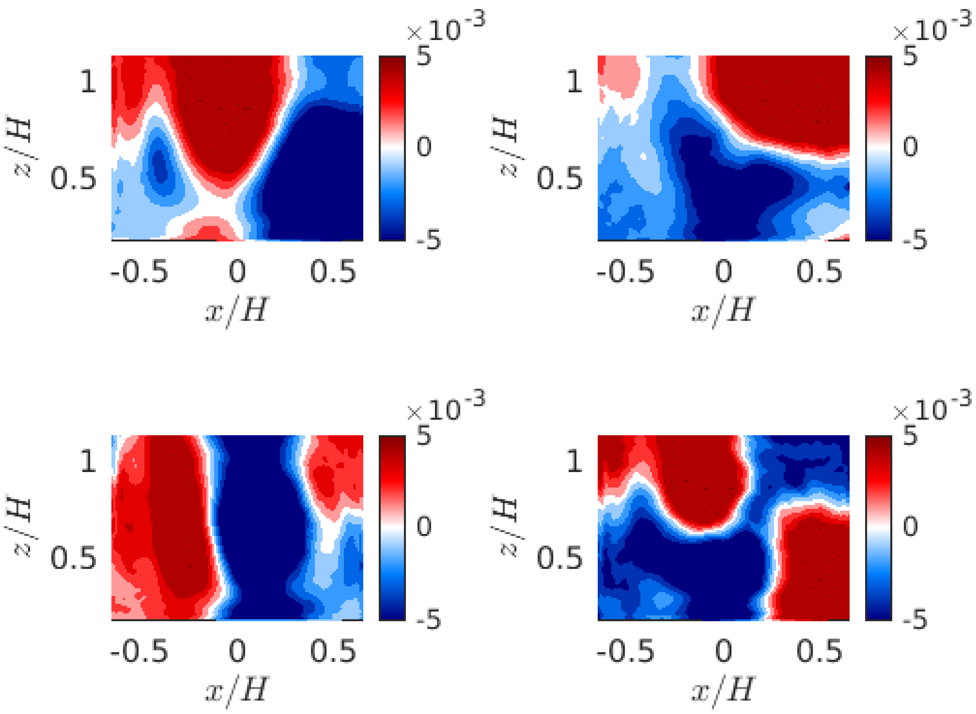
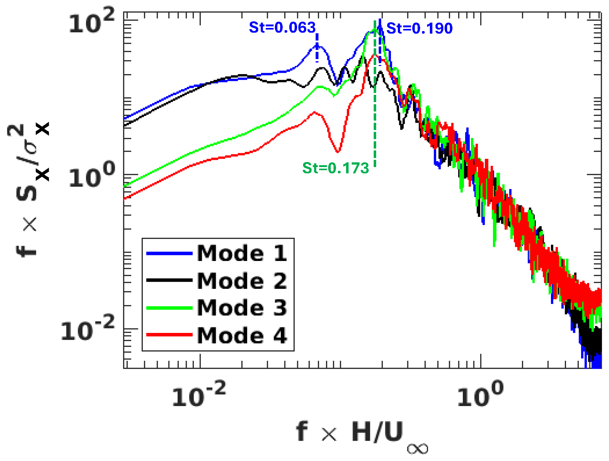
Figure 7 shows the spatial distribution of the POD mode amplitudes of the rear fascia pressure signal, while Figure 8 displays the corresponding frequency spectra for modes 1 through 4. The vertical axis in Figure 8 represents the normalized spectral amplitude, $f·S_p/{\sigma }_p^2$, where S and ${\sigma }_p^2$ denote power spectral density and the square of the variance of the signal, respectively. The subscript p indicates that these quantities are derived using the pressure signal. This normalization ensures that the spectral contributions are dimensionless and scaled relative to the total variance, facilitating a comparison of energy distribution across different frequencies. Note that in the analyses to follow, the subscripts u, v, and w will imply quantities derived from the time signals of these components of the velocity vector.

The spatial distribution of the amplitude of the first mode, shown in Figure 7 (top left), reveals alternating positive and negative regions along the spanwise direction. A similar mode shape, exhibiting symmetry-breaking structure, was also identified in Pavia et al. [43]. The frequency spectrum of this mode (see Figure 8) shows that it is dominated by low-frequency structures in the range $St\le 0.2$, where most of the energy is concentrated. The spectrum does not exhibit a distinct peak, although a gradual peak is observed at $St\approx 0.015$. Additionally, small but distinguishable peaks appear at $St=0.063$, $0.08$, and $0.13$; in subsequent discussions, these will be referred to as secondary peaks.

Like the first mode, the second mode, as shown in Figure 7 (top right), also exhibits a spatial distribution characterized by alternating positive and negative regions across the upper and lower edges, with a slight clockwise torsion shifted toward the right-hand side. Figure 8 illustrates that this mode is also dominated by low-frequency structures within $0.05\le St\le 0.2$. However, for this mode, low-frequency motions corresponding to $St\le 0.02$ have significantly lower energy contents compared to the first mode. The spectrum for mode 2 peaks at the levels of secondary peaks observed for the first mode. As noted by Pavia et al. [43], this mode is associated with a phenomenon known as “vertical symmetry breaking”.

Figure 7 (bottom left) illustrates the spatial distribution of the amplitude of the third mode, which exhibits a semi-strip pattern of alternating positive and negative regions. According to Pavia et al. [43] and Dalla et al. [23], this mode corresponds to a symmetry-preserving structure. The frequency spectrum of the third mode, in Figure 8, shows a significant reduction in the energy content of very-low-frequency motions, with a first peak at $St\approx 0.098$ and a dominant second peak at $St\approx 2.495$, which will be discussed in further detail in Section 4.4.1.

Figure 7 (bottom right) presents the spatial amplitude distribution of the fourth mode. It exhibits a cyclic pattern of alternating positive and negative amplitude regions, indicating a complex interaction of vortex shedding from the vertical and horizontal edges. The corresponding frequency spectrum shown in Figure 8 indicates that the fourth mode is dominated by motions within the range $St=0.1$ to $0.2$, with the most energetic motion at $St=0.143$ and additional peaks of similar magnitude at $St=0.13$ and $St=0.194$.

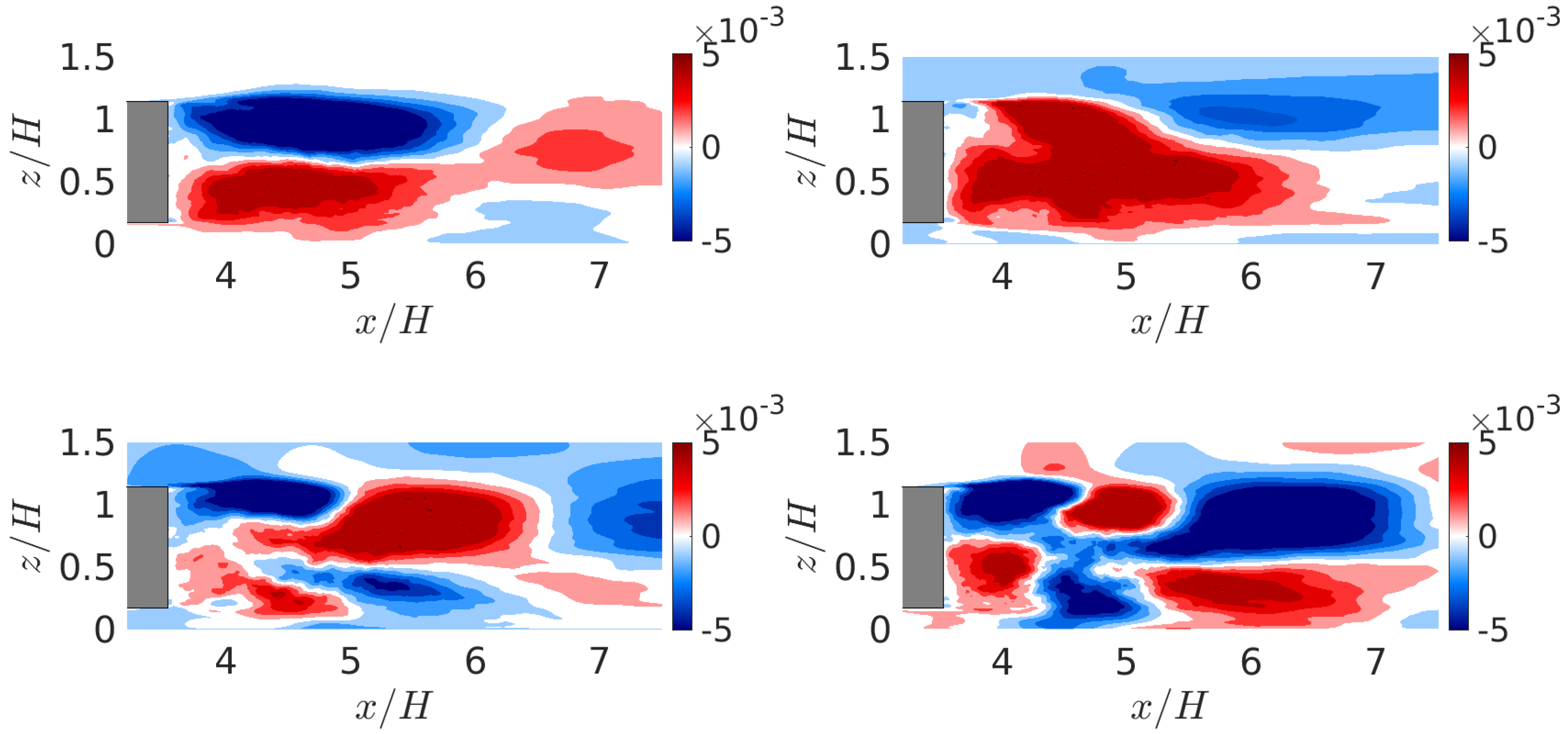
Figure 9 illustrate the spatial distribution of POD mode amplitudes for the u-velocity component within a plane normal to the y-axis at $y=0.25W$, with corresponding frequency spectra for the first four modes presented in Figure 10. The first mode’s spatial distribution, as depicted in Figure 9 (top left), reveals alternating negative and positive regions along the vertical axis, a characteristic of the symmetry-breaking structures identified by Booysen et al. [10]. This distribution signifies a momentum surplus in the lower flow region and a deficit in the upper region, indicating the absence of reflective symmetry about the horizontal mid-plane. The associated frequency spectrum, Figure 10, demonstrates that the majority of energy resides below a $St$ of 0.1, with a primary peak at $St\approx 0.063$. A secondary peak at $St\approx 0.19$ is also observed for this mode. It is noteworthy that all POD modes, with the exception of the third mode, exhibit a prominent motion at $St$ of approximately 0.19. This value, approximating 0.2, corresponds to the Strouhal number associated with large-scale wake instability in flows over bluff bodies [44].

As shown in Figure 9 (top right), the spatial amplitude distribution of the second mode exhibits a bulk region of positive values. The frequency spectrum of this mode (see Figure 10) displays a broad energy distribution up to $St\approx 0.1$, with several peaks extending to $St\approx 0.2$. The mode shape and corresponding spectrum indicate that this mode is associated with symmetry-breaking structures across the spanwise direction.

Figure 9 (bottom left) shows spatial amplitude distribution of the third mode that represents vortex shedding from the upper and lower edges of the body. The scale of vortex shedding from the upper edge is larger than that from the lower edge, contributing to the vertical asymmetry of the wake, as discussed in Section 4.2. This mode has a strong peak at $S{t}_H=0.173$ (see Figure 10), as widely reported in the literature [5,11].

The spatial amplitude distribution of the fourth mode, shown in Figure 9 (bottom right), reveals a large scale of oscillatory positive and negative regions extending from the upper and lower edges, and its amplitude increases as moves away from rear fascia. Mode pattern is similar to POD mode of u-velocity obtained by Podvin et al. [9]. The frequency spectrum of the corresponding mode, presented in Figure 10, features energy concentration in range near $St\approx 0.194$. This mode is associated with vortex shedding from the upper and lower edges, and its energy increases in far wake.

In summary, the computed POD modes in this study show good agreement with previous research in both spatial distribution of modes amplitude and temporal characteristics.

Table 3. Energy contribution of modes 1 to 4 on rear fascia and plane $y=0.25W$.

Scalar, Location	Mode 1	Mode 2	Mode 3	Mode 4
p; Rear fascia	30.1	12.1	7.8	4.6
u; $y=0.25W$	10.2	6.6	5.0	2.8

summarizes the energy content of each mode to the total energy of the corresponding field variable at relevant plane after subtracting the mean. The calculation of the energy contribution is explained in Appendix A.

4.4. DMD Analyses

This section employs Dynamic Mode Decomposition (DMD) to analyze flow dynamics and coherent structures. Initially, spectral characteristics of key DMD modes are identified, followed by an examination of their spatial amplitude distributions. Next, energy contributions of dominant structures are assessed for their aerodynamic impact and, finally, pressure–velocity DMD spectrum amplitude correlations are analyzed across frequency ranges.

4.4.1. Coherent Flow Structures

Unlike Fourier transform, DMD does not inherently order modes by frequency. Therefore, time dynamics are sorted in ascending frequency to identify and analyze key modes associated with dominant coherent structures influencing system response. Mode amplitudes are determined by the root mean square (RMS) of the time dynamics. Pressure signal amplitudes are normalized by the mean pressure mode amplitude on the Ahmed body surface, while velocity components are normalized by $N{U}_{\infty }$, where $U_{\infty }$ represents the free-stream velocity and N the number of snapshots. DMD spectra for pressure and the three velocity components are presented in Figure 11, Figure 12 and Figure 13, corresponding to planes normal to the x, y, and z axes, respectively; the locations of these planes are illustrated in Figure 3.

Figure 11, Figure 12 and Figure 13 illustrate a low-frequency range ($St<0.07$) characterized by a broadband energy distribution without distinct, well-defined peaks. The amplitude of the low-frequency range reaches its maximum at approximately $x=1.1L$ for pressure, $x=1.2L$ for the u- and v-velocity components, and $x=1.5L$ for the w-velocity. At planes normal to the y-axis, the amplitude of low-frequency structures peaks at the center-plane for all scalars except the w-velocity, which exhibits its maximum energy off-center. In the z-direction, the energy of low-frequency modes generally peaks at $z=0.75H$, except for the v-velocity, which reaches its maximum at $z=0.5H$. The amplitude decreases from body to far wake as shown in Figure 11a,b and from the center toward the upper/lower and side edges; see Figure 12a,b and Figure 13a,b.

DMD spectra also reveal the presence of a bubble-pumping mode in several planes. As shown in Figure 11a, pressure exhibits a peak at $St\approx 0.072$ at planes from $x=1.2$ to $2.5L$, which its amplitude decreases further downstream. The location of the bubble-pumping mode aligns with the findings of Volpe et al. [5]. For all three velocity components, no predominant peaks corresponding to bubble-pumping modes are observed in planes normal to the x-axis; see Figure 11b,c.

In Figure 12a–d, the mode at $St\approx 0.072$ for pressure shows strong peaks at planes $y=0$ and $0.25W$, while the w-velocity exhibits a peak at $0.25W$. However, for u-velocity, no significant peaks corresponding to bubble-pumping modes are detected.

The presence of bubble-pumping modes extends to planes normal to the z-axis. The pressure signal exhibits peaks near $St\approx 0.07-0.08$ at ALL planes except $z=0$; see Figure 13a. Additionally, Figure 13b,d shows that u and w-velocity exhibit distinct peaks at $St\approx 0.072$ at $z=0.75H$. In general, the amplitude of the bubble-pumping dynamics reaches its maximum around $z=0.75H$.

In the pressure signal at planes normal to the x, y, and z-axes, shown in Figure 11a, Figure 12a and Figure 13a, one of the most prominent peaks occurs at $St\approx 0.130$ at $x=1.2L$, $1.5L$, $y=0$, $0.25W$, and $z=0.25H$. Booysen et al. [10] identified this mode as vortex shedding originating from the lateral edges and located it at $x=1.3H$ using hot-wire measurements of the u-velocity. However, in this study, u-velocity does not exhibit a dominant mode at $St\approx 0.130$, as shown in Figure 11b, Figure 12b, and Figure 13b. Overall, this mode reaches its highest amplitude levels at $x=1.2L$, $y=0.25W$, and $z=0.25H$ in the pressure signal.

Figure 11b,c shows that the u and v-velocity components at planes $x=1.5L$, $2L$, and $2.5L$ exhibit a notable peak at $St\approx 0.166$. Additionally, for pressure at $y=0.5W$, a mode at $St\approx 0.151$ is observed; see Figure 12a. This mode also appears as a minor peak for u-velocity at $y=0$, as shown in Figure 12b. These modes are associated with vortex shedding emanating from the upper and lower edges of the body and significantly impact lift forces [7]. The maximum amplitude of mode at $St=0.166$ is located at $x=1.5L$, $y=0.25L$, and $z=0.75H$.

A notable vortex-shedding structure, known as Bernard–Von Kármán vortex shedding, occurs in the far wake within shear layers. Lahaye et al. [14] reported that the peak associated with this structure strengthens as the measurement probe moves further from the base, classifying it as a far-wake phenomenon. Barros et al. [11] identified vortex shedding from the top and bottom edges at $St\approx 0.2$, while Podvin et al. [9] found a characteristic frequency range of $0.19<St<0.24$, corresponding to vortex shedding and pairing in the far wake.

Consistent with these findings, we observed a peak at $St\approx 0.194$ across all four variables (p, u, v, and w) in the DMD spectra at x-planes downstream of $x=1.5L$; see Figure 11a–d. The DMD spectra at y-planes in Figure 12a–d show that far-wake vortex shedding reaches its highest peak at $y=0.25W$. However, at z-planes, the peak varies among variables: it occurs at $z=0.75H$ for pressure and u-velocity, as shown in Figure 13a,b, while for v and w-velocity components, it appears at $z=0.5H$; see Figure 13c,d.

The DMD spectra of y-planes reveal a dominant peak at the high frequency of $St\approx 2.495$. This peak appears as one of the most energetic modes for pressure and v-velocity at $y=0.5W$ shown in Figure 13a,c. It also appears with weaker amplitude across all four variables at $x=1.1L$ and at $z=0$ and $1H$ shown in Figure 11a–d and Figure 13a–d, respectively.

Lahaye et al. [14] observed dominant oscillatory structures in the $St\approx$ 1.5–4.5 range, linking them to Kelvin–Helmholtz instabilities in shear layers. Liu et al. [45] reported high-frequency structures near $St\approx 2.12$, equivalent to $St\approx 0.58$ relative to the height, attributing them to vortex shedding from upstream struts.

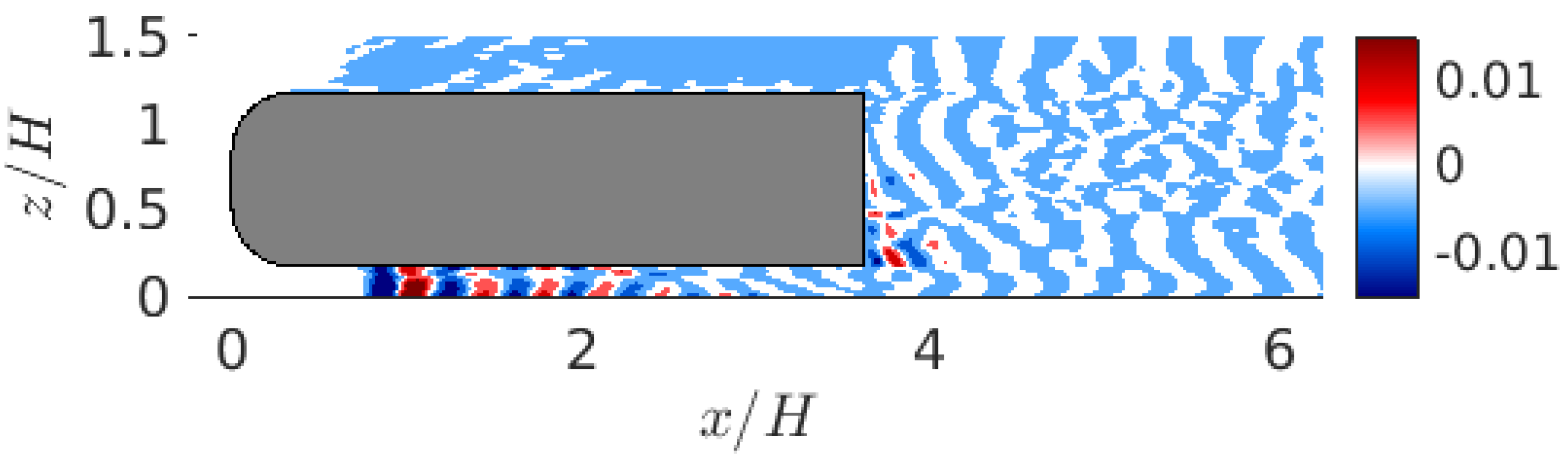
To determine the origin of this mode, we present the spatial amplitude distribution of the mode at $St\approx 2.495$ for u-velocity at $y=0.5W$ in Figure 14. This plane was selected as it is closer to the upstream struts. The results reveal small-scale vortex shedding originating from the upstream struts, consistent with the findings of Liu et al. [45]. However, its peak value is nearly five times higher than that reported in their study, possibly indicating that this mode represents a harmonic of a component with $S{t}_H=0.5$.

To investigate the relationship between flow dynamics in the near and far wake and the body forces on the Ahmed body, we analyzed the DMD spectrum of pressure on the rear fascia, which has the highest contribution to total drag.

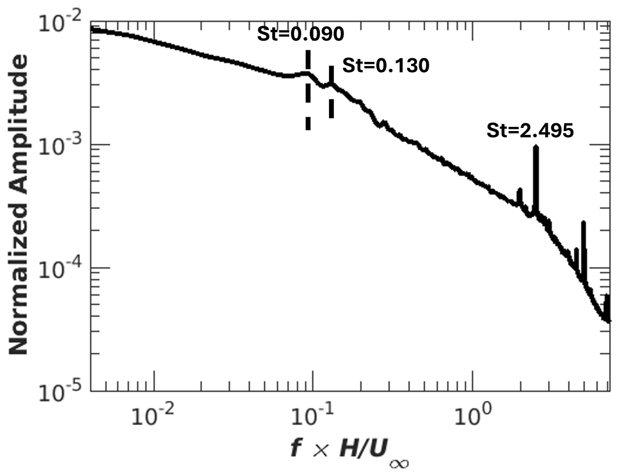
Figure 15 presents the DMD spectrum of the pressure signal. Symmetry breaking in the range of $St<0.07$ accounts for a significant level of energy without a dominant peak. The first distinct peak appears at $St\approx 0.09$, associated with symmetry-preserving structures, followed by a secondary peak at $St\approx 0.130$ linked to lateral-edge vortex shedding. A high-frequency peak at $St\approx 2.495$ corresponds to vortex shedding from upstream struts. These results indicate that base drag is primarily influenced by symmetry breaking, symmetry preserving, bubble pumping, and vortex shedding from lateral edges.

An important observation from the DMD spectral analysis is that pressure and velocity components do not always exhibit synchronized modal behavior. In several cases, a coherent structure associated with a specific frequency shows a strong spectral peak in pressure, while the corresponding velocity components display a much weaker or no response, and vice versa. Additionally, the spatial location at which a given mode reaches its maximum amplitude sometimes differs between pressure and velocity fields. This highlights the importance of multi-variable modal analysis in uncovering a more complete picture of wake dynamics, as relying on a single scalar may overlook or misrepresent key energetic structures.

4.4.2. Spatial Structures of DMD Modes

To gain deeper insight into the spatial evolution of dominant flow structures, we analyze the spatial distributions of selected DMD mode amplitudes. Understanding these spatial characteristics helps identify regions of high energy concentration and their interaction with the wake dynamics. Among the observed modes, four modes (quasi-steady, $St\approx 0.072$, $St\approx 0.166$, and $St\approx 0.194$) have been chosen for detailed examination due to their significance and recurrence across different planes and field variables. All present modes in this section are extracted from u-velocity at plane $y=0.25W$.

Figure 16 shows the spatial distribution of the DMD mode corresponding to a quasi-steady structure at $St\approx 0.004$. This mode is the first neighboring mode after the mean mode and exhibits large-scale vertical oscillations. It is associated with symmetry breaking in the vertical direction, with a length scale aligning with the wake’s characteristic length. The amplitude of spatial mode reaches to maximum at $x=4.1H$ and $z=0.32H$ (from lower edge). Its spatial pattern closely resembles POD Mode 1, as shown in Figure 9. In this plane, other symmetry-breaking structures frequently appear among the first twenty energetic modes, including vertical symmetry-breaking modes at $St\approx 0.025$, $0.036$, and $0.054$, and lateral modes at $St\approx 0.014$, $0.018$, and $0.039$.

Figure 17 illustrates the spatial amplitude distribution of the DMD mode at $St=0.072$, associated with the bubble-pumping structure. The alternating positive and negative regions indicate inflation and deflation in the shear layers, with energy concentration near upper edge, and its maximum occurs at $x=4.3H$ and $z=0.84H$ (from lower edge). This DMD mode exhibits considerable similarity in spatial pattern to the POD mode computed by Podvin et al. [9].

The spatial amplitude distribution of the DMD mode at $St\approx 0.166$ is shown in Figure 18. Its spatial pattern represents vortex shedding originating from the upper and lower edges, with higher energy concentrated near the upper edge and a slight downwash tendency with a highest amplitude near $x=5.6H$ and $z=0.71H$. This pattern closely resembles the POD mode shape obtained in Section 4.3, as shown in Figure 9. The premultiplied frequency of the corresponding POD mode is $St=0.173$.

The spatial distribution of the DMD mode amplitude at $St\approx 0.194$ is shown in Figure 19. Its spatial mode shape illustrates the interaction between vortex shedding from the top and bottom edges, with nearly equal amplitude along both edges. This mode shares some similarities with the fourth POD mode, as shown in Figure 9. However, unlike the fourth POD mode, its energy dissipates as it moves away from the base, and its length scale is larger in the near wake, whereas the fourth POD mode exhibits a larger scale in the far wake. The mode amplitude peaks near $x=5H$ and $z=0.82H$.

Another important observation is that, unlike POD, DMD can identify specific regions where each mode with individual frequency exerts its influence. However, unlike POD, where spatial modes are orthogonal, DMD modes are not and may exhibit scatter and irregular spatial patterns and are more subject to mode contamination and numerical sensitivity.

4.4.3. Energy Contribution of Dynamic Structures Across Distinct Frequency Regimes

Oscillatory frequency-based flow regime classification offers insights into control mechanisms, though few studies employ this approach. For example, Chovet et al. [46] identified low-frequency ($St\le 0.15$) and moderate-frequency ($St>0.15$) regimes. However, this classification may be inadequate due to the distinct mechanisms governing symmetry breaking, bubble pumping, and edge-induced vortex shedding. Thus, this section examines the energy contribution of dynamic structures within $St\le 0.2$, dividing it into three regimes: (a) symmetry breaking (SB) for $St\le 0.07$, (b) bubble pumping (BP) for $0.07\le St\le 0.1$, and (c) low-frequency vortex shedding (VS) for $0.1\le St\le 0.2$. Energy contributions are assessed on three planes normal to the x, y, and z-axes (Figure 3). It is worth noting that BP may overlap with SB and VS, as some structures from these frequency regimes appear within SB. However, observations from the spatial mode amplitude distribution in Section 4.4.2 indicate that the bubble-pumping mode at $St\approx 0.072$ typically emerges as the dominant mode in this frequency range, except for a structure exhibiting features of symmetry preservation observed at $St\approx 0.09$. The calculation methodology for energy contribution from reconstructed flow fields is detailed in Appendix A.

Figure 20a–d depicts the energy contribution of pressure, and three velocity components (u, v, w) at x-planes ranging from $1.1L$ to $2.5L$. Notably, the energy contribution of SB components consistently decreases with increasing distance from the body for all four variables, reaching a minimum at $2.5L$. A similar, albeit slower, decreasing trend is observed for BP structures. Conversely, the energy content of VS structures increases along the streamwise direction for pressure and u-velocity, while remaining relatively constant for v and w-velocity components. Initially, SB structures exhibit the highest energy content at $1.1L$; however, further downstream, VS structures dominate, particularly at $2.5L$; see Figure 20a–d. Among the variables, u-velocity demonstrates the highest energy concentration. The transition point, where SB and VS energy levels intersect, occurs at $1.2L$ for pressure, v-velocity, and w-velocity, near the center of the recirculation bubbles. It can be seen in Figure 20b that for u-velocity, this transition occurs at $1.4L$, near the saddle point.

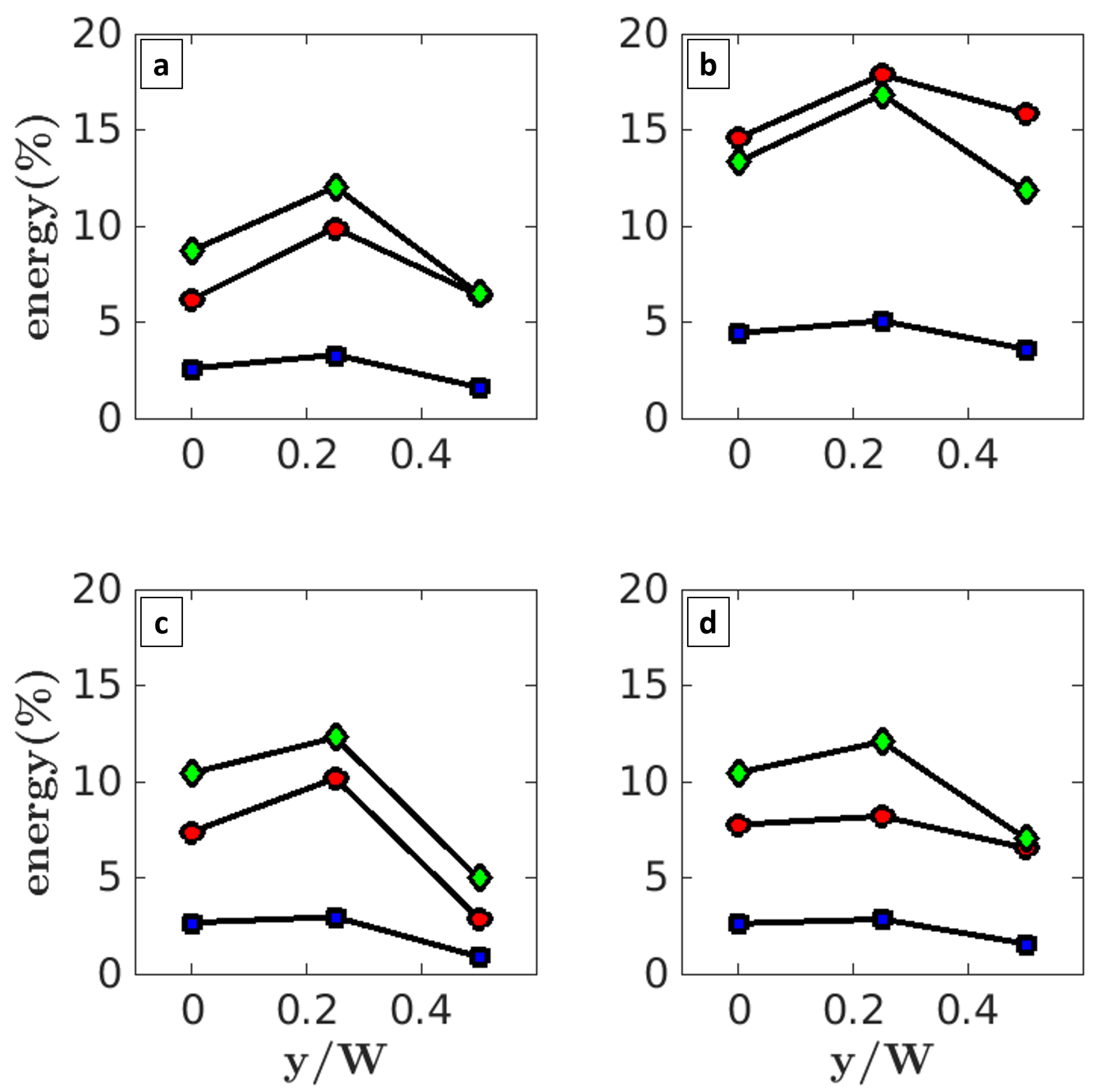
The energy contributions of SB, BP, and VS structures are analyzed at planes $y=0$, $0.25W$, and $0.5W$, as shown in Figure 21a–d. All four variables reach their highest energy contribution at $y=0.25W$, a quarter width from the center-line and outer edges. This concentration likely reflects the dominance of the positive state in bi-stability. Figure 21b illustrates that among the four variables and across the x-planes, u-velocity holds the highest energy concentration. SB structures reach a peak energy contribution of nearly 20% at $y=0.25W$, while VS structures contribute slightly less, and BP remains less than 5%. The energy content of p, v, and w are approximately the same across all three flow regimes, as shown in Figure 21c,d.

Energy contributions of three dynamic regimes were analyzed at planes normal to the z-axis, spanning 0 to $1H$, as depicted in Figure 22a–d. Consistent with observations in x- and y-planes, u-velocity exhibits the highest energy concentration, notably for SB and VS regimes; see Figure 22b. The SB energy contribution increases steadily from the lower to the upper edge, peaking near 20% at $1H$. VS follows a similar trend, peaking earlier at $0.75H$, while BP displays a gradual increase from 0 to $1H$, with an approximate 2% overall rise. For pressure (p) and velocity components (v, w) as shown in Figure 22a,c,d, energy trends fluctuate around the central plane. Pressure exhibits SB peaks at $0.25H$, VS at $0.75H$, and BP at $0.5H$. In v-velocity, VS dominates, with all three regimes peaking at $0.5H$, a trend similarly observed in w-velocity, except SB and BP peak at $0.75H$. Overall, the majority of energy is concentrated within the range $0.25\le z\le 0.75$, towards the central plane.

The energy contributions of three dynamic regimes to pressure on the rear fascia were analyzed. The symmetry-breaking component contributes approximately 44.6% of the total energy, followed by vortex shedding at 20% and bubble pumping at 10%. These contributions significantly surpass those observed in the x-, y-, and z-planes. For instance, at the plane nearest to the rear fascia ($x=1.1L$), symmetry breaking, bubble pumping, and vortex shedding contribute 18%, 4%, and 8%, respectively. These findings underscore the potential for substantial base drag reduction through effective control of all three regimes, with particular emphasis on symmetry breaking.

To develop effective and targeted flow-control strategies, it is essential to understand where and how different coherent structures dominate the wake. Mechanisms such as symmetry breaking, bubble pumping, and vortex shedding arise from distinct physical instabilities and require different control approaches. To address this, we combined spectral peak locations from DMD time dynamics with spatial mode distributions and cross-validated them using energy contribution trends across planes and variables. The resulting energy distribution map (Figure 23) identifies regions of maximum influence for each mechanism, serving as a practical guide for designing location-specific and mechanism-aware control strategies.

The energy distribution map reveals several important spatial characteristics of dominant coherent structures. SB is concentrated near the rear fascia, with its maximum vertical symmetry breaking located asymmetrically between the upper and lower edges. This suggests that it is not evenly distributed across the vertical plane, implying that symmetric control strategies—such as uniform forcing at the top and bottom edges—may not be effective. Instead, targeted manipulation near the upper/lower regions may yield greater impact. Similarly, BP region extends further downstream and upward, with its energy maximum skewed toward the upper recirculation for $St=0.072$. Lateral vortex shedding shows a localized peak near the lower corners and center of lower recirculation bubble, while upper-edge and far-wake vortex-shedding structures appear predominantly in the upper shear layer and further downstream. These spatial differences highlight that each mechanism occupies a distinct region and follows a unique energy footprint. Therefore, the flow-control approach should not only match the dominant frequency of the structure but also be spatially aligned with its region of influence. The map thus provides practical guidance for optimizing control placement and strategy, especially in cases where the energy distribution is not symmetric.

4.4.4. Correlation of Field Variables

A complete understanding of the interactions among flow structures in near- and far-wake regions requires an analysis of the correlation between the pressure and velocity components. For instance, Barros et al. [11] demonstrated that an increase in correlation between base pressure and velocity in the near wake can reduce base pressure by up to 25%, leading to an increase in base drag. To this end, we quantified the correlation between these variables across distinct frequency ranges only in range of $0\le St\le 0.2$ to match with flow regimes in Section 4.4.3 by computing the Pearson correlation of Dynamic Mode Decomposition (DMD) spectral amplitudes, which were previously sorted in ascending frequency order. This approach allows us to discern how fluctuations in pressure relate to corresponding variations in velocity components at specific frequencies, thereby illuminating the dynamic coupling between these flow properties. Specifically, the Pearson correlation coefficient, calculated from the DMD spectral amplitudes, provides a measure of the linear relationship between pressure and each velocity component at each frequency. The mathematical formulation of the Pearson correlation employed in this study, including the precise equations used for its computation, is detailed in Appendix B, providing a transparent and reproducible methodology.

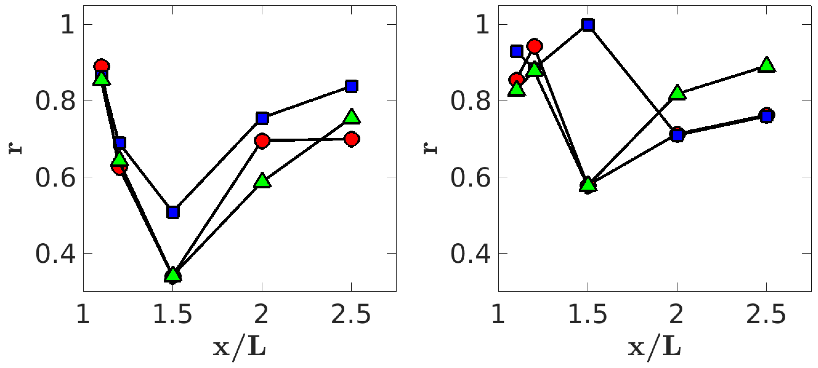
Figure 24 presents correlation values obtained from data collected on x-planes. The pressure–velocity correlations, shown in Figure 24-left, are highest at $x=1.1L$, decrease until $x=1.5L$, and then gradually recover up to $x=2.5L$. According to Podvin et al. [47], pressure and velocity fields exhibit strong correlation in the near wake. This strong correlation near the rear fascia likely plays a significant role in the formation of symmetry-breaking structures, while its recovery in the far wake may contribute to the onset of far-wake vortex shedding.

Velocity–velocity correlations in Figure 24-right indicate that $(u,v)$ and $(v,w)$ exhibit the highest correlation at $x=1.2L$, while $(u,w)$ peaks at $x=1.5L$. The shift in velocity component correlations from $x=1.1L$ to $x=1.2L$ and $x=1.5L$, compared to pressure–velocity correlations, suggests their role in the formation of vortex-shedding structures. Their DMD spectra, as shown in Section 4.4.1 in Figure 11c,d, exhibit weak peaks at $x=1.2L$. Beyond this location, vortex-shedding structures at $St\approx 0.163$ and $0.914$ become more pronounced in the range $1.5\le x\le 2.5$, with the highest energy level at $x=1.5L$. The strong correlation observed at $x=1.5L$ for $(u,w)$ may indicate the key role of this velocity pair in the development of vortex shedding.

Figure 25 presents correlation values along y-planes. Correlation coefficients reach their highest values at the quarter-span plane ($y=0.25W$) and their lowest at the side plane for both pressure–velocity (Figure 25-left) and velocity–velocity (Figure 25-right) correlations, except for $(u,v)$, which peaks at $y=0$. The strong correlation at $y=0.25W$ suggests that symmetry-breaking, bubble-pumping, and vortex-shedding structures predominantly couple on the right half of the body in the positive state of bi-stability. The Figure 12a–d also prove that plane $0.25W$ has the highest energy content with the most appearance of coherent structures.

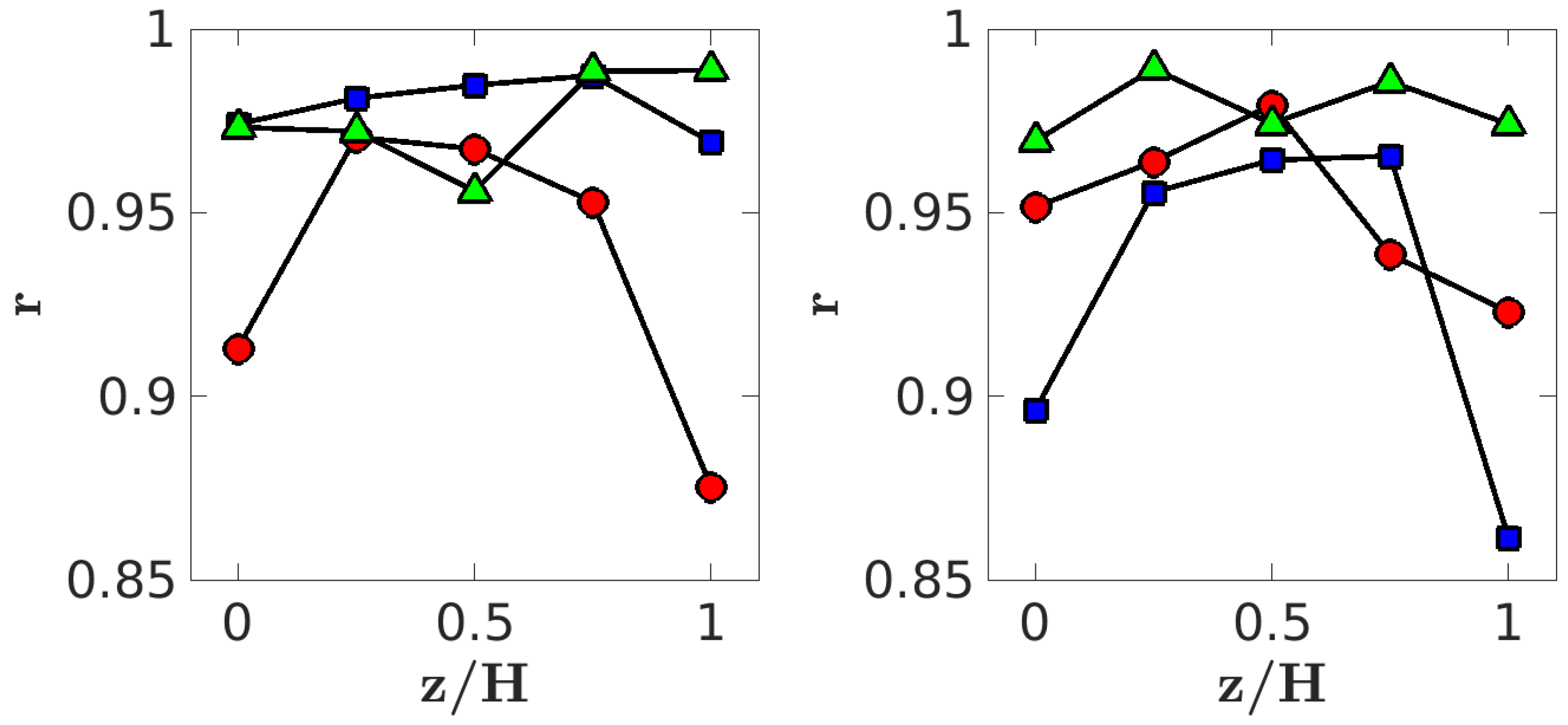
Figure 26 presents quantified correlation values along z-planes. Pressure–velocity correlations are high near the center plane ($z=0.5H$) and reach their highest values at $z=0.25H$ for $(p,u)$ and $z=0.75H$ for $(p,v)$ and $(p,w)$, as shown in Figure 26-left. The velocity–velocity correlations (Figure 26, right) exhibit a distinct spatial pattern, with maximum correlation values varying across the vertical direction. Specifically, the $(u,v)$ pair peaks at $z=0.5H$, $(v,w)$ reaches its maximum at $z=0.75H$, and $(u,w)$ at $z=0.25H$. In general, the maximum correlation tends to be off-center, leaning toward either the upper or lower edge of the wake.

As seen in the energy distribution map (Figure 23), the maximum correlation of all pressure–velocity pairs occurs within the SB region, highlighting the key role of pressure–velocity coupling in sustaining and amplifying symmetry-breaking dynamics. Additionally, the locations of peak energy associated with vortex shedding from the upper edge and far-wake correlate well with regions where the $(u,v)$ correlation reaches its maximum. This suggests that the direction of dominant velocity fluctuations in the x–y plane—derived from the corresponding DMD mode—may provide guidance on where and how to apply external forcing, such as jet injection, to influence these structures. Finally, the region of maximum energy associated with lateral vortex shedding coincides with the location of maximum correlation in the $(v,w)$ pair, further supporting the relationship between energy content and cross-component coupling in the wake.

5. Conclusions

In this study, we analyzed the drag force, mean flow topology, and modal decomposition using POD and DMD for flow past an Ahmed body at a high Reynolds number ($R{e}_H=7.7\times {10}^5$). DMD mode shapes, their temporal dynamics, and the energy distribution of dynamic structures were examined in both spatial and temporal domains. Correlations between field variables were analyzed using the Pearson method applied to the DMD frequency spectra. All analyses were conducted for pressure, and the three velocity components across planes normal to the x, y, and z axes. The following conclusions summarize the key insights gained from these analyses.

The drag analysis revealed that pressure drag accounts for 85% of the total drag, with base drag contributing 72%, aligning well with previous studies. The mean flow structure exhibited asymmetrical recirculation bubbles in vertical and lateral directions.

Through POD decomposition, dominant flow structures and their spectral characteristics were identified. The leading POD mode captured large-scale coherent structures, significantly contributing to energy distribution. The computed modes across the rear fascia and plane $y=0.25W$ captured symmetry-breaking and -preserving structures, as well as lateral, upper/lower, and far-wake vortex shedding. The results validated the collected numerical data before applying DMD for further modal decomposition, ensuring the robustness of the analysis.

DMD analysis provided insights into the spatial and temporal evolution of wake structures by isolating individual frequency oscillatory components. Several dominant mechanisms were identified, including symmetry breaking at $St<0.07$, bubble pumping at $St=0.072$, and vortex shedding from lateral, upper, and lower edges at $St\approx 0.132$, 0.151, and 0.166. A far-wake vortex-shedding mode at $St=0.194$ emerged downstream of $x=1.5L$, reinforcing previous observations of wake instabilities. Additionally, a high-frequency mode at $St=2.495$ was linked to vortex shedding from upstream struts. The DMD spectral analysis also revealed that pressure and velocity components do not always exhibit synchronized modal behavior. In some cases, strong pressure peaks appeared without corresponding velocity responses and vice versa, underlining the need for multi-variable analysis to fully capture wake dynamics.

The energy contribution analysis categorized the wake into three regimes: symmetry breaking (SB) in the range $0\le St<0.07$, bubble pumping (BP) for $0.07<St\le 0.1$, and vortex shedding (VS) for $0.1<St\le 0.2$. SB and BP exhibited the highest energy at $x=1.1L$, $y=0.25W$, and $0.25<z/H\le 0.75$. However, the energy gradient of SB was higher than BP. Although BP energy declined as it moved away from the rear fascia, it did so at a slower rate than SB. In contrast, for vortex shedding, the highest energy contribution was observed at $2.5L$, $0.25W$, $0.75H$ for pressure and u-velocity, and at $1.1L$, $0.25W$, $0.5H$ for v-velocity and w-velocity. These findings suggest that pressure and u-velocity play a more significant role in far-wake vortex shedding, while v-velocity and w-velocity contribute to lateral and upper/lower vortex shedding in the near wake. The energy contribution of the pressure signal on the rear fascia is 44.6%, 10%, and 20% for SB, BP, and VS, respectively. This indicates that the dominant mechanism influencing body forces on the rear fascia is SB, followed by VS and BP. The primary vortex shedding on the rear fascia occurs at $St=0.13$, corresponding to vortex shedding from the lateral edges. To visualize how these mechanisms are distributed across the wake, we introduced a spatially resolved energy map highlighting the dominant regions of SB, BP, and VS. This map, developed from DMD amplitude peaks and energy trends, shows that coherent structures occupy distinct spatial zones. Specifically, the maximum energy of vertical symmetry breaking occurs near the rear fascia and is vertically skewed toward the upper/lower edges; bubble pumping at $St=0.072$ reaches its peak around $x=4.35H$ and $z=0.75H$ near upper recirculation bubble; and upper edge and far-wake vortex exhibit maximum energy further downstream around $x=5.43H$ and $z=0.75H$, whereas lateral vortex shedding peaks at $x=4.35H$ and $z=0.25H$ in near-wake region. The map also reveals significant asymmetry in energy distribution, indicating that symmetric control strategies may not be cost-effective in influencing dominant flow features.

The linear correlation analysis of DMD spectra provided further insights into the interactions between pressure and velocity components. Pressure–velocity correlations were strongest at $1.1L$, $0.25W$, $0.25\le z/H\le 0.75$, near the rear fascia. After $x=1.1L$, correlation values decreased until $x=1.5L$ before gradually recovering up to $x=2.5L$. The coupling of pressure and velocity components plays a key role in forming symmetry-breaking and bubble-pumping structures, while its recovery in the far wake likely contributes to far-wake vortex shedding. The correlations of $(u,v)$ and $(v,w)$ were strongest at $1.2L$, $0.25W$, $0.25\le z/H\le 0.5$, near the lower recirculation and ground, suggesting their influence in forming vortex shedding from the lower and lateral edges. The $(u,w)$ correlation peaked at $1.5L$, $0.25W$, $0.25\le z/H\le 0.75$, located downstream of the saddle point near the upper edge of the Ahmed body. The coupling of u and w likely plays a key role in amplifying vortex shedding from the upper edge and its pairing with other vortex-shedding structures in the far wake. Notably, the wake in this study exhibits a positive state of bi-stability, which dominates energy distribution and variable correlation in the spanwise direction, toward the right edge. Furthermore, we observed that each correlation peak often coincided with the region of maximum energy for the associated flow mechanism. For example, $(u,v)$ correlation aligns with upper-edge and far-wake shedding zones, while $(v,w)$ peaks within lateral shedding regions. These spatial overlaps provide useful guidance for placing actuators and selecting appropriate control directions.

The findings of this study provide a detailed characterization of wake dynamics, highlighting the temporal evolution, spatial distribution, and energy contributions of dominant flow structures. These insights can support the development of passive and active flow-control strategies to mitigate drag and enhance aerodynamic performance of road vehicle. By integrating frequency-based mode classification, energy mapping, and cross-variable correlation analyses, this study offers a unified spatiotemporal perspective of wake behavior. Such insight is crucial for designing mechanism-specific, spatially localized control strategies that maximize aerodynamic efficiency while minimizing control effort.