Developing an Algorithm Limiting the Longitudinal Acceleration of an Electric Vehicle

Abstract

The electric traction drive is increasingly being applied as a device providing traction force on driving wheels. This is due to its reliable torque transmission to the driving wheels, step-less regulation of the traction force on the driving wheels depending on the driving conditions, and increased design capabilities. In terms of power, the electric traction drive has maximum torque at low speeds, which internal combustion engines lack. This property of the electric drive is not applied in urban vehicles, as not all passengers are comfortable with intensive acceleration. In modern vehicles with an electric traction drive, the maximum acceleration can be limited by software, which is the focus of this study. This paper aims to develop an algorithm capable of recognizing when the permissible longitudinal acceleration exceeds the limit and generating an action to maintain the acceptable acceleration level. The electric traction drive of a large-class electric bus was used as a control object. An algorithm and a control law are hereby developed, which reduce longitudinal acceleration using PI control. Both simulation modeling and full-scale tests on the electric bus were carried out to evaluate the performance and efficiency of the algorithm. In this paper, the authors also introduce the cumulative velocity concept and prove the operability and efficiency of the developed method.

1. Introduction

Electric traction drive vehicles are increasingly being introduced into service. These are rail-less vehicles, including electric cars, electric buses, and vehicles with hybrid traction systems. The traction electric drive is widely used due to its capability of achieving highly efficient high-power transmission to the driving wheels at a wide range of speeds (up to 12,000 rpm), step-less regulation of the traction force on the driving wheels, and energy recovery at decreasing speed [1]. In addition, the traction electric drive can develop maximum torque at low speeds (less than 500 rpm). This property improves the acceleration performance of light sports cars, since, for them, the maximum acceleration is an important parameter. However, for electric buses or trolleybuses, intense acceleration must be limited for the sake of comfort and safety.

Hence, there is a need to limit the maximum acceleration of electric buses. Moreover, the shock loads in the drive’s mechanical elements, especially the gears, should be limited both upon electric motor start-up and during motion. Considering that electric buses are operated in urban traffic, the acceleration of the vehicle, despite restrictions, should be acceptable, based on the values obtained in Refs. [2,3]. According to [4,5], the longitudinal acceleration in urban passenger electric transport should not exceed 1.5 m/s², which, taking into account Refs. [2,6,7], is not only acceptable for traffic but also quite comfortable for passengers.

As part of the development of traction electric drive control systems, the “KAMAZ” Innovation Center developed a system for limiting longitudinal acceleration. Thus, this paper aims to set out the laws and algorithms for said control system and introduce the efficiency evaluation criterion, for later application to the vehicle.

2. Derivation of the Longitudinal Acceleration Limiter Controller Equation

The following assumptions were made in developing the longitudinal acceleration limiting control law and algorithm:

• The acceleration of the vehicle while traveling forward is considered;
• The vehicle is travelling on a flat horizontal surface;
• The algorithm that calculates the control action operates when excessive acceleration is detected.

The longitudinal acceleration signal can be obtained from an inertial sensor [8] or by differentiating the angular velocity of the driving wheels and then filtering the signal.

The following is the equation of rectilinear motion during acceleration [9,10]:

$$m{\displaystyle \frac{d{v}_x}{dt}}=F_{tr}-F_f-F_w;$$

(1)

where

• $v_x$—longitudinal speed of the wheeled vehicle, m/s;
• $m$—vehicle mass, kg;
• $F_{tr}$—traction force of driving wheels, N;
• $F_f$—rolling resistance force of all wheels, N;
• $F_w$—aerodynamic drag force, N.

The phase variable based on which the traction drive torque is controlled is the difference between the permissible acceleration $a_{per}$ and the actual $a_{xact}$:

$$∆a_x\left(t\right)=a_{xact}\left(t\right)-a_{per}.$$

(2)

When designing an optimal controller, it is necessary to determine normal system operation, or, in this case, the permitted acceleration for the vehicle. When in the normal system operation mode, the vehicle acceleration is less than or equal to the permitted value. That is, the following conditions are fulfilled:

$$a_{xact}\le a_{per}or∆a_x\le 0.$$

(3)

Then, we can assume that, when the acceleration is above the limit (the initial moment of time), $∆a_x\left(0\right)>0$, and, after some time (at an infinite moment of time), $∆a_x\left(\mathrm{\infty }\right)\le 0$, i.e., the regulator strives to ensure asymptotic stability, $∆a_x=∆{\dot{v}}_x\to 0$. At the same time, the controller tends to maintain the actual velocity within the allowable acceleration; that is, the actual velocity will tend to the velocity at the allowable acceleration $∆v_x\to 0$:

$$∆v_x\left(t\right)=v_{xact}\left(t\right)-v_{per}\left(t\right).$$

(4)

In other words, the controller aims to ensure the equi-accelerated motion of the controlled object. The meaning of the above conclusions is explained in Figure 1, showing the velocities (Figure 1a) and accelerations (Figure 1b) without (red graphs) and with (green graphs) the acceleration limitation.

Let us represent the phase variables as $x_1=∆s_x$, ${\dot{x}}_1=x_2=∆v_x$ and write the equation of state in terms of perturbed motion, as follows:

$$\left\{\begin{array}{c}{\dot{x}}_1=x_2;\\ {\dot{x}}_2=-{\displaystyle \frac{1}{m}}\mathit{U},\end{array}\right.$$

(5)

where $\mathit{U}$ is the principal vector of the control action. In turn, the main vector of the control action $\mathit{U}$ is calculated by the following formula:

$$\mathit{U}=F_{tr}-F_{trper};$$

(6)

where $F_{trper}$ is the traction force on the wheels required for permissible acceleration, N.

The tractive force on the wheels required for the permissible acceleration looks similar to Equation (1):

$$F_{trper}=F_{jper}+F_f+F_w.$$

(7)

where $F_{jper}$ is the force of inertia at the permissible acceleration, N.

Let us write Equation (1) with respect to $F_t$, substitute Equations (1) and (7) into Equation (6), and perform transformations. As a result of these actions, the principal control vector will take the following form:

$$\mathit{U}=(a_{xact}-a_{per})m.$$

(8)

The system of Equation (5) in the expanded form will look as follows:

$$\left\{\begin{array}{c}{\dot{x}}_1=x_2;\\ {\dot{x}}_2=-{\displaystyle \frac{1}{m}}\left(a_{xact}-a_{per}\right).\end{array}\right.$$

(9)

According to the theory of the analytical design of optimal controllers [11], the general optimal controller can be described as follows:

$$\mathit{U}=-c_1∆v_x-c_2∆{\dot{v}}_x.$$

(10)

The phase variable in Equation (5) is the velocity difference and the difference in the velocity time derivative. However, the control process should focus on accelerations, since it allows one to ensure system observability. Equation (5) should then be written as follows:

$$\mathit{U}=\left(a_{xact}-a_{per}\right)m=-c_1{\int }_0^t∆a_{x}dt-c_2∆a_x.$$

(11)

Equation (6) will then take the form of a PI controller. It is known from [12] that the control action $u\left(t\right)$ is described by the following expression:

$$u\left(t\right)=K_{P}e\left(t\right)+{\displaystyle \frac{1}{T_I}}{\int }_0^{t}e\left(t\right)dt;$$

(12)

where

• $K_P$—proportional coefficient;
• $T_I$—integration constant, sec;
• $e\left(t\right)$—control error (mismatch).

Within the framework of the problem to be solved, it is more convenient to form the control action in the form of a co-multiplier $h_{acc}=[0;1]$, which is multiplied by the degree of accelerator pedal pressure $h_p=[0;1]$ and the reference torque $M_{ref}$. The requested torque sent via the on-board information system to the traction inverter is calculated using the following formula:

$$M_{req}=M_{ref}{h}_p{h}_{acc}.$$

(13)

Guided by Equation (6), the main vector of the control action can be written in the form of torque difference, as follows:

$$\mathit{U}=M_{tr}-M_{trper}.$$

(14)

We can imagine that $M_{tr}=M_{ref}{h}_{acc\_p}$ and $M_{trper}=M_{req}=M_{ref}{h}_p{h}_{acc}$. Then, Equation (8) would be written as follows:

$$\mathit{U}=M_{ref}{h}_p-M_{ref}{h}_p{h}_{acc}.$$

(15)

Substituting the equation of the control vector (Equation (9)) into the PI controller (Equation (7)), we obtain the following:

$$M_{ref}{h}_p-M_{ref}{h}_p{h}_{acc}=K_{P}e\left(t\right)+{\displaystyle \frac{1}{T_I}}{\int }_0^{t}e\left(t\right)dt.$$

(16)

The optimal controller based on the PI controller (7) is derived as follows:

$$-M_{ref}{h}_p{h}_{acc}=K_{P}e\left(t\right)+{\displaystyle \frac{1}{T_I}}{\int }_0^{t}e\left(t\right)dt-M_{ref}{h}_p;$$

(17)

$$h_{acc}=-{\displaystyle \frac{K_P}{M_{ref}{h}_p}}e\left(t\right)-{\displaystyle \frac{1}{T_I{M}_{ref}{h}_p}}{\int }_0^{t}e\left(t\right)dt+1.$$

(18)

We then replace the control error $e\left(t\right)$ in Equation (11) with the acceleration difference $∆a_x$ and introduce gain factors, as follows:

$$c_1={\displaystyle \frac{1}{T_I{M}_{ref}{h}_p}};c_2={\displaystyle \frac{K_P}{M_{ref}{h}_p}}.$$

(19)

Then, Equation (11) with respect to the minor $h_{acc}$ will take the following final form:

$$h_{acc}=-c_1{\int }_0^t∆a_{x}dt-c_2∆a_x+1.$$

(20)

Figure 2 presents a structural diagram explaining the general principle of the requested torque generation.

3. PI Controller Coefficient Calibration

The use of a PI controller actualizes the question of the selection of its coefficients. It was previously indicated that the control action of the regulator is in the range of $h_{acc}=\left[0;1\right]$; moreover, the multiplier $h_{acc}=1$ corresponds to the full transmission of the request from the pedal, and the multiplier $h_{acc}=0$ cancels the pedal request. The law of control of the regulator at the initial moment of operation $t_0$ is based on the fact that, at the time of activation of the regulator, the control action from the regulator is not carried out: that is, $h_{acc}=1$. Then, as the actual acceleration is exceeded, $a_{xact}>a_{per}$, the output variable of the regulator tends to zero, $h_{acc}\to 0$.

To formulate the parameters of the transient process of limiting the longitudinal acceleration and preventing its further excess, it is necessary to start by calculating the time constant of the inertial link. The equation of the inertial link time constant is the following:

$$t_j={\displaystyle \frac{∆a_x\left(t_0\right)}{{\dot{a}}_x\left(t_0\right)}},$$

(21)

where

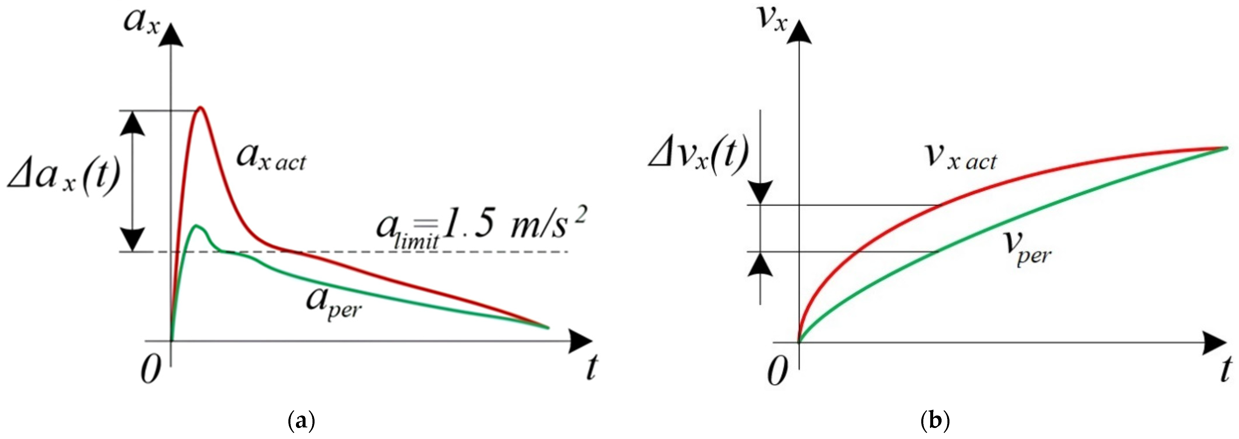
• $∆a_x\left(t_0\right)$—maximum acceleration difference, m/s²;
• ${\dot{a}}_x\left(t_0\right)$—derivative of acceleration (jerk) of the vehicle during acceleration reduction, which should not exceed 2 m/s³ [4].

Evidently, it is impossible to limit acceleration immediately. The process of achieving an acceleration of an acceptable value is aperiodic in nature. A graph explaining the meaning of the inertial constant and the aperiodic process of stabilization of acceleration is shown in Figure 3.

It is known that the transition process is 95% completed at time $3t_j$ During this period of time, the controller must complete the control process. Then, the integration time constant is $T_I.$ The PI controller can take the time of the steady-state transient of the inertial link and coefficient $K_I.$ The PI controller can be written using the following formula:

$$T_I=3t_j;K_I={\displaystyle \frac{1}{3t_j}}={\displaystyle \frac{1}{T_I}}.$$

(22)

In addition to the coefficient of the integral component $K_I$, it is also necessary to determine the value of the proportional coefficient $K_P$. It is known that the proportional coefficient is selected empirically based on the transition process requirements. However, to simplify the process of selecting coefficient $K_P$, it is necessary to narrow down the range of possible numeric values. The order of the numbers of the proportional coefficient can be determined as follows. The time constant $t_j$ also determines for what period of time the value of the multiplier should be lowered to a value at which the acceleration is reduced and maintained to the required value on a horizontal surface. Then, the order of the numbers of the calculated proportional coefficient can be determined by the following formula:

$$K_{Pcalc}={\displaystyle \frac{h_{acc}\left(t_0\right)-h_{acc}\left(t_{\infty }\right)}{t_j}},$$

(23)

where

• $h_{acc}\left(t_0\right)$—the magnitude of the control action at the initial moment of time;
• $h_{acc}\left(t_{\infty }\right)$—the magnitude of the control action when acceleration is limited.

From the nature of the transition process (Figure 3) and Formula (10), it is obvious that selecting a coefficient $K_P$ that is less than $K_{Pcalc}$ is impractical, since this would lead to an insufficiently intense decrease in the torque (Figure 4a,b), which will lead to a prolonged excess of acceleration compared to the permissible value. That is, the calibration process (if necessary) should start from the value $K_{Pcalc}$ and increase cyclically by 5% of the calculated amount. However, if the coefficient $K_P$ significantly exceeds $K_{Pcalc}$, then the intensity of torque reduction will be excessive; this would lead to a “loss” of acceleration (Figure 4c,d). The process of increasing the coefficient during calibration should end when the acceleration of the vehicle becomes stable a few seconds after the start of operation of the regulator.

4. Mathematical Modeling of Electric Bus Motion

Before implementing the developed system, one should study the operability and efficiency of the proposed laws and algorithms. The mathematical model of spatial motion was developed and verified based on the methods and principles outlined in several works [13,14,15,16,17,18,19]. It contains models of vehicle body dynamics, wheel rolling on the support base, elements of the underride system, and an uneven support base.

The motion of an electric bus with a curb weight of 12 tons was modeled, since, at this weight, the most intensive acceleration was possible. The characteristics of the KAMAZ 6282 electric bus [20] were used as a virtual prototype. The motion along a horizontal rectilinear trajectory was considered. Instantaneous pressing of the accelerator pedal to 100% was carried out at 5 s. The threshold acceleration was set to $a_{limit}$ = 1.5 m/s².

Motion modeling was performed for two vehicles: “Electric Bus 1” and “Electric Bus 2”. Electric Bus 1 had no longitudinal acceleration limitation, while Electric Bus 2 used the acceleration limitation algorithm. Figure 5 and Figure 6 show the longitudinal acceleration and linear velocity plots for both electric buses.

Figure 5 shows that the Electric Bus 1 reached an acceleration of 2.5 m/s². At the same time, the acceleration exceeded the threshold value for 6.5 s. In Electric Bus 2, with the acceleration limitation system engaged, the acceleration reached 2.5 m/s² briefly and then, suppressed by the controller, decreased to 1.5 m/s² in 2.5 s. The graphs in Figure 4 show that, with the regulator engaged, Electric Bus 2 gained speed less intensely than Electric Bus 1.

The cumulative velocity $S_{cv}$ was used as the efficiency criterion. The cumulative velocity is the area in the figure bound by the threshold acceleration from below and the longitudinal acceleration from above (Figure 7). The formula for calculating the cumulative velocity is as follows:

$$S_{cv}=\underset{t_1}{\overset{t_2}{\int }}∆a_x\left(t\right)dt,$$

(24)

where

• $t_1$—initial moment of time of acceleration exceedance, s;
• $t_2$—final moment of time of acceleration exceedance, s.

Table 1. Cumulative velocities during the acceleration of electric buses.

	Electric Bus 1	Electric Bus 2	Relative Efficiency
Cumulative Velocity	$S_{cv}=4.05\mathrm{m}/\mathrm{s}$	$S_{cv}=0.92\mathrm{m}/\mathrm{s}$	$+77.28\%$

records the results of the calculations of the cumulative velocities. Figure 8 shows the graphs of the requested torques.

This shows that the requested torque of Electric Bus 1 reached the maximum value of 780 N∙m and was held at this level for 3 s, while the requested torque of Electric Bus 2 reached a maximum value of 730 N∙m and then decreased to 500 N∙m under the action of the PI controller.

5. Field Tests of the Electric Bus—Justification of Operability and Efficiency of the Developed System

After virtual tests, the developed algorithm was tested on a real object. The KAMAZ 6282 electric bus was used as the test object [20] (Figure 9). The technical specifications are given in

Table 2. Technical specifications of the KAMAZ 6282 electric bus at testing.

Max speed	72 km/h
Vehicle mass	12,000 kg
Type of motor	Synchronous
Max peak torque	390 × 2 N∙m
Peak power	125 × 2 kW
Tires	275/70 R22.5

.

The tests were carried out at the KAMAZ test site. A standard inertial sensor supplied with the braking system was used as the device for measuring longitudinal acceleration, the signals of which were transmitted via the CAN bus [3]. A specialized software package for reading CAN messages was used for collecting data from the on-board CAN bus.

During the tests, straight-line acceleration was first performed with the longitudinal acceleration limitation system deactivated. The driver instantly pressed the accelerator pedal to 100%.

Figure 10 shows that the electric bus without software acceleration limitation developed an acceleration of up to 2.3 m/s². The acceleration exceeded the threshold value for 3.7 s.

A similar run was then conducted with the longitudinal acceleration limitation system activated. The driver also pressed the accelerator pedal to 100% instantaneously.

Figure 11 shows that the electric bus developed an acceleration up to 2 m/s², and then the acceleration began to decrease intensively, suppressed by the controller. The acceleration exceeded the relative threshold (1.5 m/s²) for 2.3 s.

Table 3. Cumulative velocities obtained during the test runs.

View of Electric Bus Arrival	With Unlimited Acceleration	With Limited Acceleration	Relative Efficiency
Cumulative Velocity	$S_{cv}=1.74\mathrm{m}/\mathrm{s}$	$S_{cv}=0.84\mathrm{m}/\mathrm{s}$	$+51.72\%$

records the cumulative velocity values obtained during the test runs.

The results show that the cumulative speed of the electric bus with an activated acceleration limitation system was lower. After the test runs, it could be concluded that the lower the cumulative speed, the higher the comfort and safety.

6. Conclusions

The results of this study allowed us to draw the following conclusions:

• The authors developed a system for limiting longitudinal acceleration, alongside the laws and algorithms of the control system, including the design of a regulator capable of limiting the longitudinal acceleration of a vehicle;
• The concept of total speed was introduced as a criterion for the effectiveness of the system;
• Mathematical modeling methods were used to prove the effectiveness of the algorithm at the stage of creating a system based on a virtual prototype of an electric bus. The relative efficiency of the system was 77.28%;
• The developed system was tested on the KAMAZ 6282 electric bus at the KAMAZ test site. During full-scale tests, the longitudinal acceleration did not exceed 2 m/s² and then lowered to 1.5 m/s², which is comfortable. At the same time, the relative efficiency was 51.72%;
• The practical significance of the algorithm for limiting longitudinal acceleration was proven during subsequent introduction into mass production.

References

1. Ovsyannikov, E.M. Traction Electrical Systems of Motor Transport Vehicles: Textbook; Forum, M., Ed.; INFRA-M: Moscow, Russia, 2019; p. 303. ISBN 978-5-00091-527-1. [Google Scholar]
2. Bokare, P.S.; Maurya, A.K. Acceleration-Deceleration Behavior of Various Vehicle Types. Transp. Res. Procedia 2017, 25, 4733–4749. [Google Scholar] [CrossRef]
3. Damian, F.; Grabski, P.; Jurecki, R.S.; Szumska, E.M. Experimental Study on Longitudinal Acceleration of Urban Buses and Coaches in Different Road Maneuvers. Sensors 2023, 23, 3125. [Google Scholar] [CrossRef] [PubMed]
4. Biryukov, V.V. Traction Electric Drive: Textbook for Universities, 2nd ed.; Yurait Publishing House: Moscow, Russia, 2021; p. 315. ISBN 978-5-534-04376-1. [Google Scholar]
5. Khajepour, A.; Fallah, S.; Goodarzi, A. Electric and Hybrid Vehicles. Technologies, Modeling and Control: A Mechatronic Approach; John Wiley & Sons Ltd.: Chichester, UK, 2014; 432p, ISBN 978-1-118-34151-3. [Google Scholar]
6. Barabino, B.; Eboli, L.; Mazzulla, G.; Mozzoni, S.; Murru, R.; Pungillo, G. An innovative methodology to define the bus comfort level. Transp. Res. Procedia 2019, 41, 461–470. [Google Scholar] [CrossRef]
7. Krasna, S.; Keller, A.; Linder, A.; Silvano, A.P.; Xu, J.C.; Tompson, R.; Klug, C. Human Response to Longitudinal Perturbations of Standing Passengers on Public Transport During Regular Operation. Front. Bioeng. Biotechnol. 2021, 9, 680883. [Google Scholar] [CrossRef] [PubMed]
8. Lobusov, E.S.; Zhileikin, M.M. Algorithm of definition of actual speed for maintenance of work of the automated control system of movement of a wheeled machine. Izvestiya Vuzov. Mashinostroenie 2017, 7, 34–40. [Google Scholar] [CrossRef]
9. Tarasik, V.P. Theory of Car Movement, 2nd ed.; BHV-Peterburg: Berlin, Germany, 2022; p. 576. ISBN 978-5-9775-6817-3. [Google Scholar]
10. Larin, V.V. Theory of Motion of All-Wheel Drive Wheeled Machines: A Textbook for Universities; Bauman Moscow State Technical University: Moscow, Russia, 2010; 391p, ISBN 978-5-7038-3389-6. [Google Scholar]
11. Ivanov, V.A.; Faldin, N.V. Theory of Optimal Automatic Control Systems; Nauka. Main Editorial Office of Physical and Mathematical Literature: Moscow, Russia, 1981; 336p. [Google Scholar]
12. Denisenko, V.V. Computer Control of Technological Process, Experiment, Equipment; Hot Line-Telecom: Moscow, Russia, 2011; 608p, ISBN 978-5-9912-006-8. [Google Scholar]
13. Büschgens, G.S.; Studnev, R.V. Dynamics of Aircraft. Spatial Motion; Mashinostroenie: Moscow, Russia, 1983; 320p. [Google Scholar]
14. Dik, A.B. Calculation of Stationary and Non-Stationary Characteristics of a Braking Wheel in a Drift Motion. Ph.D. Thesis, Siberian State Automobile and Highway University (SibADI), Omsk, Russia, 1988. [Google Scholar]
15. Rozhdestvenskiy, Y.L.; Mashkov, K.Y. About the reaction formation when an elastic wheel rolls on a non-deformable support base. Proc. MVTU 1982, 390, 56–64. [Google Scholar]
16. Shadrin, S.S. Methodology of Calculation Estimation of Controllability and Stability of a Car. Ph.D. Thesis, Moscow Automobile and Road Construction State Technical University, Moscow, Russia, 2005. [Google Scholar]
17. Rajamani, R. Vehicle Dynamics and Control, 2nd ed.; Springer: Berlin/Heidelberg, Germany, 2012; 496p, ISBN 978-1-46141433-9. [Google Scholar]
18. Jazar, R.N. Vehicle Dynamics. Theory and Application; Springer: Berlin/Heidelberg, Germany, 2008; 1022p, ISBN 987-0-387-74243-4. [Google Scholar]
19. Kienke, U.; Nielsen, L. Automotive Control Systems. For Engine, Driveline, and Vehicle, 2nd ed.; Springer: Berlin/Heidelberg, Germany, 2005; 512p, ISBN 978-3-540-26484-2. [Google Scholar]
20. Kamaz, L.L.C. Characteristics of Electric Bus KAMAZ 6282, Naberezhnye Chelny. Available online: https://kamaz.ru/production/buses/pdf/Электробус%20KAMAZ-6282.pdf (accessed on 9 September 2022).
Figure 1. Graphs explaining the regulator design principle: (a) acceleration and (b) velocity graphs.
Vehicles 07 00007 g001
Figure 2. Structural diagram of the requested torque generation.
Vehicles 07 00007 g002
Figure 3. Graphs of reaching the maximum speed of movement: (a) speed graph and (b) the schedule of the control action.
Vehicles 07 00007 g003
Figure 4. Graphs of reaching the maximum speed at different values of the proportional coefficient K P : (a) graph of the speed at K P < K P   c a l c ; (b) schedule of the control action at K P < K P   c a l c ; (c) graph of the speed at K P > K P   c a l c ; and (d) schedule of the control action at K P > K P   c a l c .
Vehicles 07 00007 g004
Figure 5. Plots of longitudinal acceleration a x : red graph, Electric Bus 1; green graph, Electric Bus 2; and dashed line, threshold value equal to a l i m = 1.5   m / s 2 .
Vehicles 07 00007 g005
Figure 6. Graphs of linear velocity v x : red graph, linear velocity of Electric Bus 1; and green graph, Electric Bus 2.
Vehicles 07 00007 g006
Figure 7. Graph explaining the concept of cumulative velocity.
Vehicles 07 00007 g007
Figure 8. Graphs of the requested torques: red graph, Electric Bus 1; and green graph, Electric Bus 2.
Vehicles 07 00007 g008
Figure 9. KAMAZ 6282 electric bus at testing.
Vehicles 07 00007 g009
Figure 10. Longitudinal acceleration graph for the electric bus without acceleration limitation.
Vehicles 07 00007 g010
Figure 11. Longitudinal acceleration graph for the electric bus with acceleration limitation.
Vehicles 07 00007 g011