

Investigation and Phenomenological Modeling of Degraded Twin-Tube Shock Absorbers for Oil and Gas Loss


Abstract
1. Introduction
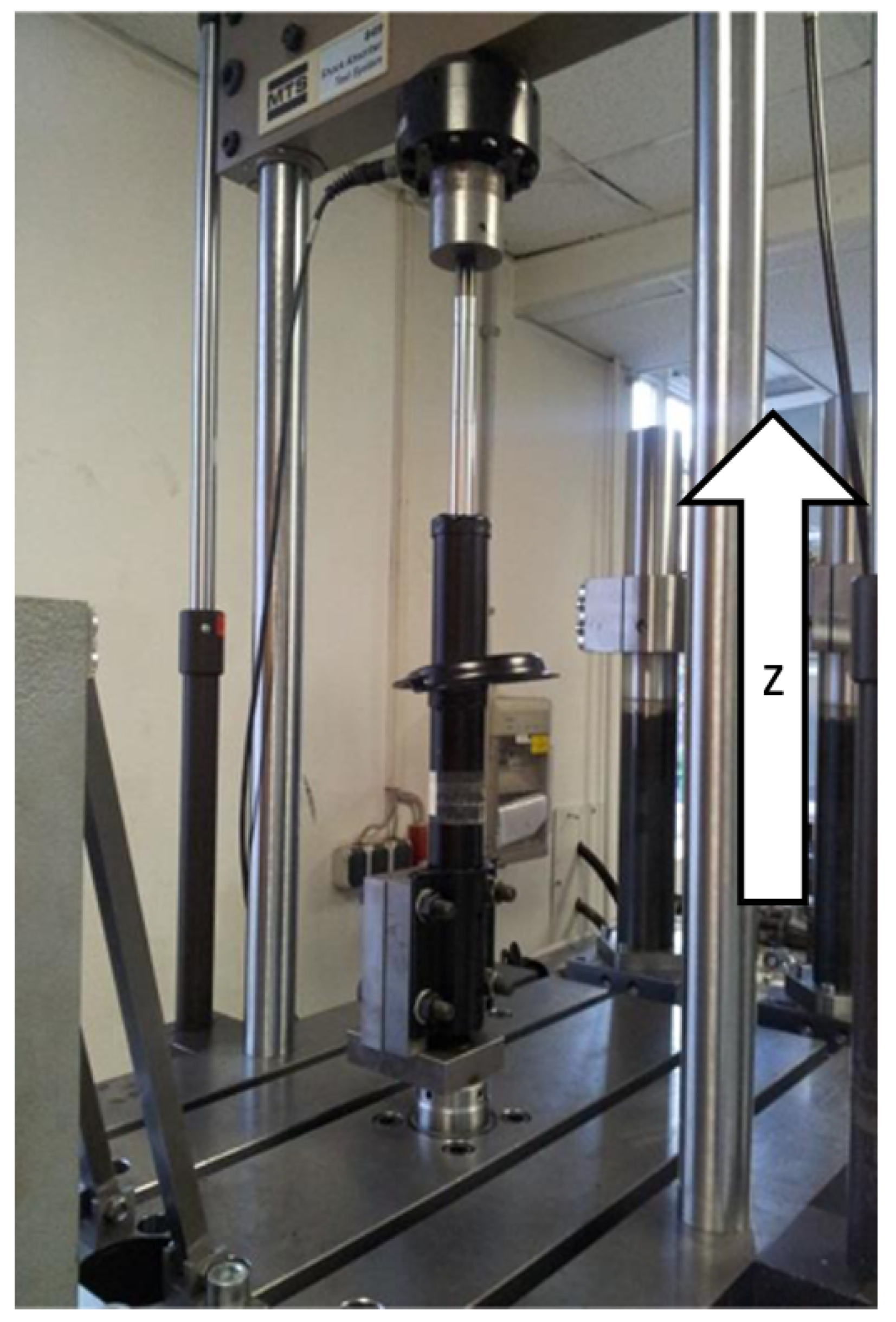
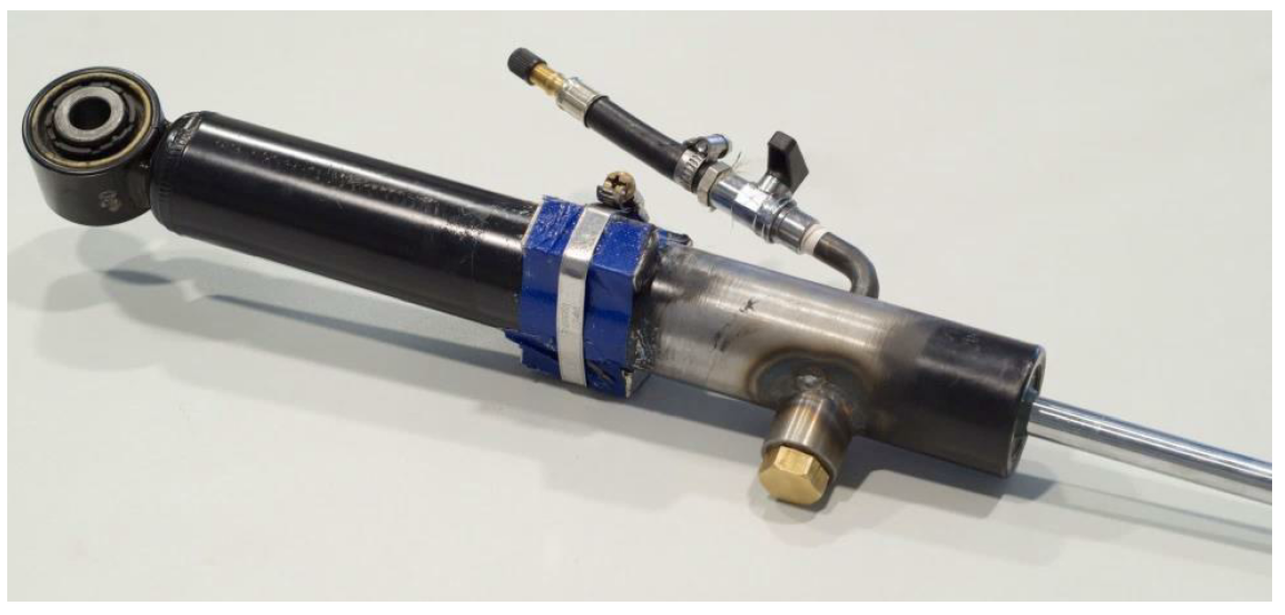
2. Materials and Methods
3. Results
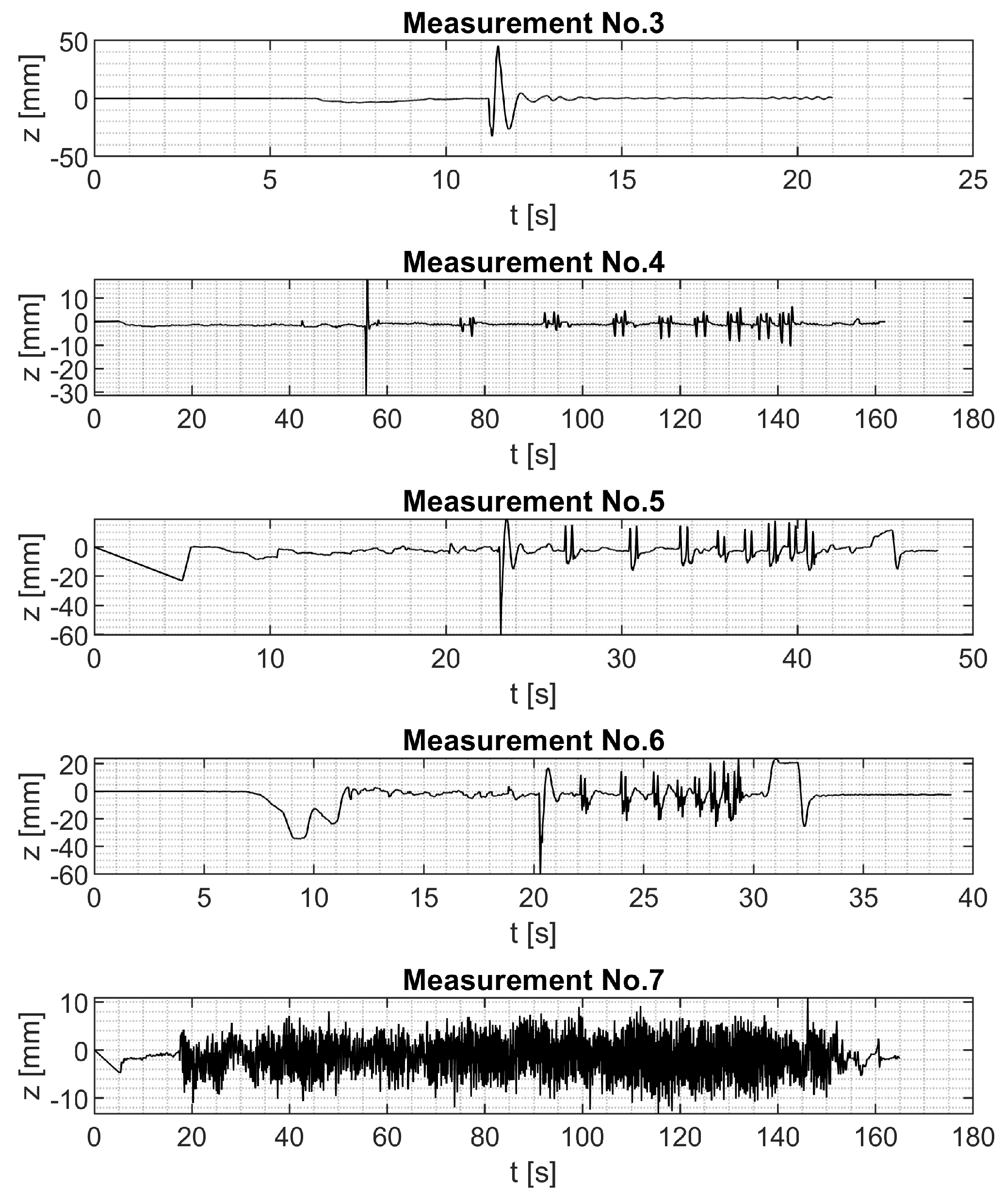
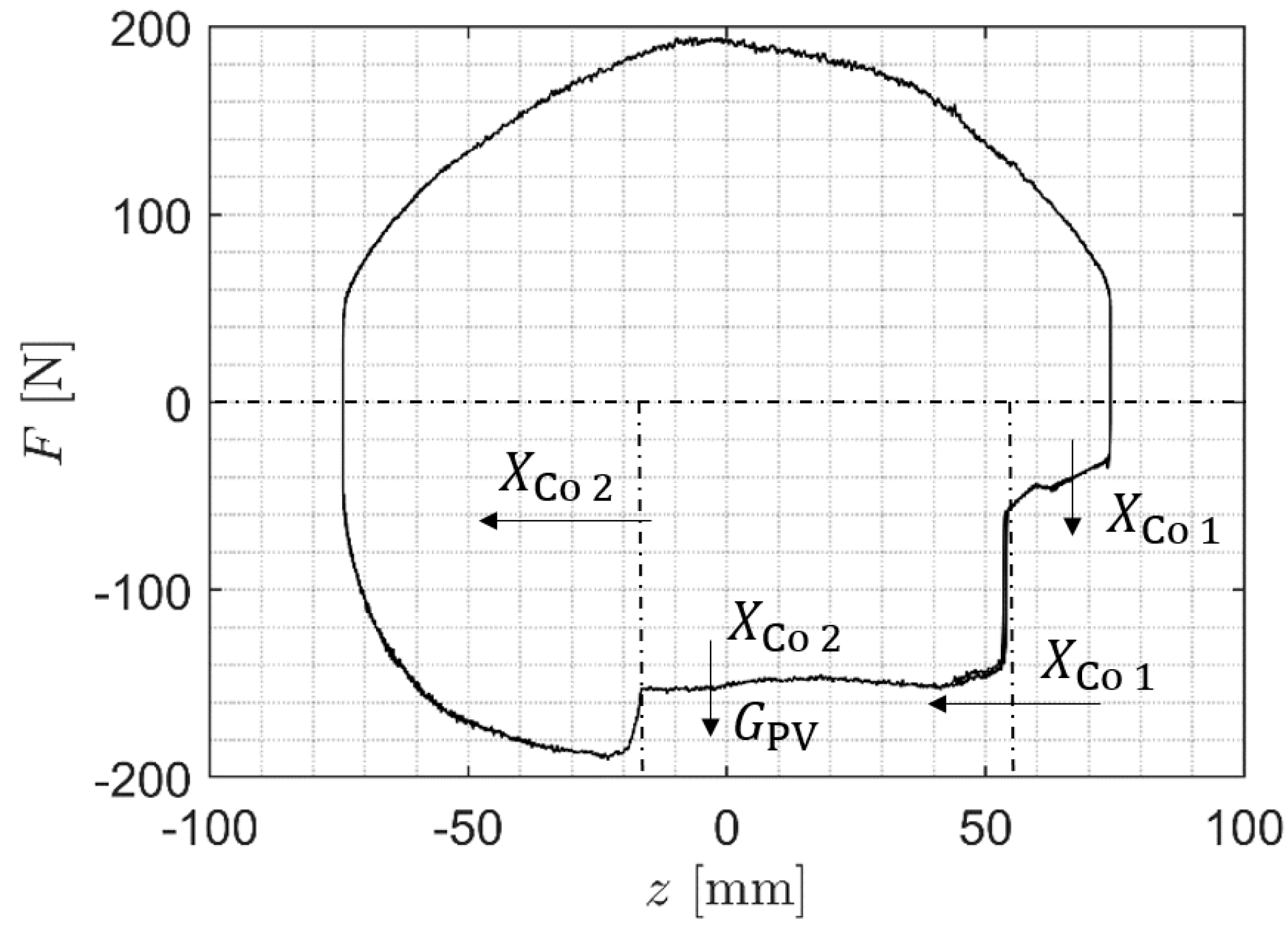
3.1. Data Analysis
3.2. Shock Absorber Model
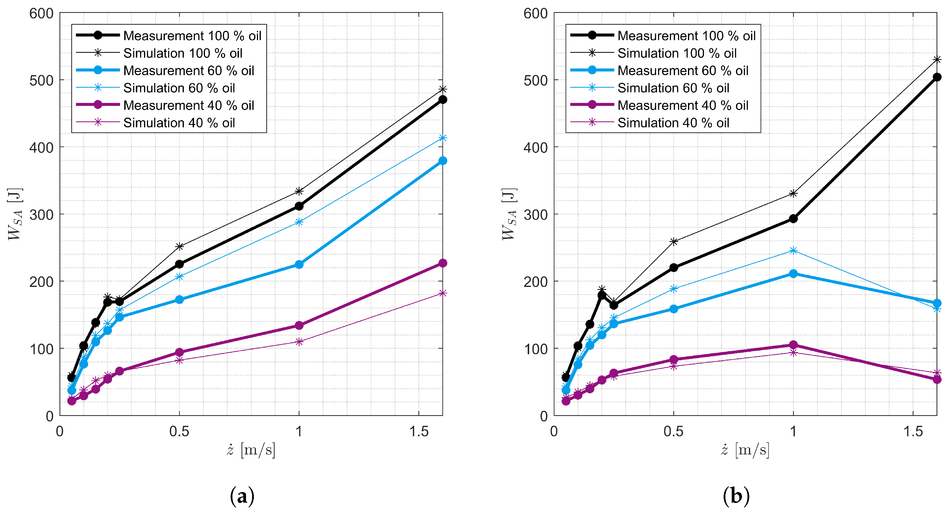
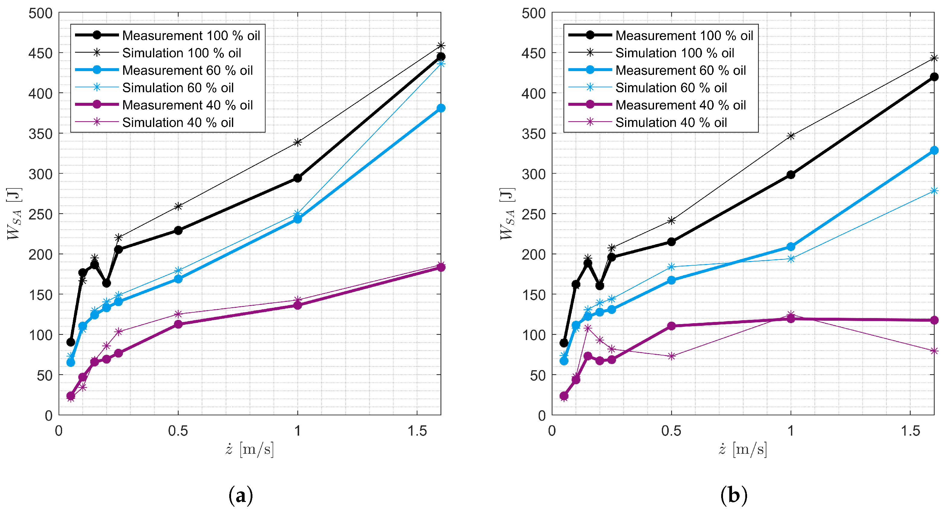
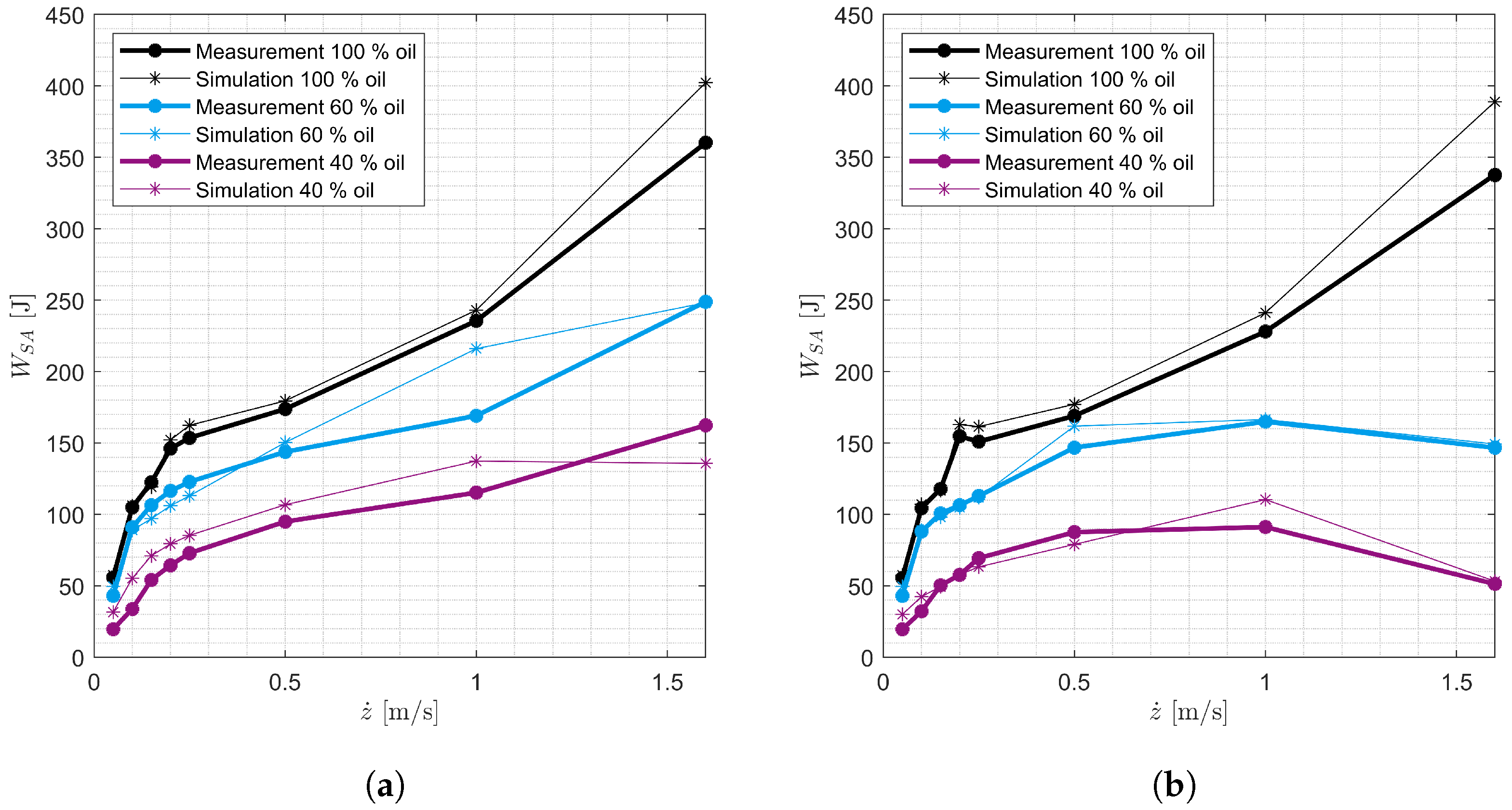
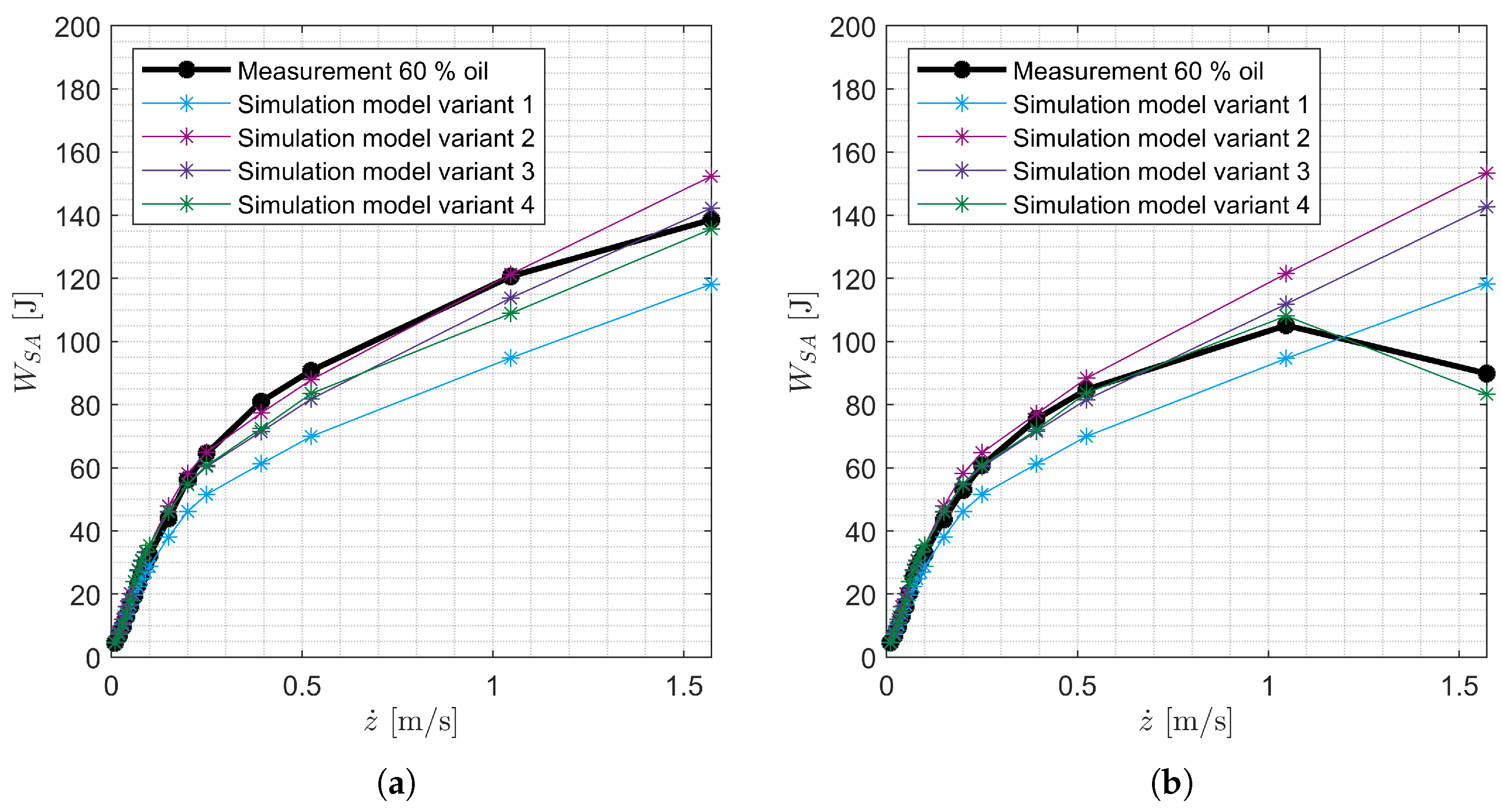
3.3. Validation
3.4. Simulation Study
4. Discussion
5. Conclusions
Author Contributions
Funding
Data Availability Statement
Acknowledgments
Conflicts of Interest
Abbreviations
| ABS | Anti-lock braking system |
| SA | Shock absorber |
| F-v | Force–velocity |
| F-s | Force–displacement |
| PV | Piston valve |
| BV | Bottom valve |
| PR | Piston rod |
| OS | Shock absorber seal |
| IT | Inner tube wall of the shock absorber |
| PSO | Particle swarm optimization |
References
- Wegener, D.B. Prüfverfahren für Schwingungsdämpfer im Fahrzeug. Ph.D. Thesis, RWTH Aachen University, Aachen, Germany, 2020. [Google Scholar] [CrossRef]
- Rompe, K.; Grunow, D. Stoßdämpfer und Fahrsicherheit. Verk. Fahrz. 1996, 34, 2–6. [Google Scholar]
- Vaculín, O.; Svoboda, J.; Valášek, M.; Steinbauer, P. Influence of deteriorated suspension components on ABS braking. Veh. Syst. Dyn. 2008, 46, 969–979. [Google Scholar] [CrossRef]
- Zwosta, T.; Kubenz, J.; Prokop, G. Experimental Analysis of the Influence of Damper Degradation by Loss of Oil on the Straight Braking Performance of Passenger Cars with ABS; SAE: Warrendale, PA, USA, 2024. [Google Scholar] [CrossRef]
- Rompe, K. TÜV Kraftfahrt GmbH Köln: Warum muss die Wirksamkeit der Stoßdämpfer regelmäßig überprüft werden? TÜ 1998, 39, 13–17. [Google Scholar]
- Laermann, F.J. SeifenfüHrungsverhalten von Kraftfahrzeugen bei Schnellen Radlaständerungen; VDI Fortschrittsberichte: Düsseldorf, Germany, 1986; Volume 12. [Google Scholar]
- Parczewski, K. Exploration of the shock-absorber damage influence on the steerability and stability of the car motion. J. KONES 2011, 18, 331–338. [Google Scholar]
- Schramm, T.; Prokop, G. Simulative Study of the Influence of Degraded Twin-Tube Shock Absorbers on the Lateral Forces of Vehicle Axles. In Proceedings of the FISITA 2023 World Congress, Barcelona, Spain, 12–15 September 2023. [Google Scholar] [CrossRef]
- Zwosta, T. Experimental Analysis of the Behavior of Automotive Twin-Tube Dampers Degraded by Loss of Oil and Pressure; SAE: Warrendale, PA, USA, 2023. [Google Scholar] [CrossRef]
- Czop, P.; Wszołek, G.; Hetmańczyk, M.P. The Effects of the Aeration Phenomenon on the Performance of Hydraulic Shock Absorbers. In Modelling in Engineering 2020: Applied Mechanics; Mężyk, A., Kciuk, S., Szewczyk, R., Duda, S., Eds.; Advances in Intelligent Systems and Computing; Springer International Publishing: Cham, Switzerland, 2021; Volume 1336, pp. 11–30. [Google Scholar]
- Czop, P.; Gniłka, J. A Quick-and-Dirty Method for Assessing the Risk of Negative Aeration Effects of Shock Absorbers Equipped with Shim Sliding Base Valves. Comput. Assist. Methods Eng. Sci. 2022, 29, 229–260. [Google Scholar] [CrossRef]
- Hu, S.; Yang, M.; Meng, D.; Hu, R. Damping performance of the degraded fluid viscous damper due to oil leakage. Structures 2023, 48, 1609–1619. [Google Scholar] [CrossRef]
- Gao, H.; Sun, J.; E, S.; Chi, M. Cavitation induced hydraulic yaw damper failure and its effect on railway vehicle dynamic stability. Eng. Fail. Anal. 2024, 161, 108318. [Google Scholar] [CrossRef]
- Gao, H.; Chi, M.; Dai, L.; Yang, J.; Zhou, X. Mathematical Modelling and Computational Simulation of the Hydraulic Damper during the Orifice-Working Stage for Railway Vehicles. Math. Probl. Eng. 2020, 2020, 1–23. [Google Scholar] [CrossRef]
- Gao, J.; Wu, F.; Li, Z. Study on the Effect of Stiffness Matching of Anti-Roll Bar in Front and Rear of Vehicle on the Handling Stability. Int. J. Automot. Technol. 2021, 22, 185–199. [Google Scholar] [CrossRef]
- Dai, L.; Chi, M.; Guo, Z.; Gao, H.; Wu, X.; Sun, J.; Liang, S. A physical model-neural network coupled modelling methodology of the hydraulic damper for railway vehicles. Veh. Syst. Dyn. 2023, 61, 616–637. [Google Scholar] [CrossRef]
- Hryciów, Z.; Rybak, P.; Gieleta, R. The influence of temperature on the damping characteristic of hydraulic shock absorbers. Eksploat. I Niezawodn.-Maint. Reliab. 2021, 23, 346–351. [Google Scholar] [CrossRef]
- Hryciów, Z. An Investigation of the Influence of Temperature and Technical Condition on the Hydraulic Shock Absorber Characteristics. Appl. Sci. 2022, 12, 12765. [Google Scholar] [CrossRef]
- Georgiev, Z. Method for determining the technical condition of telescopic shock absorbers. In Proceedings of the 14th International Scientific Conference on Aeronautics, Automotive, and Railway Engineering and Technologies, Sozopol, Bulgaria, 10–13 September 2022; AIP Conference Proceedings. AIP Publishing: Melville, NY, USA, 2024; p. 030003. [Google Scholar] [CrossRef]
- Gajek, A. Directions for the development of periodic technical inspection for motor vehicles safety systems. Arch. Automot. Eng.-Arch. Motoryz. 2018, 80, 37–51. [Google Scholar] [CrossRef]
- Duym, S.W. Simulation Tools, Modelling and Identification, for an Automotive Shock Absorber in the Context of Vehicle Dynamics. Veh. Syst. Dyn. 2000, 33, 261–285. [Google Scholar] [CrossRef]
- Pfeffer, P.E.; Benz, D. A new method for damper characterization and real time capable modeling for ride comfort. In Proceedings of the FISITA World Automotive Congresss 2018, Chennai, India, 2–5 October 2018. [Google Scholar]
- Deubel, C.; Schubert, B.; Prokop, G. Velocity and Load Dependent Shock Absorber Friction under Stationary Conditions. Tribol. Int. 2023, 193, 109424. [Google Scholar] [CrossRef]
- Stribeck, R. Die wesentlichen Eigenschaften der Gleit- und Rollenlager. Z. Vereines Dtsch. Ing. 1902, 46, 1341–1348. [Google Scholar]
- Küper, K. Physikalische Modellbildung von Schwingungsdämpfern zur Analyse des dynamischen Verhaltens und dessen Wirkung auf Unstetigkeiten im Kraftaufbau. Ph.D. Thesis, Ruhr University Bochum, Bochum, Germany, 2011. [Google Scholar]
- Jablonská, J.; Kozubková, M.; Marcalík, P. Experimental circuit for the generation of cavitation in oil flow. EPJ Web Conf. 2022, 269, 01022. [Google Scholar] [CrossRef]
- Chen, Q.; Wu, M.; Kang, S.; Liu, Y.; Wei, J. Study on cavitation phenomenon of twin-tube hydraulic shock absorber based on CFD. Eng. Appl. Comput. Fluid Mech. 2019, 13, 1049–1062. [Google Scholar] [CrossRef]
- Totten, G.E.; Sun, Y.H.; Bishop, R.J., Jr.; Lin, X. Hydraulic System Cavitation: A Review. J. Commer. Veh. 1998, 107, 368–380. [Google Scholar] [CrossRef]


| Shock Absorber No. | Vehicle | Axle |
|---|---|---|
| 1 | Volkswagen Golf VI | Front |
| 2 | Volkswagen Golf VI | Rear |
| 3 | Volkswagen Passat B6 | Front |
| 4 | Volkswagen Passat B6 | Rear |
| 5 | Volkswagen Caddy III | Front |
| 6 | Volkswagen Caddy III | Rear |
| 7 | Volkswagen Passat B8 | Front |
| 8 | Volkswagen Passat B8 | Rear |
| Shock Absorber | 1 | 2 | ||||||
| Condition [%] | 100 | 60 | 40 | 0 | 100 | 60 | 40 | 0 |
| Real oil volume [mL] | 321 | 161 | 112 | 0 | 264 | 166 | 106 | 0 |
| Real oil proportion [%] | 100 | 50 | 35 | 0 | 100 | 63 | 40 | 0 |
| Shock Absorber | 3 | 4 | ||||||
| Condition [%] | 100 | 60 | 40 | 0 | 100 | 60 | 40 | 0 |
| Real oil volume [mL] | 371 | 226 | 148 | 0 | 239 | 160 | 96 | 0 |
| Real oil proportion [%] | 100 | 61 | 40 | 0 | 100 | 67 | 40 | 0 |
| Shock Absorber | 5 | 6 | ||||||
| Condition [%] | 100 | 60 | 40 | 0 | 100 | 60 | 40 | 0 |
| Real oil volume [mL] | 332 | 239 | 133 | 0 | 153 | 95 | 61 | 0 |
| Real oil proportion [%] | 100 | 72 | 40 | 0 | 100 | 62 | 40 | 0 |
| Shock Absorber | 7 | 8 | ||||||
| Condition [%] | 100 | 60 | 40 | 0 | 100 | 60 | 40 | 0 |
| Real oil volume [mL] | 354 | 194 | 114 | 0 | 273 | 153 | 83 | 0 |
| Real oil proportion [%] | 100 | 55 | 32 | 0 | 100 | 56 | 30 | 0 |
| No. | Measurement |
|---|---|
| 1 | Quasi-static measurements |
| 2 | Harmonic measurements |
| 3 | Speed bump crossing 8 km/h |
| 4 | Cleat crossings 4 km/h |
| 5 | Cleat crossings 20 km/h |
| 6 | Cleat crossings 40 km/h |
| 7 | Uneven road washboard 4 km/h |
| 8 | Uneven road braking maneuver from 30 km/h |
| 9 | Uneven road braking maneuver from 50 km/h |
| 10 | Uneven road drive 4 km/h |
| 11 | Uneven road drive 30 km/h |
| 12 | Uneven road drive 50 km/h |
| Formula Symbol | Description |
|---|---|
| Simulation timestep | |
| z | Piston rod displacement; stroke |
| Piston rod velocity | |
| Area of the piston valve to the rebound chamber | |
| Area of the piston valve to the compression chamber | |
| Volume of the rebound chamber | |
| Volume of the compression chamber | |
| Volume of the reserve chamber | |
| Pressure in rebound chamber | |
| Pressure in compression chamber | |
| Total shock absorber force | |
| Shock absorber gas force | |
| Shock absorber friction force | |
| Shock absorber fluid friction force | |
| Degradation factor | |
| Gas spring stiffness | |
| Slope of the hysteresis loop | |
| saturated quasi-static friction force | |
| Exponent of the hysteresis friction gradient | |
| F-v-characteristic | |
| Volume flow rate | |
| Relative oil volume flow | |
| Relative oil volume flow change | |
| Cavitation treshold velocity | |
| Cavitation factor | |
| Total measured shock absorber force | |
| Total simulated shock absorber force | |
| Total measured shock absorber work | |
| Total simulated shock absorber work |
| Dimensions [mm] | SA 1 | SA 2 | SA 3 | SA 4 | SA 5 | SA 6 | SA 7 | SA 8 |
|---|---|---|---|---|---|---|---|---|
| 45.50 | 41.20 | 50.20 | 41.20 | 46.60 | 38.00 | 50.00 | 41.40 | |
| 22.00 | 13.00 | 25.00 | 13.00 | 25.00 | 14.00 | 25.00 | 13.00 | |
| 32.00 | 29.90 | 35.90 | 30.00 | 36.00 | 27.00 | 35.80 | 29.80 | |
| 34.80 | 32.00 | 38.65 | 32.00 | 38.60 | 29.00 | 38.60 | 32.10 | |
| 326.00 | 277.90 | 326.00 | 277.90 | 328.00 | 225.70 | 326.00 | 331.00 |
| Parameter | Definition |
|---|---|
| Oil proportion that flows through the PV simultaneously with gas during rebound | |
| Leakage factor; proportion of oil that flows through the PV without generating a damping force | |
| Proportion of the oil that flows through the PV and not through the BV during the compression stroke | |
| Oil proportion that flows through the PV simultaneously with gas during compression stroke | |
| Oil flow proportion from through the PV in relation to the total oil outflow from in the compression stage when is completely filled with oil |
| Parameter | Definition |
|---|---|
| Proportion of the gas volume flow through the BV, which is converted into foam during the rebound stroke | |
| Oil proportion of the foam that is generated in the BV during the rebound stroke | |
| Proportion of the gas volume flow through the PV, which is converted into foam during the compression stroke | |
| Oil proportion of the foam that is formed in the PV during the compression stroke | |
| B | Properties of the foam more like oil (B = 1) or gas (B = 0) |
| E | Relationship between oil proportion of the foam and damping force |
| Parameter | Definition |
|---|---|
| Cavitation model treshold velocity | |
| Oil proportion which is transformed into gas during compression | |
| Oil proportion which is transformed into gas during rebound |
| Parameter | SA 1 | SA 2 | SA 3 | SA 4 | SA 5 | SA 6 | SA 7 | SA 8 |
|---|---|---|---|---|---|---|---|---|
| 0.20 | 0.16 | 0.13 | 0.13 | 0.30 | 0.08 | 0.00 | 0.01 | |
| 0.59 | 0.90 | 0.01 | 0.10 | 0.90 | 0.74 | 0.00 | 0.06 | |
| 0.01 | 0.00 | 0.27 | 0.02 | 0.00 | 0.00 | 0.49 | 0.01 | |
| 0.00 | 0.14 | 0.01 | 0.04 | 0.10 | 0.07 | 0.00 | 0.15 | |
| 0.59 | 0.24 | 0.13 | 0.37 | 0.43 | 0.29 | 0.16 | 0.94 | |
| 0.07 | 1.00 | 1.00 | 0.29 | 0.10 | 0.17 | 0.00 | 0.94 | |
| 0.20 | 0.43 | 0.19 | 0.00 | 0.27 | 0.02 | 0.44 | 1.00 | |
| 1.00 | 0.00 | 0.61 | 0.93 | 0.26 | 0.28 | 0.02 | 0.72 | |
| 0.00 | 0.44 | 1.00 | 0.44 | 0.17 | 0.42 | 0.00 | 0.15 | |
| B | 0.90 | 0.81 | 0.23 | 0.73 | 0.94 | 1.00 | 0.34 | 0.38 |
| E | 48.24 | 26.01 | 13.60 | 50.00 | 92.38 | 12.58 | 0.41 | 8.68 |
| 1.00 | 0.90 | 1.05 | 0.00 | 0.95 | 0.00 | 0.70 | 0.90 | |
| 0.04 | 0.03 | 0.03 | 0.00 | 0.04 | 0.00 | 0.05 | 0.20 | |
| 0.04 | 0.02 | 0.03 | 0.00 | 0.04 | 0.00 | 0.05 | 0.20 |
Disclaimer/Publisher’s Note: The statements, opinions and data contained in all publications are solely those of the individual author(s) and contributor(s) and not of MDPI and/or the editor(s). MDPI and/or the editor(s) disclaim responsibility for any injury to people or property resulting from any ideas, methods, instructions or products referred to in the content. |
© 2025 by the authors. Licensee MDPI, Basel, Switzerland. This article is an open access article distributed under the terms and conditions of the Creative Commons Attribution (CC BY) license (https://creativecommons.org/licenses/by/4.0/).
Share and Cite
Schramm, T.; Zwosta, T.; Prokop, G. Investigation and Phenomenological Modeling of Degraded Twin-Tube Shock Absorbers for Oil and Gas Loss. Vehicles 2025, 7, 26. https://doi.org/10.3390/vehicles7010026
Schramm T, Zwosta T, Prokop G. Investigation and Phenomenological Modeling of Degraded Twin-Tube Shock Absorbers for Oil and Gas Loss. Vehicles. 2025; 7(1):26. https://doi.org/10.3390/vehicles7010026
Chicago/Turabian StyleSchramm, Tobias, Tobias Zwosta, and Günther Prokop. 2025. "Investigation and Phenomenological Modeling of Degraded Twin-Tube Shock Absorbers for Oil and Gas Loss" Vehicles 7, no. 1: 26. https://doi.org/10.3390/vehicles7010026
APA StyleSchramm, T., Zwosta, T., & Prokop, G. (2025). Investigation and Phenomenological Modeling of Degraded Twin-Tube Shock Absorbers for Oil and Gas Loss. Vehicles, 7(1), 26. https://doi.org/10.3390/vehicles7010026