Planning Integrated Unmanned Aerial Vehicle and Conventional Vehicle Delivery Operations under Restricted Airspace: A Mixed Nested Genetic Algorithm and Geographic Information System-Assisted Optimization Approach

Abstract

Using Unmanned Aerial Vehicles (UAVs), commonly referred to as “drones”, as a supplementary mode for last-mile deliveries has been a research focus for some years now. Motivation lies in the reduced dependency on Conventional Vehicles (CVs) and fossil fuels and in serving remote areas and underprivileged populations. We are building a flexible, modular framework for integrated CV-UAV parcel delivery operations planning that is responsive to infrastructure and demand and offers an open and practical tool for future adaptations. The entire model and solution methodology are practical tools for decision making and strategic planning, with novelties such as the variable Launch Site types for Launch and Recovery Operations (LAROs), the tailored Assignment and Routing Optimization nested GA, the consideration of airspace restrictions of any shape and size, the inclusion of GIS tools in the process, the modularity of the platform, and most importantly, the inclusion of all the above in a single, comprehensive, and holistic approach. Because of the need for safe UAV deployment sites and the high presence of restricted airspace zones in urban environments, the intended field of application is assumed to be the delivery of small packages in rural and under-connected areas, the execution of inter-city deliveries, and the expansion of a city’s original service range. A single CV is equipped onboard with UAVs, while special locations, such as Remote Depots (RDs) with UAVs and Virtual Hubs (VHs) for UAV deployment facilitation, are introduced. The framework considers the presence of Restricted Zones (RZs) for UAV flights. Part of the methodology is implemented in a GIS environment, taking advantage of modern tools for spatial analysis and optimal path planning. We have designed a tailored nested GA method for solving the occurring mode assignment and vehicle routing optimization problems and have implemented our workflow on a devised case study with benchmark characteristics. Our model responds well to unfavorable network types and demand locations, while the presence of RZs notably affects the expected solution and should be considered in the decision-making process.

1. Introduction

The transformation of the transport sector is a pivotal part of efforts towards a sustainable future, especially in cities. The EU has set ambitious targets for 2020–2030, aiming for a reduction of 40% of GHGs relative to 1990 levels and a share of 35% of zero- or low-emission new cars and vans by 2030 [1]. A 100% zero-emission fleet is envisioned in cities by 2050, and several countries are set to ban internal combustion engines in urban areas by 2032 [2]. In another context, rapid consumer behavioral changes have led to a significant increase in online shopping and at-home and at-work deliveries. Delivery services rely heavily on conventional vehicles running on fossil fuels, such as delivery trucks or vans, and this is especially true for last-mile deliveries, which could account for up to 20%–30% of a city’s CO₂ emissions [3].

The use of Unmanned Aerial Vehicles (UAVs), commonly referred to as drones, and other automated systems, like ground-level robots, is a novel concept that has already attracted the interest of tech and logistics companies; their involvement in transportation services is expected to have significant effects on various sectors, with their impact on the economy, the environment, employment, and infrastructure being a matter of ongoing research [4]. UAVs are commonly battery-powered, so if electricity can be generated from environmentally friendly sources (e.g., renewables), an overall reduction in emissions is expected [3]. Several UAV applications in transportation are identified in the literature, such as the automation of intralogistics, first/last-mile parcel delivery, supply of medical goods, or even transportation of air freight, when UAV specs allow [5]. Flytrex is using UAVs for deliveries in Iceland, and Eliport is developing small ground-level autonomous robots for the same purpose [3]. Blood samples are transported by Zipline in Rwanda, and medical goods are distributed by DHL’s “Parcelcopter” in Tanzania [5]. UAV-based transport, however, still faces challenges, ranging from societal acceptance concerning safety and privacy to regulatory hurdles and the mix with the rest of airborne traffic. More than 40% of respondents in various regions worldwide cite safety as their primary issue, while privacy (13–29%) and noise (9–21%) follow [6].

Despite active cases of tandem CV-UAV operations in parcel delivery, there is still some way to go in setting up reliable, scalable systems that can easily adapt to infrastructure and demand and be optimized for performance, assisting the strategic decision-making process. In the literature, the problem is commonly categorized in the wider Vehicle Routing Problem (VRP) family. It is essentially a concurrent mode assignment and vehicle routing problem where ground vehicles (usually trucks) are combined with drones to serve last-mile goods transport. The problem is more specifically named Vehicle Routing Problem with Drone (VRP-D), Truck and Drone Routing Problem (TDRP), or Two-Echelon Vehicle Routing Problem with Drone (2E VRP-D). The special actions concerning drone deployment are also commonly referred to as Launch and Recovery Operations (LAROs). Murray and Chu [7] introduced the “Flying Sidekick Traveling Salesman Problem” (FSTSP), where customers can be served either by a truck or a UAV (working in tandem), the latter being able to launch from the truck or the depot to customers and return to the same or a different location. Customer locations are also UAV deployment sites, and flight paths are straight, albeit restricted by the UAV’s range. Ferrandez et al. [8] used multiple UAVs and a truck, with the latter moving along a TSP route, and k-means clustering [9] was used to find optimal stop and launch locations. Moshref-Javadi et al. [10] assumed a single truck and multiple UAVs, considering routes only involving the depot and customer locations with identical take-off and landing points. Simulated annealing and tabu search were used to obtain efficient routing solutions, and there was also an application on a real-world network. Non-customer locations were included as potential UAV deployment sites by Salama and Srinivas (2022) [11], but all items lying on the truck’s route must be served by the truck, leading to a route-first, cluster-second solution approach, and using simulated annealing and variable neighborhood search for optimization. En-route deployment of UAVs was proposed by Marinelli et al. [12]; in this case, the truck can deploy UAVs by stopping at points along arcs and not only at nodes of the road network. Initially formed k-means clusters and then centers movement to determine the truck’s route via weight shifts were applied by Chand and Lee [13]. A route-first, cluster-second solution approach was also adopted by Agatz et al. [14], who employed local search and dynamic programming heuristics to solve a problem where launch sites only appeared at delivery locations and take-off and landing points for UAVs did not necessarily coincide.

With regards to more recent developments in research, González-Rodríguez et al. [15] considered the case of rechargeable drones that can meet with the truck for battery changes only at customer locations. They proposed using an iterated greedy heuristic based on the iterative process of destruction and reconstruction of solutions, assisted by a global optimization scheme through a simulated annealing (SA) algorithm. Jeong et al. [16] considered a model of different take-off and landing points, considering the effect of parcel weight on drone energy consumption and restricted flying areas of circular shape. They built a two-phase constructive and search heuristic algorithm to obtain optimal solutions. Salama and Srinivas [11] propose “flexible” sites for drone launch and recovery operations (LAROs), instead of only using customer locations for this purpose. They formulate a mixed integer linear programming model and solve it through an optimization-enabled two-phase search algorithm by hybridizing simulated annealing and variable neighborhood search. Their comparative experiments showed the improvements made by removing the “customer locations only” constraint for LARO. Zhou et al. [17] developed an exact algorithm for the solution of the two-echelon truck and drone problem. They consider multiple vehicles and drones and formulate the problem in a mixed-integer linear programming model that is also solvable with commercial software. Their own solution process comes through an exact branch-and-price algorithm, applied after an initial tabu search application. Momeni et al. [18] assumed different altitudes for package deliveries and calculated the drones’ energy consumption as affected by wind and weight. Deliveries are only made by drones, and a two-phase algorithm based on the nearest neighborhood and local search was used to solve the problem. Li et al. [19] moved from fixed locations to moving meeting points along the truck arcs (TDRP-SA), without the need for parking areas. An adaptive large neighborhood heuristic was used for obtaining optimal solutions, taking advantage of previously developed boundary models to locate moving launch and recovery locations (LRLs). Leon-Blanco et al. [20] developed an agent-based method to solve the Truck-Multi-Drone Team Logistics Problem (TmDTL), where the truck route begins at a certain point and ends at a different one. Li and Wang [21] assumed customer locations as LARO points and time windows for deliveries and used a branch-and-cut algorithm for solving the truck–drone routing problem with time windows (TDRP-TW). Boysen et al. [22] used the trucks as mobile platforms for drone LARO, introducing fixed routes and stops for the truck and trying to synchronize the drones accordingly.

A comprehensive review on drone-aided routing was elaborated by Macrina et al. [23], who also highlight future fields of research, such as considering more realistic parameters for the drones and the environment in which they operate, dynamic conditions, uncertainty, and safety.

Despite the specificity of such newly introduced problems, a common base reference for this family is the well-studied Traveling Salesman Problem (TSP) and its variants. A comprehensive guide on the TSP, real applications, and solution methodologies is presented by Rardin [24]. TSP itself is a known NP-hard problem [25,26,27,28,29] and [30]. Its solution is approached by several methods, including dynamic programming by Held and Karp [31] for sequencing, scheduling, and assembly-line balancing problems. K-means clustering [9], simulated annealing [32], genetic algorithms [33], and tabu search [34,35,36] are commonly employed in the literature. Finding the shortest paths between locations is an integral process in this family of problems. Known examples are the original Dijkstra algorithm for source-to-all path calculations [37], the A* algorithm for finding the shortest path between any pair of nodes [38], and its future variants, such as the Iterative Deepening Algorithm (or IDA*) [39] and the Lifelong Planning A* (or LPA*) [40].

Current air traffic regulations in the US and the EU prohibit commercial UAV flights at altitudes below 400 ft (120 m), and certain restricted areas are imposed [41,42]. As such, the UAVs will not always be allowed to travel in a straight line while at cruising altitude. Such forbidden areas are commonly distinguished into the following categories: Prohibited Areas: P (usually military); Restricted Areas: R (monuments, environmental, military flight areas); Danger Areas: D (usually training flights); Controlled Firing Areas: C (military exercises) [42,43,44,45,46]. We will refer to all the forbidden areas as Restricted Zones (RZs). UAVs will have to navigate around the RZs, following an optimal path. Several methods have been proposed for acquiring the optimal path around obstacles: for instance, Bug 1 and Bug 2 [47], Tangent Bug [48,49], using a tangent visibility graph and then employing Dijkstra among possible paths [50], the Artificial Potential Field [51], and others.

Much of the existing research focuses on optimization methodologies and theoretical system setups for best performance; however, there is little consideration for real-world constraints and daily transportation challenges and their applicability in a true decision-making process. We want to design a system where both infrastructure and transport vehicles play an active role in the delivery process. Also, the variety of options should allow for adaptation to available infrastructure, equipment, and demand, leading to scalable operations and informed decision-making strategies. The CV can reach destinations within the CV network for in-person deliveries but is also equipped with UAVs for aerial ones. Throughout the network, predefined locations for possible UAV deployment, named Virtual Hubs (VHs), are introduced; these could be open spaces, parking lots, rest areas, etc., implying minimal to moderate infrastructure investments. Some of the Delivery Locations (DLs) may also serve as pop-up UAV deployment sites if conditions allow. In both cases, the CV must wait for deployed UAVs to return before leaving for the rest of its route. We are additionally introducing the concept of Remote Depots (RDs), with in-house available UAVs for transshipment. There, the CV can unload items, and the RD personnel assume payload preparation and UAV deployment, unleashing the CV immediately. This implies heavier investment in infrastructure, possibly justified at locations where local demand is often significant, or the CV network is insufficient. The way we structure the problem, the CV is not required to travel through all network nodes or edges; the assignment and routing solution will determine the mandatory nodes and then the actual CV route each time. A deconstructed version of the original CV network is produced, consisting of only mandatory nodes with action(s) and shell edges resulting from the shortest paths between said nodes. This approach extends the problem definition and sets a solution methodology for real-life operations, where the initial physical network is a given and the nodes to visit are different every time. Also, UAV paths do not follow a straight line but are estimated based on imposed no-fly zones, infrastructure setup, and demand. Blending the methodology with GIS allows the integration of common file types in network analysis and airspace restrictions and the use of modern tools for spatial analysis and optimal path planning. To obtain an optimal solution, we elaborate a tailored nested genetic algorithm scheme where each mode assignment iteration (outer GA) is associated with an optimal routing (inner GA), and then the best assignment option is chosen. The framework requires basic input, demand, and supply data, and it can address variable network types, conditions, and infrastructure, unleashing the potential for further adaptations.

Summing up our contribution, several aspects of our method can individually be seen as novel, but mostly when regarded as a holistic approach that includes all of them:

-

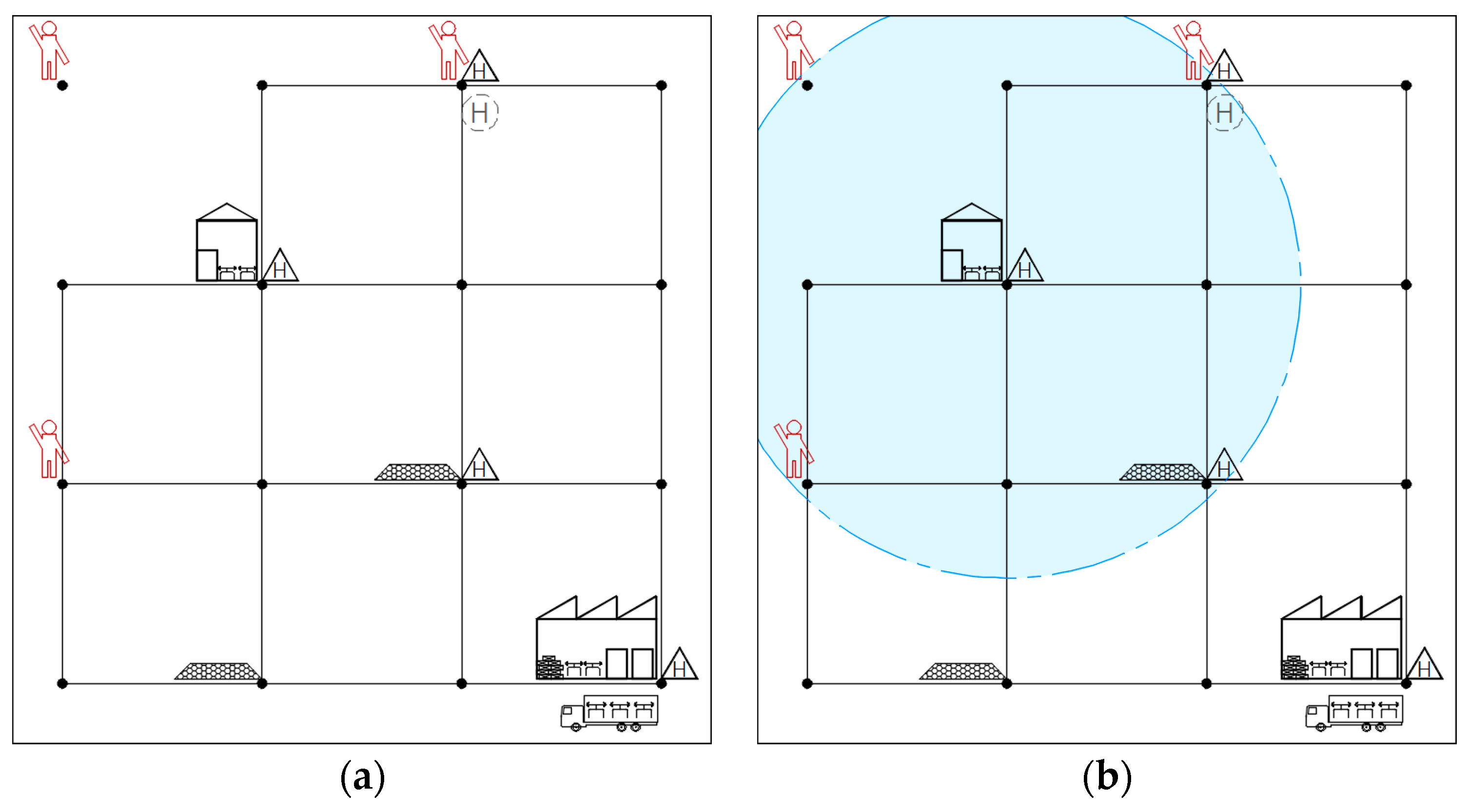
We are proposing a mix of variable launch sites for LARO, featuring different characteristics among them. Customer locations can be used for CV-based UAV deployment, if local conditions allow (space, safety, airspace restrictions, customer approval, etc.). Virtual Hubs, for example, open spaces, parking lots, etc., can also be used for CV-based LARO. In both of those cases, the CV must wait for all its UAVs to return. UAVs can also be deployed from the Central Depot at the start, without any CV involvement, but also at the end, receiving items from the CV. Remote Depots are another facility type where the CV can leave items for UAV delivery, and LARO is performed by the depot personnel. Not all LARO locations are necessarily used.

-

Deliveries can be made both by CV and UAV.

-

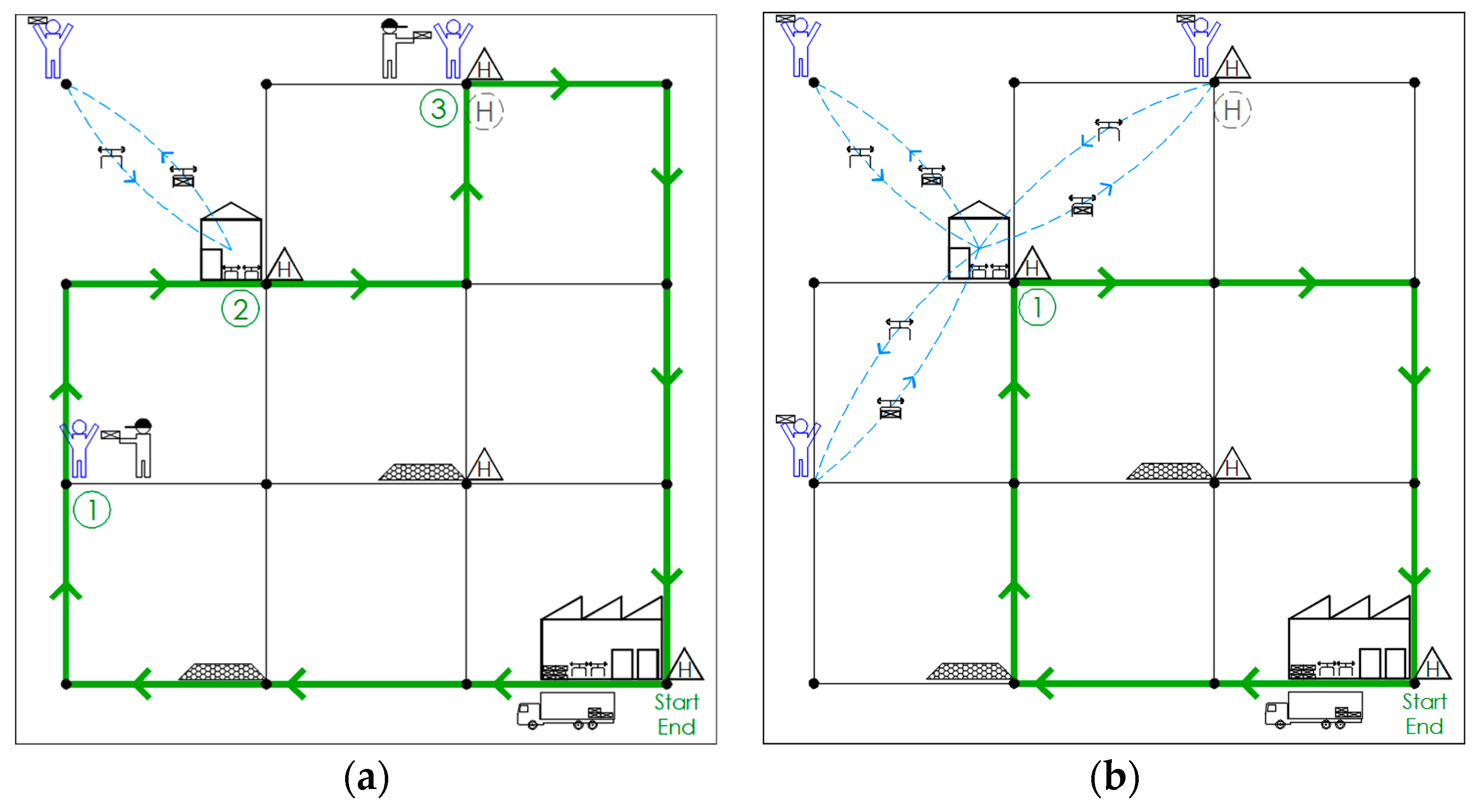
The CV network is available for routing and LARO, but not all nodes and links are necessarily used. We distinguish the mandatory nodes for actions and routing after the assignment process, creating the so-called “shell network”. This allows for our model to be practically implemented with different demands and infrastructure each time.

-

The Assignment and Routing Optimization nested GA is developed specifically for our problem, with its two steps being interconnected and using different methods for the inner and outer GA (discrete values resulting from the service nodes for the assignment process and random keys-based ordering of nodes for routing).

-

We have considered the presence of Restricted Zones of any shape and size and adjusted our model to filter out non-reachable locations, either because they are in such zones or because the resulting UAV paths are longer than the UAV range allows.

-

We are adjusting the model, incorporating spatial and optimal path analysis with GIS as part of the methodology, and opening to modern methods and input norms.

-

The formulation is conveniently simplified but unique to its kind since it must address the specific setup. It creates a modular and open platform that is open to modifications, and we present all the analytical calculations involved. This also helps with strategic planning, e.g., deciding where to establish Remote Depots or Virtual Hubs, by conveniently testing alternative locations.

-

The consideration of all the above in a single proposed method, in a comprehensive and holistic approach.

2. Materials and Methods

2.1. General Problem Description

Several items must be delivered from a Central Depot (CD) to customers at Delivery Locations (DLs). CVs travel through a fixed network, whereas UAVs are more flexible, although they are obliged to navigate around potential no-fly zones. The CV is not limited by its operational range and is expected to be able to complete the entire journey without refueling or charging. The UAVs are assumed to be electric, with battery capacity and energy consumption performance defining their maximum range. A battery swap is executed at the start of operations or during the UAV preparation at each site when the same UAV is used again. Each item is assigned to a mode for the final stretch or the entirety of the journey.

In our setup, UAVs can be launched or recovered at allowed locations throughout the network; these locations are not limited to the DLs or the CD, but additional Virtual Hubs (VHs) for convenient CV layover and in situ UAV deployment, and Remote Depots (RDs) with adequate UAVs are also available. When UAVs are deployed from the CD or the RDs, the CV does not have to wait for the UAVs to return. However, at RDs, a certain service time for item delivery is implied before the depot’s personnel assume the package mounting and UAV deployment activities. At any other location where UAVs are mass-deployed from the CV, the latter must wait for the last UAV to return. Under the given network and introduced demand and restrictions, the goal is to find the best combination of item assignment and CV routing in terms of the total time to complete operations. A simplified illustration of this setup is presented in the following figures (Figure 1, Figure 2 and Figure 3).

2.2. Assumptions and Constraints

Apart from the general description, certain assumptions and constraints need to be set to accurately describe the proposed delivery system:

• A single CV is available, departing from the Central Depot and attempting to deliver the items to their destinations.
• The CV is assumed to have adequate capacity for the items, and any UAVs may be needed onboard.
• Vertical Take-off and Landing (VTOL) UAVs are selected.
• Each destination can be visited once for delivery or UAV deployment (or both during the same stop) but can be accessed more than once for routing purposes.
• There is no predefined mode assignment for the items, but there is an option to force one if needed.
• There is no predefined order of visits for the destinations, but there is the option to force one if needed.
• The CD is the start and end node for the conventional vehicle tour.

We also assume the following:

• Each item is assigned to one vehicle (CV or UAV) for the final step of delivery.
• The CV can be assigned to multiple destinations.
• Each UAV has the capacity for one item.
• Each UAV can travel to and return from one destination per tour (the same UAV can be later re-deployed, but we have assumed enough UAVs for all operations anyway).
• UAVs can be deployed as a fleet from a single station.
• The launch of all UAVs from a launch site is simultaneous, but each one returns at a different time depending on the length of its tour.
• A UAV is recovered at the same location where it was launched.
• Remote Depots can deploy UAVs without the CV having to wait for their return. A certain amount of transshipment time is still required.
• The CD, used at the start of operations, can deploy UAVs without the CV having to wait, and no transshipment time is required.
• Only one transfer between vehicles is allowed per item.

We are proposing a framework that extends from inputs to analysis to solution methodology. Figure 4 below summarizes said framework and workflow until the final solution.

Basic information on the physical network acts as initial input (Conventional Vehicle Network, CVN), the infrastructure (Central Depot (CD), Remote Depot (RD), Virtual Hub (VH)), as well as equipment specifications (CV and UAV operational characteristics). Then certain locations (Delivery Locations (DLs)) represent demand for item deliveries.

Preliminary analysis defines which sites are finally allowed for UAV deployment (Launch Sites (LSs), among CD, RDs, VHs, and some of the DLs) and which pairs of DLs and LSs are within the maximum UAV range (straight flight path) of each other (DL_l^LS,max, LS_i^DL,max). For the above pairs, actual optimal paths around RZs are estimated, and UAV-feasible connections are again filtered based on the UAV’s range. Each item is then associated with potential service nodes (Service Nodes Pool (SN_k)). A service node for an item may be its own DL node (if within the CVN) or any allowed LS that is reachable by UAV. Analysis “a2” offers an alternative way to perform the assignment later (task T1). Instead of assigning items based on their Service Nodes Pool, we could inversely use the ${DL}_l^{LS}$ sets of the launch sites. This would be helpful if we were to base our assignment on clustering strategies.

To obtain the optimal solution, we are setting up a nested two-level optimization process, seeking the optimal assignment of items to a service node (l_k) and optimal CV routing. Each time an assignment iteration is produced, a set of mandatory nodes (T^v_M) for visit emerges. At each of these nodes, waiting times (wt_i) for the CV are calculated based on the actions required (e.g., in-person delivery, UAV launch and recovery, items delivered to an RD for UAV deployment by the personnel). The shortest paths ($\widehat{S_{ij}}$) between mandatory nodes are calculated using the given CVN and a new “shell” network is created. The shell network is constructed by a subset of mandatory nodes and the travel costs between them. Routing for the CV is then a matter of selecting the best order of visits ($\widehat{S_{ij}^M}$) across mandatory nodes. (In our case study experiments, we have opted to use the nested GA with a custom gene structure for tasks T1, T2, and an A* algorithm for the shortest path analysis s2.)

The target is to minimize Global Operations Time (GOT), the time needed for all vehicles (CV and deployed UAVs) to complete their tasks and return to their intended base.

2.3. Mathematical Formulation

We introduce a series of notations and variables, shown in

Table 1. Notations and terminology.

Abbreviations
CV: Conventional Vehicle (truck, train, vessel, here: truck) UAV: Unmanned Aerial Vehicle (aka drone) VTOL: Vertical Take-Off and Landing (UAV type) CVN: Physical (fixed) network of CV operation RZ: Restricted Zone (no-fly) CD: Central Depot, forming subset ${\mathit{T}}_{\mathit{C}\mathit{D}}^{\mathit{v}}$ CD′: Central Depot Duplicate, forming subset ${\mathit{T}}_{\mathit{C}{\mathit{D}}^{\mathbf{\prime }}}^{\mathit{v}}$ RD: Remote Depots, forming subset ${\mathit{T}}_{\mathit{R}\mathit{D}}^{\mathit{v}}$	VH: Virtual Hubs, forming subset $T_{VH}^v$ DL: Delivery Locations, forming subset $T_{DL}^v$ UL: UAV visitable DLs, forming subset $T_{UL}^v$ LS: Launch Sites, forming subset $T_{LS}^v$ SN: Service Nodes for item $CVT$: Total time of travel for the CV (since start) $GOT$: Global Operations Time, when all vehicles have completed their tasks and have returned to their intended base (since start)
Parameters
SCV′: CV mean speed SUAV: mean UAV speed at cruising altitude SUAVasc: mean UAV speed of ascend SUAVdes: mean UAV speed of descend	RUAV: UAV range of operation (time) HUAV: UAV cruising altitude ${tc}_i$: transshipment cost (time to deploy UAV) $st$: service time
Variables
${\mathit{x}}_{\mathit{i}}^{\mathit{C}\mathit{D}}$: Binary variable (0,1) indicating node type “Central Depot” ${\mathit{x}}_{\mathit{i}}^{\mathit{R}\mathit{D}}$: Binary variable (0,1) indicating node type “Remote Depot” ${\mathit{x}}_{\mathit{i}}^{\mathit{V}\mathit{H}}$: Binary variable (0,1) indicating node type “Virtual Hub” ${\mathit{x}}_{\mathit{i}}^{\mathit{D}\mathit{L}}$: Binary variable (0,1) indicating node type “Delivery Location” ${\mathit{x}}_{\mathit{i}}^{\mathit{L}\mathit{S}}$: Binary variable (0,1) indicating node type “Launch Site” ${\mathit{L}}_{\mathit{i}\mathit{j}}^{\mathit{C}\mathit{V}}$: Length of CVN edge ${\mathit{f}\mathit{t}}_{\mathit{i}\mathit{j}}$: UAV flight time at cruising altitude ${\mathit{L}}_{\mathit{i}\mathit{j}}^{\mathit{U}\mathit{A}\mathit{V}}$: Length of UAV edge, at cruising altitude $\mathit{t}\mathit{t}\mathit{a}$: Time to ascend (take-off to cruising altitude) $\mathit{t}\mathit{t}\mathit{d}$: Time to descend (cruising altitude to landing) ${\mathit{t}\mathit{f}\mathit{t}}_{\mathit{i}\mathit{j}}$: Total UAV airtime from take-off to landing ${\mathit{x}}_{\mathit{i}\mathit{j}}^{\mathit{U}\mathit{A}\mathit{V}}$: binary variable (0,1) for the existence of direct UAV connection (in range), $\mathit{j}\in \mathit{V},\mathit{i}\ne \mathit{j}$ ${\mathit{x}\mathit{d}}_{\mathit{i}}^{\mathit{C}\mathit{V}}$: binary variable (0,1) indicating final delivery with CV	$\left|L_l\right|$: number of items assigned to launch site ${dth}_{ij}$: time for UAV deployment-to-home ${wt}_i$: waiting time of CV on node $x_i^{CRD}$: binary variable (0,1) indicating whether a node is either type of depots ${ct}_{ij}^M$: cost (time) for shortest path between two mandatory nodes ${xa}_i$: binary variable for access of node by CV ${uf}_{ij}$: binary variable for edge traveled by UAV ${uv}_{ij}$: binary variable for edge traveled by CV ${pa}_{ij}$: cumulative passes over edge by CV $t_j^{app}$: time of CV approach to node $t_j^{dep}$: time of CV departure from node $t_l^{ret}$: time of return of last UAV, when the launch site is a depot (since start) ${dt}_k$: time of delivery of item (since start)

.

The fixed network that is traversable by the CV (Conventional Vehicle Network, CVN) is first introduced. Let it be an undirected graph, i.e., G′ = (V′, E′), where each vertex (“node”) belongs to the set:

V′ = [0, 1, 2, …, n]

(1)

Edges of the E′ [G′] space result from the connection between two nodes i and j, as e(i,j), belonging to the respective set:

E′ = {(i,j): i, j ∈ V′, i ≠ j}

(2)

A binary variable, $x_{ij}^{CV}$, shows whether a connection exists between two nodes for the CV.

$$x_{ij}^{CV}=\left\{\begin{array}{c}0,\hspace{1em}\hspace{1em}\hspace{1em}nodirectconnectionwithCV\\ 1,\hspace{1em}directconnectionavailablewithCV\end{array}\right.\hspace{1em}\hspace{1em}\hspace{1em}\hspace{1em}i,j\in V^{\prime }$$

(3)

A cost, ct_ij, is awarded to each edge; we will be using time since it is of primary concern in logistics operations and is also a common parameter between edges (travel times) and nodes (service and waiting times). The vehicle can travel an edge in both directions (an undirected graph).

$${ct}_{ij}=\raisebox{1ex}{$L_{ij}^{CV}$}\!\left/ \!\raisebox{-1ex}{$S^{CV}$}\right.,\hspace{1em}\hspace{1em}\hspace{1em}i,j\in V^{\prime }$$

(4)

• ‘L^CV_ij’: length of road link between points i and j
• ‘S^CV’: CV mean speed

Information on the types of CVN nodes follows. Several types are identified and can be passed on to the nodes: a Central Depot (CD), which is the starting point for the operations; Remote Depots (RDs), which can provide additional UAVs for delivery; and Virtual Hubs (VHs), which are designated safe areas for UAV deployment (e.g., parking lots, open spaces, organized launch/land bases). All others are considered generic nodes. Also, there is demand for deliveries at certain locations (Delivery Locations, DLs).

A list, “K”, of “m” items (each element: “k”) is given, along with their geographic position:

K = [1, 2, …, m]   (set of items)

(5)

A DL may not be reachable by CV at all, i.e., it may not belong to the CVN. A vertex set, “V”, is created, combining CVN and DL nodes ($V=V^{\prime }\cup \left[DL\right]$). The DL of each item is matched with a vertex of the “V” space and is then represented by it. The set of the respective nodes is defined as

$$C_k=\left[d_1,d_2,\dots ,d_m\right]=\left[DL\right]\hspace{1em}\hspace{1em}\hspace{1em}k\in K,C_k\subseteq V$$

(6)

For computational convenience, we introduce an expansion of the initial CVN graph including any DLs outside the CVN: G = (V, E), with E = {(i,j): i, j $\in$ V, i ≠ j}. Nodes outside the initial set V′ (resulting from DLs) would have no edge connection with any other node in V.

UAVs may launch and land at certain locations based on prevailing restrictions. Such locations are called Launch Sites (LSs), and they are potential points for launching and collecting UAVs. We also introduce a definition for DLs that are visitable by UAV, “UL”.

Based on the above, available special node types in the vertex set (V) may be:

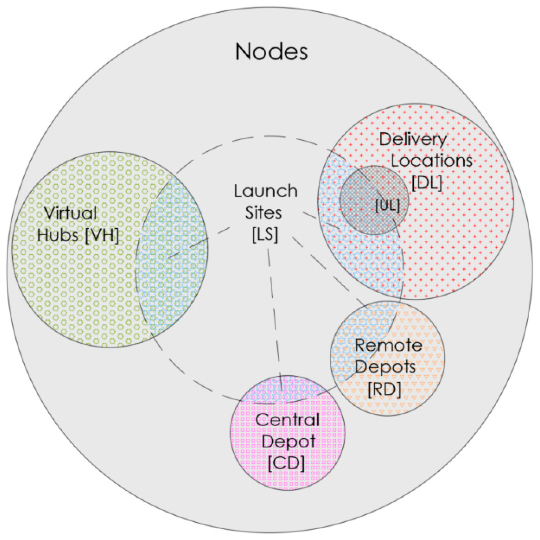
• Central Depots (CDs), forming a subset of vertices, $T_{CD}^v$, where $x_i^{CD}=1$. This subset here only contains one vertex, always named “0”.
• Remote Depots (RDs), forming a subset of vertices, $T_{RD}^v$, $x_i^{RD}=1$. An RD may be a designated location with available UAVs to deploy. As such, a Conventional Vehicle will not have to carry UAVs onboard or wait for any deployed UAVs to return.
• Virtual Hubs (VHs), forming a subset of vertices, $T_{VH}^v$, $x_i^{VH}=1$. A Virtual Hub is an initially designated location throughout the conventional network where conventional vehicles are allowed to deploy UAVs (e.g., parking lots, special bases for take-off and landing).
• Delivery Locations (DLs), forming a subset of vertices $T_{DL}^v$ ($T_{DL}^v=C_k)$, $x_i^{DL}=1$. A Customer Location is a point of demand for a specific item delivery, item collection, or service. UAV-visitable locations (UL) form an additional subset among DLs, $T_{UL}^v$, $x_i^{UL}=1$.
• Launch Sites (LSs), forming a subset of vertices $T_{LS}^v$, $x_i^{LS}=1$. A Launch Site is ultimately a location where a UAV can be launched or collected, depending on circumstances (UAV range and DL location, flight restrictions, weather, other temporary technical issues). CD, RDs, VHs, and DLs may be Launch Sites or not. A Launch Site is an “allowed” site for launch or collection.

Launching and collecting a UAV is possible in other locations than just the CD and DLs. Additionally, not all DLs are potential LSs. This is different from the assumption commonly made in the literature about cooperative truck–drone systems, where drones can only fly from or to customer locations or the CD. A schematic representation of node sets is shown in Figure 5.

For computational reasons, a duplicate node of the CD (CD’), forming a set $T_{C{D}^{\prime }}^v$, is created, along with its associated edges, only this time it is characterized as an RD. This serves to cater to a generalized case of using the CD for UAV deployment at the end of the CV route rather than at the start of operations.

For UAV operations, we define an undirected graph, F = (V, A). Edges of the A[F] space result from the connection between two nodes i and j, as a(i,j), belonging to the set:

A = {(i,j): i, j ∈ V, i ≠ j}

(7)

We assume typical UAV VTOL behavior, which implies an initial vertical ascent to the cruising altitude and finally a vertical descent to the landing position. Figure 6 illustrates the flight pattern suggested.

The UAV can operate within a certain range, defined by its specs and battery, which is usually expressed in time. The following parameters regarding the UAV are defined: mean cruise speed (S^UAV), mean speed of ascend (S^UAV_asc), mean speed of descend (S^UAV_des), range of operation (time) (R^UAV), and cruising altitude (H^UAV).

Flight time “ft_ij” is the time needed for a UAV to fly from location “i” to location “j” at cruising altitude. This is essentially the weight (in time) of an edge if traveled by UAV. We assume a symmetric problem for the UAV operations, i.e., ft_ij = ft_ji.

$${ft}_{ij}=\raisebox{1ex}{$L_{ij}^{UAV}$}\!\left/ \!\raisebox{-1ex}{$S^{UAV}$}\right.,\hspace{1em}\hspace{1em}i,j\in V$$

(8)

• ‘L^UAV_ij’: distance between points i and j
• ‘S^UAV’: UAV mean flight speed

“Time to ascend” (tta) and “time to descend” (ttd) values are considered. Considering only direct flights between nodes (no stops at other nodes), the total flight time “tft_ij” between two points is calculated as

$${tta}_i=\raisebox{1ex}{$H^{UAV}$}\!\left/ \!\raisebox{-1ex}{$S_{asc}^{UAV}$}\right.\hspace{1em}\hspace{1em}\hspace{1em}\hspace{1em}\hspace{1em}{ttd}_i=\raisebox{1ex}{$H^{UAV}$}\!\left/ \!\raisebox{-1ex}{$S_{des}^{UAV}$}\right.$$

(9)

$${tft}_{ij}={tta}_i+{ft}_{ij}+{ttd}_j$$

(10)

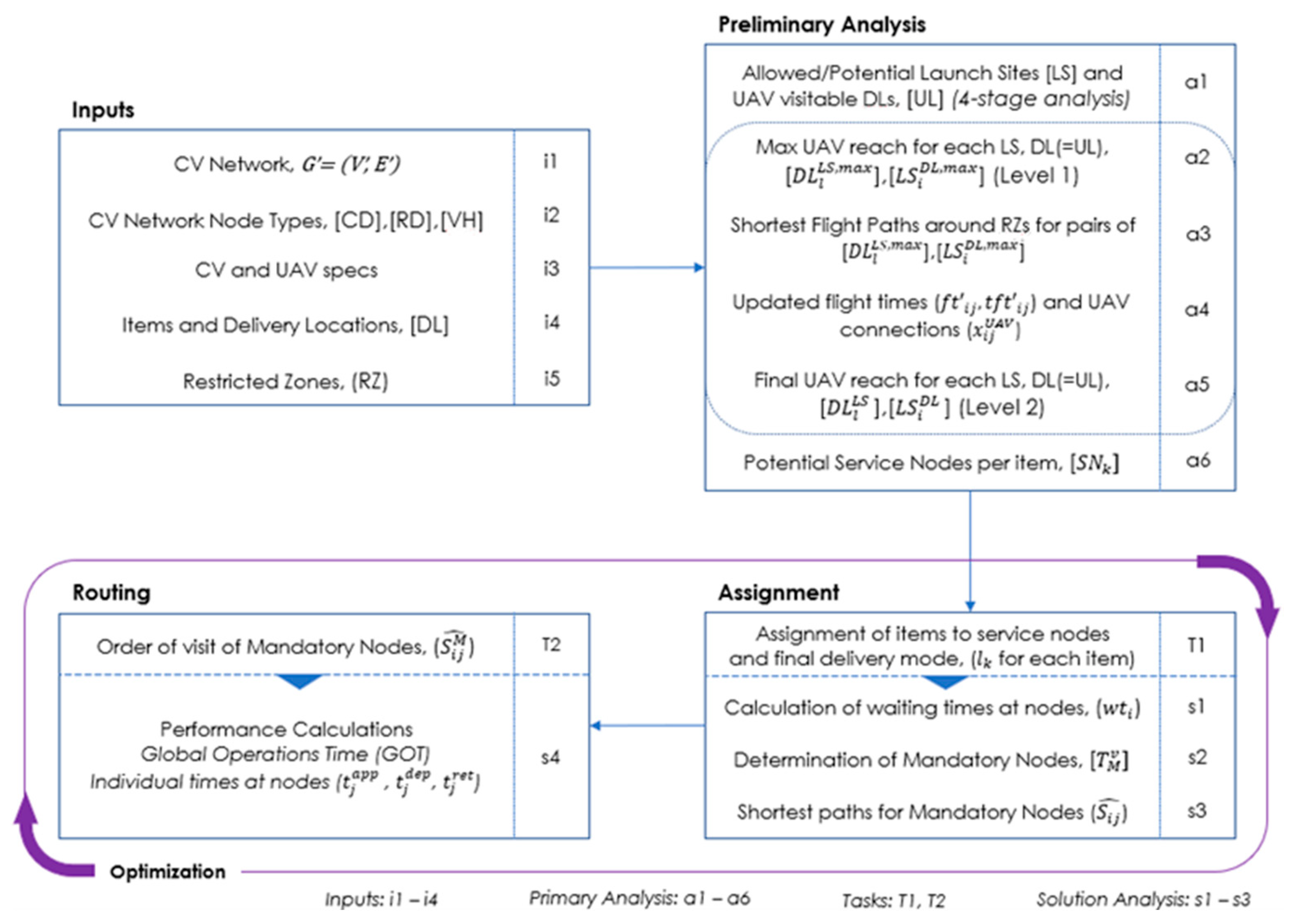
2.4. Preliminary Analysis

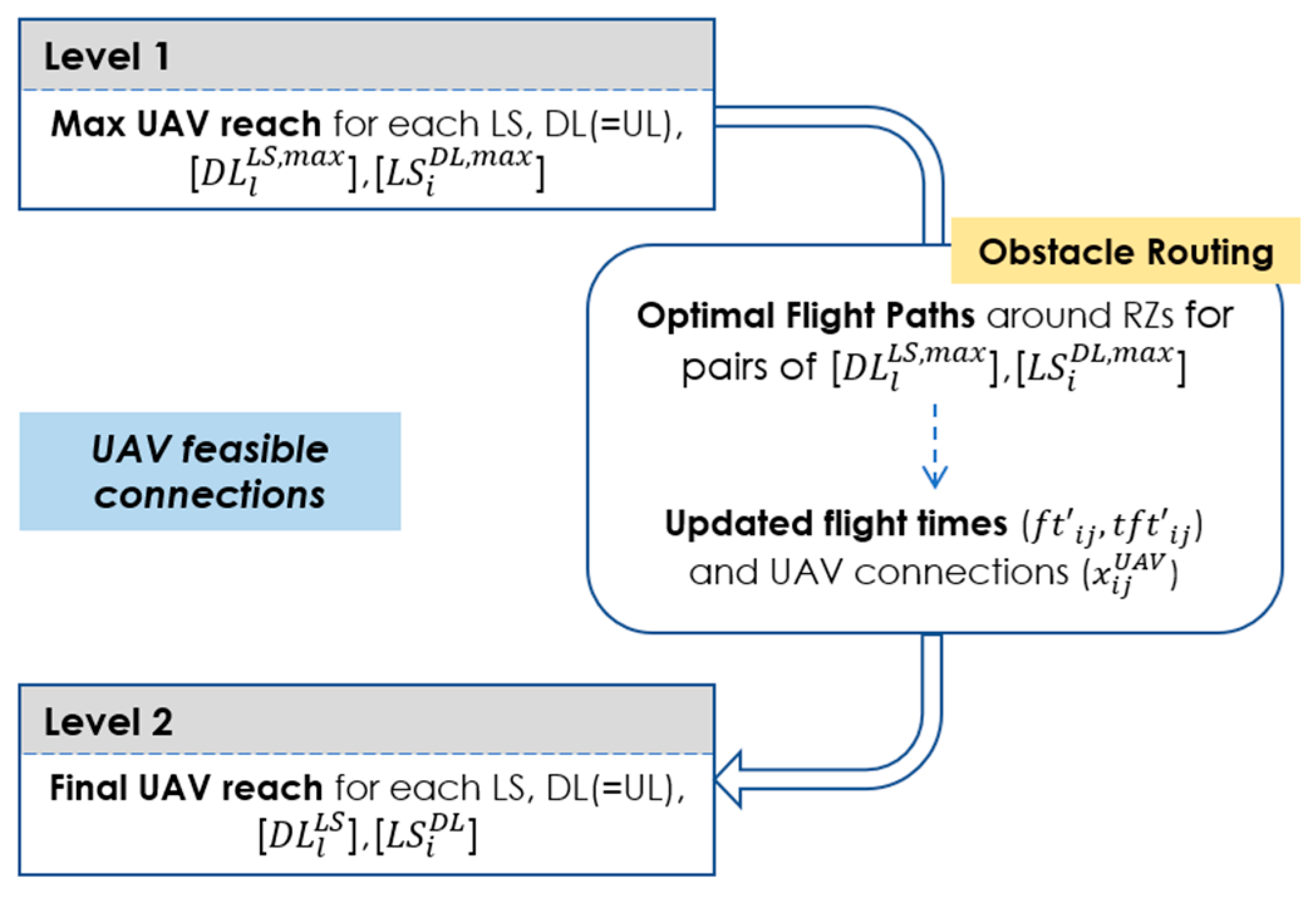
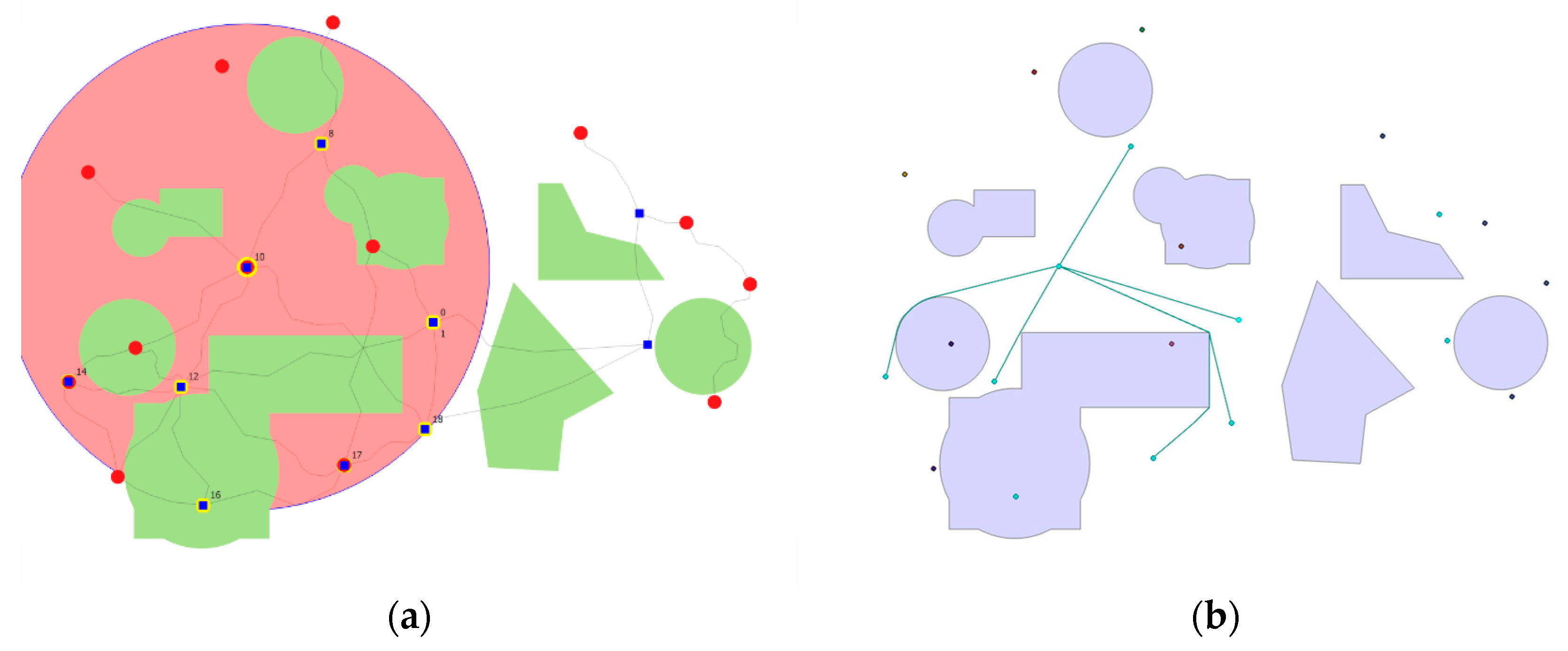
2.4.1. UAV Range and Connections

One of the most important processes within the proposed workflow is the identification of the allowed LSs and UAV-visitable DLs. This is executed in stages as new information emerges.

• Stage 0: Initial Infrastructure (CD, RDs, VHs);
• Stage 1: Physical constraints on emerging DLs (e.g., area characteristics, obstacles, safe room for take-off and landing);
• Stage 2: Operational constraints (e.g., maintenance, time of day, customer choices)
• Stage 3: RZ constraints (an LS or DL falls within an RZ).

Stage 3 analysis assumes that any location “i” falling within an RZ cannot be an LS or UL; thus, $x_i^{LS}=x_i^{UL}=0$.

To reduce the computational burden, pre-processing for feasible UAV connections may be performed only for nodes of interest, that is, the Launch Sites $\left(T_{LS}^v\right)$ and eligible Delivery Locations $\left(T_{UL}^v\right)$. As with the CV, we define a binary variable, $x_{ij}^{UAV}$, representing a direct connection between two nodes, for the case of the UAV.

The existence of a direct UAV connection between two nodes is determined by the range, “R^UAV”, of the UAV and/or extraordinary conditions (e.g., takeoff and landing restrictions, air traffic rules, weather).

$$x_{ij}^{UAV}=\left\{\begin{array}{c}0,\hspace{1em}\hspace{1em}\hspace{1em}\hspace{1em}{tft}_{ij}{+tft}_{ji}>R^{UAV}\\ 1,\hspace{1em}\hspace{1em}0<{tft}_{ij}+{tft}_{ji}\le R^{UAV}\end{array}\right.\hspace{1em}\hspace{1em}\hspace{1em}i,j\in V,i\ne j$$

(11)

Based on the above analysis, for each Launch Site and Delivery Location, a set of reachable nodes is formed. The analysis is performed at two levels. First, the maximum reachable DLs and LSs are identified, assuming no air space restrictions and straight-line paths between node pairs.

$$\begin{gathered} {DL}_l^{LS,max}=\left[A\subseteq V|x_{li}^{UAV}=1,\hspace{1em}\hspace{1em}i\in UL,l\in LS\right] \\ \left(\text{Delivery Locations, visitable by UAV, within range of the Launch Site}\right) \end{gathered}$$

(12)

$$\begin{gathered} {LS}_i^{DL,max}=\left[B\subseteq V|x_{il}^{UAV}=1,\hspace{1em}\hspace{1em}i\in UL,l\in LS\right] \\ \left(\text{Launch Sites within range of the Delivery Location that are visitable by UAV}\right) \end{gathered}$$

(13)

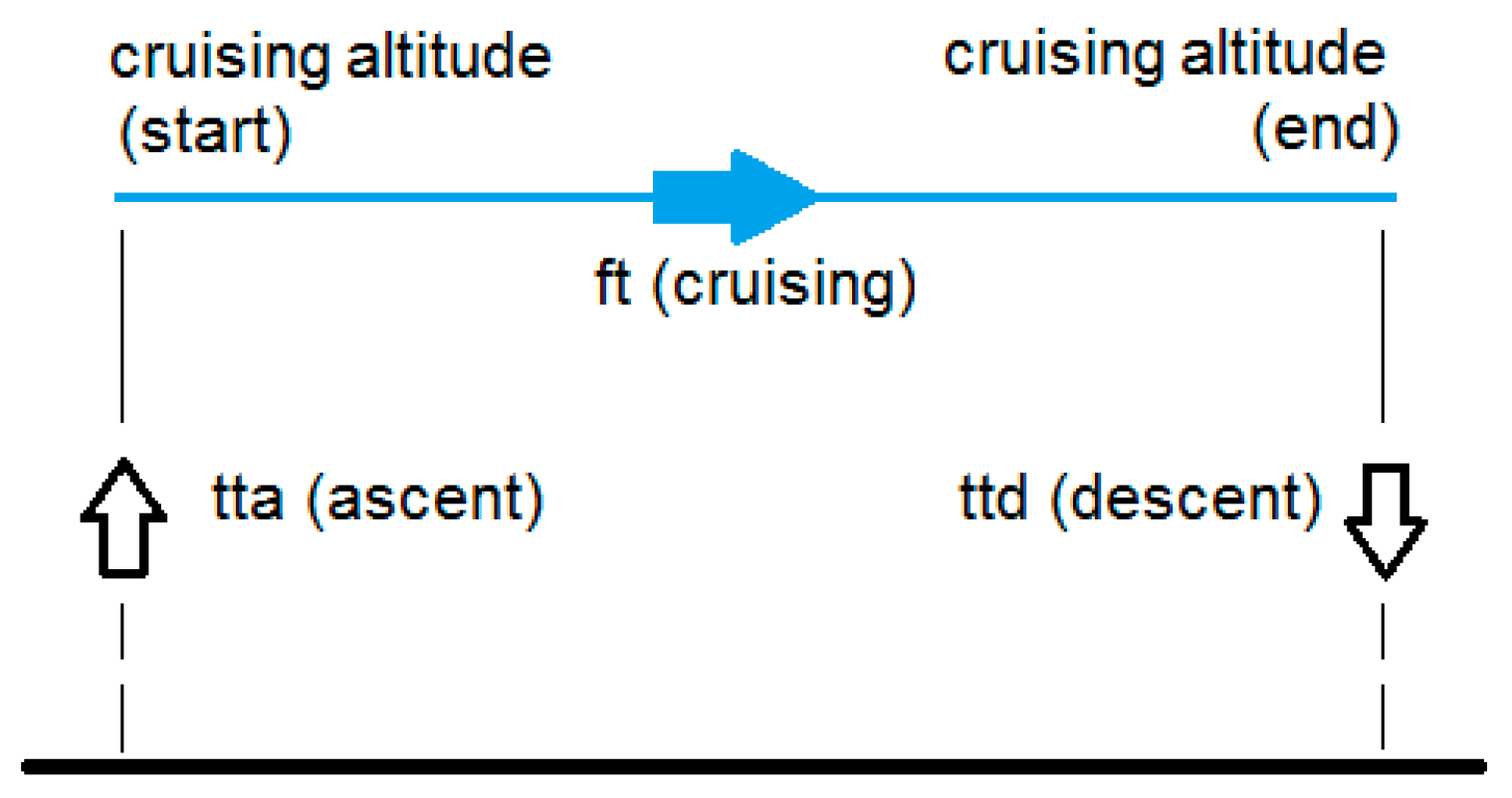
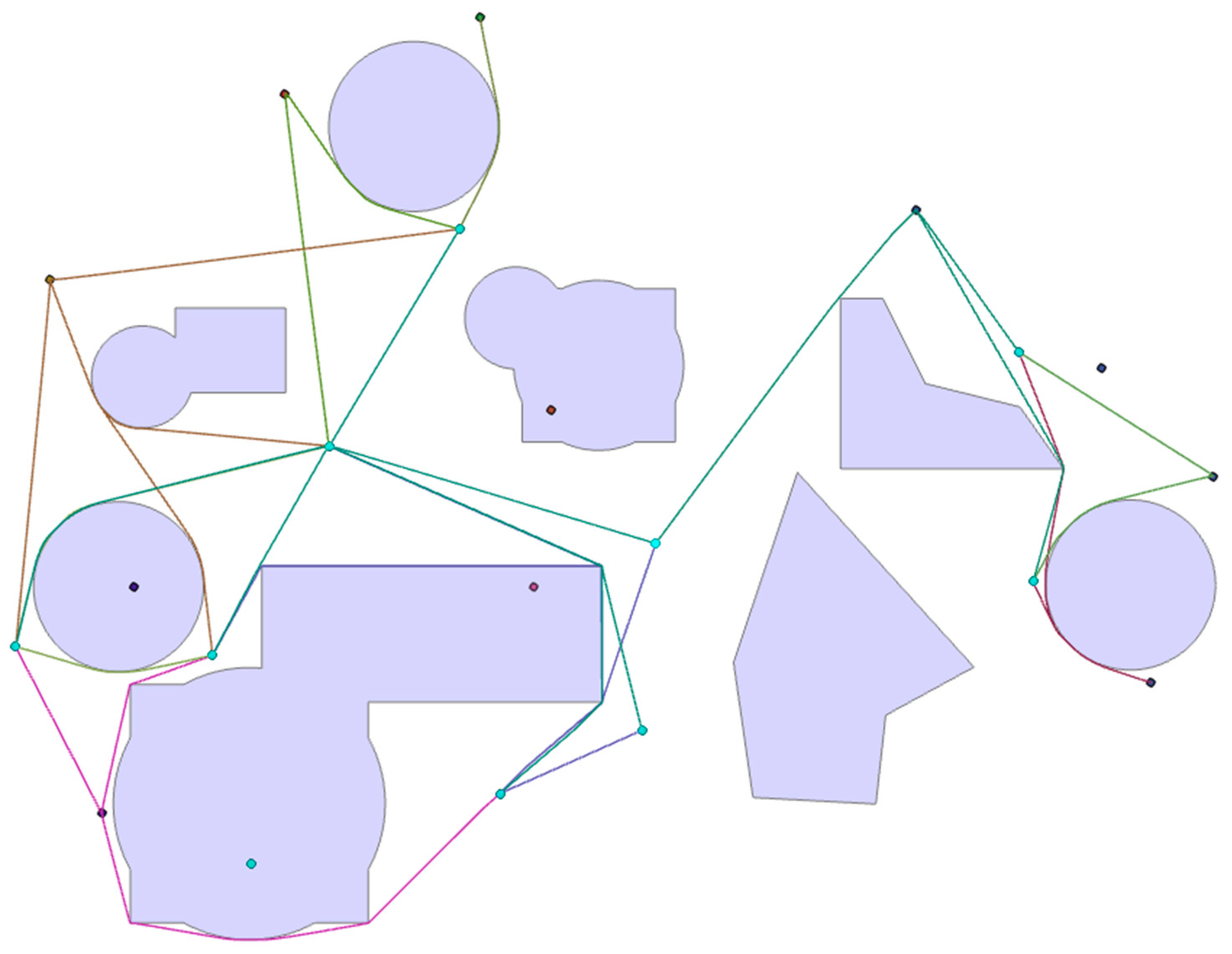
2.4.2. Obstacle Routing and Flight Time Updates

The actual flight paths around RZs are calculated only for the pairs resulting from the first level of filtering for DLs and LSs (${DL}_l^{LS,max},{LS}_i^{DL,max}$), since there is no possibility for other pairs to have feasible UAV connections. Acquiring optimal paths around obstacles is an intensive process. By first applying the Level 1 filter, which is simple and quick, the overall computational effort is significantly reduced. Figure 7 explains the proposed two-level process for finalizing the UAV edge weights and the reachable LSs for each DL.

We employ a suitable algorithm for obtaining optimal paths around the RZs. Source and target nodes are feasible LS and DL pairs that have resulted from the first-level Level analysis.

New values for flight time and total flight time (${f{t}^{\prime }}_{ij}$ and ${tf{t}^{\prime }}_{ij}$, respectively) emerge based on the length of the new flight paths. The edges a(i,j) of graph F = (V, A) are updated, responding to ${tf{t}^{\prime }}_{ij}$. The values $x_{ij}^{UAV}$ are also updated based on the new flight times between nodes:

$$x_{ij}^{UAV}=\left\{\begin{array}{c}0,\hspace{1em}\hspace{1em}\hspace{1em}\hspace{1em}{tf{t}^{\prime }}_{ij}+{tf{t}^{\prime }}_{ji}>R^{UAV}\\ 1,\hspace{1em}\hspace{1em}0<{tf{t}^{\prime }}_{ij}+{tf{t}^{\prime }}_{ji}\le R^{UAV}\end{array}\right.\hspace{1em}\hspace{1em}\hspace{1em}\hspace{1em}\hspace{1em}i,j\in V,i\ne j$$

(14)

The final lists of reachable LSs and DLs are calculated:

$$\begin{gathered} {DL}_l^{LS}=\left[A\subseteq V|x_{li}^{UAV}=1,\hspace{1em}\hspace{1em}i\in UL,l\in LS\right] \\ \left(\text{Delivery locations, visitable by UAV, within range of launch site}\right) \end{gathered}$$

(15)

$$\begin{gathered} {LS}_i^{DL}=\left[B\subseteq V|x_{il}^{UAV}=1,\hspace{1em}\hspace{1em}i\in UL,l\in LS\right] \\ \left(\text{Launch sites within range of the delivery location that are visitable by UAV}\right) \end{gathered}$$

(16)

Since all UAV-related calculations will be based on the actual flight paths around obstacles, we can substitute respective values as follows: ${{ft}_{ij}=f{t}^{\prime }}_{ij}$, ${tft}_{ij}={tf{t}^{\prime }}_{ij}$. Each time a package is delivered to a location, a certain service time on the spot is considered. We assume a similar service time for both delivery via conventional vehicle and UAV, “st”.

A delivery request can be served by CV (at the node of said request) or by UAV (launching from another node among eligible launch sites). A pool of eligible service nodes can be defined for each item, containing the launch sites within range of the delivery location and the node of the delivery location itself. If the DL is not part of the original CVN, its own node cannot be part of this pool, ${SN}_k$.

$${SN}_k={LS}_{d_k}^{DL}\cup d_k,\hspace{1em}\hspace{1em}k\in K,d_k\in V^{\prime }$$

(17)

A DL may be non-serviceable. This happens when it is located outside the CVN, i.e., no CV can reach this destination, and at the same time, no allowed LS is located within the UAV range. In our algorithm, this state is plainly described by an empty SN_k pool. In this case, the DL is removed from demand.

2.4.3. Mode Assignment and Vehicle Routing

Having determined the potential LSs for all delivery locations, the assignment of each item to a UAV or CV follows. If the item is assigned to a node (let it be “$l_k$”) other than its own ($d_k$), the request is executed via UAV. If an item is assigned to its own node ($l_k=d_k$), the delivery is made by the CV.

We use the binary variable “${xd}_i^{CV}$” to define whether a delivery is made by a conventional vehicle at a node or not.

These nodes form a subset of “delivery with CV”:

$$T_{DLCV}^v=\left[DLCV\subseteq V|{xd}_i=1,i\in DL\right]$$

(18)

We also introduce another binary variable, “xl_i”, to define whether a node is ultimately used for UAV launch or not. These nodes must belong to the CVN.

Nodes form a subset of “assigned launch sites”:

$$T_{aLS}^v=\left[aLS\subseteq V|{xl}_i=1,i\in LS\right]$$

(19)

Nodes finally assigned as service nodes for either action (UAV launch or CV delivery) are Mandatory Nodes with Action(s) (item delivery or UAV launch), named “TMa”. The CV must visit them at some point along the route and perform an action other than just passing by.

$$T_{M\alpha }^v{=T}_{DLCV}^v\cup T_{aLS}^v$$

(20)

In our method, this distinction between generic and mandatory nodes is crucial. This is because the full network is given, but not all nodes must be visited, and the problem changes depending on infrastructure, conditions, equipment constraints, and demand. The full set of mandatory nodes results from the union of the two sets: $T_{DLCV}^v$ (delivery locations served by conventional vehicle) and $T_{aLS}^v$ (assigned launch sites), and the CD (which must be the first and last node to be visited, hence the inclusion of its duplicate):

$$T_M^v=T_{CD}^v{\cup T}_{M\alpha }^v{\cup T}_{C{D}^{\prime }}^v$$

(21)

There is a possibility of the CD or its duplicate being nodes with action (belonging to the $T_{M\alpha }^v$). We define a “clean” set, $T_{Mc}^v$, excluding the CD and CD’, as

$$T_{Mc}^v=T_M^v-\left(T_{CD}^v+T_{C{D}^{\prime }}^v\right)$$

(22)

We keep track of the items assigned to the same launch site for UAV delivery. As such, each node belonging to the $T_{aLS}^v$ will feature a list of the assigned items. A respective list is formed for each of the assigned launch sites:

$$L_l\subseteq K|l_k=l,l\in T_{aLS}^v,k\in K$$

(23)

The number of assigned items per launch site is the length of the list: $\left|L_l\right|$.

The use of a node as an LS implies a certain time cost (transshipment cost). This is because of the necessary preparations for UAV deployment. We include this transshipment cost in a variable called “tc_i”. UAVs are assumed to launch simultaneously, but they naturally return at a different time.

When a UAV is deployed, a certain amount of time is required for it to return to its base. This travel time, from deployment at node “i”, delivery at node “j”, and back to home “i”, “${dth}_{ij}$”, is calculated as

$${dth}_{ij}={tft}_{ij}+{st}_j+{tft}_{ji}$$

(24)

At every node, a certain waiting time, “wt_i”, for the CV is considered. Each node “i” inherits the “burden” of assigned delivery locations. If item delivery is its only duty at the node, this time is essentially the service time. If the spot is used for UAV deployment, the waiting time is also a result of the transshipment time for each item and the time from deployment to the home of the last UAV to return. If the aLS is an RD, the node is only weighted by the delivery of an item via CV (if any) and the time to unload the rest of the items for UAV transport. The typical service time, st_i, is used for unloading, as if it were a case of normal deliveries. However, we assume that service times here are affected by the number of unloaded items, as they would be for multiple deliveries on the spot. At depots, the transshipment cost does not affect the CV.

$${wt}_i={xd}_i^{CV}\cdot {st}_i+\left(1-x_i^{CRD}\right)\cdot {xl}_i\cdot \left[{\left|L_i\right|\cdot tc}_i+\max \left({dth}_{ij}\right)\right]+x_i^{RD}\cdot {xl}_i\cdot \left|L_i\right|\cdot {st}_i$$

(25)

$${x_i^{CRD}=x}_i^{RD}+x_i^{CD},\hspace{1em}i\in V^{\prime },j\in L_i$$

(26)

For the special case of the CD, since there is no CV delivery and there is no unloading time for any UAV-assigned item, the CV does not have to wait, and everything is processed independently. Any UAV deployment from the CD would normally happen at the start of the operations, but we will also be allowing the CD to host actions as the last node of the tour. The CD duplicate (used as the last node of the tour) carries the characteristics of an RD to emulate the expected procedure of item unloading and UAV deployment.

Sub-Paths between Mandatory Nodes

In our case, where most network types should be addressed, typical TSP constraints restricting multiple node/edge passes and forcing the use of all nodes do not apply since not all nodes are mandatory and both butterfly routes and multiple node/edge passes are allowed (e.g., because of network dead ends or reaching a node for delivery or launch and immediately returning from the same road). We structure our method in such a way that it is not hampered by infeasible solutions: All mandatory nodes are always included in the solution (at least once for completing an action), and path continuity is ensured.

For assessing the performance of each solution, a certain route must be constructed, passing through the mandatory nodes and any other nodes necessary to form a continuous path. We will base this two-step method on the principle of optimality, stating that “in a graph with no negative dicycles, optimal paths must have optimal subpaths” [24]. We define a subgraph of the original G graph, $G_M=\left(T_M^v,E_M\right)$. Mandatory nodes (resulting from the assignment process) form the node set $T_M^v$. Each edge, $e_M$, is a “shell” edge, representing the shortest path between two nodes through the original network. For each $i,j\in T_M^v,i,j\in V^{\prime }$, there is a path of nodes $\widehat{S_{ij}}=\left[i,\dots ,j\right]$ and edges $\widehat{S_{\left(i,j\right)}}=\left[\left(i,i+1\right),\dots ,\left(j-1,j\right)\right]$, and the cost of the shell edge is

$${ct}_{ij}^M=\sum _{u=i}^{j-1}\sum _{v=u+1}^j{ct}_{uv}$$

(27)

The shortest path can be calculated via an appropriate algorithm each time (e.g., Dijkstra [37], A* [38], IDA* [39], LPA* [40]), depending on the complexity and size of the network.

Now, a certain sequence of visits must be defined through the mandatory nodes. The path always features the CD as the first and last node of visitation. As explained before, the CD’s duplicate visited at the end is considered an RD.

After decomposing the solution route to the nodes forming its shell edges, we have the order of visit of all nodes. The selected nodes constitute a subset, $T_{ACCV}^v$, with each one characterized by the binary variable xa_i.

The nodes are appended in the order of visits within the subset. This subset ultimately describes the problem’s possible solution each time. A node may be traversed more than once and may be repeated in the sequential order of visits. However, actions of delivery and/or launch only happen once.

If an edge is ultimately used by the conventional vehicle or the UAV, there is a binary variable to keep track of (uv_ij and uf_ij, respectively).

Since in our accepted spectrum of network types and based on our problem definition, it is possible that a CV edge is traversed more than once, we keep a record of the cumulative passes over each edge along the tour under the variable ${pa}_{ij}\in \mathbb{Z}$.

2.4.4. Objective Function and Solution Performance Calculations

For each node, there is a time of approach “$t_i^{app}$” since the start of delivery. Travel times along the selected edges of the conventional vehicle network are added, as are waiting times at preceding nodes.

Additionally, depending on which actions are taken (delivery at the node, deployment of UAVs), there is a time of departure, “$t_j^{dep}$”, at each node visited by the CV. In this case, the nodes of visitation are ordered.

$$t_j^{app}=\sum _{i=0}^j\sum _{j=0}^j{ct}_{ij}^M+\sum _{i=0}^{j-1}{wt}_i$$

(28)

$$t_j^{dep}=t_j^{app}+{wt}_j,\mathrm{or}{t}_j^{app}=t_{j-1}^{dep}+{ct}_{j-1,j}^M,i,j\in T_M^v$$

(29)

In case of a depot, the UAVs will be returning to their base independently from CV operations. We still need to know when the last one returns to the depot. The time of return should be

$$t_l^{ret}=t_l^{dep}+{\left|L_i^k\right|\cdot tc}_i+\max \left({dth}_{ij}\right),l\in T_{CD}^v\cup T_{RD}^v\cup T_{C{D}^{\prime }}^v,j\in L_l$$

(30)

Two values regarding the entire operation are of importance: the amount of time spent out for the CV and the entire time spent until any operation (CV or UAV) has finished. CV total time (CVT) is

$$CVT=\sum _{i=0}^n\sum _{j=0}^n{{pa}_{ij}\cdot ct}_{ij}+\sum _{i=0}^n{wt}_i$$

(31)

This value should be identical to the time of approach, $t_j^{app}$, at the last node.

If we were to optimize based on the CVT only, the routing of each assignment iteration would essentially be a form of TSP problem among mandatory nodes with weights. It is possible, however, that UAVs are still operating even after the CV has completed its own route. All operations are finished when the CV has returned to the depot and the last remaining UAV has been retrieved at the intended location. This is defined as Global Operations Time (GOT):

$$GOT=\mathrm{m}\mathrm{a}\mathrm{x}\left(\max \left(t_l^{ret}\right),CVT\right),l\in \left[CD\right]\cup \left[RD\right]$$

(32)

We use the GOT as the objective function, and the goal is to find a solution that minimizes its value.

$$\begin{gathered} \mathrm{Minimize}\mathrm{m}\mathrm{a}\mathrm{x}\left(\max \left(t_l^{ret}\right),CVT\right),\mathit{or}\mathit{alternatively}: \\ \mathrm{M}\mathrm{i}\mathrm{n}\mathrm{i}\mathrm{m}\mathrm{i}\mathrm{z}\mathrm{e}:\mathrm{m}\mathrm{a}\mathrm{x}\left(\max \left(t_l^{ret}\right),\sum _{i=0}^n\sum _{j=0}^n{pa}_{ij}\cdot {ct}_{ij}+\sum _{i=0}^n{wt}_i\right) \end{gathered}$$

(33)

The description of the solution output includes the following minimum information:

• The assignment of items to their respective service node ($l_k$ for each k);
• The order of visit of mandatory nodes (ordered set of $T_M^v$).

2.5. Proposed Solution Optimization Methodology

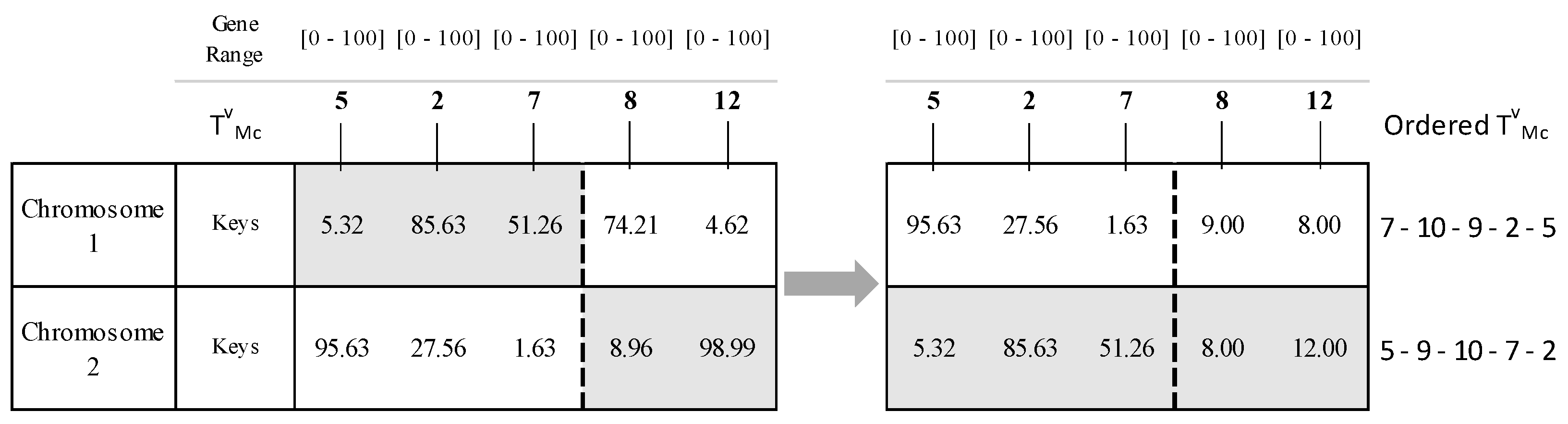
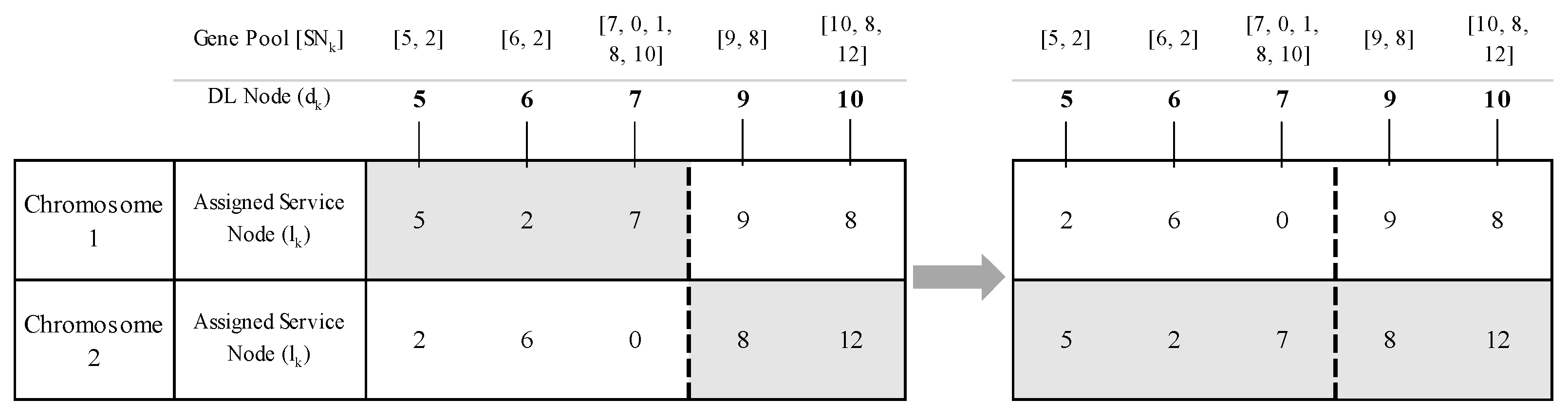
2.5.1. Assignment and Routing Optimization Nested Genetic Algorithm

We propose a nested Genetic Algorithm (GA) scheme where a routing optimization algorithm (inner GA) is executed for each assignment suggestion and the resulting GOT value is used to select the best assignment (shell GA). It is essentially a cluster-first, routing-second approach, where each clustering iteration is tied to its own optimal routing. GA-based methods are commonly used in this family of problems [52], mainly because of their NP-hardness and complexity [53]. In our case, preliminary processing produces discrete alternatives (Service Nodes Pool) for the assignment of items and a subset of nodes that need to be ordered. Both are conveniently translated to genes and chromosomes. Additionally, one process essentially depends on the other (routing is applied to mandatory nodes that result from assignment); thus, a nested scheme makes sense.

Outer GA (Mode and Service Node Assignment of Items)

For the outer GA, the chromosome consists of genes, whose total number equals the number of items, $m=\left|K\right|$, (delivery locations). Each gene can take the discrete values of the available service nodes (${SN}_k$) for the respective DL. Random mutation and single-point crossover are employed to produce new offspring and a ranking parent selection is used to qualify the best parents for mating. An example of the above gene structure for the outer GA (mode assignment) is shown in Figure 8.

Random mutations are introduced to genes to keep diversity in the population and escape local optima.

Inner GA (Conventional Vehicle Routing)

For the inner GA, we need to find the optimal order of visits to the mandatory nodes. Since the CD and its duplicate will always be the first and last nodes, respectively, the chromosome features genes, one for each of the mandatory nodes, without the start and end nodes, $T_{Mc}^v$. We employ a random-keys GA [24], where each node is ordered in ascending order based on its respective gene value. The gene values are randomly produced within a set range (e.g., 0–100). Single-point crossover and ranking parent selection are used. The final path begins and ends with the CD (its duplicate at the end), and in between there are the ordered nodes resulting from the previous process. The GOT value resulting from routing is passed to the respective outer GA iteration and used for its own optimization process. An example of the above gene structure for the inner GA (CV routing) is shown in Figure 9.

Again, random mutations are introduced to genes to keep diversity in the population and escape local optima.

3. Application and Results

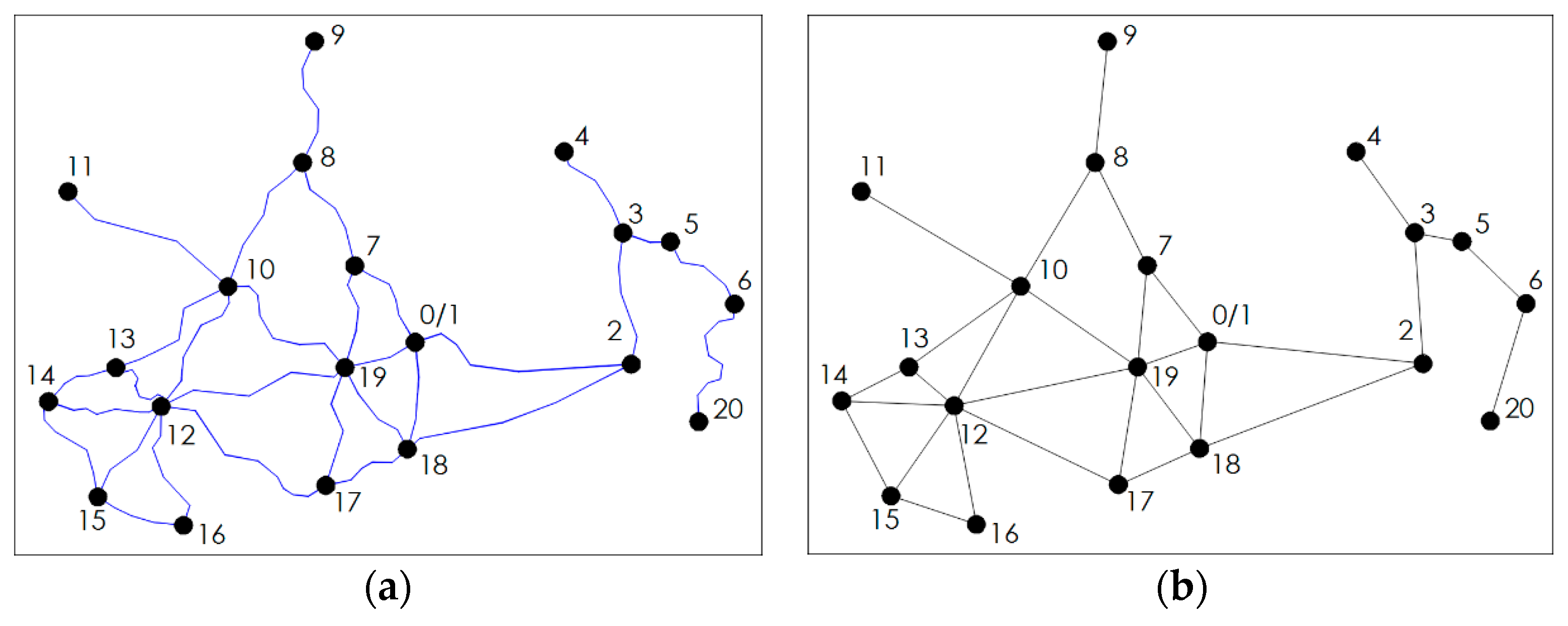
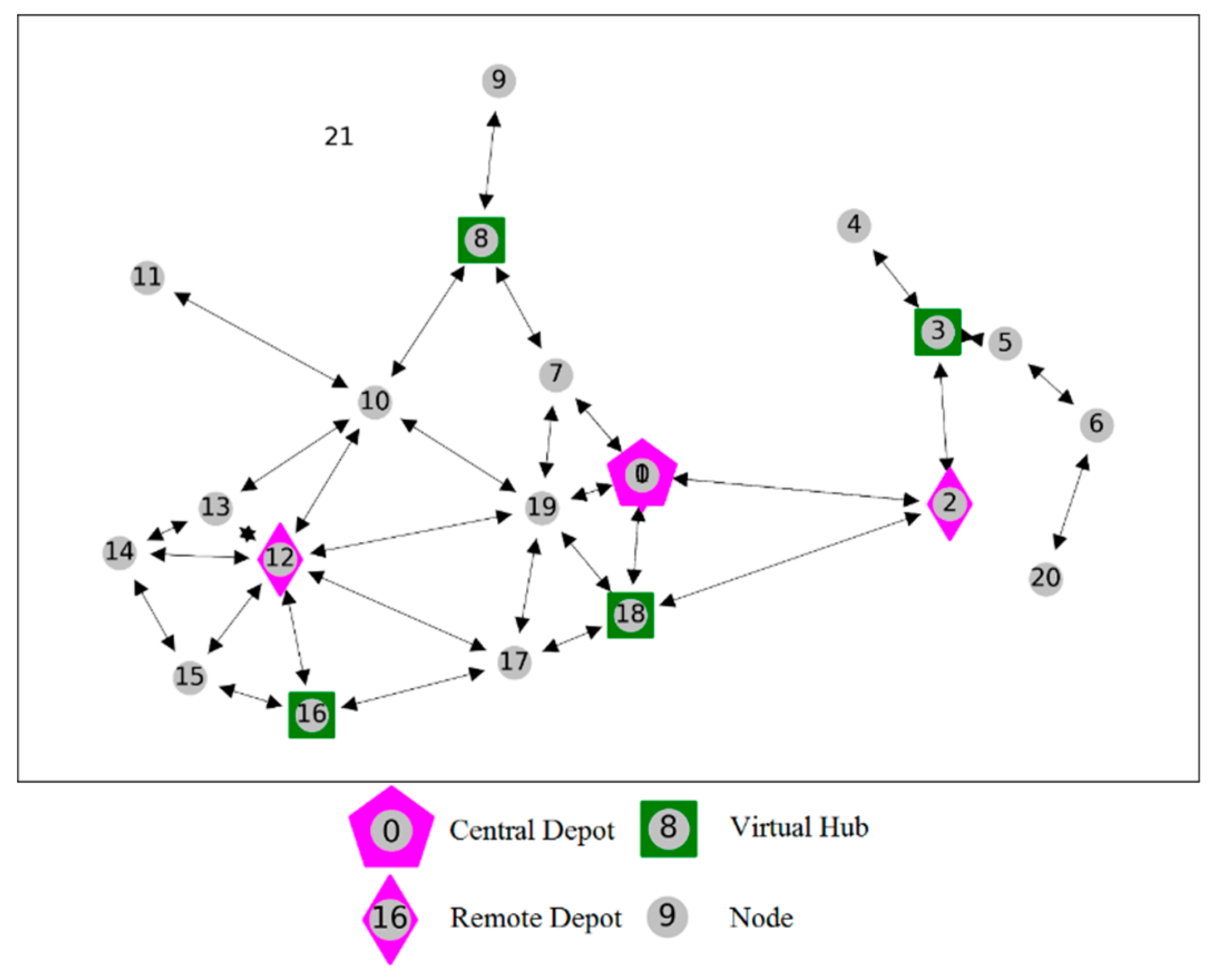
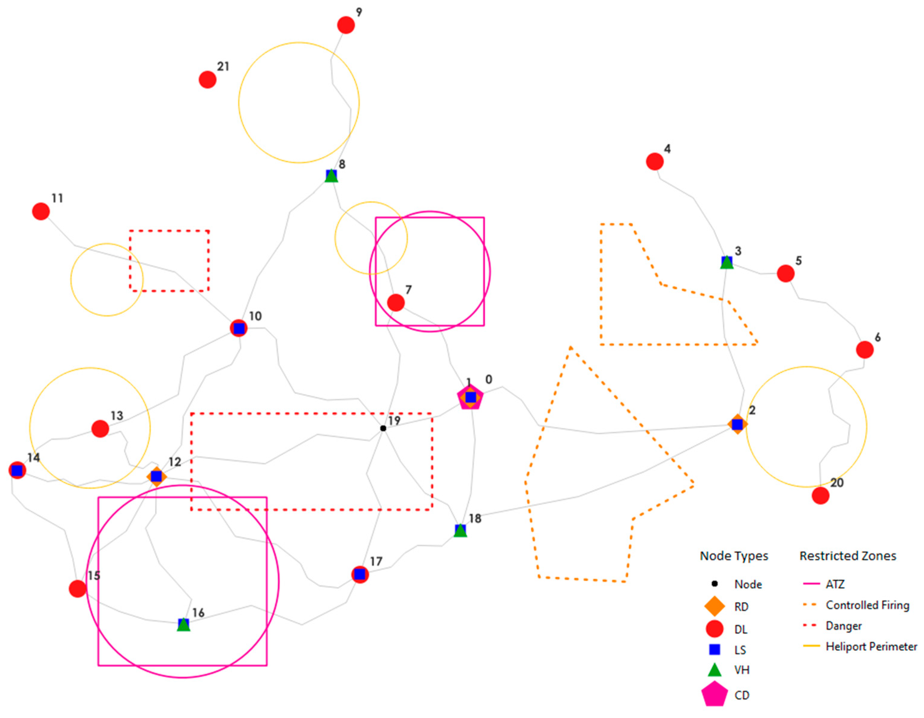
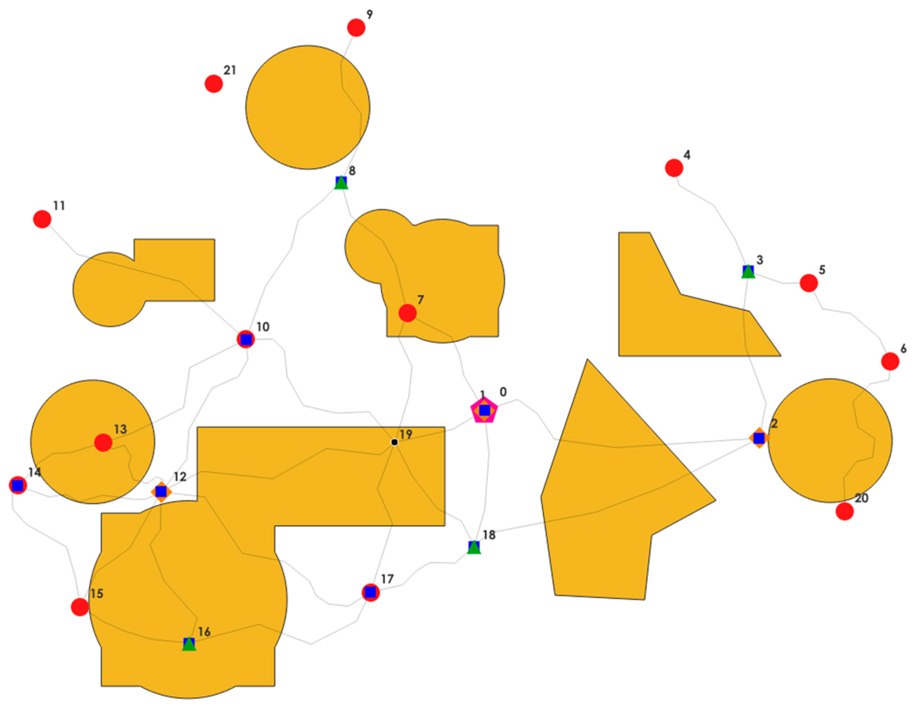
3.1. Base Network

3.1.1. Input Data

We devise a test CV network with all types of facilities (CD, RD, VH) and demand data, carrying benchmark characteristics, to perform a solid stress test on our algorithm.

The said network should offer certain features:

• The geographical size of the network should resemble that of a large city or the distances between neighboring cities.
• There must be dead-end edges, i.e., edges that are connected to a single node at one end (to resemble last-mile cases with limited connections).
• A node is not necessarily connected to all its closest ones (to emulate missing links).
• At some point, there must be a series of consecutive edges with a single node connection in between (to resemble possible stops along a single corridor).

As far as node types and delivery locations,

• There must be a CD and at least one RD (apart from the CD duplicate) away from it.
• There must be a few Virtual Hubs, distributed evenly throughout the network (not all Virtual Hubs will necessarily serve as allowed Launch Sites).
• There must be at least one Delivery Location outside the given CV network where only a UAV can be of service.

The following figures (Figure 10 and Figure 11) describe the case study network and its node types.

Certain specs for the CV and the UAV are selected. The specifications for the UAV resemble today’s advanced commercial UAVs and are naturally expected to improve in the future (see indicative enterprise-grade UAV specs at [54,55,56]).

• S^CV = 40 km/h, H^UAV = 120 m, S^UAV = 14.45 m/s
• S^UAV_asc = 4.25 m/s (tta = 28.2 s, for H^UAV = 120 m)
• S^UAV_des = 3.4 m/s (ttd = 35.3 s, for H^UAV = 120 m)
• R^UAV = 60 min (2400 s)

Service and transshipment times are assumed: st = 60 s (1 min), tc = 300 s (5 min). Input data regarding the base network are presented in Appendix A,

Table A1. Input CV network nodes’ basic information.

vi	x	y	vi	x	y
0	0.000	0.000	11	−35,652.764	15,493.993
1	0.000	0.000	12	−26,081.454	−6588.331
2	22,200.500	−2246.434	13	−30,736.252	−2595.080
3	21,339.640	11,254.890	14	−37,656.441	−6082.275
4	15,305.796	19,590.346	15	−32,594.951	−15,883.915
5	26,209.829	10,341.626	16	−23,794.972	−18,816.222
6	32,795.242	3940.702	17	−9184.639	−14,708.946
7	−6200.316	7871.878	18	−814.285	−10,979.538
8	−11,565.366	18,473.235	19	−7208.515	−2587.391
9	−10,318.214	30,943.160	20	29,121.346	−8156.159
10	−19,235.476	5729.837

and

Table A2. Actual length (L^CV_ij, m) of CV network links.

Lij

0

1

2

3

4

5

6

7

8

9

10

11

12

13

14

15

16

17

18

19

20

0

0

0

23,899

inf

inf

inf

inf

10,611

inf

inf

inf

inf

inf

inf

inf

inf

inf

inf

11,133

7752

inf

1

0

0

23,899

inf

inf

inf

inf

10,611

inf

inf

inf

inf

inf

inf

inf

inf

inf

inf

11,133

7752

inf

2

23,899

23,899

0

13,880

inf

inf

inf

inf

inf

inf

inf

inf

inf

inf

inf

inf

inf

inf

24,885

inf

inf

3

inf

inf

13,880

0

10,717

5038

inf

inf

inf

inf

inf

inf

inf

inf

inf

inf

inf

inf

inf

inf

inf

4

inf

inf

inf

10,717

0

inf

inf

inf

inf

inf

inf

inf

inf

inf

inf

inf

inf

inf

inf

inf

inf

5

inf

inf

inf

5038

inf

0

9870

inf

inf

inf

inf

inf

inf

inf

inf

inf

inf

inf

inf

inf

inf

6

inf

inf

inf

inf

inf

9870

0

inf

inf

inf

inf

inf

inf

inf

inf

inf

inf

inf

inf

inf

16,017

7

10,611

10,611

inf

inf

inf

inf

inf

0

12,358

inf

inf

inf

inf

inf

inf

inf

inf

inf

inf

11,020

inf

8

inf

inf

inf

inf

inf

inf

inf

12,358

0

13,583

15,285

inf

inf

inf

inf

inf

inf

inf

inf

inf

inf

9

inf

inf

inf

inf

inf

inf

inf

inf

13,583

0

inf

inf

inf

inf

inf

inf

inf

inf

inf

inf

inf

10

inf

inf

inf

inf

inf

inf

inf

inf

15,285

inf

0

19,703

15,115

15,413

inf

inf

inf

inf

inf

16,914

inf

11

inf

inf

inf

inf

inf

inf

inf

inf

inf

inf

19,703

0

inf

inf

inf

inf

inf

inf

inf

inf

inf

12

inf

inf

inf

inf

inf

inf

inf

inf

inf

inf

15,115

inf

0

8641

12,129

11,621

13,828

21,266

inf

20,338

inf

13

inf

inf

inf

inf

inf

inf

inf

inf

inf

inf

15,413

inf

8641

0

8088

inf

inf

inf

inf

inf

inf

14

inf

inf

inf

inf

inf

inf

inf

inf

inf

inf

inf

inf

12,129

8088

0

12,523

inf

inf

inf

inf

inf

15

inf

inf

inf

inf

inf

inf

inf

inf

inf

inf

inf

inf

11,621

inf

12,523

0

9433

inf

inf

inf

inf

16

inf

inf

inf

inf

inf

inf

inf

inf

inf

inf

inf

inf

13,828

inf

inf

9433

0

inf

inf

inf

inf

17

inf

inf

inf

inf

inf

inf

inf

inf

inf

inf

inf

inf

21,266

inf

inf

inf

inf

0

9629

12,908

inf

18

11,133

11,133

24,885

inf

inf

inf

inf

inf

inf

inf

inf

inf

inf

inf

inf

inf

inf

9629

0

10,852

inf

19

7752

7752

inf

inf

inf

inf

inf

11,020

inf

inf

16,914

inf

20,338

inf

inf

inf

inf

12,908

10,852

0

inf

20

inf

inf

inf

inf

inf

inf

16,017

inf

inf

inf

inf

inf

inf

inf

inf

inf

inf

inf

inf

inf

0

.

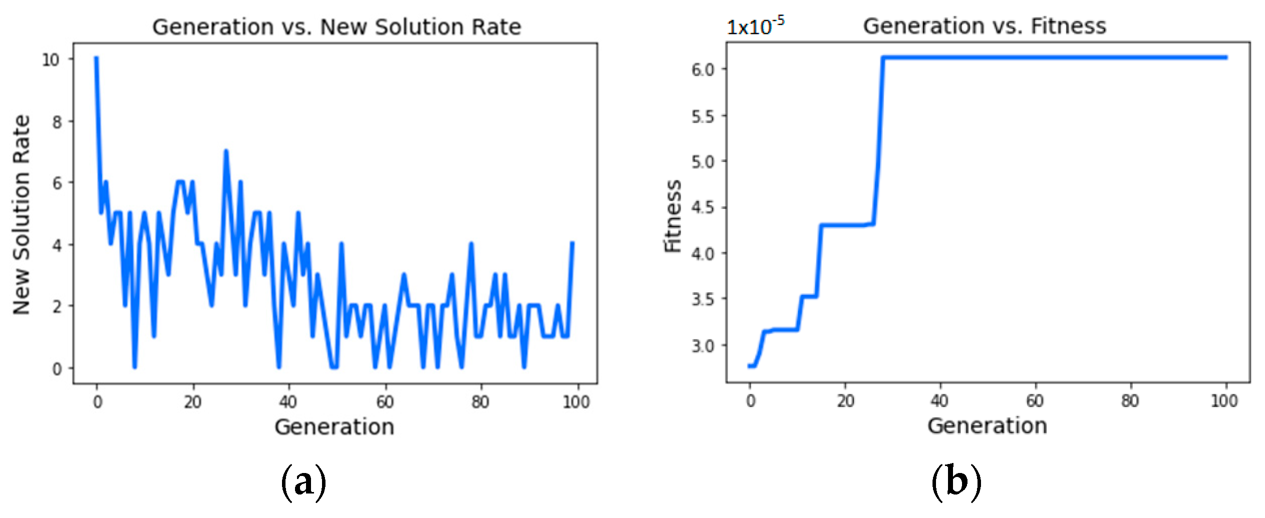
3.1.2. Application and Solution

A 60 min UAV range and a 40 km/h CV speed are selected, and RDs are placed at critical locations, based on the experience gained by previous experimentation.

The network is transformed into GIS format, and Restricted Zones (RZs) of various types and shapes are introduced. RZ sizes and shapes resemble common cases met in airspace no-fly zones (e.g., ATZs usually cover a range of 3000–8000 m around the airport). Such zones are commonly archived and updated in GIS databases; thus, we believe it makes sense to include such an approach in our framework. The RZs are shown in Figure 12 (as they would normally exist in relevant flight information maps), and Figure 13 depicts the final solid “obstacles” resulting from analysis in GIS.

DLs and potential LSs that fall within the RZs are removed from UAV operations. For each DL and its maximum potential LSs, optimal UAV paths around the RZs are calculated. The calculations are carried out through a flow direction algorithm [57], using D8 [58], Multiple Flow Direction (MFD) [59], or D-Infinity (DINF) [60] methods and accumulated cost surface and slope line [61]. An example of such analysis for our case study is shown in Figure 14, while Figure 15 includes all optimal paths created for initially reachable node pairs.

After establishing the shortest paths around the RZs, a further filter is applied, excluding paths that now exceed the UAV range, and the Service Nodes Pool is updated for each DL.

After running the algorithm and the optimization workflow, we have obtained the following results: GOT = 16,340.8 s, CVT = 16,340.8 s.

Figure 16 and Figure 17 below show the gene and solution evolution process through our nested GA algorithm.

The Service Nodes Pool, the assigned service node, and the final mode for each item are included in

Table 2. Potential Launch Sites and final Service Nodes Pool for items.

Item (k)	Node (dk)	Service Nodes Pool (SNk)					Assigned Service Node (lk)	Mode
1	4	4	0	2	3		0	UAV
2	5	5	2	3			2	UAV
3	6	6	2	3			2	UAV
4	7	7					7	CV
5	9	9	8				8	UAV
6	10	10	0	8	12	14	0	UAV
7	11	11	8	10	12	14	12	UAV
8	13	13					13	CV
9	14	14	10	12			12	UAV
10	15	15	12	14			12	UAV
11	17	17	0	18			0	UAV
12	20	20	2	3			2	UAV
13	21		8	10			8	UAV

.

Table 3. Routing information.

$T_{Ma}^v$	[‘0’, ‘2’, ‘7’, ‘8’, ‘12’, ‘13’]	Mandatory nodes with action
$T_M^v$	[‘0’, ‘1’, ‘2’, ‘7’, ‘8’, ‘12’, ‘13’]	Mandatory nodes
$\widehat{S_v^M}$	[‘0’, ‘2’, ‘13’, ‘12’, ‘8’, ‘7’, ‘1’]	Path of mandatory nodes
$\widehat{S_{\left(e\right)}^M}$	[(‘0’, ‘2’), (‘2’, ‘13’), (‘13’, ‘12’), (‘12’, ‘8’), (‘8’, ‘7’), (‘7’, ‘1’)]	Sequence of shell edges, through mandatory nodes
$\widehat{S_v}$	[[‘0’, ‘2’], [‘2’, ‘0’, ‘19’, ‘12’, ‘13’], [‘13’, ‘12’], [‘12’, ‘10’, ‘8’], [‘8’, ‘7’], [‘7’, ‘1’]]	Full path of nodes
$\widehat{S_{\left(e\right)}}$	[(‘0’, ‘2’), (‘2’, ‘0’), (‘0’, ‘19’), (‘19’, ‘12’), (‘12’, ‘13’), (‘13’, ‘12’), (‘12’, ‘10’), (‘10’, ‘8’), (‘8’, ‘7’), (‘7’, ‘1’)]	Full sequence of edges

describes how the CV routing is performed, while

Table 4. Path, actions, and time evolution (s).

ORDER	1 (CD)	2	3	4	5	6	7 (CD/RD)
MANDATORY NODE	0	2	13	12	8	7	1
PASS THROUGH		0, 9, 12		10
ACTION			Delivery			Delivery
	Launch	Launch		Launch	Launch		(end)
TAPP	0.0	2150.9	7787.7	8625.5	2736.0	15,325.8	16,340.8
${\mathit{c}\mathit{t}}_{\mathit{i}\mathit{j}}^{\mathit{M}}$	0.0	2150.9	5456.8	777.7	2736.0	1112.3	955.0
WI	0.0	180.0	60.0	180.0	2672.1	60.0	0.0
TDEP	0.0	2330.9	7847.7	8805.5	14,213.6	15,385.8	16,340.8
TRET	4530.3	5248.7	0.0	13,281.0	0.0	0.0	0.0
GOT (S)							16,340.8

shows the actions taken at each mandatory node and how time accumulates until the end of operations.

A graphical representation of the solution is shown in Figure 18.

We have recalculated the optimal solution, excluding the RZs, to compare the results. A GOT of 14,756.5 s has been obtained. In the presence of RZs, the GOT (16,340.8 s) was significantly higher (9.7%) and different assignment and routing options were selected. In Figure 19, the two solutions are depicted side by side in a similar simplistic manner for easier direct comparison.

4. Conclusions

We have developed a modular framework and a solution optimization methodology for integrated UAV and CV operations. Our entire platform offers flexibility in adaptation to infrastructure (links, nodes, types of facilities) and equipment (vehicle specs), network characteristics (missing links, dead-ends, butterfly routes), and the response to restricted airspace. Because of the need for safe UAV deployment sites and the high presence of restricted airspace zones in urban environments, the intended field of application is assumed to be the delivery of small packages in rural and under-connected areas, the execution of inter-city deliveries, and the expansion of a city’s original service range.

Each step, from inputs to final optimization, is part of a modular workflow that allows for preference-based solutions (e.g., constraints for certain locations, shortages in equipment, priority in deliveries, routing). Since not all nodes and edges of the physical network are necessarily visited, a shell network is created resulting from mandatory nodes and the shortest path total costs between them, deconstructing and simplifying the problem. Restricted Zones are considered for UAV flights, altering the traditional straight-line approach, and using obstacle routing instead. A GIS environment is used for spatial analysis and optimal path planning. We have developed a tailored nested GA method for obtaining optimal solutions in terms of mode assignment for each item and routing of the CV.

Our model was implemented in a case study with benchmark characteristics. Substantial gains in performance (total time of operations) can be achieved with wise infrastructure choices and improved equipment specifications. Experiments have shown the robustness of the formulation and general methodology from preliminary analysis to final solution optimization. The presence of Restricted Zones significantly alters the potential solutions and is worth considering for a more realistic approach. It is a modular workflow with an easy “front-end” and a solid mathematical background that can be practically used for decision-making purposes at a strategic level and is open to future adaptations.

The entire model and solution methodology are practical tools for decision making and strategic planning, but we offer some specific novelties. For example, our variable Launch Site types for LARO, the tailored Assignment and Routing Optimization nested GA, the consideration of airspace restrictions of any shape and size, the inclusion of GIS tools in the process, the modularity of our platform, and, most importantly, the inclusion of all the above in a single, comprehensive, and holistic approach could be highlighted. In terms of the transport system setup, further research could be directed toward including more CVs instead of one, considering altitude and terrain specifics and the stochastic nature of travel times both for the CVs and UAVs.

References

1. European Commission. Emission Performance Standards for New Passenger Cars and for New Light Commercial Vehicles; European Commission: Brussels, Belgium, 2017. [Google Scholar]
2. Witkamp, B.; van Gijlswijk, R.; Bolech, M.; Coosemans, T.; Hooftman, N.S. The Transition to a Zero Emission Vehicles Fleet for Cars in the EU by 2050: Pathways and Impacts: An Evaluation of Forecasts and Backcasting the COP21 Commitments; European Alternative Fuels Observatory: Brussels, Belgium, 2017. [Google Scholar]
3. Davies, C. The Carbon Cost of Home Delivery and How to Avoid It. Horizon: The EU Research & Innovation Magazine. 17 February 2020. Available online: https://ec.europa.eu/research-and-innovation/en/horizon-magazine/carbon-cost-home-delivery-and-how-avoid-it (accessed on 14 March 2023).
4. ITF. Ready for Take Off? Integrating Drones into the Transport System; OECD Publishing: Paris, France, 2021. [Google Scholar]
5. Roland Berger Gmbh. Cargo Drones: The Future of Parcel Delivery (USD 5.5 Billion Market). Roland Berger Gmbh, 19 February 2020. Available online: https://www.rolandberger.com/en/Point-of-View/Cargo-drones-The-future-of-parcel-delivery.html (accessed on 10 September 2022).
6. McKinsey & Company. Up in the Air: How Do Consumers View Advanced Air Mobility? McKinsey Global Publishing, May 2021. Available online: https://www.mckinsey.com/industries/aerospace-and-defense/our-insights/up-in-the-air-how-do-consumers-view-advanced-air-mobility (accessed on 1 June 2021).
7. Murray, C.C.; Chu, A.G. The flying sidekick traveling salesman problem: Optimization of drone-assisted parcel delivery. Transp. Res. Part C Emerg. Technol. 2015, 54, 86–109. [Google Scholar] [CrossRef]
8. Ferrandez, S.M.; Harbison, T.; Weber, T.; Sturges, R.; Rich, R. Optimization of a Truck-drone in Tandem Delivery Network Using K-means and Genetic Algorithm Sergio. J. Ind. Eng. Manag. 2016, 9, 374–388. [Google Scholar]
9. MacQueen, J.B. Some Methods for Classification and Analysis of Multivariate Observations. Berkeley Symp. Math. Stat. Probab. 1967, 5, 281–297. [Google Scholar]
10. Moshref-Javadi, M.; Lee, S.; Winkenbach, M. Design and evaluation of a multi-trip delivery model with truck and drones. Transp. Res. E Logist. Transp. Rev. 2020, 136, 101887. [Google Scholar] [CrossRef]
11. Salama, M.R.; Srinivas, S. Collaborative truck multi-drone routing and scheduling problem: Package delivery with flexible launch and recovery sites. Transp. Res. E Logist. Transp. Rev. 2022, 164, 102788. [Google Scholar] [CrossRef]
12. Marinelli, M.; Caggiani, L.; Ottomanelli, M.; Dell, M. En route truck–drone parcel delivery for optimal vehicle routing strategies. IET Intell. Transp. Syst. 2017, 12, 253–261. [Google Scholar] [CrossRef]
13. Chang, Y.S.; Lee, H.J. Optimal delivery routing with wider drone-delivery areas along a shorter truck-route. Expert Syst. Appl. 2018, 104, 307–317. [Google Scholar] [CrossRef]
14. Agatz, N.; Bouman, P.; Schmidt, M. Optimization Approaches for the Traveling Salesman Problem with Drone. Transp. Sci. 2018, 52, 965–981. [Google Scholar] [CrossRef]
15. Gonzalez-R, P.L.; Canca, D.; Andrade-Pineda, J.L.; Calle, M.; Leon-Blanco, J.M. Truck-drone team logistics: A heuristic approach to multi-drop route planning. Transp. Res. C Emerg. Technol. 2020, 114, 657–680. [Google Scholar] [CrossRef]
16. Jeong, H.Y.; Song, B.D.; Lee, S. Truck-drone hybrid delivery routing: Payload-energy dependency and No-Fly zones. Int. J. Prod. Econ. 2019, 214, 220–233. [Google Scholar] [CrossRef]
17. Zhou, H.; Qin, H.; Cheng, C.; Rousseau, L.-M. An exact algorithm for the two-echelon vehicle routing problem with drones. Transp. Res. B Methodol. 2023, 168, 124–150. [Google Scholar] [CrossRef]
18. Momeni, M.; Al-E-Hashem, S.M.J.M.; Heidari, A. A new truck-drone routing problem for parcel delivery by considering energy consumption and altitude. Ann. Oper. Res. 2023, 1–47. [Google Scholar] [CrossRef] [PubMed]
19. Li, H.; Chen, J.; Wang, F.; Zhao, Y. Truck and drone routing problem with synchronization on arcs. Nav. Res. Logist. 2022, 69, 884–901. [Google Scholar] [CrossRef]
20. Leon-Blanco, J.M.; Gonzalez-R, P.; Andrade-Pineda, J.L.; Canca, D.; Calle, M. A multi-agent approach to the truck multi-drone routing problem. Expert Syst. Appl. 2022, 195, 116604. [Google Scholar] [CrossRef]
21. Li, H.; Wang, F. Branch-price-and-cut for the truck–drone routing problem with time windows. Nav. Res. Logist. 2022, 70, 184–204. [Google Scholar] [CrossRef]
22. Boysen, N.; Briskorn, D.; Fedtke, S.; Schwerdfeger, S. Drone delivery from trucks: Drone scheduling for given truck routes. Networks 2018, 72, 506–527. [Google Scholar] [CrossRef]
23. Macrina, G.; Pugliese, L.D.P.; Guerriero, F.; Laporte, G. Drone-aided routing: A literature review. Transp. Res. Part C Emerg. Technol. 2020, 120, 102762. [Google Scholar] [CrossRef]
24. Rardin, R.L. Optimization in Operations Research, 2nd ed.; Pearson Higher Education, Inc.: Hoboken, NJ, USA, 2015. [Google Scholar]
25. Dantzig, G.; Fulkerson, R.; Johnson, S. Solution of a large-scale Traveling Salesman Problem. Oper. Res. 1954, 2, 393–410. [Google Scholar] [CrossRef]
26. Bellman, R. Dynamic Programming Treatment of the Travelling Salesman Problem. J. ACM 1962, 9, 61–63. [Google Scholar] [CrossRef]
27. Little, J.D.; Murty, K.G.; Sweeney, D.W.; Karel, C. An algorithm for the traveling salesman problem. Oper. Res. 1963, 11, 972–989. [Google Scholar] [CrossRef]
28. Garey, M.R.; Johnson, D.S. Computers and Intractability: A Guide to NP-Completeness; WH Freeman: New York, NY, USA, 1979. [Google Scholar]
29. Applegate, D.; Bixby, R.; Chvátal, V.; Cook, W. Finding Cuts in the TSP (A Preliminary Report); Center for Discrete Mathematics & Theoretical Computer Science: Piscataway, NJ, USA, 1995. [Google Scholar]
30. Applegate, D.; Bixby, R.; Chvátal, V.; Cook, W. The Traveling Salesman Problem. In Combinatorial Optimization: Theory and Algorithms, 4th ed.; Springer: Berlin/Heidelberg, Germany, 2008; Volume 21, pp. 527–562. [Google Scholar]
31. Held, M.; Karp, R.M. A dynamic programming approach to sequencing problems. J. Soc. Ind. Appl. Math. 1962, 10, 196–210. [Google Scholar] [CrossRef]
32. Kirkpatrick, S.; Gelatt, C.D.; Vecchi, M.P. Optimization by Simulated Annealing. Science 1983, 220, 671–680. [Google Scholar] [CrossRef] [PubMed]
33. Holland, J.H. Adaptation in Natural and Artificial Systems; Arbor, A., Ed.; University of Michigan Press: Ann Arbor, MI, USA, 1975. [Google Scholar]
34. Glover, F. Future paths for integer programming and links to artificial intelligence. Comput. Oper. Res. 1986, 13, 533–549. [Google Scholar] [CrossRef]
35. Glover, F. Tabu Search—Part I. ORSA J. Comput. 1989, 1, 190–206. [Google Scholar] [CrossRef]
36. Glover, F. Search—Part II. ORSA J. Comput. 1990, 2, 4–32. [Google Scholar] [CrossRef]
37. Dijkstra, E.W. A note on two problems in connexion with graphs. Numer. Math. 1959, 1, 269–271. [Google Scholar] [CrossRef]
38. Hart, P.E.; Nilsson, N.J.; Raphael, B. A Formal Basis for the Heuristic Determination of Minimum Cost Paths. IEEE Trans. Syst. Sci. Cybern. 1968, 4, 100–107. [Google Scholar] [CrossRef]
39. Korf, R.E. Depth-first iterative-deepening: An optimal admissible tree search. Artif. Intell. 1985, 27, 97–109. [Google Scholar] [CrossRef]
40. Koenig, S.; Likhachev, M.; Furcy, D. Lifelong Planning A∗. Artif. Intell. 2004, 155, 93–136. [Google Scholar] [CrossRef]
41. ICAO. Annex 11 to the Convention on International Civil Aviation—Air Traffic Services; International Civil Aviation Organization: Montreal, QC, Canada, 2018. [Google Scholar]
42. EASA. Easy Access Rules for Unmanned Aircraft Systems; European Union: Brussels, Belgium, 2022. [Google Scholar]
43. ICAO. Annex 2 to the Convention on Civil Aviation—Rules of the Air, 10th ed.; International Civil Aviation Organization: Montreal, QC, Canada, 2005. [Google Scholar]
44. FAA. Chapter 15—Airspace. In Pilots Handbook of Aeronautical Knowledge; Federal Aviation Administration: Washington, DC, USA, 2016. [Google Scholar]
45. FAA. Aeronautical Information Publication (AIP); Federal Aviation Administration: Washington, DC, USA, 2022. [Google Scholar]
46. HCAA. Drone Aware—GR (DAGR). Hellenic CAA. 2023. Available online: https://dagr.hasp.gov.gr/ (accessed on 1 June 2023).
47. Lumelsky, V.; Stepanov, A.A. Path-planning strategies for a point mobile automaton moving amidst unknown obstacles of arbitrary shape. Algorithmica 1987, 2, 403–430. [Google Scholar] [CrossRef]
48. Kamon, I.; Rimon, E.; Rivlin, E. TangentBug: A Range-Sensor-Based Navigation Algorithm. Int. J. Robot. Res. 1998, 17, 934–953. [Google Scholar] [CrossRef]
49. Kamon, I.; Rivlin, E.; Rimon, E. A New Range-Sensor Based Globally Convergent Navigation Algorithm for Mobile Robots. In Proceedings of the IEEE International Conference on Robotics and Automation, Minneapolis, MN, USA, 22–28 April 1996. [Google Scholar]
50. Rashid, A.T.; Ali, A.A.; Frasca, M.; Fortuna, L. Path Planning and Obstacle Avoidance Based on Shortest Distance Algorithm. In Proceedings of the Second Al-Sadiq International Conference on Multidisciplinary in IT and Communication Science and Applications, Baghdad, Iraq, 22–23 November 2017. [Google Scholar]
51. Khatib, O. Real-time obstacle avoidance for manipulators and mobile robots. Int. J. Robot. Res. 1986, 5, 90–98. [Google Scholar] [CrossRef]
52. Iliopoulou, C.; Kepaptsoglou, K.; Karlaftis, M.G. Route Planning for a Sea Plane Service: The Case of the Greek Islands. Comput. Oper. 2015, 59, 66–77. [Google Scholar] [CrossRef]
53. Lenstra, J.K.; Kan, A.H.G.R. Complexity of vehicle routing and scheduling problems. Networks 1981, 11, 221–227. [Google Scholar] [CrossRef]
54. DJI. DJI Matrice 300 RTK Specs. 2023. Available online: https://enterprise.dji.com/matrice-300/specs (accessed on 15 August 2023).
55. Flying Basket. FB3—The Most Compact Drone in the World Able to Carry 100 kg. 2023. Available online: https://flyingbasket.com/fb3 (accessed on 15 August 2023).
56. Matternet. Matternet—M2. 2023. Available online: https://www.engineeringforchange.org/solutions/product/matternet-m2/ (accessed on 15 August 2023).
57. ESRI. “Flow Direction”. 2023. Available online: https://desktop.arcgis.com/en/arcmap/latest/tools/spatial-analyst-toolbox/flow-direction.htm (accessed on 1 August 2023).
58. Jenson, S.K.; Domingue, J.O. Extracting Topographic Structure from Digital Elevation Data for Geographic Information System Analysis. Photogramm. Eng. Remote Sens. 1988, 54, 1593–1600. [Google Scholar]
59. Qin, C.; Zhu, A.X.; Pei, T.; Li, B.; Zhou, C.; Yang, L. N adaptive approach to selecting a flow partition exponent for a multiple flow direction algorithm. Int. J. Geogr. Inf. Sci. 2007, 21, 443–458. [Google Scholar] [CrossRef]
60. Tarboton, D.G. A new method for the determination of flow directions and upslope areas in grid digital elevation models. Water Resour. Res. 1997, 33, 309–319. [Google Scholar] [CrossRef]
61. Douglas, D.H. Least-cost Path in GIS Using an Accumulated Cost Surface and Slopelines. Cartogr. Int. J. Geogr. Inf. Geovisualization 1994, 31, 37–51. [Google Scholar] [CrossRef]
Figure 1. Symbols and notations for general concept.
Vehicles 05 00058 g001
Figure 2. Setup Example 1—Infrastructure, demand, and UAV range: (a) infrastructure and demand; (b) UAV range (indicative, from one of the launch sites).
Vehicles 05 00058 g002
Figure 3. Setup Example 1—Possible assignment and routing solutions: (a) solution 1: deliveries with truck and with UAVs from Remote Depot; (b) solution 2: deliveries only with UAVs from Remote Depot.
Vehicles 05 00058 g003
Figure 4. General methodology workflow.
Vehicles 05 00058 g004
Figure 5. Venn diagram; schematic representation of node sets.
Vehicles 05 00058 g005
Figure 6. Simplified illustration of VTOL-type flight and associated variables.
Vehicles 05 00058 g006
Figure 7. Two-level identification process of UAV feasible connections between LSs and DLs.
Vehicles 05 00058 g007
Figure 8. Example of assignment GA chromosomes and offspring through single-point crossover.
Vehicles 05 00058 g008
Figure 9. Example of routing GA chromosomes and offspring.
Vehicles 05 00058 g009
Figure 10. (a) Original input CV network, with node numbers and road links, (b) graph representation, with nodes and edges.
Vehicles 05 00058 g010
Figure 11. CV network and node types.
Vehicles 05 00058 g011
Figure 12. Illustration of introduced Restricted Zones.
Vehicles 05 00058 g012
Figure 13. Dissolving Restricted Zones into integrated no-fly areas. Orange shapes indicate final RZs.
Vehicles 05 00058 g013
Figure 14. Example of optimal paths between a DL and LSs: (a) LSs in maximum UAV range of DL (UAV range from Node 10, indicated by red circle); (b) optimal paths for initially feasible LSs (paths shown as green lines around purple RZs).
Vehicles 05 00058 g014
Figure 15. All UAV optimal paths between DLs and potential LSs within maximum UAV range. Lines around purple RZs show respective paths between node pairs.
Vehicles 05 00058 g015
Figure 16. Nested GA mode assignment solutions (outer GA genes).
Vehicles 05 00058 g016
Figure 17. Nested GA results evolution: (a) generation vs. new solution rate; (b) generation vs. fitness.
Vehicles 05 00058 g017
Figure 18. GIS-based illustration of the best solution under constrained airspace.
Vehicles 05 00058 g018
Figure 19. Simplified illustration of assignment and routing solutions: (a) without RZs; (b) with RZs.
Vehicles 05 00058 g019