Abstract
Reducing costs and time spent in experiments in the early development stages of vehicular technology such as off-road and agricultural semi-autonomous robots could help progress in this research area. In particular, evaluating path tracking strategies in the semi-autonomous operation of robots becomes challenging because of hardware costs, the time required for preparation and tests, and constraints associated with external aspects such as meteorological or weather conditions or limited space in research laboratories. This paper proposes a methodology for the real-time hardware-in-the-loop emulation of path tracking strategies in low-cost agricultural robots. This methodology enables the real-time validation of path tracking strategies before their implementation on the robot. To validate this, we propose implementing a path tracking strategy using only the information of motor’s angular speed and robot yaw velocity obtained from encoders and a low-cost inertial measurement unit (IMU), respectively. This paper provides a simulation with MATLAB/Simulink, hardware-in-the-loop with Qube-servo (Quanser), and experimental results with an Agribot platform to confirm its validity.
1. Introduction
Zero hunger, affordable and clean energy, innovation, infrastructure modernization, and industry appear as important priorities according to the Sustainable Development Goals (SDGs) of the United Nations [1]. Following these objectives, the modernization of farming by introducing clean and affordable energy and machinery can be a huge contribution to humanity [2]. Thus, developing sustainable semi-autonomous robots and off-road electric or hybrid vehicles could help to eradicate poverty and hunger and prevent climate change. Some hybrid drive technology considers using non-electrical elements including hydraulic or air pressure actuators and mechanical energy storage [3]. As mentioned in [2], hybrid systems with biomass and hydrogen technologies could also be useful for implementing sustainable machinery.
Agricultural robots (Agribots) can be seen as unmanned ground vehicles (UGVs) that must accomplish specific tasks in outdoor (fields) or indoor (greenhouses) scenarios. It is necessary to highlight that when used in fields, these vehicles require better stability and precision to adapt their behaviour to abrupt changes on the ground, ambient conditions, and driving modes. Likewise, using electric vehicles for these implementations requires analyzing recharging modes and adopting control methods that consider previously mentioned changes [4], and make them smarter. As a particular case, electric agricultural tractors represent zero-emission ecological solutions. These advances are led by countries such as Germany and Italy [5]. According to a Custom Market Insights (CMI) report, in 2021 the global electric tractor market size was estimated at USD 118 million, and it is expected to reach 250 million by 2030.
Current research and development are focused, principally, on autonomous operation, motion prediction, and correction of trajectories [6,7,8,9]. Likewise, there are works related to vehicle route planning [10], optimization of routes, and vehicle routing [11]. Here, it is important to mention that the research oriented on UGV navigation for indoor and outdoor applications [12], Ref. [13] requires the integration of multiple sensors [14,15,16]. On the other hand, there are road and off-road applications focused on integrating hybrid systems which can improve the favourability and the energetic vehicle performance using clean sources [17,18]. A good example of a solar PV electric vehicle charging ecosystem is studied in [19]; this research shows the advantages and limitations related to the production of electricity by a photovoltaic carport for recharging electric vehicles (EVs). Considering the stability of UGVs and autonomous mobile robots (AMRs), it is possible to find works focused on dynamic analysis and non-linear control to prevent problems such as rollover in trajectory tracking and path following [20], and the presence of lateral and longitudinal slips of wheels [21]. Recent works consider the use of model predictive control (MPC), dynamic adaptive control [22], disturbance rejection methods [23], backstepping, adaptive neural networks, adaptive fuzzy control [24,25], sliding mode control [26], and observers to mitigate the effect of non-linear characteristics and perturbations [21].
Independently of the application, modelling such robots and vehicles is one of the first steps in their development and control. This process is based on considerations for describing the kinematic and dynamic behaviour of the system [27,28]. It is possible to make these models using parameters such as the type and disposition of wheels and the shape of the vehicle’s frame. This information can determine posture, restrictions, and degree of mobility and manoeuvrability (steerability). After estimating the model parameters, they can be used in feedback loops to design and implement control strategies such as path tracking and energy estimation and management [29,30,31]. Thus, kinematic and dynamic models are fundamental for developing electric off-road vehicles and Agribots [32].
Considering a semi-autonomous outdoor operation of Agribots, as a particular case of UGVs, evaluating path tracking strategies could be challenging, time-consuming, and expensive. These difficulties can be accentuated in the early stages of development, where the incertitude of measurements, power electronics, and program behaviour is high. In some cases, this evaluation can be complicated by external factors such as meteorological conditions and space limitations in academic research laboratories. Simulation can also be time-consuming and, in some cases, limited by the accuracy and details of models. Under this perspective, the hardware-in-the-loop (HIL) emulation could be an intermediate solution to reduce costs and burdens and make it possible to evaluate control strategies in the early stages of Agribots development [33]. In the Industry 4.0 concept, as proposed in [34], digital twins technology, which includes physical and digital parts, can facilitate the test of AMRs under different operating environments. Digital twins and HIL technologies could help to accelerate the implementation of smarter AMRs.
In this paper, we address the problem of preliminary validation of path tracking strategies in Agribots by proposing a methodology for real-time hardware-in-the-loop emulation using a Qube servo from Quanser (https://www.quanser.com) and MATLAB/Simulink. The main contributions of this work are the proposition of a methodology of real-time hardware-in-the-loop emulation itself that allows the preliminary evaluation of path tracking strategies, saving time and infrastructure costs, as well as the proposition and experimental validation of a low complexity kinematic-based strategy that allows path tracking implementation with acceptable path offset in outdoor scenarios and using low-cost hardware. More specifically, this paper details hardware and software implementation for emulation and experimental evaluation using a real Agribot platform with a differential drive and dc motors controlled by an embedded microcomputer programmed using Python. We propose implementing the path tracking strategy based only on the kinematic model and the information on the motors’ angular speed and the robot’s yaw velocity. These pieces of information are obtained from two encoders, one for each motor and a low-cost inertial measurement unit (IMU), respectively.
The paper is organized to present, in Section 2, the theoretical background describing the mathematical formulation of the kinematics model, the speed controllers, and the path tracking strategies; in Section 3, the proposed methodology for real-time hardware-in-the-loop emulation; in Section 4, the experimental results of the hardware-in-the-loop and the experimental tests with the Agribot platform; and in Section 5, a discussion of the results obtained in the previous section. The paper ends with concluding remarks in Section 6.
2. Theoretical Background and System Modelling
This section introduces the base knowledge of kinematics modelling of the agricultural robot system under study and the considerations for implementing angular speed control and path tracking.
2.1. Kinematic Analysis
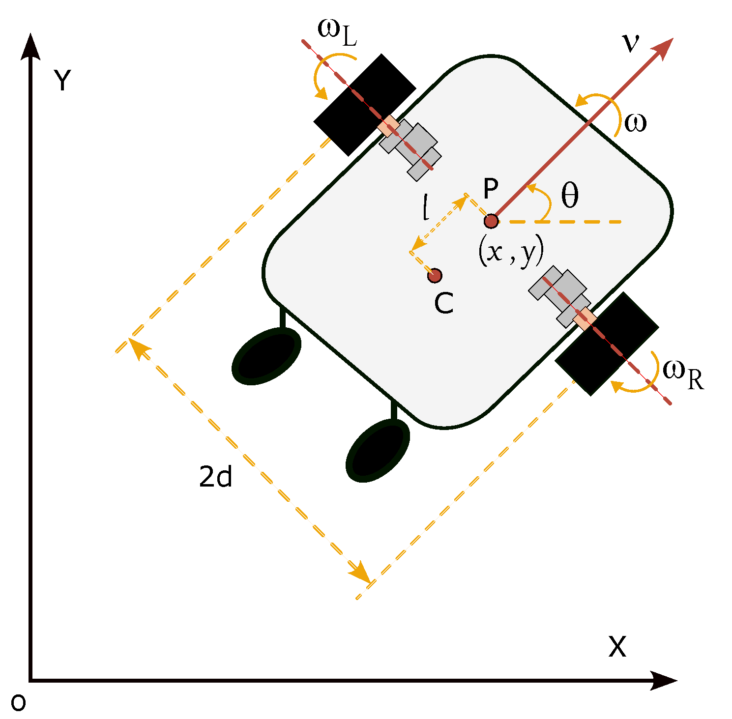
A wheeled vehicle, whatever its design and configuration, can be modelled in terms of one local reference frame and taking into account its main characteristics and wheels configuration. Figure 1 shows the first approach of the description of a vehicle across the global reference frame due to the X and Y axes, a local reference frame (x and y-axis), and an inertial point (P).

Figure 1.
General scheme of posture for a vehicle [27].
Modelling the motion in the global reference frame, from the origin (O) to P as the vector (), it is possible to define the vehicle’s posture (p), considering the local reference frame, in terms of the x, y, and variables [27].
Note that is the orientation angle, in [rad], between the local and global reference frames. In the case under study, the vehicle in Figure 1 corresponds to a standard model with two front-fixed wheels with independent traction and two rear-type castor-free wheels. There, point C represents the center of mass, d is the distance between P and the wheels across the y-axis, and l is the distance between P and C.
Once the orientation, , and the movement, and , of the vehicle are referenced to the local reference frame, it is possible to define the linear velocity of the vehicle as:
where and are the velocities, in [m/s], across each axis, and they are defined as:
Taking into account the trigonometrical relations, it is easy to find that the orientation of the vehicle can be defined as
Likewise, it is possible to define the equations of angular velocity, in [rad/s], for each wheel as:
where r [m] is the radius of wheels, R is the speed reduction ratio, [rad/s] is the angular yaw velocity of the vehicle across the global reference frame () view from P, which can be defined as:
Likewise, it is possible to define v in terms of and .
Now, substituting (9) in (3) and (4) the equations of and can be expressed in terms of the angular velocity of the wheels. Then, the equations related to the inverse kinematics of the vehicle are:
One can use these equations to implement feedback control considering perfect conditions on the ground and on the robot’s behaviour. However, in realistic scenarios, information from additional sensors must be employed to implement closed-loop position control with acceptable performance.
2.2. DC Motors Modelling and Angular Speed Control
The dynamics of the dc motor can be described by using the following second-order formulation
that allow the following transfer function to be obtained
where is the angular speed in [rad/s], is the voltage applied by the dc–dc converter in [volts], is the inertia constant in [kg ], is the friction constant in [Nm/(rad/s)], and are the inductance and resistance of the motor in [H] and [Ohms], respectively, is torque constant in [Nm/A], and is the voltage constant in [volts/(rad/s)].
This formulation can be adapted to a first-order approximation by neglecting the effects of the inductance and the friction constant and considering the possible transport delays (L) present in the system.
In an operational context, which can include dc–dc converters, measurement systems, data acquisition, and electronic control units, K, , and L can be obtained by means of open-loop tests. These results can be used to confirm the voltage constant , and to obtain , if the resistance and the voltage and torque constants are known. Typically, manufacturers provide the information of these parameters, and .
The first-order approximation with the transport delay of (15) can be employed to obtain the gains of the classic PID controllers using Ziegler–Nichols [35] or Cohen–Coon [36] empiric rules. The first one is well adapted and recommended for systems with , and the second when ; otherwise, the dead-time rule is needed. When L becomes significant compared to , i.e., , the system becomes more challenging to control, and PI is preferred over PID to keep stability. Using the Ziegler–Nichols rule, the PI gains can be obtained using,
On the other hand, using the Cohen–Coon rule, one can estimate
Likewise, using the dead-time tuning rule it is possible to calculate,
where determines the stability margin, typically between 1 and 4. A high value of allows a reduction of the overshoot but slows the response.
2.3. Path Tracking Strategy
We initially consider the path tracking strategy proposed in [37], with control parameters , , and tuned to reduce position and orientation angle errors. In this strategy, the actual robot orientation (yaw) angle , and the desired angle between the actual and the final position, , are used to define the angular velocity correction, , using
and, the linear velocity correction, , can be defined by,
using these angular and linear velocity correction terms, and , it is possible to define the angular speed to be imposed on each motor, and , as follows
This method can be easily implemented in digital processors using the function; however, the interpretation of the result of in (23) must be correctly handled when the result of the angle is higher than . A misinterpretation of angle correction results in abnormal or chaotic behaviour of the robot.
To correct this problem, we propose to obtain the signal for the angular velocity correction, , by using
with,
Notice that the system, for angle control purposes, can be approximated to a transfer function with an integral term () and a time constant (), as follows
where is the equivalent time constant of the angular speed controller of wheels; the system dynamics includes a delay L, as described in (15). Under this assumption, using a simple proportional controller with gain , as proposed in (27), the closed-loop transfer function will produce zero steady-state errors. To keep stability, it is recommended to set the gain to obtain enough phase (and delay) margin to tolerate the delays mentioned in (15). Normally, this gain will produce a response with a small overshoot or over-damped.
The control signal for the linear velocity correction, , is generated similarly to (24), and it can be obtained by using
Notice that the linear velocity correction by using proportional gains in (24) and (33) produces a non-zero steady-state error. Thus, the robot keeps a distance from its actual position to the next point of the trajectory. This prevents the robot from turning in circles when it surpasses the destination position. The term in (33) produces a reduction of linear velocity () when a high angle correction is needed, contributing to the stable behaviour of the robot. In that case, and similarly to (32), the system can be approximated to a first-order transfer function as follows
The reference of angular speed, and , is generated using (25) and (26) from the references of angular and linear velocities, obtained by (27) and (33).
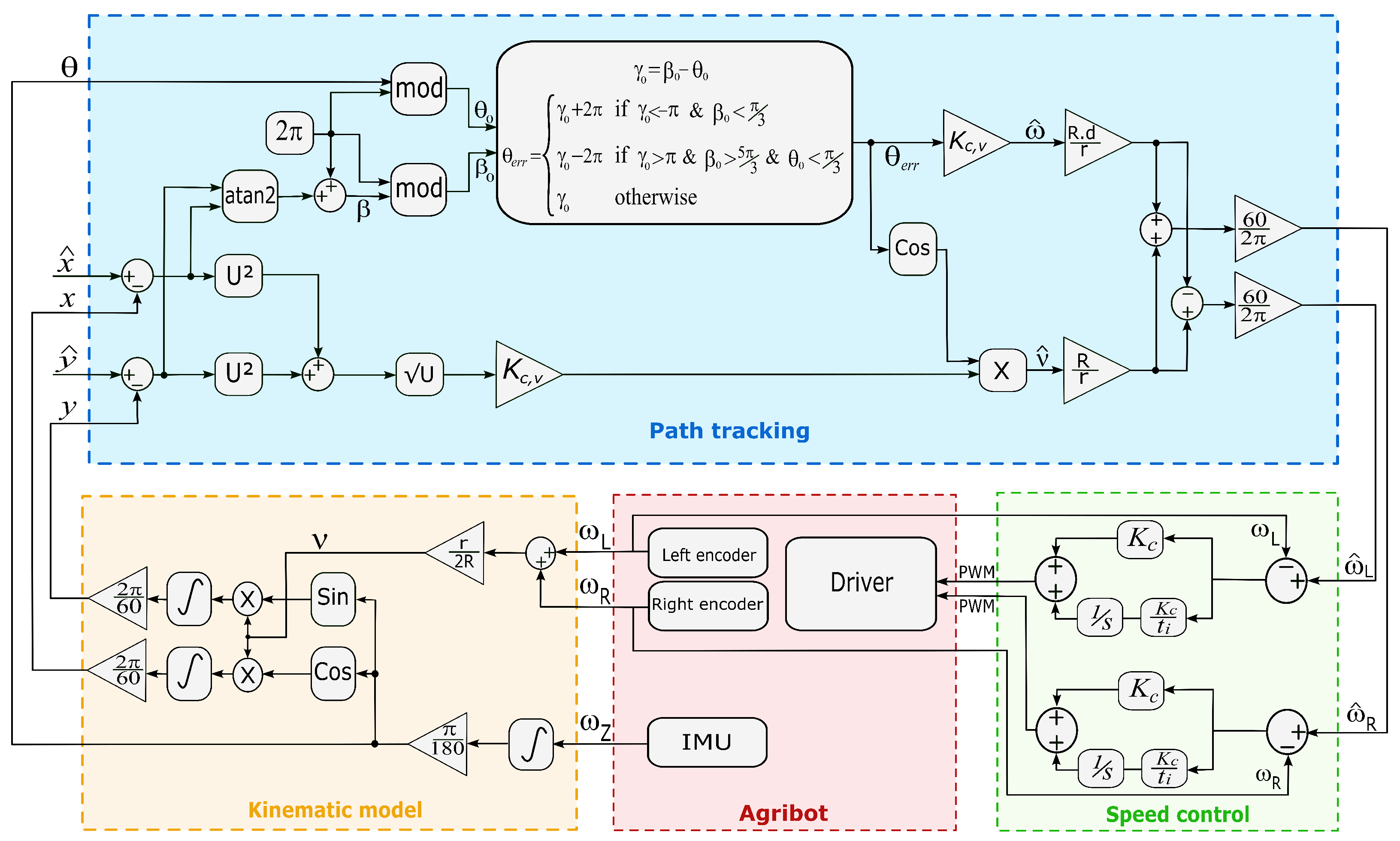
Figure 2 presents a simplified block diagram of the proposed path tracking strategy and control loops.

Figure 2.
Simplified diagram of the proposed path tracking strategy and control loops.
2.4. Localization of the Agribot
Localization of the Agribot can be achieved using different approaches [38]; in this study, the posture of the robot (1) for emulation purposes can be obtained by the formulation of the inverse kinematics model formulation of x, y, and , which are defined, respectively, by (10), (11), and (5).
For experiments with the Agribot, we employ an inertial measurement unit (IMU) from WitMotion (https://witmotion-sensor.com/) to obtain the yaw angular velocity of the robot, which allows us to compute the robot’s orientation (yaw) angle by integration. We also use two encoders, from USDigital (https://www.usdigital.com/), to obtain the angular velocity of each wheel, and ; from this information and the orientation, we can establish the actual position x, y, of the robot using the inverse kinematics model, (10) and (11). Thus, we can close the loop and control the robot’s position.
3. Real-Time Emulation of Agribot
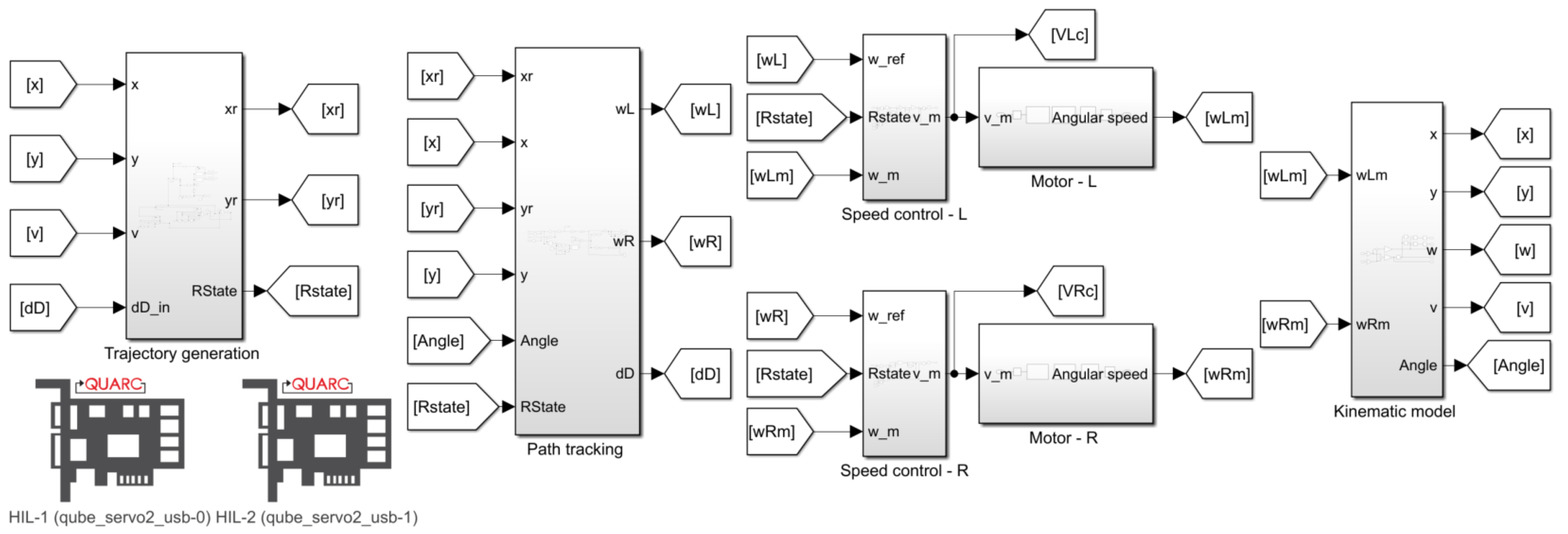
The proposed HIL real-time emulation methodology is depicted in Figure 3. In this approach, the kinematic model and controllers are implemented in MATLAB/Simulink (R2021a), and the motors of each wheel of the robot are emulated using two Qube servo 2 and the Quanser Real-Time Control (QUARC-V.4.1.363, 2021 SP1), toolbox from Quanser (https://www.quanser.com). The idea behind this HIL model is to enable the preliminary tests of path tracking strategies under conditions near a real scenario of robot operation.

Figure 3.
MATLAB/Simulink diagram of the implemented model for real-time emulation using Qube servo 2 from Quanser (https://www.quanser.com).
3.1. System Description and Characterisation
Table 1 summarizes some characteristics of this experimental platform, and Figure 4 presents a real view and depicts the main functional blocks of the Agribot. For emulation purposes, we use the characteristics of the motor of the Qube servo 2, volts/(rad/s), Ohm, mH, and kgm. These parameters give a time constant s, and a static gain rad/s/volts.

Table 1.
Components and specifications of the Agribot [39].

Figure 4.
Real view and simplified diagram of the hardware configuration of the Agribot.
For experimental validation, we performed open-loop tests to obtain the parameters of each motor–gearbox–wheel subsystem of the Agribot. These tests allowed the following parameters to be obtained for the approximation of the first-order transfer function with transport delay described by (15)
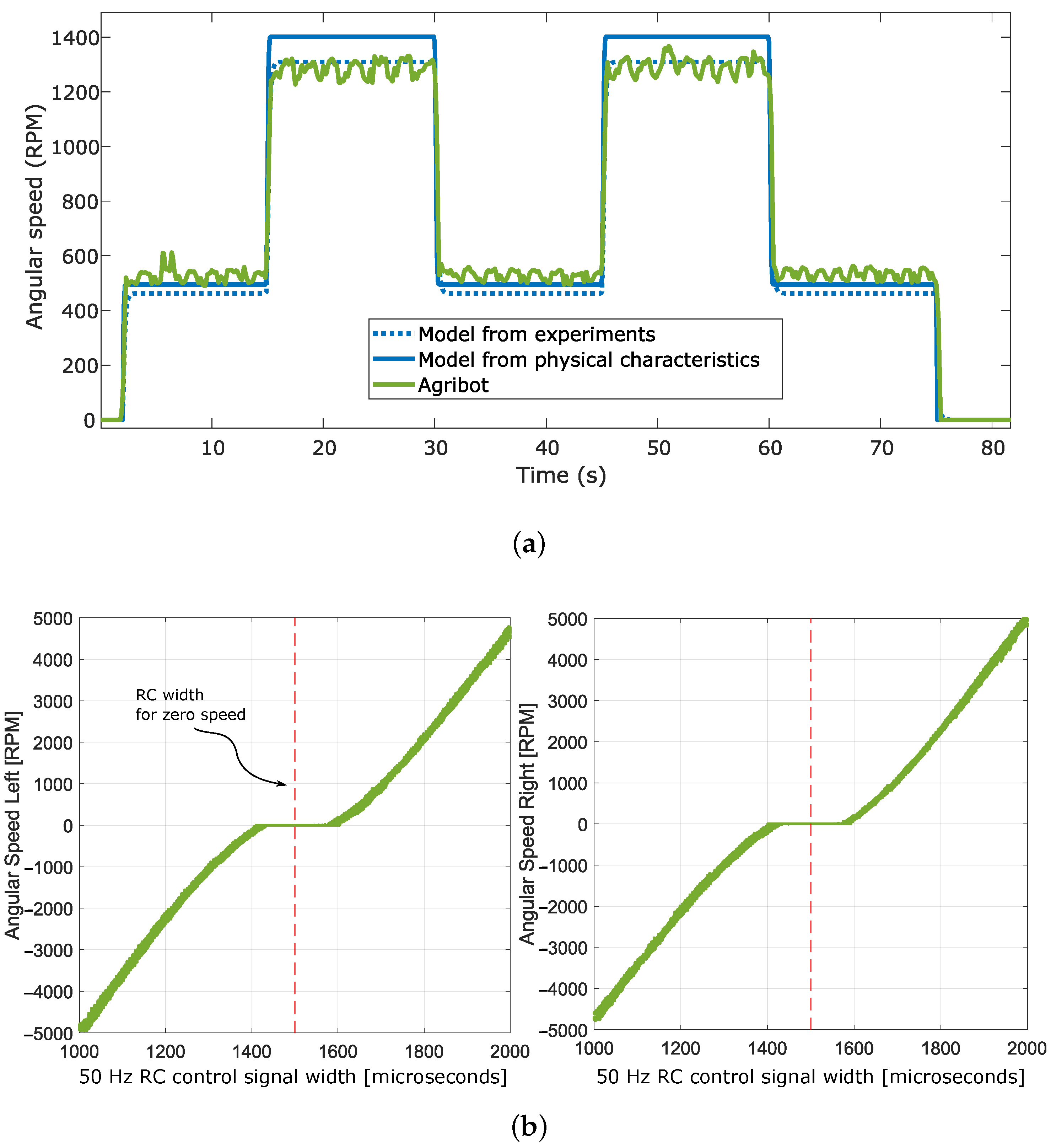
Notice that the static gain from the data sheet (Ampflow dc motors) is rad/s/V. The time constant and transport delay must be obtained from measurements because they depend on the utilization conditions of the system. Figure 5a shows a sample of model validation. In this test, repeated step changes in the control signal (voltage) were performed using the Agribot and then applied to the model tuned from measurements and computed from the data sheet using (15). The real system, composed of the drive, motor, and gearbox, also exhibits a non-negligible non-linearity consisting of a dead zone (dead-band), as presented in Figure 5b. This non-linearity imposes that the motor starts only when the controller’s control signal exceeds of its nominal value. Otherwise, it remains locked. We added the behaviour of the dead zone and the transport delay (35) to the model for emulation. It is common to intentionally implement this kind of dead zone directly in the drive to prevent the robot from moving when unnecessary and in case of wrong or biased zero calibration.

Figure 5.
Sample of open-loop test results and the motors’ model validation. (a) Simulation of angular speed versus measurements on the Agribot; (b) Angular speed of motors versus RC control signal width.
3.2. Implementation of Motors’ Speed Control
Considering the presence of non-negligible delays in the transfer function of the motors, we opted to use proportional and integral controllers (PI) for the speed control. The discrete version of each speed controller has been implemented using
with
and
where is the voltage to be applied to the motor, and are the instantaneous and integral speed errors, is the sampling period of the controller, and and are the controller parameters obtained using (16) and (17), (18) and (19), or (20) and (21). Two sets of parameters have been obtained, with the first set using the characteristics of the Qube servo 2 and the second using the characteristics of the motors of the Agribot, adding the transport delay observed in the real system. We employ the first-order approximation defined by (15) for the initial tuning of controllers.
3.3. Implementation of Path Tracking Strategy
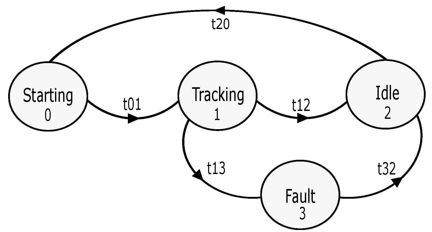
The path tracking strategy has been implemented based on the formulation presented in (27) and (33), and considering trajectories predefined using MATLAB and recorded in a CSV file as column vectors for . The file entry defining the path to be followed by the robot is read using an index k, controlled by a finite-state machine (FSM) with four states representing four working modes for the robot: 0: starting, 1: tracking, 2: idle, and 3: fault, as shown in Figure 6.

Figure 6.
Finite-state machine (FSM) to control the working modes of the Agribot.
In the starting mode, the reference, , is fixed to the first point of the planned trajectory, and the controllers of the angular speed of motors and the controller of linear velocity are enabled. The controller of yaw velocity is disabled to prevent an uncontrolled start. The FSM evolves to tracking mode when the robot starts moving (t01). In the tracking mode, the reference, , is updated using the sampling time of the controller, , by increasing the index, k, allowing the subsequent points of the trajectory to be read. The controllers of the angular speed of motors and the controllers of linear and yaw velocities are enabled. The FSM evolves from tracking to idle mode when the robot approaches the end position of the trajectory or when it covers a predefined distance (t12). The system remains ready to restart with the same or a new trajectory by moving to the starting mode (t20). If the position error or the angular or linear speed exceeds predefined maximum values, the FSM evolves from tracking to fault mode (t13). The system remains in fault mode until the robot operator provides an acknowledgement signal. Then, the FSM evolves to idle mode (t32). In idle mode, the reference, , is set to the robot’s actual position, all controllers are disabled, and the control output of the angular speed of motors is set to zero. The FSM enables the implementation of multiple sequences of movement and stationary work that could be particularly useful when the robot must accomplish tasks including periods of operations at specific locations, e.g., taking samples, measuring some parameters of soil, or performing a local intervention on crops.
4. Experimental Results
We present in this section the results of the angular speed control, the path tracking in HIL real-time emulation, and the experimental test using the Agribot.
4.1. Real-Time Emulation and Experiments of Angular Speed Control
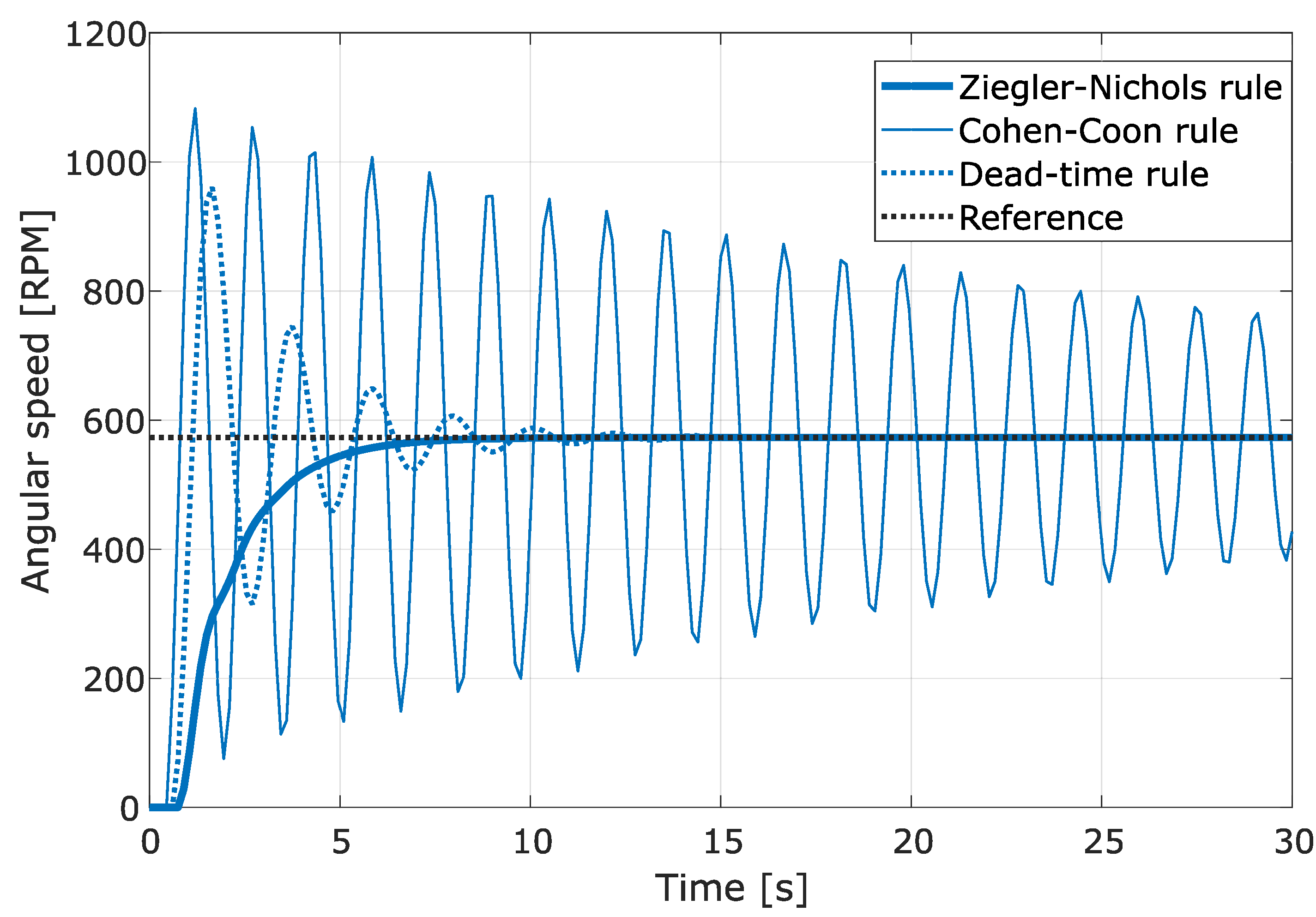
We employed the same formulation used in the previous section for tuning speed controllers using the parameters of the robot as defined in Table 1, and the first-order transfer function approximation with transport delay (35) obtained for the Agribot and the emulation using the Qube servo 2. We evaluated the response by using the three tuning methods mentioned in the previous section, as shown in Figure 7, and for this specific case, the Ziegler–Nichols and the dead-time rules allow acceptable step responses with similar settling times to be obtained, the first with over-damped and the second with under-damped behaviours. From the results obtained, the Cohen–Coon rule gives a controller tuning with a higher proportional gain that results in a response with significant overshoot and slow damping. It is therefore worth highlighting that implementing a controller with high proportional gain could be problematic when the sample time is long, as in the case under study.

Figure 7.
Comparison of angular speed control using different tuning methods (Ts = 150 ms).
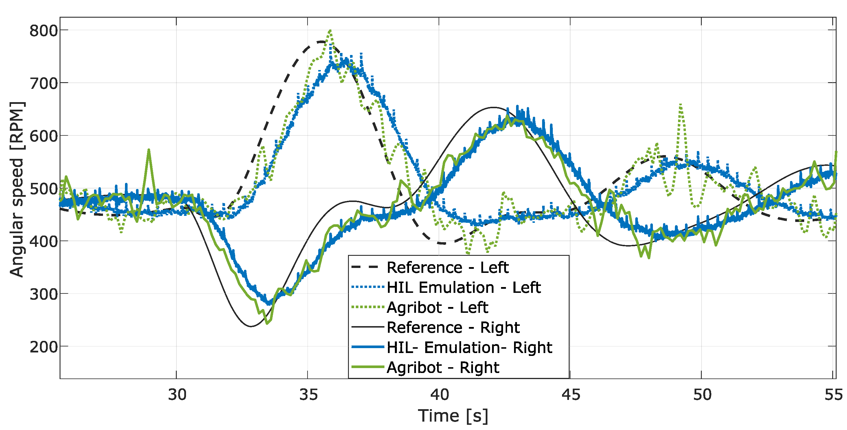
The results for the control of the two motors of the robot by imposing different speed profiles are presented in Figure 8.

Figure 8.
Comparison of angular speed control results by emulation and by experiments with the Agribot using Ziegler–Nichols tuning of PI controllers.
These results were obtained by fine-tuning from Ziegler–Nichols rule initial tuning, which allowed us to obtain a faster response. It can be observed that the results obtained by emulation fit with those of experiments using the Agribot platform. In these tests, the sample period of the speed controller was set to = 150 ms, and the controller was tuned using the Ziegler–Nichols rule. We employed the Ziegler–Nichols rule in the next tests; however, the dead-time rule could be a good choice for speed control in systems with significant delays as was the case with the robot under study.
4.2. Real-Time Emulation of Path Tracking
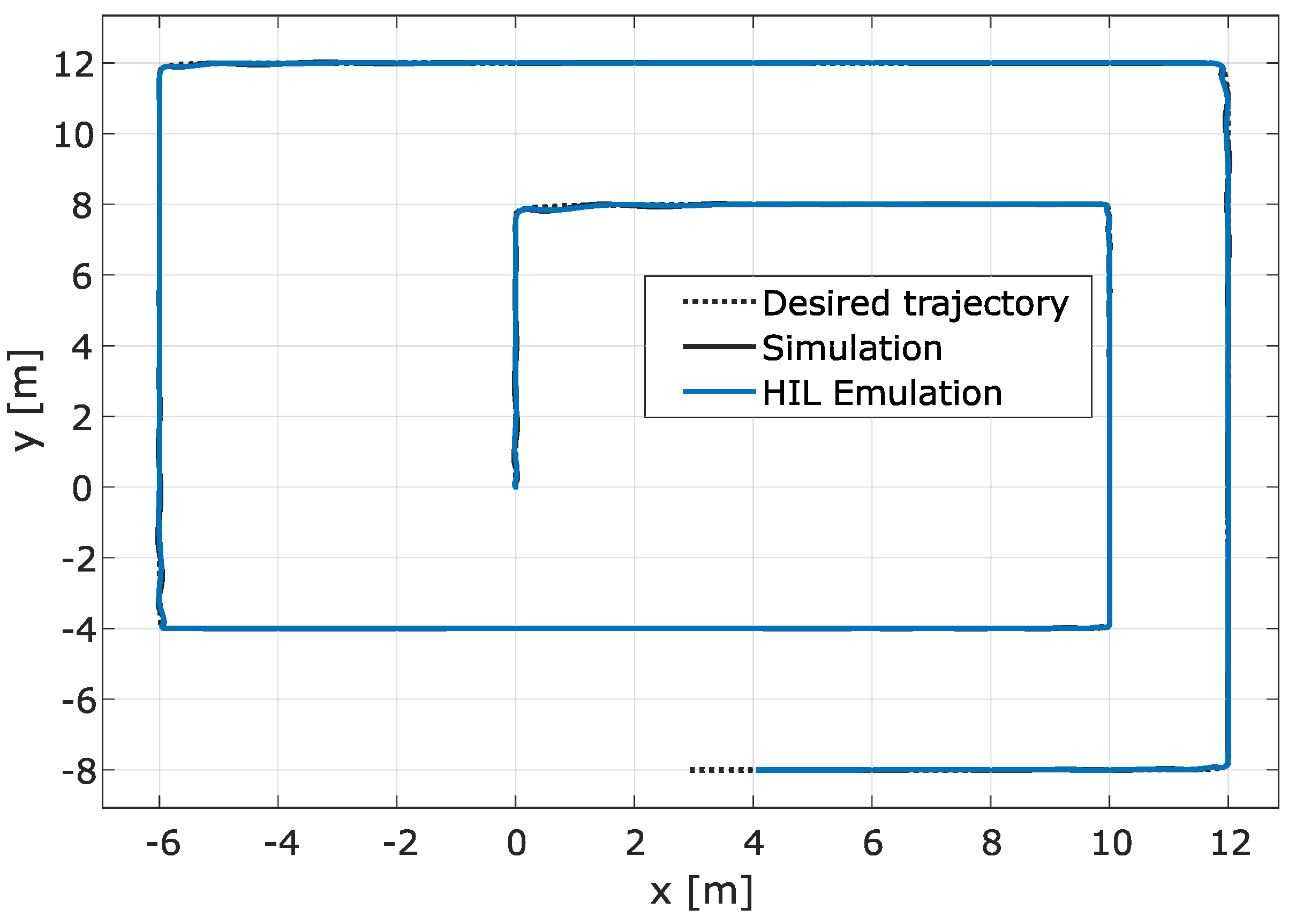
To validate the model and the path tracking strategy before testing it on the robot, we implemented and evaluated different trajectories, including saw-tooth, spiral, rectangular, circular, and eight-shaped paths.
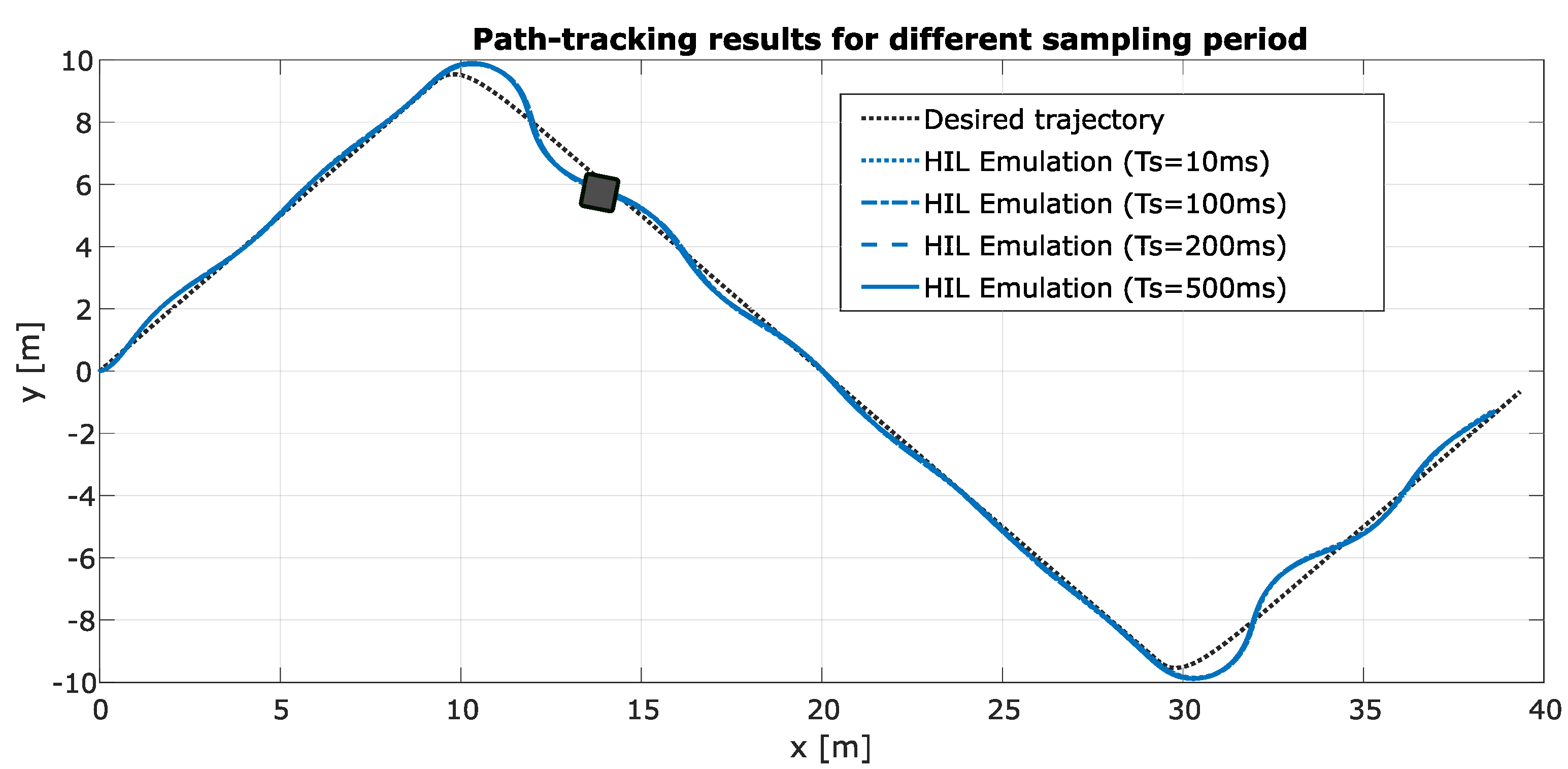
Figure 9 presents the saw-tooth path tracking results in emulation using different sampling periods (). These results confirm that the system keeps an acceptable dynamic behaviour even when using a high sampling period, i.e., ms. It can be observed that the robot deviates from the reference at the corners of the trajectory, but it is reoriented to follow the desired path. We employed in these tests the formulation from (22) and (24), with the following parameters: , , and . These parameters were tuned from those proposed in [37].

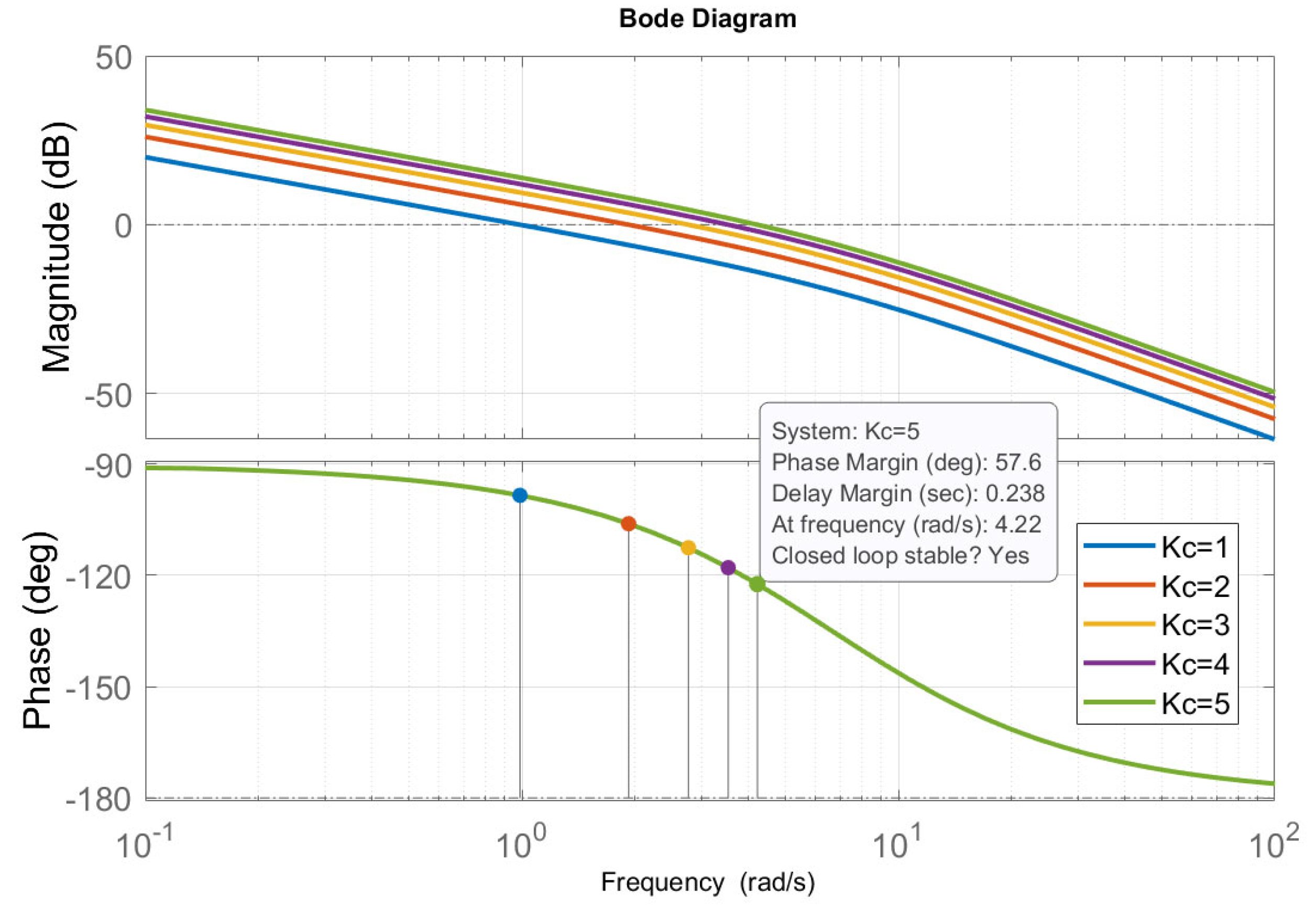
As a second test, we implemented a trajectory in the form of a spiral that imposes heading angles in all quadrants. This test ed us to verify the correct operation of the path tracking strategy as described in the previous section, using the formulation from (27) and (33). The controller gains were set to and . This tuning for angle control allows tolerating delays of s higher, enough compared to the transport lag of the system ( s). As illustrated in Figure 10, the system remains stable even for .

Figure 10.
Bode plot for different tuning of angle control gain .
However, the delay margin is reduced too close to the transport lag of the system ( ms, ms). In this case, the controller causes the robot to move forward as expected but zigzag around the trajectory. This also produces higher control effort, i.e., abrupt changes in control signals (speed references and voltages). The results of spiral trajectory tracking using the formulation from (27) and (33) for orientation and linear velocity control are presented in Figure 11. These results confirm the proper trajectory tracking in simulation and HIL real-time emulation.

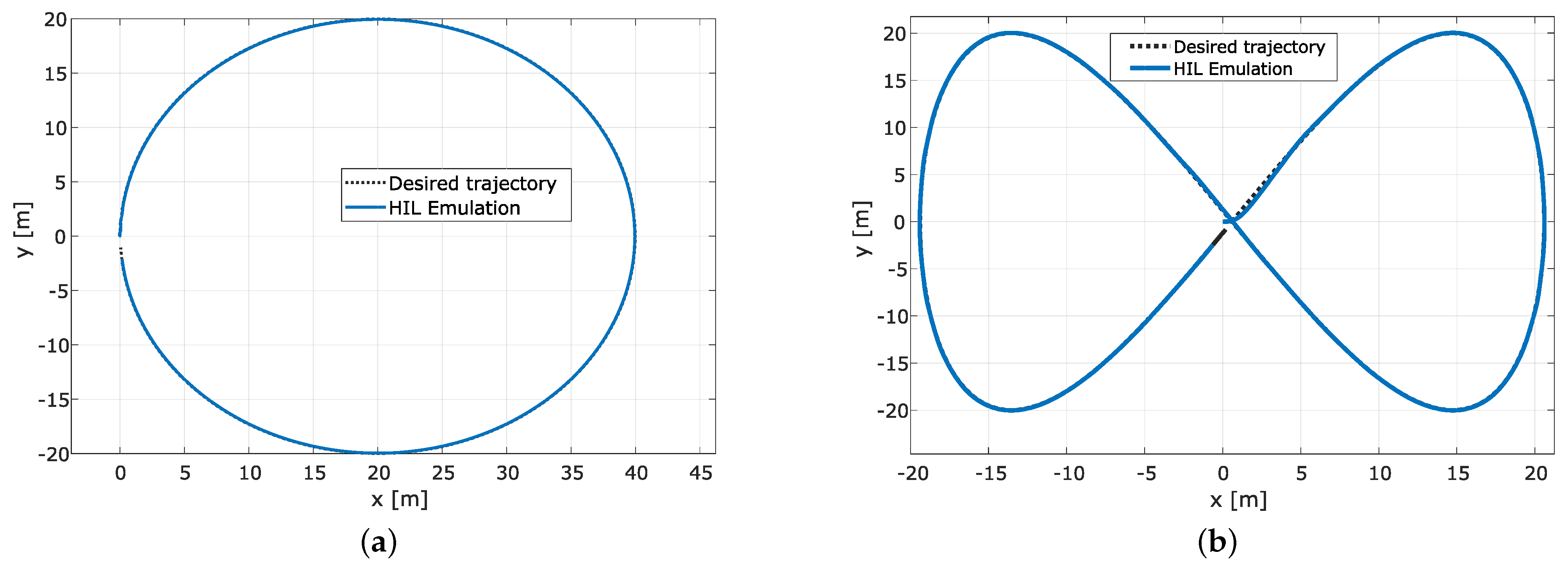
We implemented and tested circular and eight-shaped (Lissajous) paths as examples of closed trajectories commonly employed to validate the performance of path tracking strategies. The eight-shaped Lissajous path was implemented as and , where is the amplitude of displacement in x and y, and the velocity in rad/s. Figure 12a presents path tracking results for a circular shape and Figure 12b for an eight-shaped trajectory (with m), confirming the robot’s correct and almost perfect behaviour.

We can observe a transient deviation of 5 cm and a steady-state error of cm. These errors are negligible compared to the robot’s size with an axle track () of cm. It is worth highlighting that in emulation, we neglect the effects of the robot’s dynamics and external parameters and perturbations, e.g., changes in friction coefficient and slope and imperfections of ground. These assumptions allow, in emulation, significant performances that can not be obtained using the real setup.
4.3. Experiments of Path Tracking with the Agribot
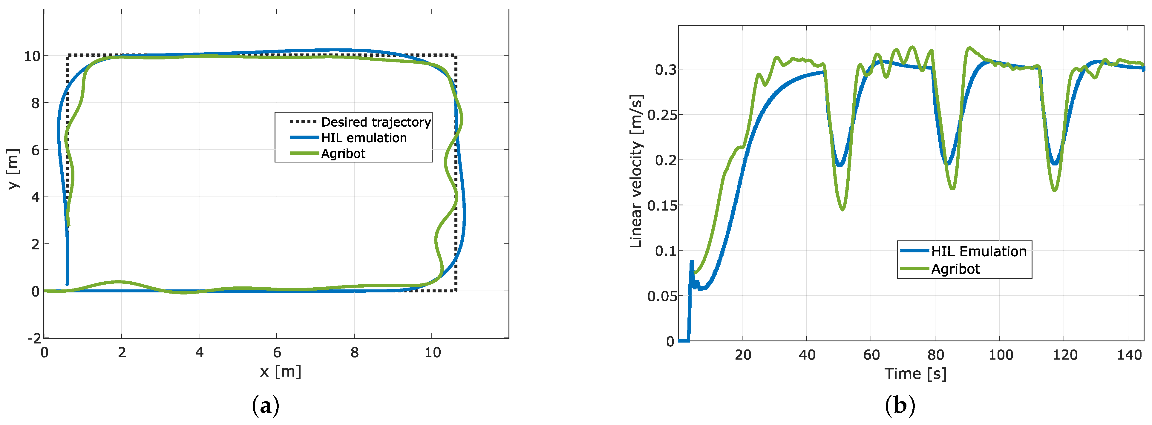
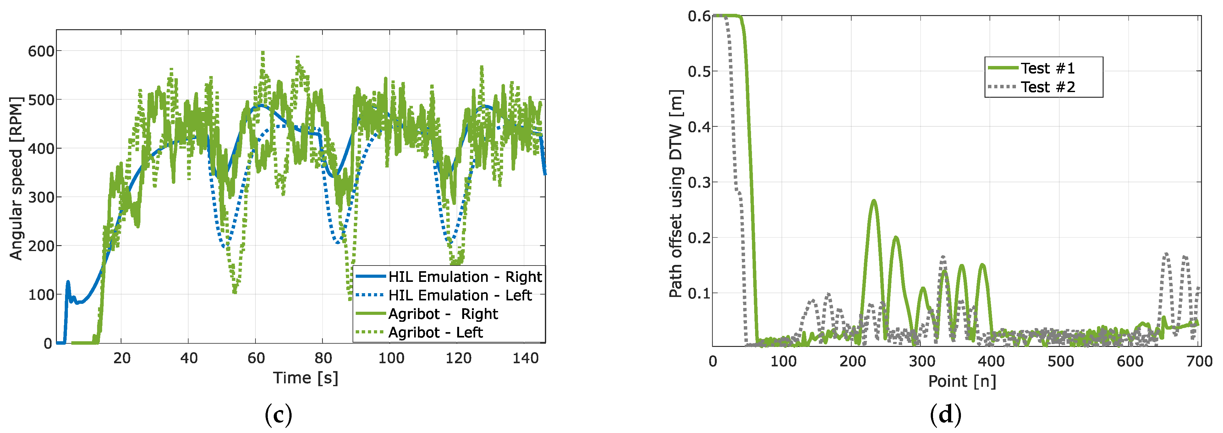
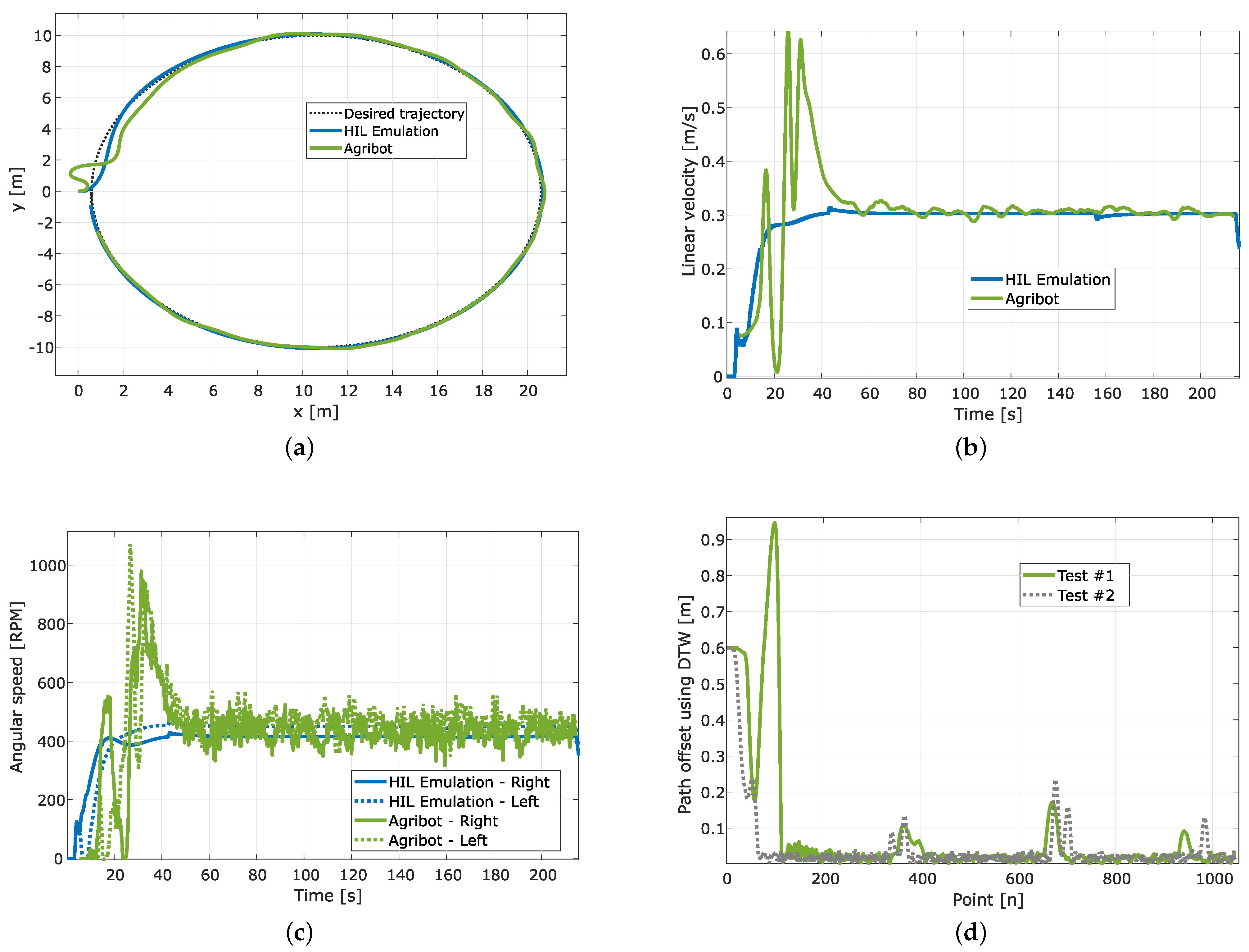
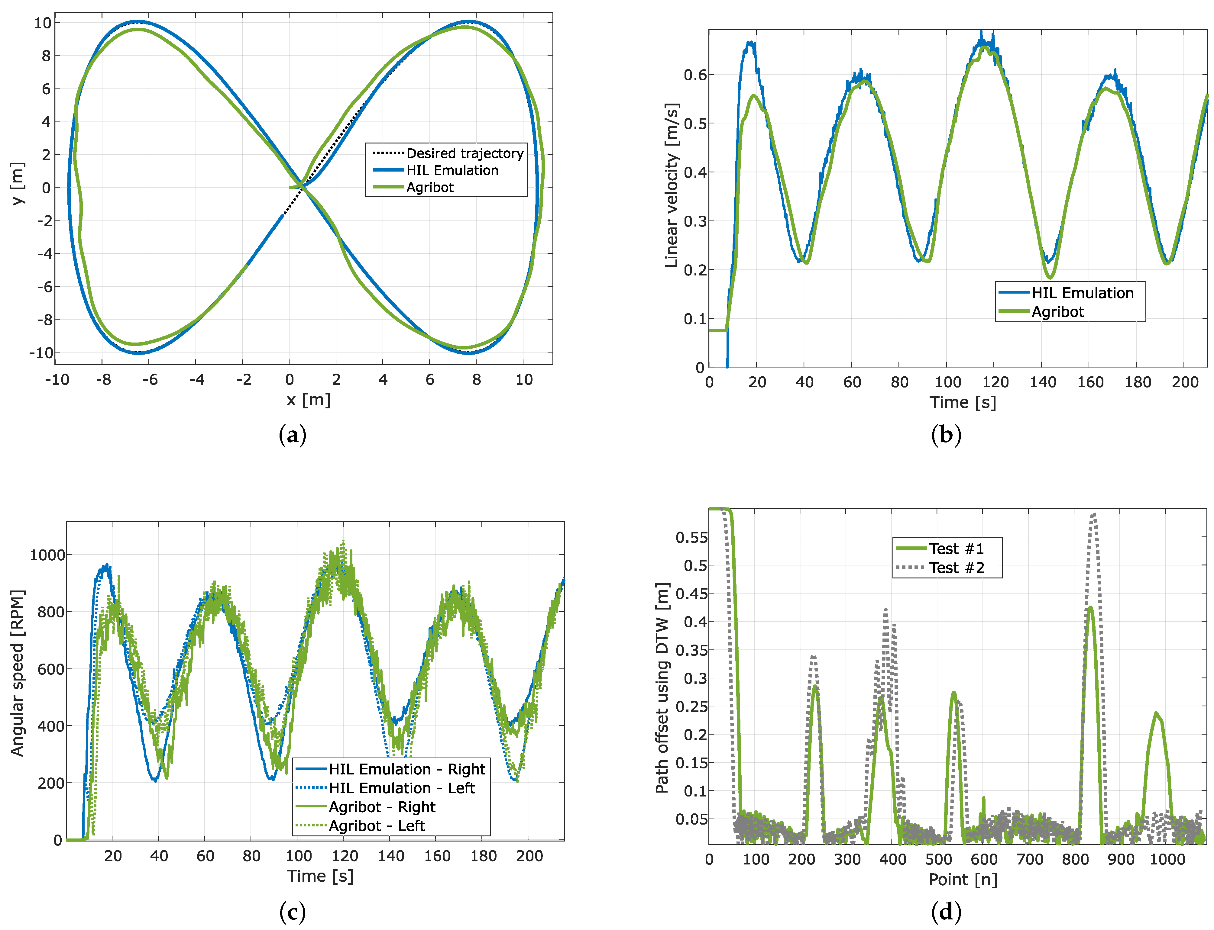
After evaluating the correct behaviour of the implemented strategy in simulation and HIL real-time emulation, we performed several tests using the Agribot platform in outdoor operation at the University of Quebec at Trois-Rivieres campus. We present, in Figure 13, Figure 14 and Figure 15, three samples of experimental results compared to the HIL emulation results.
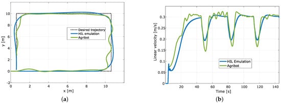

Figure 13.
Experimental results for rectangular trajectory. (a) Path tracking; (b) Linear velocity of the Agribot; (c) Angular speed of the motors; (d) Path offset computed using dynamic time warping.

Figure 14.
Experimental results for circular trajectory. (a) Path tracking; (b) Linear velocity of the Agribot; (c) Angular speed of the motors; (d) Path offset computed using dynamic time warping.

Figure 15.
Experimental results for eight-shaped trajectory. (a) Path tracking; (b) Linear velocity of the Agribot; (c) Angular speed of the motors; (d) Path offset computed using dynamic time warping.
The first example corresponds to a rectangular trajectory, the second to a circular trajectory, and the third to an eight-shaped trajectory. For the three cases, the sample time was set to ms, and the trajectories were generated to obtain, in steady state, a mean linear velocity of m/s. The plots for each test show the robot’s position () and desired path (, ), the robot’s linear velocity (v), the motors’ angular speed ( and ), and the path tracking error presented as a path offset. As observed in the plots of Figure 13a, Figure 14a and Figure 15a, the pathtracking is performed well in the three cases, and the robot can follow the planned trajectory. It is evident, from these results, that the path tracking error is more significant in the rectangular path because of the right angle changes the robot must accomplish. This is also reflected in the linear velocity (Figure 13b), which is reduced while the robot turns. In contrast, for the circular path (Figure 14b), once the robot reaches the correct alignment, it keeps an almost constant linear velocity close to the expected m/s. Furthermore, for the eight-shaped path (Figure 15a), the linear velocity reflected the correct behaviour of the robot, as is presented in Figure 15b. Following the same consideration, as illustrated in Figure 13c, Figure 14c and Figure 15c, the changes in the angular speed of motors are more significant for the rectangular trajectory. It is worth highlighting that, for the circular path, important changes in the angular speed appear while the robot is in the starting phase, but in the tracking phase, the motor speeds present small changes.
5. Discussion
This work allowed us to verify the advantage of using real-time hardware-in-the-loop emulation of agricultural robots for the preliminary evaluation of path tracking strategies using only the information of the angular speed of motors and yaw angular velocity of the robot. The experiments with an Agribot platform confirmed the results obtained by real-time HIL emulation with high similarity. Thus, using the HIL emulation to prepare and test control strategy variants and tuning before the evaluation using real hardware is not only possible but trustworthy. However, we must mention that it is almost impossible to reproduce in emulation external conditions that can affect the robot’s behaviour in a real environment. The proposed and implemented path tracking strategy works well for different types of trajectories, e.g., circular, eight-shaped, rectangular, spiral, and saw-tooth. In fact, in experimental tests for outdoor operation, the steady-state error of tracking is limited to values lower than the axle track of the robot (). To confirm this, we computed the path offset corresponding to the distance between desired path and the one followed by the robot using dynamic time warping (DTW) [40,41]. We plotted the results in Figure 13d, Figure 14d and Figure 15d. We include in this analysis a second tuning (Test #2 in each figure) for the angular speed controllers by increasing the integral constant () and by reducing the proportional gain (). The results suggest that improving the inner loop of angular speed control by fine-tuning accelerates the response and reduces the mean path tracking error. However, it produces more effort control.
The performance of the path tracking was compared to recent research works that considered similar applications and provided experimental result data. We must admit that the comparison is not easy to make because the characteristics of the vehicles and the type of tests are different from one publication to another. We have normalized the tracking error (path offset) with respect to the vehicle’s width (axle track) to facilitate the comparison and presented it as a relative path offset (39).
We compared the results of this work with those obtained by using an adaptive dynamic controller with parameters updating [22], an active disturbance rejection controller with observer based on an extended Kalman filter [23], a Takagi–Sugeno–Kang (TSK) type-2 fuzzy neural network (T2FNN) with sliding mode control (SMC) [24], a robust adaptive fuzzy variable structure [25], and a fuzzy dynamic sliding mode controller [26]. The results of this comparison are summarized in Table 2. We can corroborate that the proposed path tracking strategy performs similarly or better than more sophisticated methods reported in the literature. It is worth highlighting that some works used small robots and tested the strategies in indoor conditions that favour path tracking [22,25,26].

Table 2.
Comparison of relative path offset using different path tracking strategies.
6. Conclusions
This paper proposed a methodology for real-time HIL emulation of path tracking in agricultural robots (Agribot). The proposed emulation employs MATLAB/Simulink for the implementation of the kinematic models, angular speed controllers, and path tracking strategy, as well as the Qube servo 2, from Quanser, for the emulation of the traction system of the robot. This study provides details for implementing a path tracking strategy using only three pieces of information: the angular speeds of wheels from encoders, and the yaw angular velocity of the robot, from an inertial measurement unit (IMU). It also brings the analysis of controller tuning in the case of low-latency control applied to traction systems with non-linearities and non-negligible transport delays. Experiments using an Agribot platform operated outdoors confirmed the simulation and real-time HIL emulation results.
Based on the emulation and experimental results and the comparative analysis presented in the previous section, it is possible to confirm, on the one hand, that the proposed HIL emulation can be used for the preliminary evaluation of path tracking strategies in Agribots. On the other hand, it can also be confirmed that the proposed low-complexity kinematic-based strategy using low-cost hardware allows us to obtain comparable or better results than those obtained with more sophisticated control strategies.
Current research includes the analysis of the impact of environmental changes and perturbations on path tracking, their automated detection and mitigation by low-complexity control strategies. These works focus on improving the precision of path tracking in semi-autonomous agricultural robots while keeping low-cost implementation and adapting online models and controllers’ tuning. We consider in the next steps the implementation of controllers using software/hardware co-design to reduce latency issues associated with pure software solutions.
Author Contributions
Conceptualization, I.J.M., D.O., D.C.-A. and A.C.; methodology, I.J.M., D.O., D.C.-A. and A.C.; software, I.J.M. and D.O.; validation, I.J.M. and D.O.; formal analysis, I.J.M., D.O. and A.C.; investigation, I.J.M., D.O., D.C.-A. and A.C.; resources, A.C.; data curation, I.J.M., D.O. and A.C.; writing—original draft preparation, I.J.M., D.O., D.C.-A. and A.C.; writing—review and editing, I.J.M., D.O., D.C.-A. and A.C.; visualization, I.J.M., D.O. and A.C.; supervision, A.C.; project administration, A.C.; funding acquisition, A.C. All authors have read and agreed to the published version of the manuscript.
Funding
This research received no external funding.
Data Availability Statement
Data available on request.
Acknowledgments
The authors would like to thank the “Ministère des Relations internationales et de la Francophonie—MRIF—du Québec”, MITACS, EduCanada, and the Natural Sciences and Engineering Research Council of Canada—NSERC for the financial support.
Conflicts of Interest
The authors declare no conflict of interest.
References
- United Nations Department of Economic and Social Affairs. The Sustainable Development Goals Report 2022; United Nations: New York, NY, USA, 2022. [Google Scholar]
- Ghobadpour, A.; Monsalve, G.; Cardenas, A.; Mousazadeh, H. Off-Road Electric Vehicles and Autonomous Robots in Agricultural Sector: Trends, Challenges, and Opportunities. Vehicles 2022, 4, 843–864. [Google Scholar] [CrossRef]
- Skrucany, T.; Harantova, V.; Kendra, M.; Barta, D. Reducing Energy Consumption by Passenger Car with Using of Non-Electrical Hybrid Drive Technology. Adv. Sci. Technol. Res. J. 2017, 11, 166–172. [Google Scholar] [CrossRef]
- Alegre, Y.C.; Podewils, T.A.; Peñaloza, E.A.G.; de Lima, S.; Leston, L.A. Characterization of Physical Parameters of an Agricultural Electric Vehicle based on the Dynamic Analysis in a Simulated Environment. In Proceedings of the 2021 IEEE 15th International Conference on Semantic Computing (ICSC), Laguna Hills, CA, USA, 27–29 January 2021; pp. 380–385. [Google Scholar] [CrossRef]
- Caban, J.; Vrabel, J.; Sarkan, B.; Zarajczyk, J.; Marczuk, A. Analysis of the market of electric tractors in agricultural production. MATEC Web Conf. 2018, 244, 03005. [Google Scholar] [CrossRef]
- Kang, C.M.; Lee, S.H.; Chung, C.C. Multirate Lane-Keeping System with Kinematic Vehicle Model. IEEE Trans. Veh. Technol. 2018, 67, 9211–9222. [Google Scholar] [CrossRef]
- Klepikov, V.; Semikov, O. Modeling The Dynamic Processes of The Electric Drive of Electric Vehicle While Wheels are Slipping. In Proceedings of the 2020 IEEE Problems of Automated Electrodrive, Theory and Practice (PAEP), Kremenchuk, Ukraine, 21–25 September 2020; pp. 1–6. [Google Scholar] [CrossRef]
- Filipescu, A.; Minzu, V.; Dumitrascu, B.; Filipescu, A.; Minca, E. Trajectory-tracking and discrete-time sliding-mode control of wheeled mobile robots. In Proceedings of the 2011 IEEE International Conference on Information and Automation, Shenzhen, China, 6–8 June 2011; pp. 27–32. [Google Scholar] [CrossRef]
- Wang, X.; Sun, W. Trajectory Tracking of Autonomous Vehicle: A Differential Flatness Approach with Disturbance-Observer-Based Control. IEEE Trans. Intell. Veh. 2023, 8, 1368–1379. [Google Scholar] [CrossRef]
- Caban, J.; Nieoczym, A.; Dudziak, A.; Krajka, T.; Stopková, M. The Planning Process of Transport Tasks for Autonomous Vans—Case Study. Appl. Sci. 2022, 12, 2993. [Google Scholar] [CrossRef]
- Misztal, W. The Impact of Perturbation Mechanisms on the Operation of the Swap Heuristic. Arch. Automot. Eng. Arch. Motoryz. 2019, 86, 27–39. [Google Scholar] [CrossRef]
- Wu, H.M.; Zaman, M.Q. LiDAR Based Trajectory-Tracking of an Autonomous Differential Drive Mobile Robot Using Fuzzy Sliding Mode Controller. IEEE Access 2022, 10, 33713–33722. [Google Scholar] [CrossRef]
- Huang, J.; Junginger, S.; Liu, H.; Thurow, K. Indoor Positioning Systems of Mobile Robots: A Review. Robotics 2023, 12, 47. [Google Scholar] [CrossRef]
- Yi, J.; Wang, H.; Zhang, J.; Song, D.; Jayasuriya, S.; Liu, J. Kinematic Modeling and Analysis of Skid-Steered Mobile Robots with Applications to Low-Cost Inertial-Measurement-Unit-Based Motion Estimation. IEEE Trans. Robot. 2009, 25, 1087–1097. [Google Scholar] [CrossRef]
- Ge, Z.; Man, Z.; Wang, Z.; Bai, X.; Wang, X.; Xiong, F.; Li, D. Robust adaptive sliding mode control for path tracking of unmanned agricultural vehicles. Comput. Electr. Eng. 2023, 108, 108693. [Google Scholar] [CrossRef]
- Liu, Q.; Cong, Q. Kinematic and dynamic control model of wheeled mobile robot under internet of things and neural network. J. Supercomput. 2022, 78, 8678–8707. [Google Scholar] [CrossRef] [PubMed]
- Chen, R.; Yang, C.; Ma, Y.; Wang, W.; Wang, M.; Du, X. Online learning predictive power coordinated control strategy for off-road hybrid electric vehicles considering the dynamic response of engine generator set. Appl. Energy 2022, 323, 119592. [Google Scholar] [CrossRef]
- Ghobadpour, A.; Cardenas, A.; Monsalve, G.; Mousazadeh, H. Optimal Design of Energy Sources for a Photovoltaic/Fuel Cell Extended-Range Agricultural Mobile Robot. Robotics 2023, 12, 13. [Google Scholar] [CrossRef]
- Małek, A.; Caban, J.; Dudziak, A.; Marciniak, A.; Ignaciuk, P. A Method of Assessing the Selection of Carport Power for an Electric Vehicle Using the Metalog Probability Distribution Family. Energies 2023, 16, 5077. [Google Scholar] [CrossRef]
- Yan, C.; Shao, K.; Wang, X.; Zheng, J.; Liang, B. Reference Governor-Based Control for Active Rollover Avoidance of Mobile Robots. In Proceedings of the 2021 IEEE International Conference on Systems, Man, and Cybernetics (SMC), Melbourne, Australia, 17–20 October 2021; pp. 429–435. [Google Scholar] [CrossRef]
- Taghia, J.; Stanley Lam, X.W.; Katupitiya, J. A sliding mode controller with a nonlinear disturbance observer for a farm vehicle operating in the presence of wheel slip. Auton. Robot. 2017, 41, 71–88. [Google Scholar] [CrossRef]
- Martins, F.N.; Celeste, W.C.; Carelli, R.; Sarcinelli-Filho, M.; Bastos-Filho, T.F. An adaptive dynamic controller for autonomous mobile robot trajectory tracking. Control Eng. Pract. 2008, 16, 1354–1363. [Google Scholar] [CrossRef]
- Sebastian, B.; Ben-Tzvi, P. Active Disturbance Rejection Control for Handling Slip in Tracked Vehicle Locomotion. J. Mech. Robot. 2019, 11, 021003. [Google Scholar] [CrossRef]
- Kayacan, E.; Kayacan, E.; Ramon, H.; Kaynak, O.; Saeys, W. Towards Agrobots: Trajectory Control of an Autonomous Tractor Using Type-2 Fuzzy Logic Controllers. IEEE/ASME Trans. Mechatron. 2015, 20, 287–298. [Google Scholar] [CrossRef]
- Begnini, M.; Bertol, D.W.; Martins, N.A. A robust adaptive fuzzy variable structure tracking control for the wheeled mobile robot: Simulation and experimental results. Control Eng. Pract. 2017, 64, 27–43. [Google Scholar] [CrossRef]
- Hwang, C.L.; Yang, C.C.; Hung, J.Y. Path Tracking of an Autonomous Ground Vehicle with Different Payloads by Hierarchical Improved Fuzzy Dynamic Sliding-Mode Control. IEEE Trans. Fuzzy Syst. 2018, 26, 899–914. [Google Scholar] [CrossRef]
- Campion, G.; Bastin, G.; Dandrea-Novel, B. Structural properties and classification of kinematic and dynamic models of wheeled mobile robots. IEEE Trans. Robot. Autom. 1996, 12, 47–62. [Google Scholar] [CrossRef]
- Siegwart, R.; Nourbakhsh, I.; Scaramuzza, D. Introduction to Autonomous Mobile Robots, 2nd ed.; Intelligent Robotics and Autonomous Agents Series; MIT Press: Cambridge, MA, USA, 2011. [Google Scholar]
- Stefek, A.; Pham, T.V.; Krivanek, V.; Pham, K.L. Energy Comparison of Controllers Used for a Differential Drive Wheeled Mobile Robot. IEEE Access 2020, 8, 170915–170927. [Google Scholar] [CrossRef]
- Kumar, P.; Bensekrane, I.; Merzouki, R. Power Consumption Modeling of Wheeled Mobile Robots with Multiple Driving Modes. IEEE Trans. Ind. Electron. 2023, 70, 10282–10291. [Google Scholar] [CrossRef]
- Monsalve, G.; Cardenas, A.; Acevedo-Bueno, D.; Martinez, W. Assessing the Limits of Equivalent Circuit Models and Kalman Filters for Estimating the State of Charge: Case of Agricultural Robots. Energies 2023, 16, 3133. [Google Scholar] [CrossRef]
- Vantsevich, V.V.; Gorsich, D.J.; Paldan, J.R.; Ghasemi, M.; Moradi, L.; Letherwood, M. Terrain mobility performance optimization: Fundamentals for autonomous vehicle applications Part II. Computational simulation, implementation for mobility design, and validation. J. Terramech. 2022, 104, 59–85. [Google Scholar] [CrossRef]
- Aoki, N.; Ishigami, G. Hardware-in-the-loop Simulation for Real-time Autonomous Tracking and Landing of an Unmanned Aerial Vehicle. In Proceedings of the 2023 IEEE/SICE International Symposium on System Integration (SII), Atlanta, GA, USA, 17–20 January 2023; pp. 1–6. [Google Scholar] [CrossRef]
- Stączek, P.; Pizoń, J.; Danilczuk, W.; Gola, A. A Digital Twin Approach for the Improvement of an Autonomous Mobile Robots (AMR’s) Operating Environment—A Case Study. Sensors 2021, 21, 7830. [Google Scholar] [CrossRef] [PubMed]
- Ziegler, J.G.; Nichols, N.B. Optimum Settings for Automatic Controllers. J. Fluids Eng. 1942, 64, 759–765. [Google Scholar] [CrossRef]
- Cohen, G.H.; Coon, G.A. Theoretical Consideration of Retarded Control. Trans. Am. Soc. Mech. Eng. 2022, 75, 827–834. [Google Scholar] [CrossRef]
- Cornejo, J.; Magallanes, J.; Denegri, E.; Canahuire, R. Trajectory Tracking Control of a Differential Wheeled Mobile Robot: A Polar Coordinates Control and LQR Comparison. In Proceedings of the 2018 IEEE XXV International Conference on Electronics, Electrical Engineering and Computing (INTERCON), Lima, Peru, 8–10 August 2018; pp. 1–4. [Google Scholar] [CrossRef]
- Panigrahi, P.K.; Bisoy, S.K. Localization strategies for autonomous mobile robots: A review. J. King Saud Univ. Comput. Inf. Sci. 2022, 34, 6019–6039. [Google Scholar] [CrossRef]
- Monsalve, G.; Belhadj Ltaief, N.; Amoriya, V.; Cardenas, A. Kinematic Navigation Control of Differential Drive Agricultural Robot. In Proceedings of the 2022 IEEE International Conference on Electrical Sciences and Technologies in Maghreb (CISTEM), Tunis, Tunisia, 26–28 October 2022; Volume 4, pp. 1–6. [Google Scholar] [CrossRef]
- Paliwal, K.; Agarwal, A.; Sinha, S. A modification over Sakoe and Chiba’s dynamic time warping algorithm for isolated word recognition. In Proceedings of the ICASSP ’82. IEEE International Conference on Acoustics, Speech, and Signal Processing, Paris, France, 3–5 May 1982; Volume 7, pp. 1259–1261. [Google Scholar] [CrossRef]
- Berndt, D.J.; Clifford, J. Using Dynamic Time Warping to Find Patterns in Time Series. In Proceedings of the 3rd International Conference on Knowledge Discovery and Data Mining, Seattle, WA, USA, 31 July 1994; AAAIWS’94. AAAI Press: Washington, DC, USA, 1994; pp. 359–370. [Google Scholar]
Disclaimer/Publisher’s Note: The statements, opinions and data contained in all publications are solely those of the individual author(s) and contributor(s) and not of MDPI and/or the editor(s). MDPI and/or the editor(s) disclaim responsibility for any injury to people or property resulting from any ideas, methods, instructions or products referred to in the content. |
© 2023 by the authors. Licensee MDPI, Basel, Switzerland. This article is an open access article distributed under the terms and conditions of the Creative Commons Attribution (CC BY) license (https://creativecommons.org/licenses/by/4.0/).

