Article

Research on Yaw Moment Control System for Race Cars Using Drive and Brake Torques

1
Course of Mechanical Engineering, Tokai University, Kitakaname 4-4-1, Hiratsuka 259-1292, Japan
2
Course of Science and Technology, Tokai University, Kitakaname 4-4-1, Hiratsuka 259-1292, Japan
3
Research Institute of Science and Technology, Tokai University, Kitakaname 4-4-1, Hiratsuka 259-1292, Japan
4
Department of Electronic Robot Engineering, Aichi University of Technology, 50-2 Manori, Nishihasama-cho, Gamagori 443-0047, Japan
5
Department of Mechanical Engineering, Hokkaido University of Science, 7-Jo 15-4-1 Maeda, Sapporo 006-8585, Japan
6
Department of Mechanical Engineering, Tokyo University of Technology, 1404-1 Katakuramachi, Hachioji 192-0982, Japan
7
Department of Electrical Engineering, Fukuoka Institute of Technology, 3-30-1 Wajiro-Higashi, Fukuoka 811-0295, Japan
8
Faculty of Mechanical and Automotive Engineering Technology, University Malaysia Pahang, Pekan 26600, Malaysia
9
Department of Mechanical Systems Engineering, Tokai University, Kitakaname 4-4-1, Hiratsuka 259-1292, Japan
*
Author to whom correspondence should be addressed.
Vehicles 2023, 5(2), 515-534; https://doi.org/10.3390/vehicles5020029
Submission received: 13 January 2023 / Revised: 18 April 2023 / Accepted: 24 April 2023 / Published: 30 April 2023
(This article belongs to the Topic Vehicle Dynamics and Control)

Abstract

:
The yaw acceleration required for circuit driving is determined by the time variation of the yaw rate due to two factors: corner radius and velocity at the center of gravity. Torque vectoring systems have the advantage where the yaw moment can be changed only by the longitudinal force without changing the lateral force of the tires, which greatly affects lateral acceleration. This is expected to improve the both the spinning performance and the orbital performance, which are usually in a trade-off relationship. In this study, we proposed a yaw moment control technology that actively utilized a power unit with a brake system, which was easy to implement in a system, and compared the performance of vehicles equipped with and without the proposed system using the Milliken Research Associates moment method for quasi-steady-state analysis. The performances of lateral acceleration and yaw moment were verified using the same method, and a variable corner radius simulation for circuit driving was used to compare time and performance. The results showed the effectiveness of the proposed system.

1. Introduction

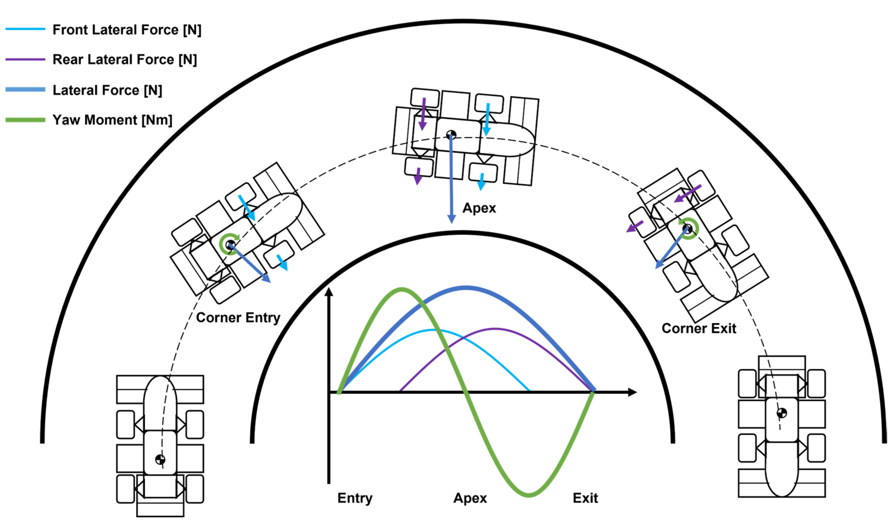
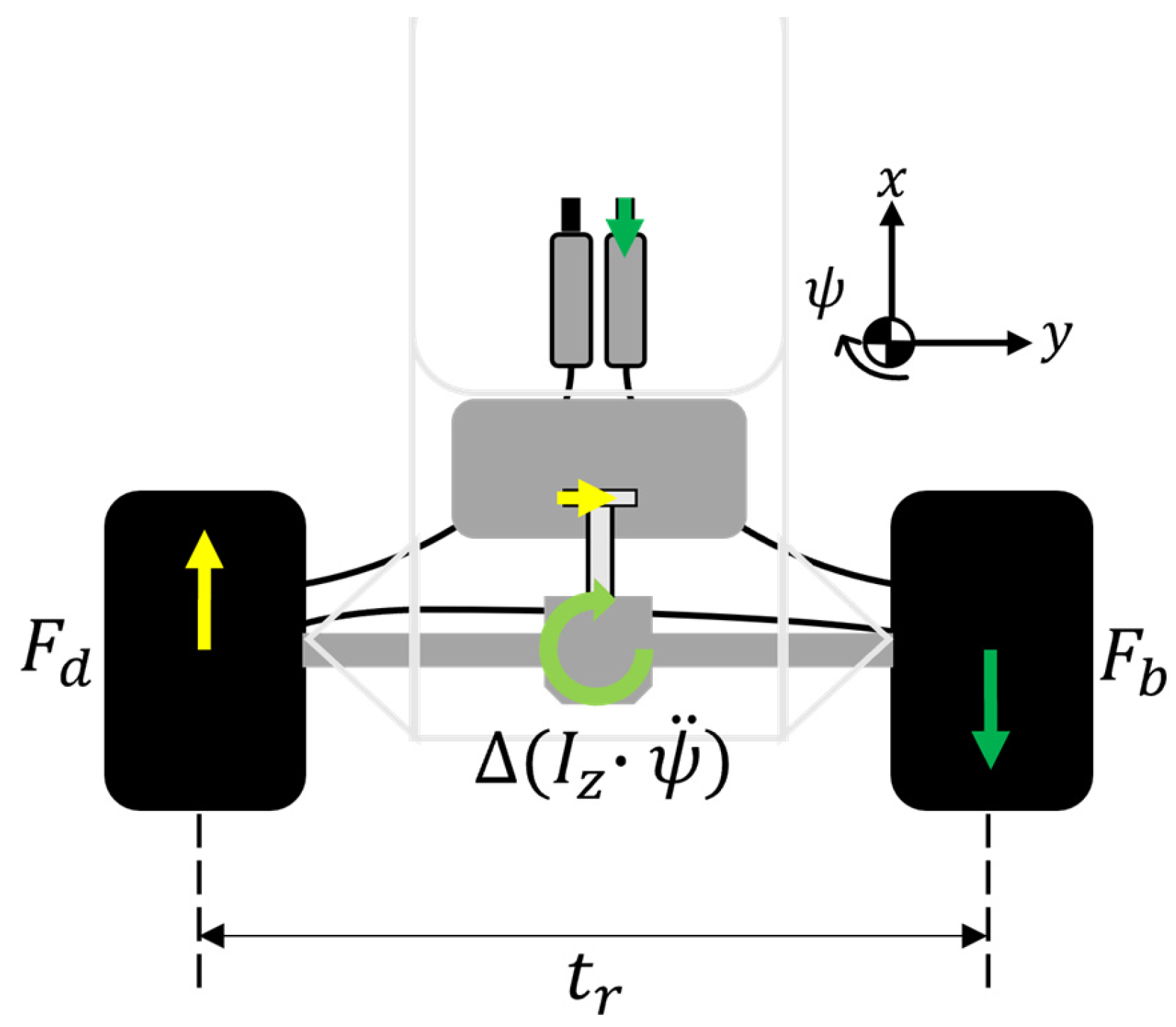
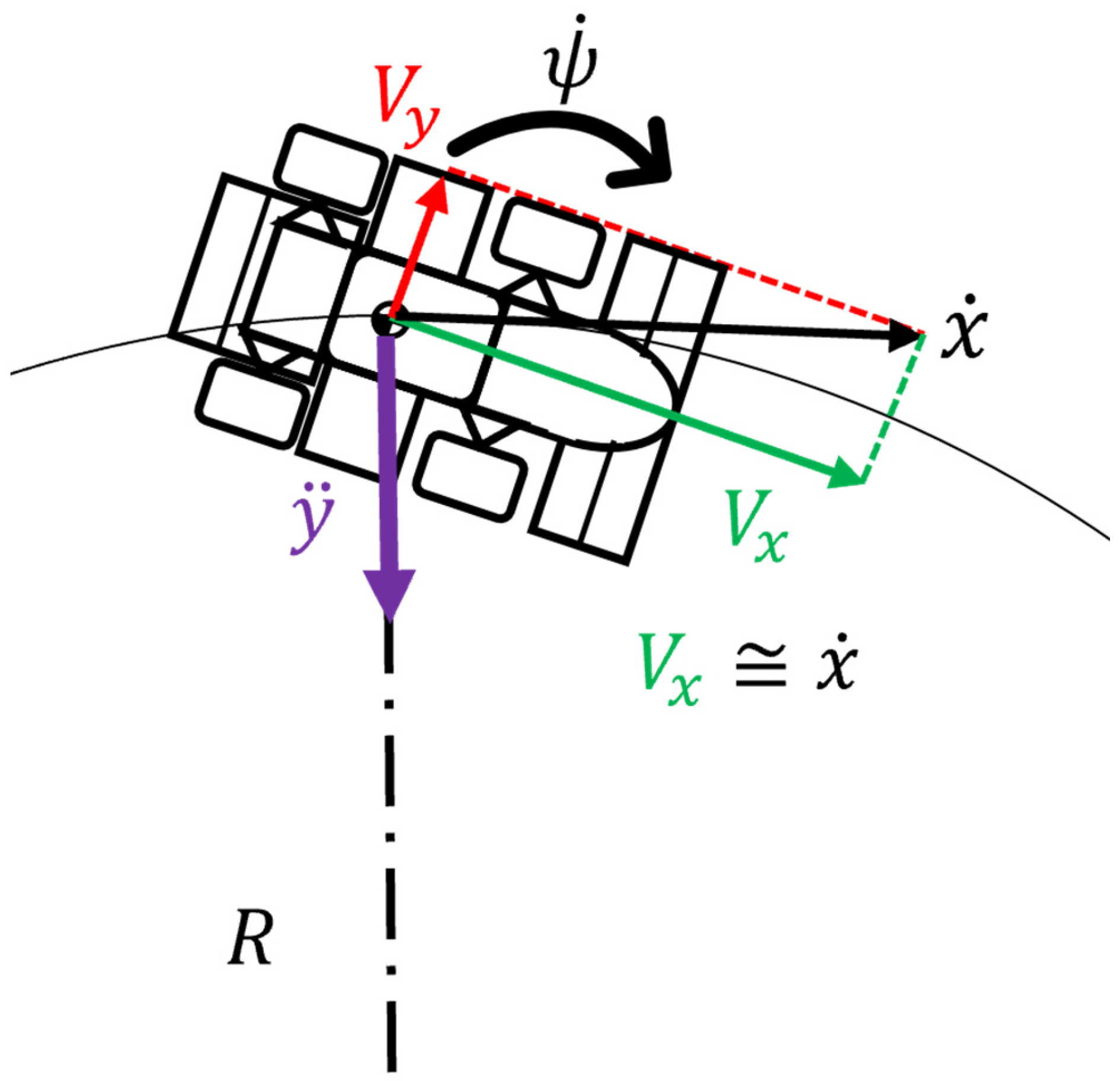
To improve the vehicle performance of race cars on circuits, we must consider not only the maximization of the friction ellipse, which is indicated by the longitudinal acceleration during braking/acceleration and the lateral acceleration during steady circle turns, but also the yaw rotational motion of the vehicle body itself. This is because in circuit driving with a series of various corner radii, the vehicle needs not only the orbital motion of the turning center, based on the lateral acceleration, owing to the generation of a cornering force balanced by centrifugal force, but also the spinning motion of the center of gravity position of the vehicle body to change its orientation in accordance with the track. For these spinning motions, yaw acceleration must be acquired, and a yaw moment must be generated in the vehicle. The yaw moment in a vehicle is mainly determined by three factors: longitudinal force, lateral force, and self-aligning torque of each of the four tires, as well as the position of the vehicle’s center of gravity, wheelbase, and front and rear track widths. In a conventional vehicle, the forces and moments generated by these four tires vary depending on the steering angle, throttle opening, brake pedal force, and vehicle characteristics in order to generate spinning and orbital rotation to make turns. However, there is a considerable trade-off between yaw acceleration for spinning motions and lateral acceleration for orbital motions. The required amount of yaw acceleration in circuit driving is determined by the time variation of the yaw velocity based on two factors: the corner radius and velocity at the center of gravity. Thus, when the lateral acceleration of the vehicle is increased for some reason, the turning speed of the vehicle is increased. The yaw rate, acceleration, and moment required, in this case, are higher. As shown in Figure 1, in a conventional vehicle, the source of the yaw moment is mostly the difference in the lateral force generation time between the front and rear, and the only way to offer the vehicle a high yaw moment is to reduce the lateral force of the rear tires. However, sacrificing the rear lateral force means that the overall cornering force and lateral acceleration of the vehicle are reduced. In circuits with a small corner radius, the superiority of yaw rotation motion performance is more pronounced, due to the greater yaw moment requirement.
In recent years, many control technologies have been researched and developed to improve these trade-offs. Previous studies can be broadly divided into two categories: lateral force control using tire slip angle and longitudinal force control using drive torque (torque vectoring). A typical example of the former is active rear-wheel steering. As the name suggests, this controls yaw moment by dynamically changing the rear tire slip angle, thereby changing the lateral force on the rear tires [1,2,3]. Since many vehicles have a longer wheelbase than track, it is expected that the yaw moment can be varied efficiently. However, the system’s characteristic of directly controlling the lateral force has a high impact on lateral acceleration, and if the yaw moment is to be used actively, as is the case for this purpose, the lateral force on the rear tires must be reduced, resulting in a significant reduction in the vehicle’s overall lateral acceleration. In the latter, torque vectoring control is actively studied in vehicles with four-wheel in-wheel motors in which all tires generate drive torque. In these systems, the yaw moment is directly controlled by controlling the motor torque of the four wheels, thereby varying the longitudinal forces [4,5,6,7,8]. Torque vectoring control has the advantage over active rear-wheel steering in that it does not significantly change the lateral forces on the tires, which have a large effect on lateral acceleration, and ideally, the yaw moment can be changed only by longitudinal forces. In aiming to actively use the yaw moment in this study, direct control of the driving force is considered more suitable than lateral force control using the slip angle, in terms of preventing a reduction in lateral acceleration.
In the field of front-wheel drive or rear-wheel drive vehicles, which are currently used in many racing categories, research is being conducted on torque vectoring control using active/semi-active differential mechanisms and on improving the driving force at corner exits [9,10]. This system can transmit torque to any wheel and generate yaw moment by controlling the locking torque and its direction using an actuator in a passive limited-slip differential mechanism, combined with an existing multi-disc clutch. The problem with these systems is the complexity of the mechanism, and there are few examples of their use in competition or commercial vehicles, due to the cost and weight. Due to these problems, there is a need for systems that can implement yaw moment control relatively easily, and research has been conducted on systems that generate yaw moment by applying brake torque to either wheel [11]. These systems have the advantage of simplicity in that they can be implemented by adding an existing braking system, and they have been implemented in sports cars and other vehicles of many automobile manufacturers. The weak point of these systems is the generation of negative longitudinal acceleration, due to the use of the brakes. Therefore, a system linked to the electronic throttle of an internal combustion engine that modifies the yaw moment while maintaining longitudinal acceleration is being considered [12]. However, the method of using powertrain energy to compensate for the energy reduced by braking is not a good concept for automotive manufacturers aiming for high energy efficiency, and it has not become a mainstream system to date.
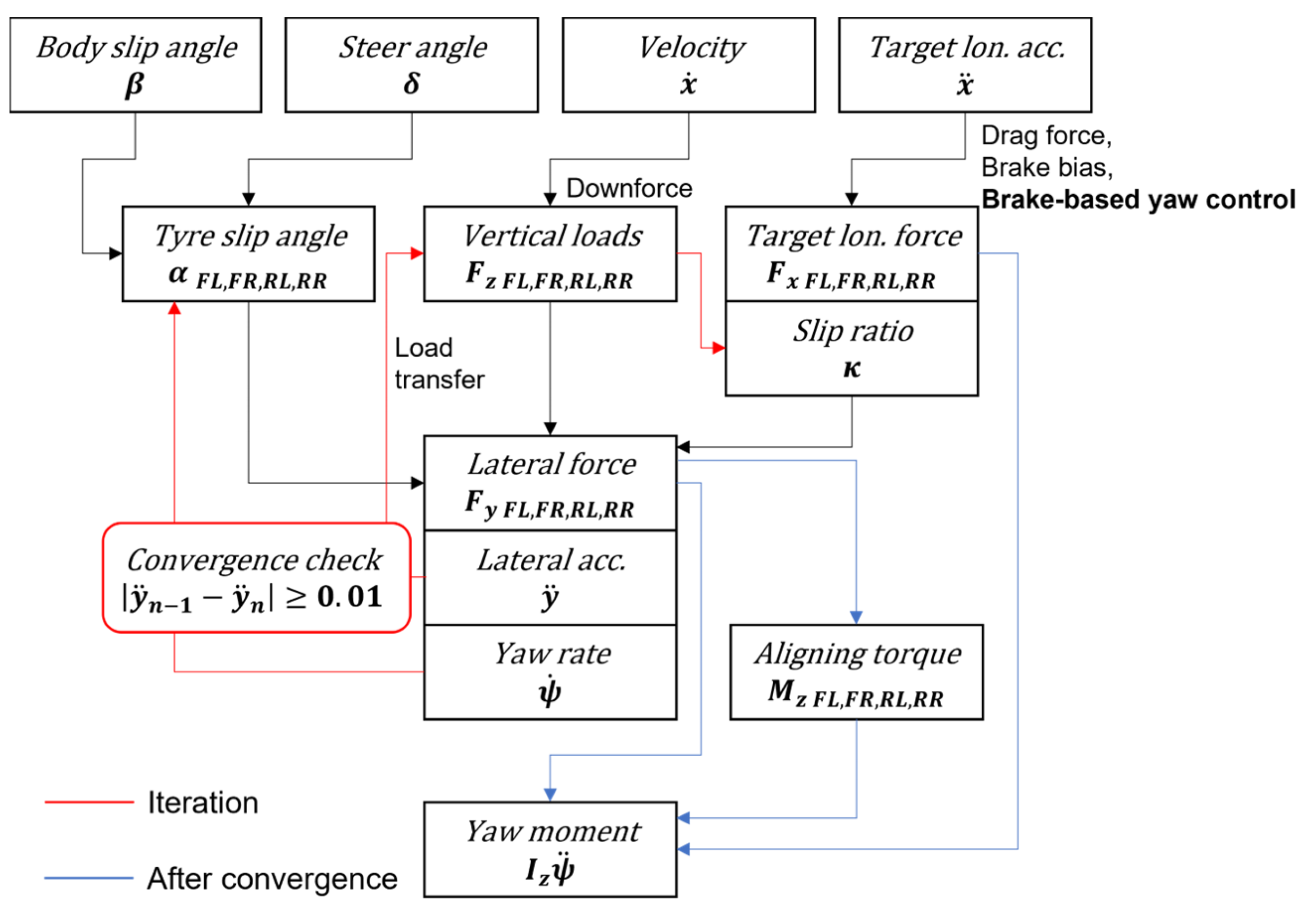
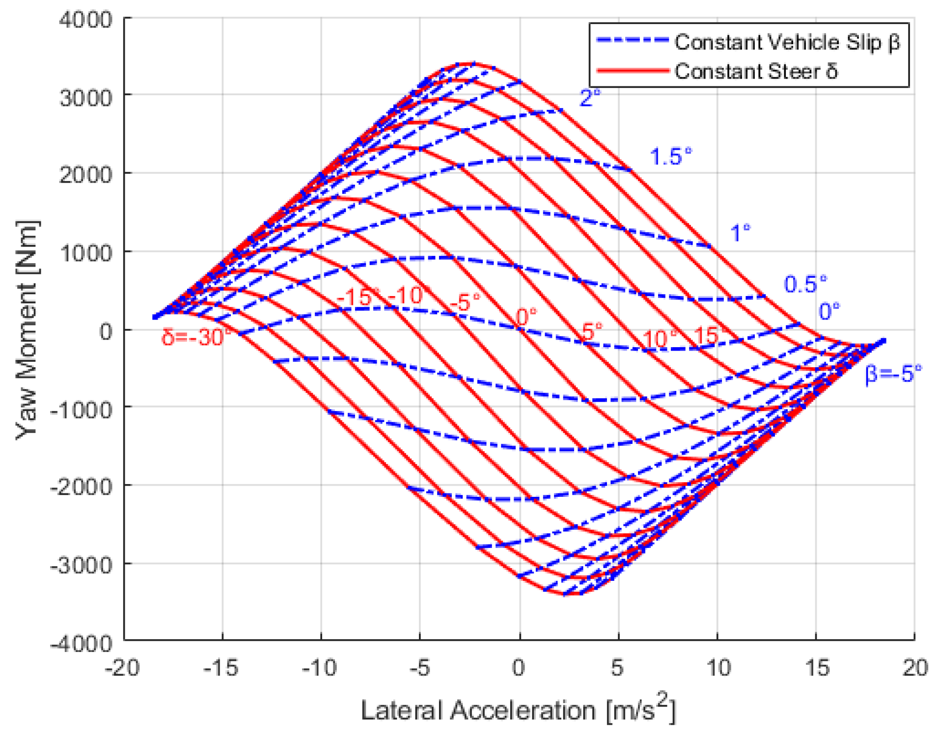
Considering its use in circuit driving, a system that uses brake torque to control the yaw moment must consider optimal brake and powertrain operations, since its characteristics may reduce vehicle speed, which may lead to a deterioration in lap times. Since it is not realistic to consider many experimental studies, simulation is expected to be used. However, most of the yaw moment control research cases focused on transient motion characteristics for time-based steering inputs, using full vehicle dynamics simulations, which are widely used in commercial applications. While these full vehicle dynamics simulation-based studies can reproduce realistic behavior, they have the disadvantage of making it difficult to identify the causes and remedies for phenomena caused by complex and continuous effects, which can hinder progress in development. The forces and moments acting on a vehicle during a turn can be well understood using the Milliken Research Associates (MRA) moment method [13], a quasi-steady-state vehicle maneuvering representation. The Milliken moment method (MMM) is a simulation technique similar to the restricted condition test method used in aircraft wind tunnel testing, where the yaw direction motion is constrained. By calculating the steady-state cornering forces and yaw moment at that time using a combination of the vehicle slip angle and steering angle as inputs, analyzing the orbital and spinning motion performance, stability, and control at any vehicle slip angle and steering angle is possible [14,15,16,17,18]. Compared to transient simulation, quasi-steady simulation is suitable for the development of yaw moment control because it allows the driver’s input regarding handling and the output from the vehicle, i.e., lateral acceleration and yaw moment, to be understood in a single diagram. In addition, there has been no application of this method to the development of yaw moment control for race cars, and we expect that this method will be used as a new study method for yaw moment control through this research.
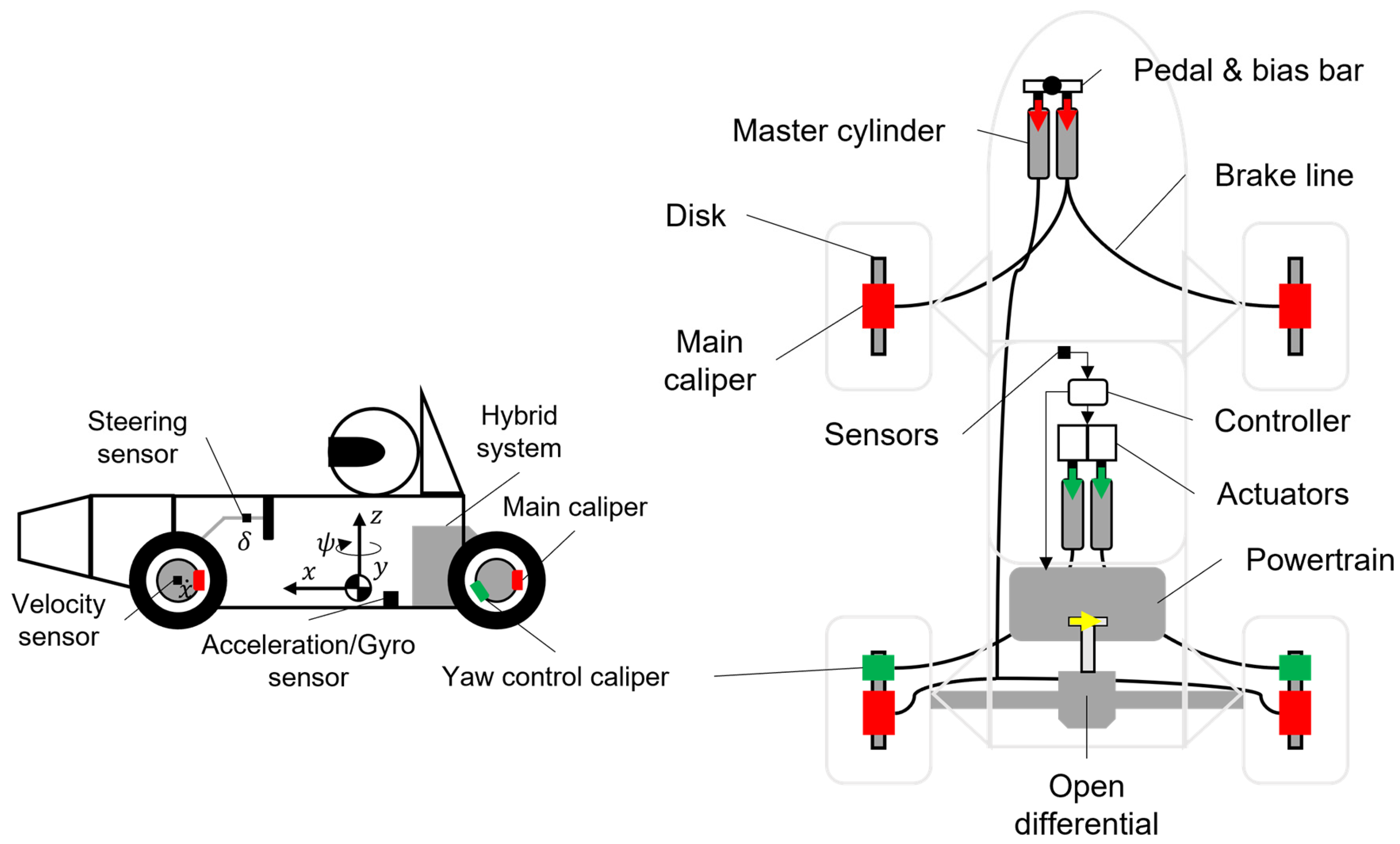
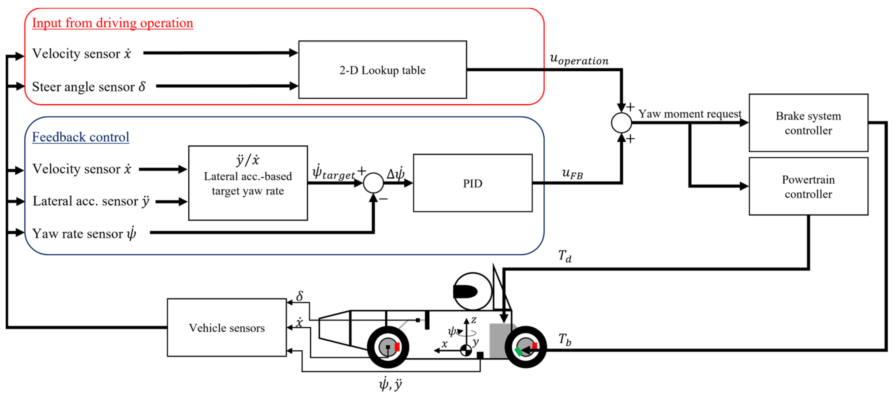
I. Kobayashi studied hybrid race cars using an internal combustion engine (ICE) and an electric motor and proposed a system that varies the output of the ICE and electric motor, depending on vehicle conditions [19,20,21]. In this study, we used the vehicle dynamics model that we previously developed. We proposed a yaw moment control technique that actively utilized drive torque and brake torque. These could be applied to many vehicles, including internal combustion engines, as well as the hybrid competition vehicles we are studying. We compared the performance of the vehicle with and without the proposed system using the MRA moment in quasi-steady-state conditions, based on the nonlinear Magic Formula 6.1.2 tire [22] and two-track models. We undertook the performance verification of lateral acceleration and yaw moment using the method and a comparison of the vehicle with and without the proposed system, in terms of time and performance, using variable corner radius simulation while assuming circuit driving.

2. Proposed Yaw Moment Control System

2.1. Outline of the Proposed System

The yaw moment I z ψ ¨ , which is the main control target in the proposed yaw moment control system proposed herein, is determined by three factors: longitudinal force F x , lateral force F y , and self-aligning torque M z for each of the four tires. The three factors, vehicle’s longitudinal weight distribution w d f , wheelbase w b , and front/rear track width t f , r represent the function contained in Equation (1), where I z is the yaw inertia of the vehicle, and ψ ¨ is the yaw angular acceleration.
I z ψ ¨ = f n F x , F y , M z , w d f , w b , t f , r
The proposed yaw moment control system using a powertrain and a brake system is shown in Figure 2 and Figure 3. This system is a simple mechanism that adds a conventional hydraulic brake system to the two rear wheels (green) and uses actuators instead of pedals to achieve active control. Brakes generated by the pedals (red) function in the same way as in a normal car. Figure 4 shows an image of an actual operational system. These actuators generate force on either side in response to yaw moment demands, and the controller determines the amount of control based on information from vehicle-mounted sensors. As the generation of brake force F b (green arrows) causes acceleration in the negative direction, simultaneously, the drive torque T d (yellow allow) of the powertrain system is placed at the wheel position and increased by the same amount as the brake torque T b to generate driving force F d on the opposite side of the rear tire. The yaw moment Δ I z ψ ¨ added at the vehicle’s center of gravity position by the rear tire track width t r is given by Equation (2).
Δ I z ψ ¨ = 0.5 t r F d F b
From the above system configuration, the relation between the added driving force and the braking force is given by Equation (3).
F e m = F d

2.2. Control Algorithm

The algorithm for this yaw moment control system is shown in Figure 5. The amount of yaw moment required is calculated by two algorithms, based on the control quantity u o p e r a t i o n determined by a 2D lookup table from the driver’s operations, that is, steering operation δ and vehicle speed x ˙ , and the control quantity u F B is determined by the PID control that eliminates the deviation of the actual yaw rate ψ ˙ from the target yaw rate ψ ˙ t a r g e t , based on the lateral acceleration y ¨ . Once the yaw moment is determined, the brake system controller and powertrain controller (ECU) are signaled with the required torque, and the vehicle generates brake torque and drive torque.
The control quantities u F B determined by the PID control in this algorithm are the actions that place the vehicle in a neutral state. This can be explained by the basic vehicle motion equations shown in Equation (4) and Figure 6.
y ¨ = V ˙ y + ψ ˙ V x
where y ¨ is the lateral acceleration, V ˙ y the time derivative of the lateral velocity component, ψ ˙ is the yaw rate, and V x is the longitudinal velocity. The time derivative of the lateral velocity component can be simplified, as shown in Equation (5), because the lateral slip angle of the vehicle body is dominant, and its magnitude is minute.
y ¨ ψ ˙ V x
Given the corner radius R , we can obtain the relation in Equations (6) and (7).
ψ ˙ = V x R = y ¨ V x
y ¨ = ψ ˙ V x = V x 2 R
The calculation shown in Equation (6) is the yaw rate at which the vehicle body rotates in accordance with the traveling trajectory, which can be defined as the neutral state target yaw rate ψ ˙ t a r g e t . This is the formula for deriving the yaw rate during a steady-state turning. In other words, the system works with the yaw moment to follow the yaw rate determined from the orbital motion performance. For the driver operation-derived control quantity u o p e r a t i o n , we used the 2D lookup table shown in Figure 7. These directly specify the actual yaw moment to be added as the output and can be set according to various conditions, such as driver, circuit, and weather.
By combining these two algorithms, creating a 2D lookup table for the conditions of a vehicle that always produces a neutral state is possible. From the aforementioned algorithm, the amount of yaw moment to be added can be set. However, because the drive torque needs to be equal to the brake torque around the wheels, the formula in Equation (2) must be used to ensure that the output performance of the powertrain is not exceeded if a large yaw moment is to be added.
In practice, the slip ratio is dominant in the magnitude of the longitudinal force on the tire. Therefore, dynamically controlling the torque to the slip ratio state required from the required yaw moment is necessary. In this study, Equation (8) and the assumptions shown in Figure 8 were used to deal with motion in a quasi-steady state.
T F x r t
where T denotes the torque around the wheel, F x denotes the longitudinal force at the tire contact patch, and r t denotes the tire radius.

3. Calculation Method using Milliken Moment Diagram

3.1. Vehicle Dynamics Model

The equations of planar and rotational motions of the vehicle were calculated by considering the forces in the x–y direction at the center of gravity and the moment around the z-axis, with four tire front/rear forces F x , lateral forces F y , and self-aligning torque M z . The steering angle δ , front/rear track width t f , r , and distance l f , r from the center of gravity to the front and rear tire contact patches were also used in the calculations. Figure 9 and Equations (9)–(11) show the equations of the planar and rotational motion dynamics of the vehicle. The effects of the vehicle body slip angle and yaw rate on the longitudinal and lateral accelerations were neglected.
m x ¨ = c o s δ F x F L + F x F R + F x R L + F x R R s i n δ F y F L + F y F R
m y ¨ = c o s δ F y F L + F y F R + F y R L + F y R R + s i n δ ( F x F L + F x F R )
I z ψ ¨ = l f c o s δ F y F L + F y F R + s i n δ F x F L + F x F R l r F y R L + F y R R + 0.5 t f c o s δ F x F L F x F R s i n δ F y F L F y F R + 0.5 t r F x R L F x R R M z F L M z F R M z R L M z R R
For the vertical load, the static load F z S , downforce F z D F , and load transfer Δ F z were considered, and the vehicle speed x ˙ and longitudinal and lateral accelerations x ¨ and y ¨ were affected. Equations (12) and (13) show the calculation of the vertical load F z S F , R on a longitudinal wheel under static conditions. The mass of the vehicle is stated in m , the weight distribution on the front side in w d f , and the gravitational acceleration in g .
F z S F = m g w d f 2
F z S R = m g 1 w d f 2
The downforce F z D F F , R applied to the four wheels was calculated using Equations (14) and (15). The following equations were used for air density ρ , frontal area A , lift coefficient C L , and downforce distribution a d f . The lift coefficient and downforce distribution were modeled as constants.
F z D F F = 0.5 C L A ρ x ˙ 2 a d f
F z D F R = 0.5 C L A ρ x ˙ 2 ( 1 a d f )
The load transfer was calculated using the total mass m and the total center of gravity height h C o G , without separating the mass above the springs and the mass below the springs. In addition, as there was no need to focus on transient load transfer for the analysis of motion in a quasi-steady state, load transfer through the springs and load transfer through the suspension links in the aforementioned spring mass were not separately calculated. Simultaneously, the influence of damping was neglected. The lateral load transfer Δ F z L a t F , R was calculated using Equations (17) and (18). As shown in Equation (16), the same values were used for the front and rear track widths, and the modeling was performed by specifying the value of the total lateral load transfer distribution T L L T D , occupied by the front wheels, with respect to the front–rear distribution of the lateral load transfer. The longitudinal load transfer Δ F z l o n was calculated using Equation (19), where w b denotes the wheelbase.
t m = t f = t r
Δ F z L a t F = m y ¨ h C o G t m T L L T D
Δ F z L a t R = m y ¨ h C o G t m ( 1 T L L T D )
Δ F z L o n = m x ¨ h C o G 2 w b
The final vertical load, F z , which is the sum of the load variation factors, was calculated using Equations (20)–(23). The vertical load at each of the four wheels was calculated to influence the tire model, as described below.
F z F L = F z S F + F z D F F 2 + Δ F z L a t F Δ F z L o n
F z F R = F z S F + F z D F F 2 Δ F z L a t F Δ F z L o n
F z R L = F z S R + F z D F R 2 + Δ F z L a t R + Δ F z L o n
F z R R = F z S R + F z D F R 2 Δ F z L a t R + Δ F z L o n
The calculation of slip angle α for each tire is shown in Figure 10 and Equations (24)–(27). The yaw rate ψ ˙ , representing the slip angle β and steering angle δ of the vehicle, and the relation between the tire position and center of gravity position affected the longitudinal and lateral velocity components, V x , y , for each tire contact patch.
α F L = V y + ψ ˙ · l f V x + ψ ˙ · t f / 2 δ
α F R = V y + ψ ˙ · l f V x ψ ˙ · t f / 2 δ  
α R L = V y ψ ˙ · l r V x + ψ ˙ · t r / 2
α R R = V y ψ ˙ · l r V x ψ ˙ · t r / 2

3.2. Tire Model

The semi-experimental identification tire model Magic Formula 6.1.2 was used to represent the nonlinear characteristics of longitudinal force F x , lateral force F y , and self-aligning torque M z . Based on tire test data, we identified 130 parameters in the tire model equations. Equation (28) shows the inputs and outputs of the model. This model was a steady-state tire model, where forces and moments were determined by the inputs of vertical load F z , slip angle α , inclination angle γ , slip ratio κ , internal pressure p , and rolling speed v x . Parameters were included in the tire model equations to relate them to these inputs. It did not consider the effects of onset delay and relaxation length.
F x , F y , M z = f n F z , α , γ , κ , p , v x
After modeling the pure slip equation representing the longitudinal force F x 0 when the tire slip angle was set to zero and the lateral force F y 0 when the tire slip ratio was set to zero, the pure slip condition was normalized such that its weight was 1. This equation was then used as the combined slip equation. By fitting the concavo-convex shape with a weighting function, calculating the conditions for the slip angle and slip ratio to simultaneously occur was possible. Figure 11 shows the surface of the weighting functions G x α and G y κ . The calculation of the longitudinal force F x and lateral force F y are shown in Equations (29) and (30), respectively.
F x = F x 0 G x α
F y = F y 0 G y κ

3.3. Milliken Moment Diagram Calculation Method

To create the Milliken moment diagram (MMD), the vehicle body slip angle β , steering angle δ , speed x ˙ , and target longitudinal acceleration x ¨ were given, as shown in Figure 12, where the lateral forces were first calculated using the static vertical loads and downforce. The process was iterated until the lateral acceleration converged to the specified criteria. This is because the load transfer is a function of acceleration, and comparing the acceleration used in the load transfer with the calculated acceleration is necessary. Simultaneously, the ideal yaw rate was calculated by dividing the lateral acceleration by the speed, which affected the tire slip angle. To apply the combined slip condition, which included the tire longitudinal force and slip ratio, the drag force, brake bias, brake force, and drive force of the system were used to determine the target longitudinal force and slip ratio for each of the four wheels to influence the lateral force. After the convergence of lateral acceleration, the self-aligning torque and yaw moment were calculated.
These series of calculation flows were used to create the MMD shown in Figure 13. All the conditions from the set combination of the vehicle slip angle and steering angle were calculated, and the constant steering angle line and constant vehicle slip angle line at each plot point were drawn. In this study, the MMD was expressed using the units and definitions of the lateral acceleration [m/s2] and yaw moment [Nm].
MMD is useful for visually understanding the cornering process, which includes the vehicle’s spinning and orbital motions; however, it is more effective when the point of focus is specified. As shown in Figure 14, the maximum lateral acceleration on the diagram indicates the limit of the vehicle, whereas the yaw moment indicates the yaw balance of the vehicle at the limit cornering. The maximum lateral acceleration on the line of the zero-yaw moment indicates the limit performance of the constant-radius turning (skid pan) condition. The controllability of the yaw moment during corner entry was calculated using Equation (31). In this report, we focused on the amount of change in the yaw moment when the vehicle body slip angle and steering angle varied from zero to the steering angle. The controllability of the vehicle was negative for the MMD under low-velocity conditions. This is because the yaw rate is larger at low speeds; therefore, the degree of control that determines the tire slip angle is dominated by the yaw rate.
C o n t r o l l a b i l i t y = Δ I z ψ ¨ Δ δ

4. Performance Prediction of Proposed Yaw Moment Control Systems

4.1. Analysis Conditions

To verify the improvement in the vehicle dynamic performance with the proposed yaw moment control system, two MMD-based analyses were used to compare it with the performance of a vehicle not equipped with the proposed system.
First, a comparison was made focusing on the maximum lateral acceleration using MMD, the yaw moment at the point of maximum lateral acceleration, the maximum lateral acceleration during the steady state, and the change in yaw moment per steering angle, assuming the entry of turning.
Second, a vehicle performance envelope was created using the MMD to calculate the time on the variable turning radius track, where the corner radius became increasingly smaller, assuming a situation where the yaw moment was required, and to verify the improvement in vehicle performance when the vehicle was driven at the limit.
The parameters of the vehicle model used in the analysis are listed in Table 1. The base model targets Formula SAE, a global competition where students design and build race cars to compete in terms of performance. The tire model responds to changes in internal pressure and camber angle; however, in this study, the internal pressure and camber angle were fixed at 82.75 kPa and 0°, respectively, to focus only on the improvement of vehicle performance by the proposed system. Simultaneously, dynamic toe changes were not considered.

4.2. Comparison by Milliken Moment Diagram

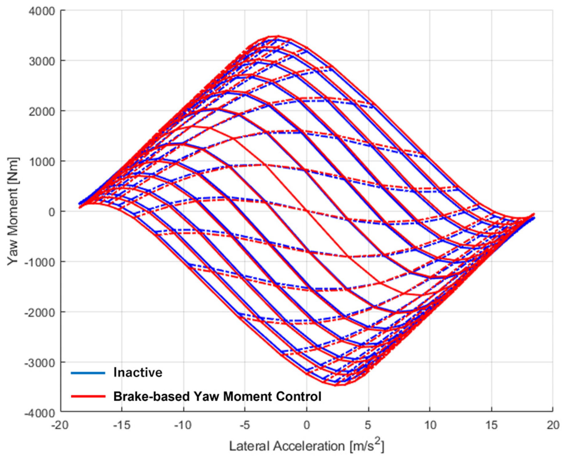
First, a comparison was made with vehicles not equipped with the proposed system using MMD. In this analysis, the conditions were fixed at a vehicle velocity of 15 m/s and a longitudinal acceleration of 0 m/s2. The velocity was the average velocity of the subject vehicle on the race track, and the longitudinal acceleration of zero was a condition in which the driving force was actually applied to the rear tires, due to the generation of the drag force.
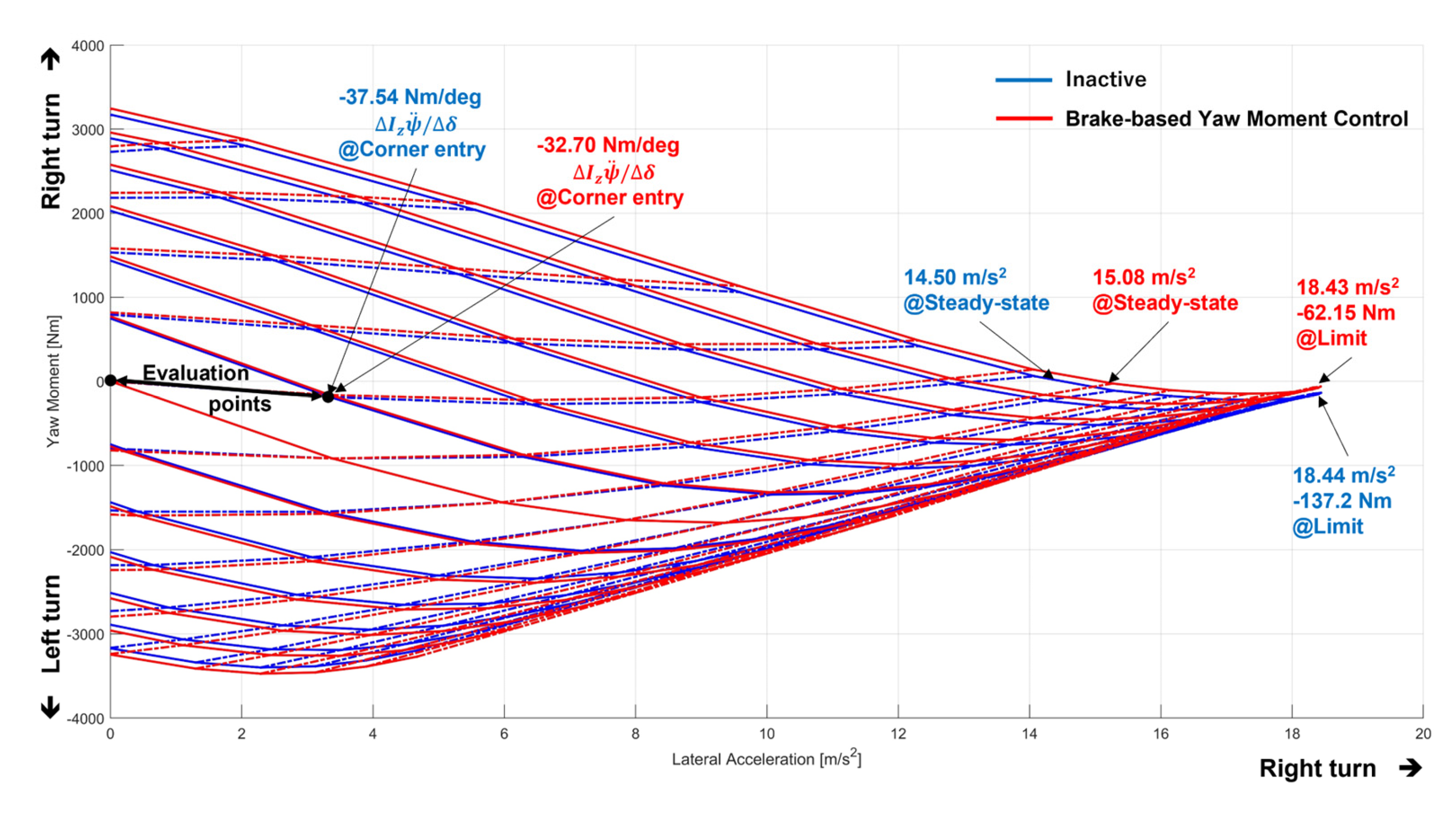
In the MMD of Figure 15, the entire diagram extended in the Y-axis direction, and the vehicles equipped with the proposed system, represented by the red line, showed an improvement in yaw moment, compared to the vehicles without the system, represented by the blue line, for all combinations of steering angle and vehicle slip angle. Additionally, there was no significant decrease in lateral acceleration. It was also confirmed that the characteristics of the control algorithm of this system did not change the vehicle characteristics, as the system was not activated at a constant line with a steering angle of 0°.
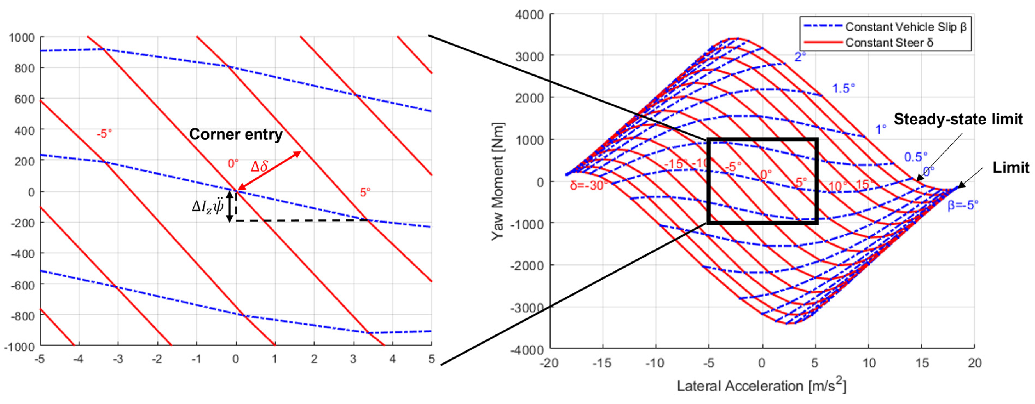
Figure 16 and Table 2 show the comparison results of vehicle performance with and without the proposed system at each evaluation point in the right-turn situation, with positive lateral acceleration for the MMD in Figure 15, along with numerical values.
First, for the maximum lateral acceleration, assuming the apex of the corner, the yaw moment at the maximum lateral acceleration was 18.43 m/s2 for the vehicle equipped with the system and 18.44 m/s2 for the vehicle without the system; although there was no significant difference, the proposed system had about a 75 Nm larger yaw moment at the maximum lateral acceleration, confirming that the vehicle’s spinning performance was improved without degrading the orbital motion performance. The performance improvement of 0.58 m/s2 was also confirmed for the lateral acceleration under the steady-state turn radius condition with zero yaw moment. This was because the basic characteristics of the baseline vehicle were on the under-yaw moment side, and the vehicle equipped with the system was able to generate higher lateral acceleration, due to the increased yaw moment. The change in yaw moment when the steering angle of the steering wheel position was changed from 0° to 5°, simulating a scenario in the early stages of a corner, also showed an increase in value of about 5 Nm/deg for the system-equipped vehicle, confirming improved controllability in situations where the need for yaw moment in the early stages of a turn is high.
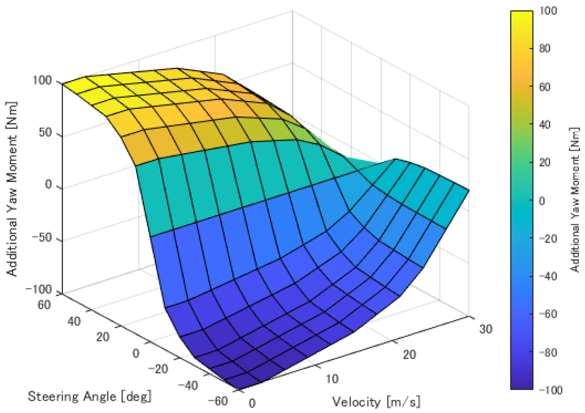
The evaluation of MMD analysis in the above four points showed that vehicles equipped with the proposed system improved yaw moment without significantly reducing lateral acceleration. These improvements in self-spinning performance have the potential to improve vehicle performance, especially on circuits with high yaw motion requirements, such as a series of tight corners. However, the rate of increase in yaw moment of the vehicle equipped with the proposed system relative to the vehicle without the system was higher near the apex of the corner than at the beginning of the turn; this was largely due to the setting of the 2D lookup table determined by the steering angle and speed in the control algorithm. In this study, the amount of additional yaw moment around the small steering angle was set to be small. In actual situations, the required yaw moment differs at each point of a corner, so it is necessary to set the required amount of yaw moment based on an understanding of the yaw moment.

4.3. Comparison by Variable Turning Radius Simulation

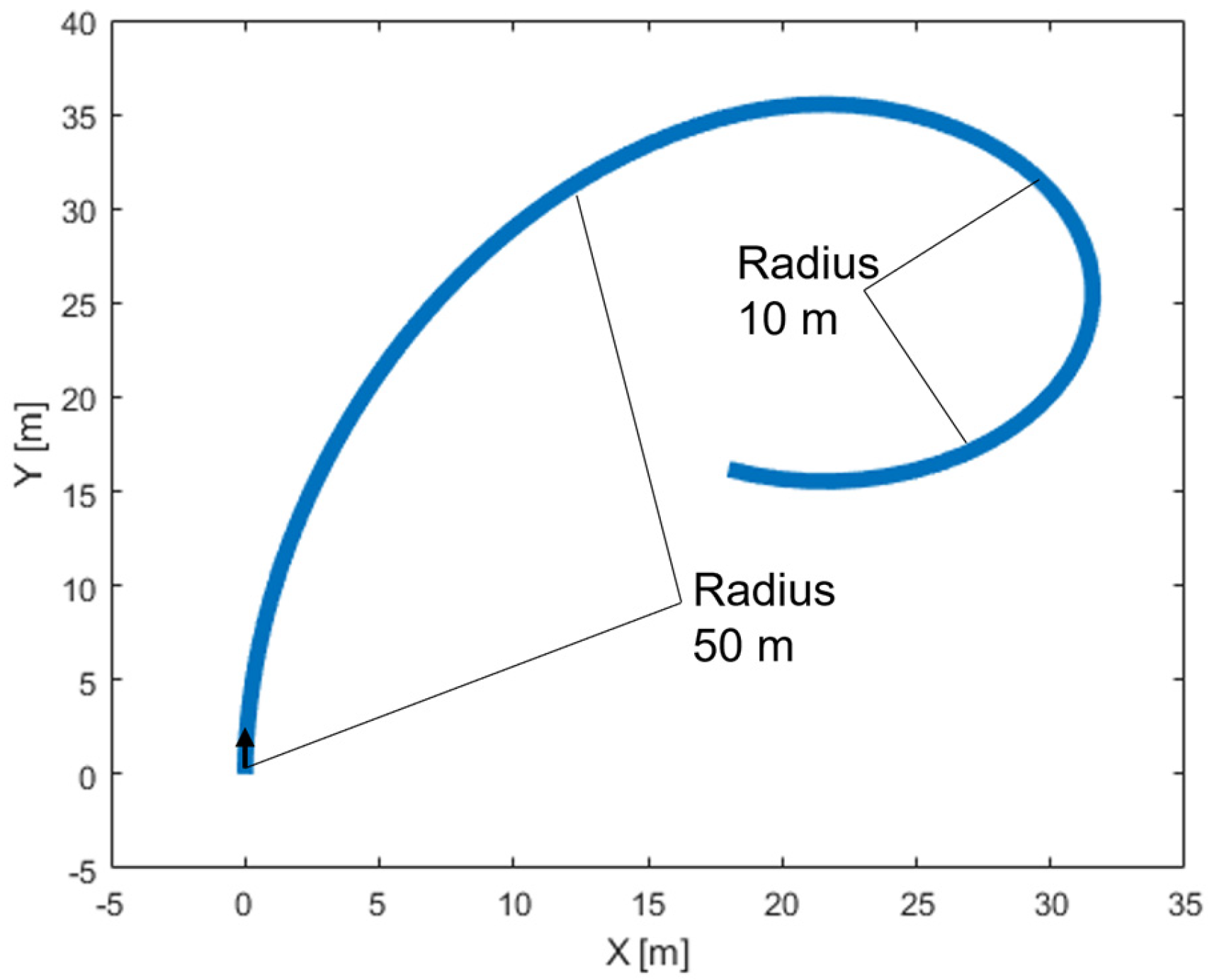
The performance of the vehicle equipped with the proposed system was verified when the vehicle was driven on a variable turning radius track that actually required a yaw moment. The evaluation track was an 80 m long track, whose turning radius decreased from 50 m to 10 m, as shown in Figure 17.
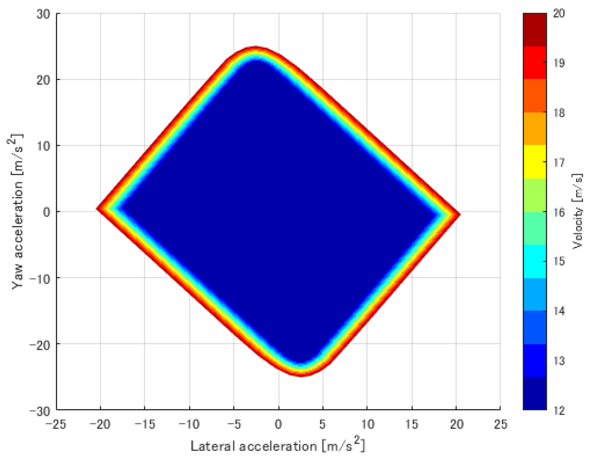
The vehicle performance envelope, shown in 
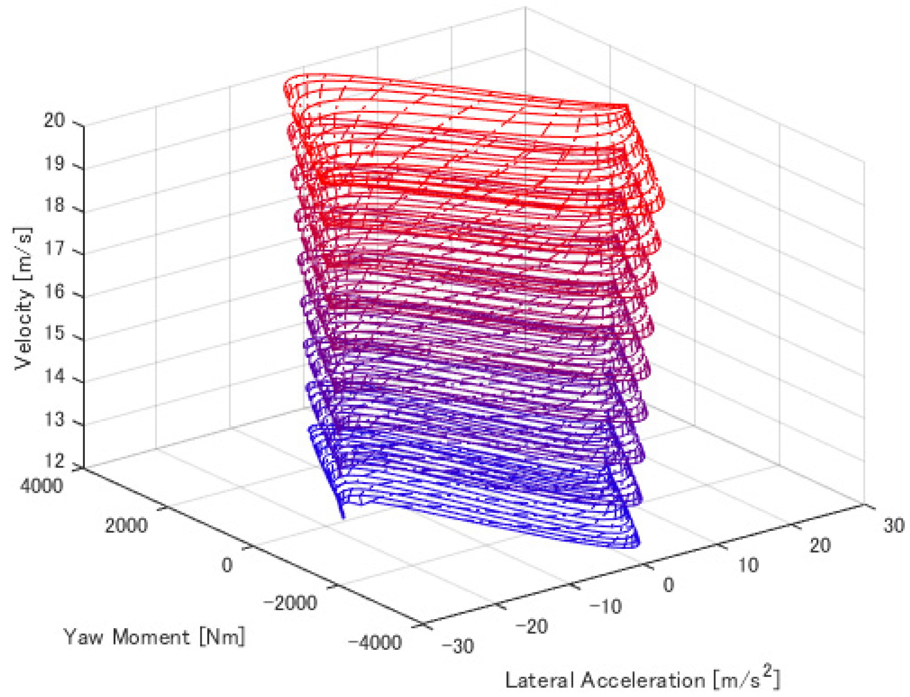
Figure 18, was created to simulate the driving of this evaluation track at its limits. The purpose of this was to deal with velocity-dependent vehicle performance, including downforce. As shown in Figure 19, creating vehicle performance charts for yaw acceleration, lateral acceleration, and velocity by creating an MMD for each velocity and subsequently creating a 3D envelope was possible. The color of the lines in the figure indicates the difference in velocity, calculated from 12 to 20 m/s. In the case of acceleration/deceleration, longitudinal acceleration should also be considered in the performance envelope. However, in this study, a performance envelope was created with zero longitudinal acceleration to verify the turning performance, including rotation and revolution.
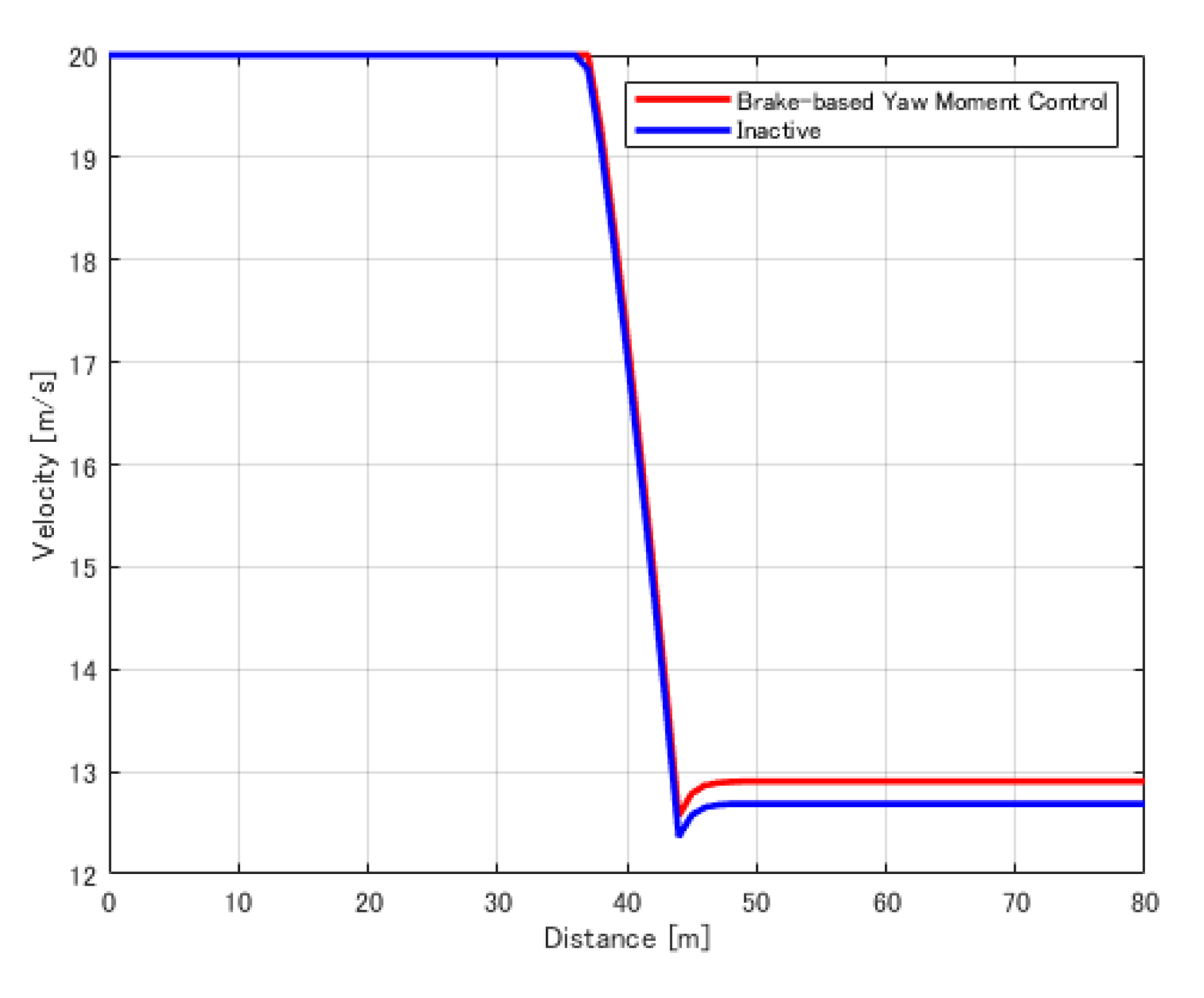
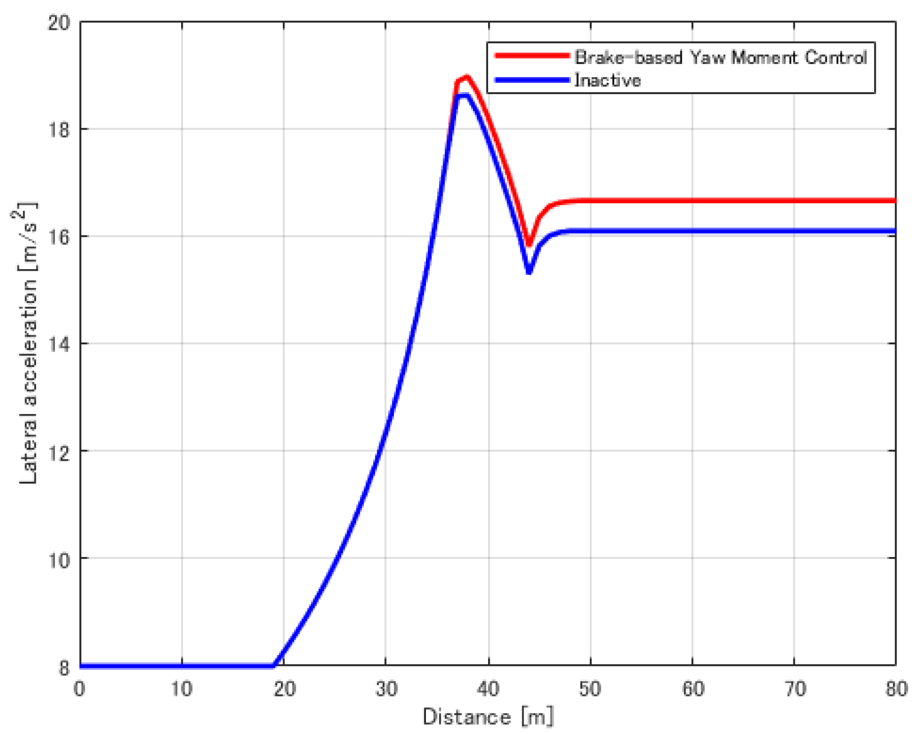
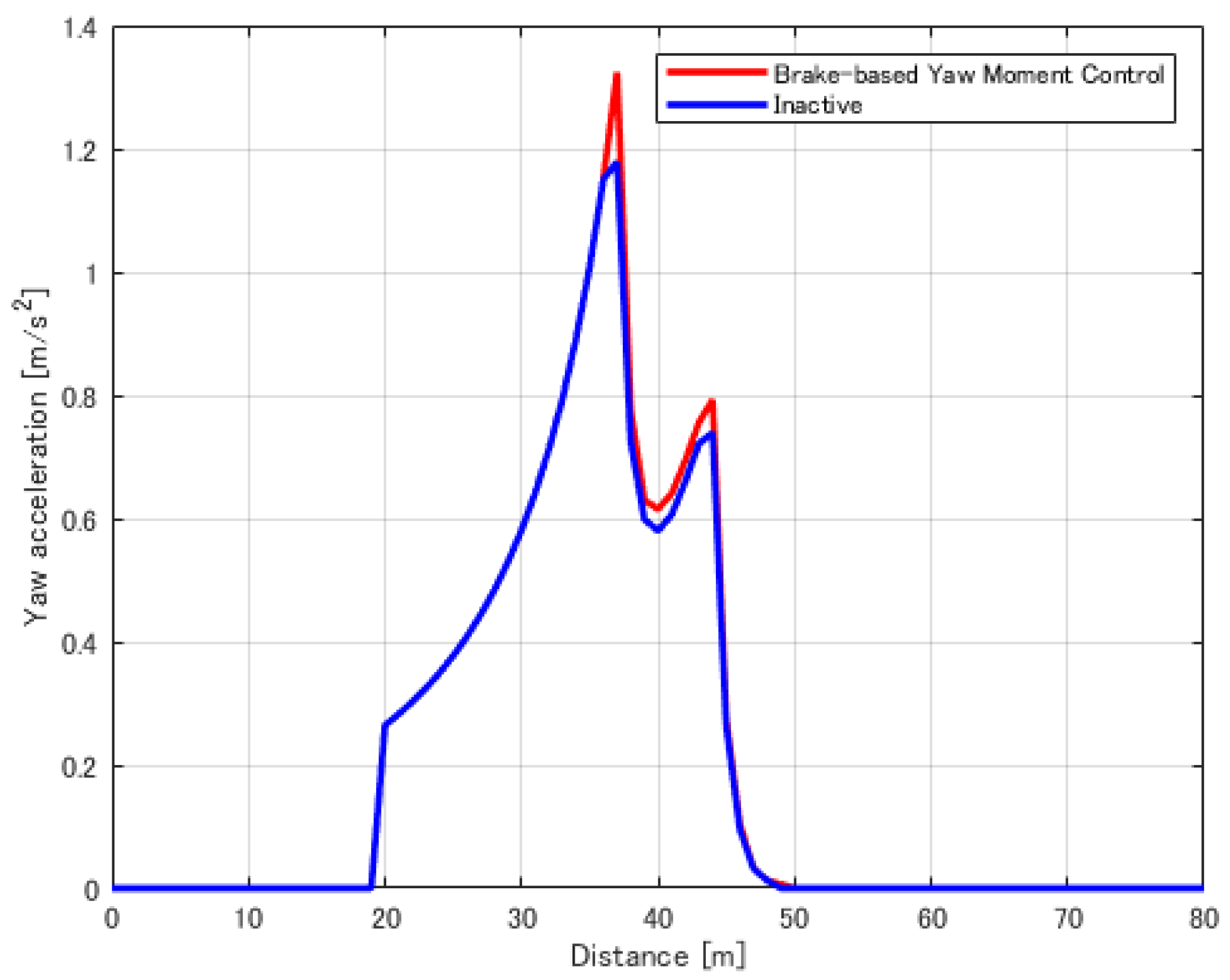
Comparison logs between vehicles equipped with the proposed yaw moment control system and inactively controlled vehicles are shown in Figure 20, Figure 21, Figure 22 and Figure 23 when the vehicles entered the evaluation track at an initial speed of 20 m/s and ran within this vehicle performance envelope. Figure 20 shows that the vehicle equipped with the proposed system had a higher velocity in all areas than the inactive vehicle. Figure 21 shows that the yaw moment at the performance limit approached zero by the proposed system because the basic characteristic of the vehicle model was the yaw moment, as mentioned above, and thus, the vehicle benefited from the improvement in steady-state lateral acceleration. However, the proposed system was the most effective in the area where the most yaw moment was generated, as shown in Figure 22 and Figure 23. The proposed system met the demand for higher yaw moment, due to the higher turning speed.
The transit times of the vehicles equipped with the proposed yaw moment control system and the inactive control vehicle on this evaluation track are listed in Table 3. The times improved, due to the improvement in lateral acceleration in the steady state and the improvement in performance in the area where considerable yaw moment was required.
Since the focus of this consideration was to evaluate the behavior of the proposed system in quasi-steady-state conditions, the vehicle performance diagram and system controls used to analyze the vehicle running a variable radius used only lateral and yaw accelerations in the quasi-steady state. Future work will examine elements that include transient conditions, such as the evaluation of controls that bring the constantly dynamic yaw rate closer to a target yaw rate calculated from the steady-state turning formula and the evaluation of times in circuit driving, using a multi-body full vehicle dynamics model. In addition, since the maximum yaw moment that can be added to this system ultimately depends on the driving force limit of each tire, it is necessary to consider vertical loading, which has a high contribution to tire performance. Therefore, transient lateral and longitudinal load transfer using a full vehicle dynamics model will also be considered in the future.

5. Conclusions

In this study, we presented the system configuration, control algorithm, and theory as preliminary research of the proposed yaw moment control system. This study also confirmed the improvement of the vehicle motion performance of the proposed system by analyzing the vehicle motion using the MMM technique, effectively showing the vehicle’s spinning and orbiting motion performance in a quasi-steady state. The improvement in the self-spinning motion performance of the proposed system was confirmed. Furthermore, the analysis using a variable turning radius track designed as a race track not only enabled a comparison focused on the performance, particularly during corner radius entry, it also demonstrated the usefulness of this variable turning radius study method.
In the future, we plan to conduct a motion analysis that considers longitudinal acceleration, which was not considered in this study, and the performance of the vehicle on a single lap of a race track. In addition, studying the transient motion characteristics, which are indispensable for the construction of a control system for implementation, is necessary.

Author Contributions

Conceptualization, I.K.; methodology, I.K. and H.K.; software, I.K.; validation, J.K., D.U. and A.E.; formal analysis, I.K.; investigation, K.O.; resources, T.N.; data curation, H.K.; writing—original draft preparation, I.K.; writing—review and editing, M.H.B.P. and T.N.; visualization, K.I. and T.K.; supervision, H.K.; project administration, H.K.; funding acquisition, T.N. All authors have read and agreed to the published version of the manuscript.

Funding

This research received no external funding.

Institutional Review Board Statement

Not applicable.

Informed Consent Statement

Not applicable.

Data Availability Statement

Not applicable.

Conflicts of Interest

The authors declare no conflict of interest.

References

  1. O’Kane, C.; Timoney, S. Investigation of Four-Wheel Steering Algorithms for a Formula SAE Car. In SAE Technical Paper; SAE International: Pittsburgh, PA, USA, 2004. [Google Scholar] [CrossRef] [Green Version]
  2. Chien, P.-C.; Chen, C.-K. Integrated Chassis Control and Control Allocation for All Wheel Drive Electric Cars with Rear Wheel Steering. Electronics 2021, 10, 2885. [Google Scholar] [CrossRef]
  3. Andrzej, D.; Jakub, F. The bicycle model of a 4WS car lateral dynamics for lane change controller. IOP Conf. Ser. Mater. Sci. Eng. 2021, 1247, 012021. [Google Scholar] [CrossRef]
  4. Medina, A.; Bistue, G.; Rubio, A. Comparison of Typical Controllers for Direct Yaw Moment Control Applied on an Electric Race Car. Vehicles 2021, 3, 127–144. [Google Scholar] [CrossRef]
  5. Raksincharoensak, P.; Daisuke, S.; Lidberg, M. Direct Yaw Moment Control for Enhancing Handling Quality of Lightweight Electric Vehicles with Large Load-To-Curb Weight Ratio. Appl. Sci. 2019, 9, 1151. [Google Scholar] [CrossRef] [Green Version]
  6. Antunes, J.; Cardeira, C.; Oliveira, P. Torque Vectoring for a Formula Student Prototype. In ROBOT 2017: Third Iberian Robotics Conference. ROBOT 2017. Advances in Intelligent Systems and Computing; Springer International Publishing: Cham, Switzerland, 2018; Volume 694, pp. 422–433. [Google Scholar] [CrossRef]
  7. Jaafari, S.; Shirazi, K. A comparison on optimal torque vectoring strategies in overall performance enhancement of a passenger car. Proc. Inst. Mech. Eng. Part K J. Multi-Body Dyn. 2016, 230, 4. [Google Scholar] [CrossRef]
  8. Pascale, V.; Lenzo, B.; Farroni, F.; Timpone, F.; Zhang, X. Torque Vectoring Control for Fully Electric SAE Cars. Proceedings of XXIV AIMETA Conference 2019; Springer International Publishing: Cham, Switzerland, 2019; pp. 1075–1083. [Google Scholar] [CrossRef]
  9. Woo, S.; Cha, H.; Yi, K.; Jang, S. Active Differential Control for Improved Handling Performance of Front-Wheel-Drive High-Performance Vehicles. Int. J. Automot. Technol. 2021, 22, 537–546. [Google Scholar] [CrossRef]
  10. Cheli, F.; Pedrinelli, M.; Resta, F.; Zorzutti, A. Development of a Control Strategy for a Semi-Active Differential for a High Performance Vehicle. In SAE Technical Paper; SAE International: Pittsburgh, PA, USA, 2007. [Google Scholar] [CrossRef]
  11. Karthik, P. Integrated Brake Based Torque Vectoring Control of Vehicle Yaw Rate and Side-Slip Angle. Master’s Thesis, University of Pretoria, Hatfield, South Africa, 2018. [Google Scholar]
  12. Kakalis, L.; Zorzutti, A.; Cheli, F.; Travaglio, G. Brake Based Torque Vectoring for Sport Vehicle Performance Improvement. In SAE Technical Paper; SAE International: Pittsburgh, PA, USA, 2008. [Google Scholar] [CrossRef]
  13. Milliken, W.; Milliken, D. Race Car Vehicle Dynamics; Society of Automotive Engineers, Inc.: Warrendale, PA, USA, 1995. [Google Scholar]
  14. Kang, D.; Stein, J.; Hoffman, R.; Louca, L. Implementing the Milliken Moment Method using Controlled Dynamic Simulation. In SAE Technical Paper; SAE International: Pittsburgh, PA, USA, 2005. [Google Scholar] [CrossRef]
  15. Hoffman, R.; Stein, J.; Louka, L.; Huh, K. Using the Milliken Moment Method and dynamic simulation to evaluate vehicle stability and controllability. Int. J. Veh. Des. 2008, 48, 132–148. [Google Scholar] [CrossRef]
  16. Acosta, M.; Kanarachos, S.; Blundell, M. Vehicle Agile Maneuvering: From Rally Drivers to a Finite State Machine Approach. In Proceedings of the 2016 IEEE Symposium Series on Computational Intelligence, SSCI 2016, Athens, Greece, 6–9 December 2016; pp. 1–8. [Google Scholar] [CrossRef] [Green Version]
  17. Patton, C. Development of Vehicle Dynamics Tools for Motorsports. Ph.D. Thesis, Oregon State University, Corvallis, OR, USA, 2013. [Google Scholar]
  18. Szűcs., G.; Bári, G. Generating MMM Diagram for Defining the Safety Margin of Self Driving Cars. In IOP Conference Series: Materials Science and Engineering; IOP Publishing: Bristol, England, 2018; Volume 393, p. 012128. [Google Scholar]
  19. Kobayashi, I.; Ogawa, K.; Uchino, D.; Ikeda, K.; Kato, T.; Endo, A.; Bin Peeie, M.H.; Narita, T.; Kato, H. A Basic Study on Hybrid Systems for Small Race Car to Improve Dynamic Performance Using Lap Time Simulation. Actuators 2022, 11, 173. [Google Scholar] [CrossRef]
  20. Sato, Y.; Narita, T.; Kato, H.; Okamoto, T. Proposal of Power Synthesis Mechanism in Hybrid System for Compact Racing Car: A Fundamental Consideration on Structural Design and Vehicle Movement Performance. Proc. Sch. Eng. Tokai Univ. Ser. E 2018, 43, 31–37. [Google Scholar]
  21. Kobayashi, I.; Ogawa, K.; Uchino, D.; Ikeda, K.; Kato, T.; Endo, A.; Narita, T.; Kato, H. Investigation of Gear Ratios for Hybrid System in Small Race Car Using Lap Time Simulation. IFAC-PapersOnLine 2022, 55, 27. [Google Scholar] [CrossRef]
  22. Pacejka, H. Tire and Vehicle Dynamics, 3rd ed.; Elsevier Ltd.: Oxford, UK, 2012; pp. 176–183. [Google Scholar]
Figure 1. Relation between lateral forces and yaw moments in the cornering process of a race car.
Vehicles 05 00029 g001
Figure 2. Illustration of the proposed yaw moment control system.
Vehicles 05 00029 g002
Figure 3. Image of the proposed yaw moment control system.
Vehicles 05 00029 g003
Figure 4. Yaw-moment generation mechanism.
Vehicles 05 00029 g004
Figure 5. Schematic block diagram of the proposed algorithm.
Vehicles 05 00029 g005
Figure 6. Illustration of basic vehicle dynamics equations of motion.
Vehicles 05 00029 g006
Figure 7. The 2D lookup table applied to the proposed control system.
Vehicles 05 00029 g007
Figure 8. Illustration showing the relation between the drive torque and the longitudinal force around the wheel.
Vehicles 05 00029 g008
Figure 9. Schematic of the planar and rotational dynamics model.
Vehicles 05 00029 g009
Figure 10. Scheme of the two-track slip angle model.
Vehicles 05 00029 g010
Figure 11. Modeled combined slip weighting surface: (a) lateral combined slip; (b) longitudinal combined slip.
Vehicles 05 00029 g011
Figure 12. Flowchart of Milliken moment diagram calculations.
Vehicles 05 00029 g012
Figure 13. MMD example at 15 m/s and 0 m/s2.
Vehicles 05 00029 g013
Figure 14. Explanation of MMD focus points and analysis methods.
Vehicles 05 00029 g014
Figure 15. Comparison of the proposed system and inactive control vehicle by MMD.
Vehicles 05 00029 g015
Figure 16. Comparison of the proposed system and inactive control vehicle focused on MMD evaluation points.
Vehicles 05 00029 g016
Figure 17. Schematic of a variable turning radius track.
Vehicles 05 00029 g017
Figure 18. Vehicle turning performance envelope.
Vehicles 05 00029 g018
Figure 19. The 3D MMD diagrams calculated for each velocity.
Vehicles 05 00029 g019
Figure 20. Comparison of vehicles with and without the proposed system in terms of velocity vs. distance.
Vehicles 05 00029 g020
Figure 21. Comparison of vehicles with and without the proposed system in terms of lateral acceleration vs. distance.
Vehicles 05 00029 g021
Figure 22. Comparison of vehicles with and without the proposed system in terms of yaw angular acceleration vs. distance.
Vehicles 05 00029 g022
Figure 23. Comparison of vehicles with and without the proposed system in terms of lateral acceleration vs. yaw angular acceleration.
Vehicles 05 00029 g023
Table 1. Vehicle models used in this analysis.
Vehicle ParametersValue/Name
Total mass [kg]268
CoG height [mm]270
Weight distribution [%Fr]45
Yaw inertia [kgm2]150
Wheelbase [mm]1530
Front track [mm]1250
Rear track [mm]1250
TLLTD [%Fr]60
Lift coefficient [-]−5
Drag coefficient [-]1
Frontal area [m2]1
Downforce distribution [%Fr]45
Brake balance [%Fr]56
Steer gear ratio [ ° / ° ]5
Tyre@83 kPa, γ   = 0°Hoosier 16 × 7.5–10 R20
Table 2. Comparison of four criteria of focus within MMD.
InactiveProposed System
Max lateral acc. [m/s2]
@Limit
18.4418.43
Yaw moment [Nm]
@Limit
−137.2−62.15
Max lateral acc. [m/s2]
@Steady-state
14.5015.08
Δ Yaw moment [Nm/deg]
@Corner entry
−37.54−32.70
Table 3. Comparison of transit times for the variable turning radius track.
InactiveProposed System
Time [s]5.1405.085
Disclaimer/Publisher’s Note: The statements, opinions and data contained in all publications are solely those of the individual author(s) and contributor(s) and not of MDPI and/or the editor(s). MDPI and/or the editor(s) disclaim responsibility for any injury to people or property resulting from any ideas, methods, instructions or products referred to in the content.

