Abstract
The rapid conversion of conventional powertrain technologies to climate-neutral new energy vehicles requires the ramping of electrification. The popularity of fuel cell electric vehicles with improved fuel economy has raised great attention for many years. Their use of green hydrogen is proposed to be a promising clean way to fill the energy gap and maintain a zero-emission ecosystem. Their complex architecture is influenced by complex multiphysics interactions, driving patterns, and environmental conditions that put a multitude of power requirements and boundary conditions around the vehicle subsystems, including the fuel cell system, the electric motor, battery, and the vehicle itself. Understanding its optimal fuel economy requires a systematic assessment of these interactions. Artificial intelligence-based machine learning methods have been emerging technologies showing great potential for accelerated data analysis and aid in a thorough understanding of complex systems. The present study investigates the fuel economy peaks during an NEDC in fuel cell electric vehicles. An innovative approach combining traditional multiphysics analyses, design of experiments, and machine learning is an effective blend for accelerated data supply and analysis that accurately predicts the fuel consumption peaks in fuel cell electric vehicles. The trained and validated models show very accurate results with less than 1% error.
1. Introduction
Globally, various industry sectors have been taking action to reduce global CO2 emissions. The mobility and transport industry responded to this by focusing on the increased electrification of vehicles that have been known as new energy vehicles. This particularly applies to on-road transport, which is one of the major emission resources [1]. Details about the challenges, technologies, and policies toward these efforts in a broader context were discussed in a previous study [2]. The rapid conversion of conventional powertrain technologies to climate-neutral new energy vehicles requires the electrification ramping of light-duty and heavy-duty vehicles. Electrification in mobility, vehicles, and transportation refers, in general, to the enhanced use of electrical energy and the implication of a multitude of hybrid technologies to aid in successful power generation and transmission, as well as to achieve an efficient vehicle operation. All major electrified vehicle technologies in transportation [3,4,5], such as battery electric vehicles (BEVs) [6,7,8], fuel cell electric vehicles (FCEVs) [9,10,11,12], and fuel cell hybrid electric vehicles (FCHEVs) [13,14,15,16,17] require a source of energy that is followed by some power conditioning, i.e., conversion before the traction occurs. The origin of the energy source defines the lifecycle emissions of the electric vehicle and the link to the mitigation of climate change [12,18,19,20,21,22]. As a result, the mobility and transport sectors have been directed towards the use of electrification governed by clean energy sources [2,23,24,25,26,27,28,29]; therefore, a power to vehicle pathway such as elucidated in Ref. [2] was considered in the current study.
This kind of global view enables a smooth linking among the energy, climate, and transport sectors. The inclusion of hydrogen generation, distribution, and utilisation stages is a useful baseline to comprehend the complex strategic interactions among sectors and various technologies whilst performing engineering studies. If the concept is solely applied to a power-to-vehicle chain assuming that the end-user vehicle is a fuel cell electric vehicle (FCEV or FCV), the landscape can be demonstrated as illustrated in Figure 1.
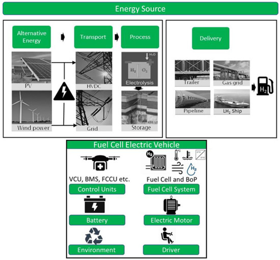
Figure 1.
A landscape from the clean energy source to fuel cell electric vehicle: The electricity generated by clean means is processed via electrolysis to produce green hydrogen and distributed to the fueling station. The fuel cell electric vehicle is a complex system comprising a multitude of constituents.
The main energy source of hydrogen is assumed to originate from regenerative or alternative energy means such as wind power and PV. The generated electricity is transported by grid technologies and can be processed using electrolysis that yields the desired CO2 neutral green hydrogen. Further, the generated hydrogen can be stored in liquid or compressed gas forms or converted to other fluid forms by chemical processes [24,30,31]. Depending on the fluid type and logistic location, the transport of the hydrogen is pursued by methods such as pipelines or existing natural gas infrastructure or displaced in large trailers with marine shipping to be ultimately delivered in smaller amounts and local trailers to the regional fueling stations. Before the hydrogen can be released into the vehicle, its stored pressure is reduced through a pressure valve from high to mid-range, and using a pressure regulator further to the pressure fuel cells can accommodate. Thus far, an understanding of the well-to-tank approach has been recapped.
The fuel cell electric vehicle is a complex system driven by multiphysics interactions. Different driving patterns and environmental conditions put a multitude of power requirements and boundary conditions around the vehicle subsystems, including the fuel cell system, the motor, battery, and the vehicle itself. Each control unit sends and receives signals to yield an efficient operating overall system. The fuel cell system inside the vehicle comprises, in addition to the stack components, auxiliary components, i.e., the so-called Balance of Plant (BoP). This allocates the air, hydrogen, cooling, and power distribution systems. The instantaneous power demand from the driver input is evaluated by the fuel cell control unit and converted to current demand to determine how much current is drawn from the battery versus the fuel cell stack. The local controllers require to translate these signals into a command to define the hydrogen and air requirements. A typical fuel cell vehicle configuration such as the commercially available Hyundai Nexo is illustrated in Figure 2.
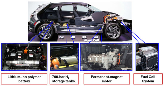
Figure 2.
A typical fuel cell electric vehicle configuration: The Hyundai Nexo is a 135 kW fully dedicated fuel cell electric vehicle (FCEV) platform drawing 95 kW from the fuel cell stack and 40 kW from the 1.56 kW·h, 240-volt lithium-ion polymer battery to operate a 120 kW permanent-magnet motor. Three pieces of 700-bar 52 each H2 storage tanks are used to yield an estimated driving range of 380 miles and an EPA city/hwy/combined MPGe rating of 65/58/61 according to Hyundai.
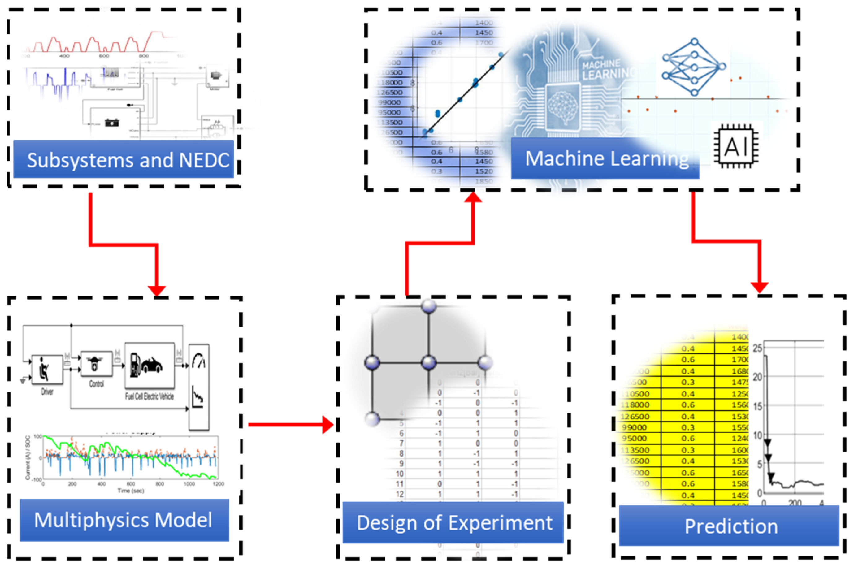
All these systems and components inside the vehicle architecture work together where processes such as thermo-fluid flow, electrochemistry, and thermomechanics are closely coupled. Thus, the external input affects not only the operation of the fuel cell system, but the fuel cell system behaviour itself also influences the powertrain performance. In order to consider these interactions and aid in efficient fuel cell vehicle performance, a thorough understanding of the complex multiphysics is required. In general, multiphysics is described as the science of studying multiple interacting phenomena covering a wide range of physical fields [32]. Numerical methods are the essential platform for predicting the multiphysics behaviour of interacting complex engineering systems [33,34,35,36,37,38,39,40,41,42,43,44]. However, to capture different details and use simulation as a design and optimisation tool, a careful modelling framework needs to be established. There are various methods and workflows within the modelling and simulation field to approach this kind of complex application. First-principles, data-driven statistical methods [45,46,47,48,49,50,51,52] or high-fidelity 3D CFD/FEM multiphysics analyses [53,54,55,56,57,58,59,60] comprising detailed insight into processes, designs, and materials are a few among a bunch of options. The current fuel cell electric vehicles are much more efficient compared to their predecessors. Thus, with increasing fuel efficiency standards, fuel economy or power consumption still remains a major challenge for emerging vehicle technologies. This adds more parameters and complexity to the developed multiphysics models. The handling of these complexities has been improved since numerical methods, software, and hardware computer developments have been progressing. However, the overall modelling workflow has witnessed many significant developments. The present study proposes a systematic combination and effective use of multiphysics simulation, AI-based machine learning, and design of experiments to predict effectively the peaks observed in the fuel consumption behaviour of fuel cell electric vehicles operating under real-life driving conditions. The combined approach is expected to open a perspective for future research in terms of acquisition and handling of big data through sustainable use of the statistical design of experiments, computational multiphysics simulations, and novel predictive tools based on machine learning and AI. The trained model has been an effective tool for pursuing various aspects of fuel cell electric vehicles. The workflow of the systematic approach used in this current study is shown in Figure 3.
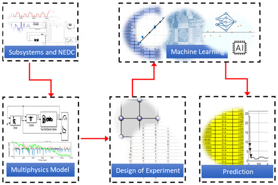
Figure 3.
The used complex workflow: The powertrain component sub-models and driving cycle data are implemented in a full multiphysics model and systematically analysed using DoE. The results are shared with an AI-based machine learning platform to develop, train, and use a tool for accelerated fuel economy predictions.
2. Multiphysics Simulation Methodology
The crucial role of each powertrain component, their interaction, and allocation in the design of the fuel cell electric vehicle system was briefly depicted in the previous section. Investigating and understanding the optimal driving behaviour of a fuel cell electric vehicle requires knowledge about the power consumption and power peaks during driving that contributes to adhering to stringent regulations on fuel economy and a clean environment. The expression optimally used for this kind of complex multiphysics system can be interpreted in such a way that one or more performance features are in an improved state.
However, technically it can be considered a decision-making process, i.e., one selects the appropriate functional option among many other alternatives. The optimised system demands collective intelligence in terms of vehicle configuration and powertrain to be more efficient and to enhance the performance of the overall fuel cell electric vehicle. Even though electric vehicles do not directly burn fuel, they still consume energy, and equivalence measures are applied to predict their performance for comparison purposes and to understand their improvement potential. Thereby, some factors are known to play a more prominent role. The vehicle design configuration, for example, comprising its driving resistance with constituents such as vehicle size and chassis, rolling, and aerodynamic resistance properties or auxiliaries are design factors affecting the energy consumption. In addition to those factors, the powertrain configuration and properties also influence the performance. In fuel cell electric vehicles comprising a storage battery and a fuel cell system to propel an electric motor, several features will particularly be of additional concern. In this section, multiphysics modelling was effectively used to study and understand fuel economy.
2.1. Multiphysics Simulation Model
The used multiphysics model of the fuel cell electric vehicle is presented as a generic dynamic and embedded system model with discrete and continuous time domains running on platforms such as GNU Octave and Scilab. The model has the typical fuel cell electric vehicle constituents, including the powertrain subsystems of PEM fuel cell, Li-Ion Battery storage, electric motor, thermal management, and control units, as well as vehicle properties, driver, and environmental parameters. The fuel cell and battery are linked to the electric motor with an electric network. These attributes are embedded inside block representations covering, for example, inside the driver block the driving cycle data, or in the control block, it covers attributes such as the fuel cell control system, battery management system, brake, and vehicle control unit connections monitoring the vehicle speed, torque limits, etc. The draw ratio between battery and fuel cell is regulated in this way and depicts the recuperation feeding power back into the battery. A simple thermofluid model is used to regulate the temperature of the battery, electric motor, and auxiliaries. The model was used to calculate and estimate the fuel cell and battery current, SOC of battery, and predict the fuel economy in L/100 km while depicting particularly the peaks. The basic model setup is illustrated in Figure 4.
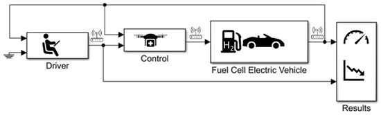
Figure 4.
Employed fuel cell electric vehicle model: The model considers a complex coupled multiphysics architecture comprising parameters of driver, control units, and vehicle. The prediction of interest is fuel economy.
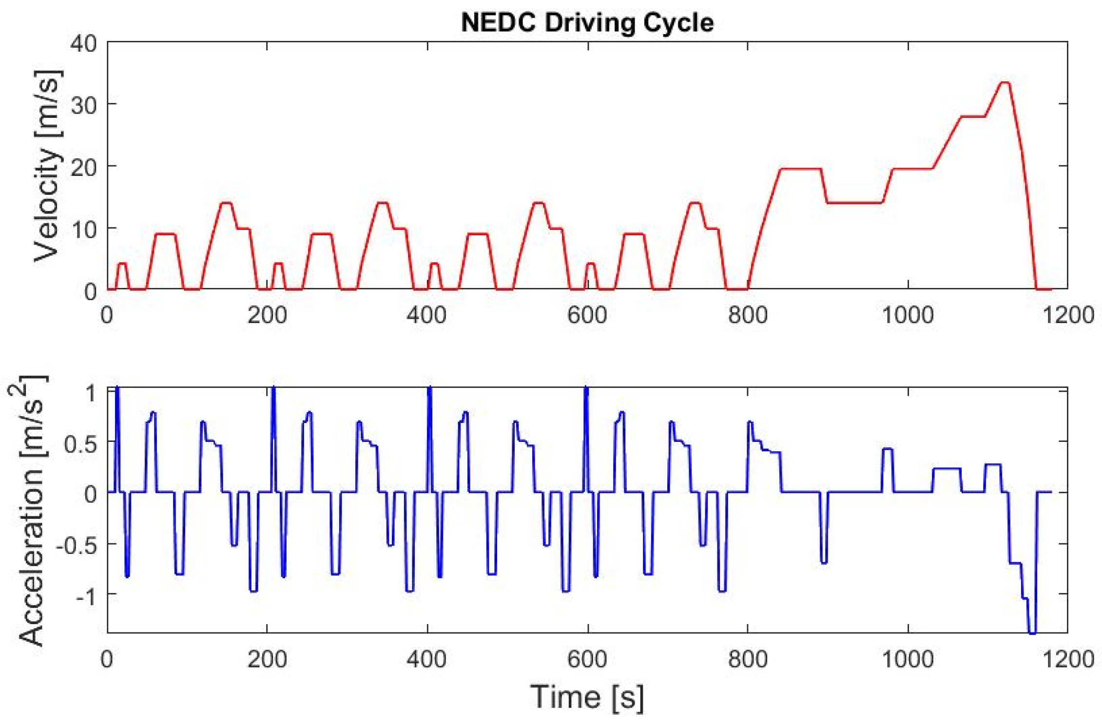
The driving behaviour determined by drive cycles also plays an important role in understanding the fuel economy of vehicles, which is implemented in the model. A standard driving cycle covers a profile of velocity/power-time, which describes the typical driving pattern of a vehicle at a certain region under real-life conditions and is usually tested experimentally on a chassis dynamometer. Typical characteristics such as duration, average, and maximum speed or distance were considered. Currently, the most used standard driving cycles include the New European Driving Cycle (NEDC), China Light-duty vehicle Test Cycle (CLTC), and Urban Dynamometer Driving Schedule (UDDS). The “New European Driving Cycle” (NEDC) [61] is a driving cycle prescribed by the European Union for the typical use of a car in Europe, with measured values for the fuel or power consumption and the driving range of vehicles that enable comparison. From 2017 to 2018, the WLTP (Worldwide harmonized Light vehicles Test Procedure) was the successor of the NEDC. However, EU fleet consumption limits have been related to the NEDC since 2020; thus, the present study considers the NEDC as a driving cycle for simulating the fuel economy and peaks of the employed fuel cell electric vehicle model. The cycle considers basically four urban driving cycles repeated without interruption, aiming to represent low vehicle speed and engine loads reaching a maximum of 50 km/h. The duration of this part lasts for 4 × 195 s, resulting in a total of 780 s and a 4054 km distance. This is followed by a more aggressive extra-urban driving segment to mimic high-speed driving modes reaching a maximum of 120 km/h, equivalent to 33.3 m/s. This segment lasts around 400 s and refers to 6955 km. The average speed for the first four segments reaches approximately 18.7 km/h, whereas the more aggressive last segment approaches 400 s and reaches an average speed of around 62.6 km/h. The implemented driving cycle curves that consider the speed and equivalent acceleration curves are illustrated in Figure 5.
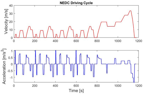
Figure 5.
The typical NEDC driving cycle used in the study: The driving cycle considers the 1180 s.
2.2. Parametric Study Using Design of Experiments (DoE)
A systematic parametric study was used to predict the effects of some important operating and design parameters on fuel economy. The parametric study executed using the multiphysics model was used as a data source for developing an Artificial Intelligence (AI) based machine learning model to be trained and used to predict efficiently the performance peaks of the fuel cell electric vehicle during driving. The procedure enables the effective coupled use of multiphysics simulation with statistical design of experiments and modern AI capabilities. For demonstration purposes, potential parameters were investigated using the introduced multiphysics model. The power peak in fuel economy was studied concerning its dependence on three factors, each set at three levels. In this context, the term factor is a variable, and the output is the numerical prediction of the average of power peaks within the initial driving phase as a parameter of interest. In order to investigate the parameters effectively being representative of an even larger data set presented in a compact form, an assembly of D-optimal analyses was implemented. It accounts for the interactions of the investigated parameters.
Classical fractional factorial designs were not used because they are not able to account for nonlinearities and interactions of the parameters, and the employment of full factorial plans would increase the required computational effort exponentially for demonstration purposes. D-optimal plans also require the least number of simulations and can accommodate both qualitative and quantitative variables, which might be of interest for future studies with more parameters. Details of the mathematical formulation of the D-optimality and D-criterion are given by Aguiar et al. [62] and were also used by the author of the current study in earlier optimisation studies [63]. For the assessment, computational simulations were performed based on an experimental design plan. The initial battery SOC, fuel cell maximum power, and vehicle weight were considered in the study as the variables. Their factor levels were set as −1, 0, and 1. They refer to the low, mid, and high levels of the factors, respectively. Other parameters were kept constant to assess the data quality to be processed in further AI-based model development. The investigated variables are given in Table 1.

Table 1.
Investigated parameters with feasible three levels referring to low, mid, and high levels of the variables.
The model configurations are simulated for 1180 s, mimicking the NEDC driving cycle. Despite the focus on generating and providing data for an AI-based machine learning model, for the sake of the reader, some details of the generated data are depicted in the next section.
2.3. Simulation Results
The results data given in Table 2 consider data that comprise all three levels of factors that were used in the study.
Table 2.
Used variable values for six different simulation configurations extracted from the complete DoE plan to predict the results of fuel economy and peaks during the NEDC.
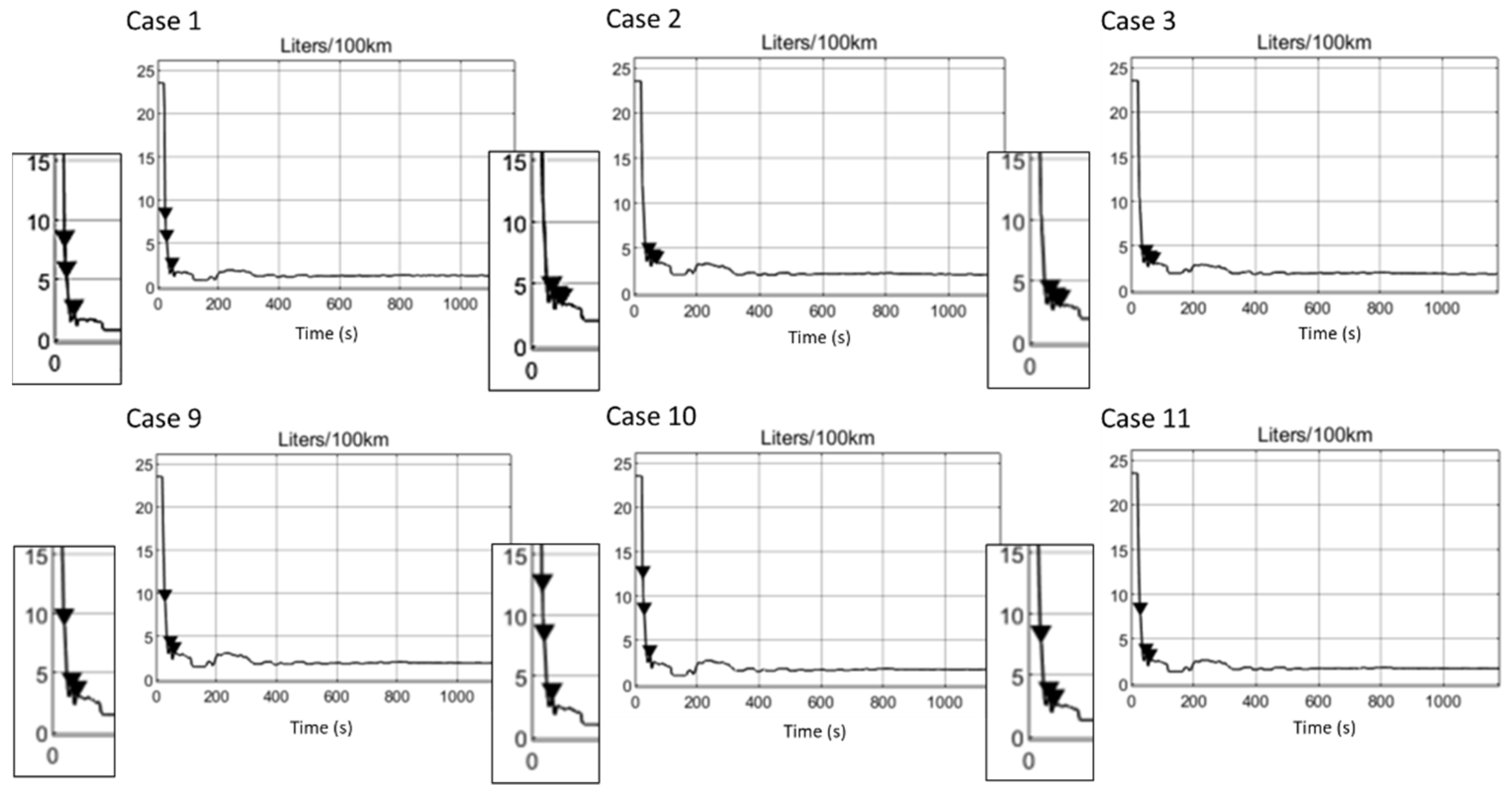
The simulated results shown in Figure 6 depict the fuel economy output predicted for the 1180 s NEDC duration and is based on the converted miles per gasoline-equivalent distribution over time. A total of 33.7 kilowatt-hours of electricity are equivalent to one U.S. gallon of gasoline or the equivalent of 235.125 L/100 km. The peak values are traced and depicted on each graph.
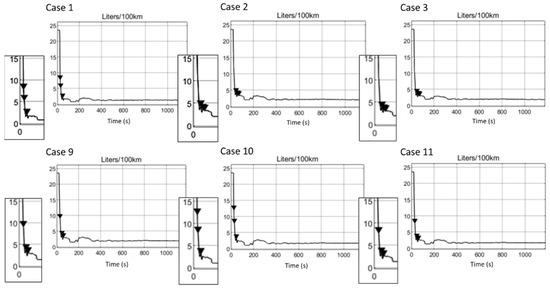
Figure 6.
Simulation results of fuel economy for the selected six different case files of the fuel cell electric vehicle.
The configurations for Case 2 and Case 3 show similar behaviour with the average of the three peaks showing values of 3.93; 3.27; 3.09 L/100 km and 4.41; 3.67; 3.47 L/100 km for Case 2 and Case 3, respectively. Comparing another pair, such as Case 1 and Case 3, shows that despite the vehicles having the same weight and slightly different maximum fuel cell power, the initial battery SOC difference of 0.2 resulted in remarkable maximum peak differences reaching close to 8 L/100 km in Case 1. The battery SOC data illustrated in Figure 7, together with the power supply, shed light on this behaviour, as the SOC characterises the remaining battery capacity as a percentage of the maximum capacity.

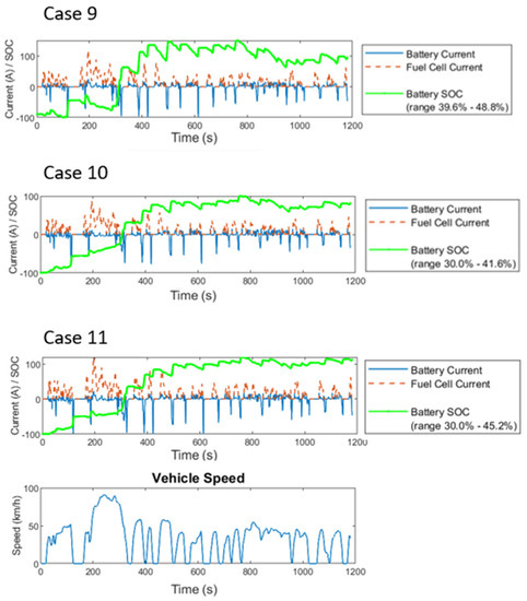
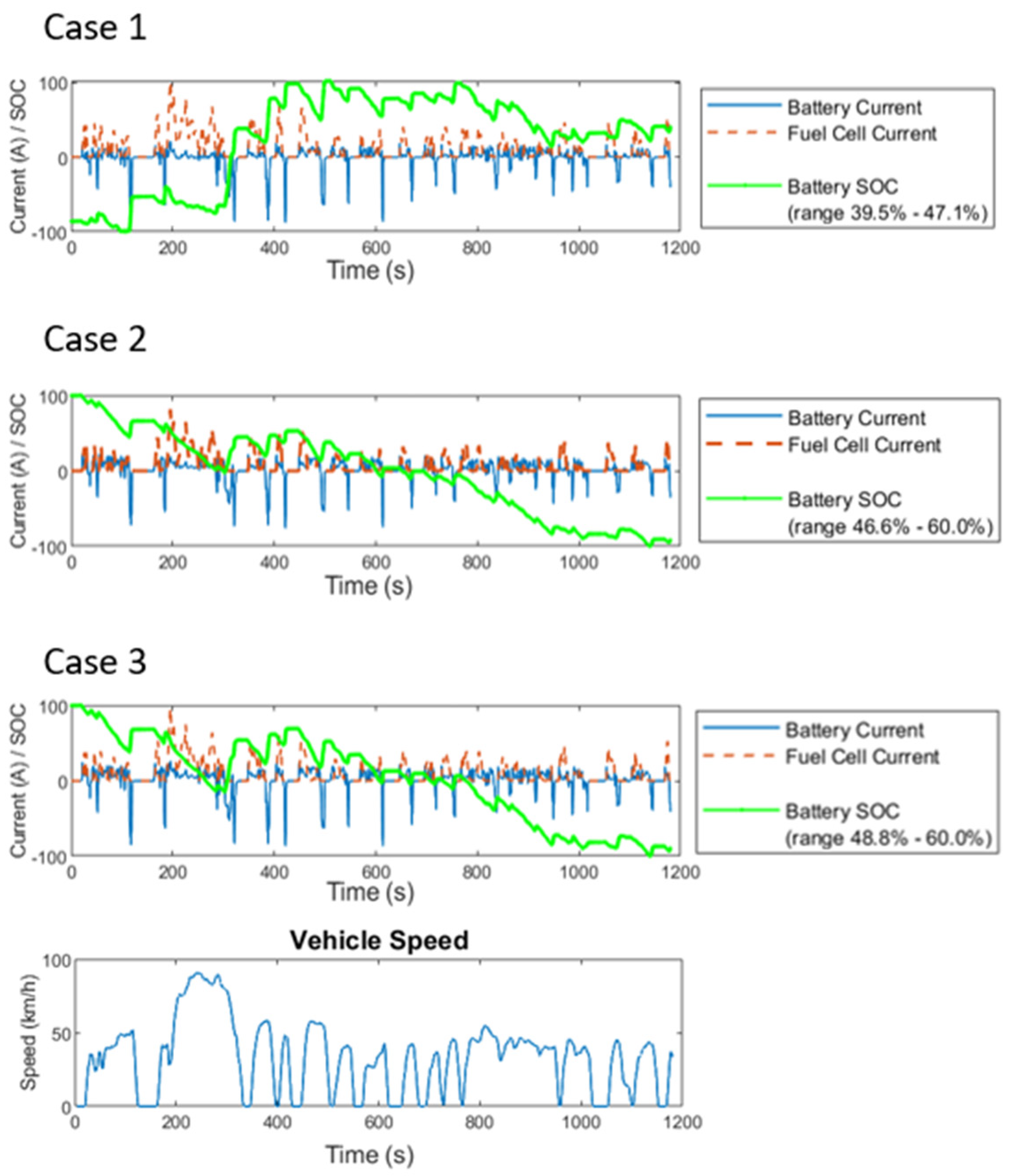
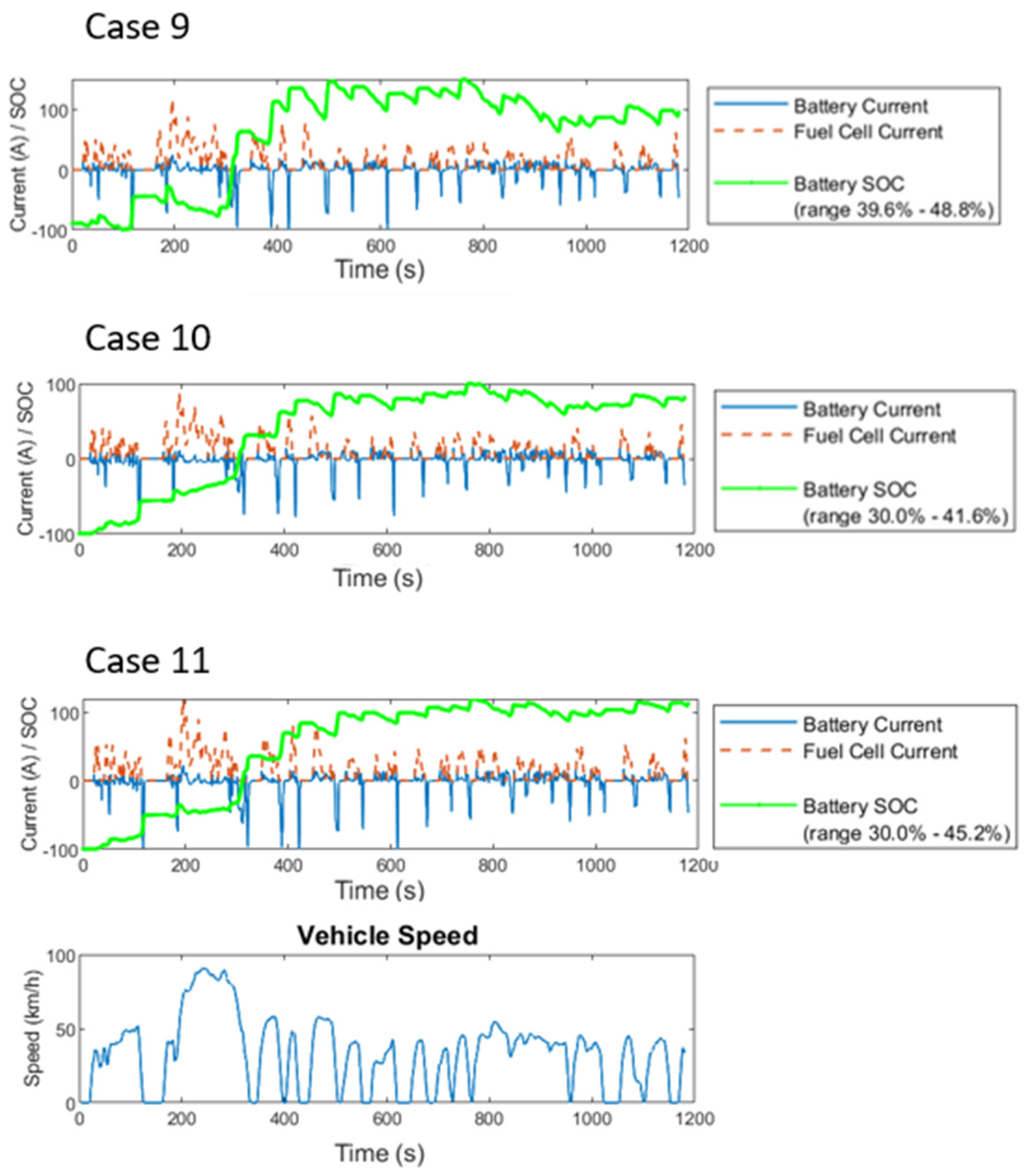
Figure 7.
Simulation results of the power supply for the selected six different case files of the fuel cell electric vehicle.
Case 1 shows the lower SOC value that starts to slowly increase from its initial 0.4 while the vehicle also speeds up. Case 2 and Case 3 that showed similar behaviour also reflect similar SOC distribution over time with slightly different ranges, but as expected, the decreasing behaviour explains the higher peaks in Case 1 compared to Case 2 and Case 3. Due to the changing veokhicle speed that is a function of the driving cycle, the operating conditions of the SOC are also affected in addition to changes in the voltage, charge/discharge current, and resistance parameters. Therefore, the drawn current varies, and the fuel cell provides more or less power accordingly. It is also interesting to observe the difference in the first peak between Case 1 and Case 9. The only parameter difference between those is their vehicle weight which is 300 kg. This difference appeared in the first peak for Case 1 with 7.87 L/100 km and 9.23 L/100 km for Case 9, respectively. Another final analysis may be the predicted highest peak in Case 10 due to the lower side of parameters resulting in much more power demand, thus higher values within this initial phase and reaching SOC values in the lower 40% range. For the sake of the focus of the study, more details and analysis of the data were not considered further.
3. Artificial Intelligence (AI) and Machine Learning (ML)
As technology has entered the age of artificial intelligence, the demand for digitally operating fast models transforming information has also reached an important stage. Increasingly sophisticated AI is expanding the impact of multiphysics modelling’s transformation. Traditional methods such as FEM/CFD were limited by the immense required user expertise as well as difficult to reach cost-effective solutions without setting systematic strategies. Since the new AI capabilities have collaborated with the vast number of high-end data provided by complex multiphysics analyses, an increasingly powerful breed of accelerated prediction and optimisation capability has been released. Large data sets can be stored and processed more conveniently, and the extracted digital representation of the actual problem becomes infinitely scalable. Thus, replicating the results can be shaped and enable various prediction options.
Through learning the introduced data and improving the algorithms that are embedded in AI-based technologies, a fundamental transformation in the modelling and simulation mindset was reached. There have been various applications of AI used in different industries, such as energy [64,65,66,67,68,69,70], transportation [71], medicine [72,73,74,75], and various other natural sciences [76,77,78]. Furthermore, the use and implementation of traditional modelling methods have been enhanced by collaborating with AI-based machine learning tools [79,80,81]. The current section briefly outlines the current AI-based machine learning methods that can be used in interdisciplinary fuel cell electric vehicle research to achieve an accelerated modelling workflow, improve understanding, optimise analyses, raise new questions, and seek new answers. This will adopt a successful human–computer interaction approach and establish a collective intelligence system based on the elements “What is being done?”, “By Whom?”, “Why?” and “How?” [82]. This section may be divided into subheadings. It should provide a concise and precise description of the experimental results, their interpretation, as well as the experimental conclusions that can be drawn.
3.1. Machine Learning (ML)
Artificial intelligence is an increasingly evolving field already supporting humans in making predictions about various interdisciplinary research areas. Artificial intelligence particularly aims to connect humans and computers in such a way that the combined level of intelligence increases. Widely accepted, one of the core AI methods used is machine learning (ML), which is a systematic approach that facilitates computers to learn from carefully collected and pre-processed data. The field of ML is tied to how humans learn; therefore, it attempts basically to understand and interpret data, algorithms, and theory comprising that. The goal is to bundle the methodologies embraced by basic human learning elements. Thereby using logic, deduction and backpropagation, programming, statistics, and probabilistic inference and making analogies to yield computational solutions.
The advantage of learning from a data set is that a human programmer is not required to set tasks. The connection between the programmer and the machine is such that they operate apart in comparison to traditional computer programming with direct commanding and receiving an answer. This is because the machine learning process is formulating decisions based on the supplied data, i.e., experience and replicating the process of human-based decision-making. These are derived by providing examples that show how the computer should proceed. The more complex the data pool, the more information can be gathered, but the more knowledge of the user is required. Thus, the learning process is driven by careful training. The process is highly dependent on the supplied and shaped data. Thus, it is a good platform for working with structured data sets, including tables of qualitative and quantitative variables. It seems to be overlapping with a similar term called data mining but differs in the way that machine learning has the central focus on self-learning from data and generating a model to provide the foundation for predictions for different scenarios, whereas data mining targets to recognise and detect patterns from large data sets to obtain insight from the past.
3.1.1. Supervised Learning
One of the cores of machine learning is the so-called supervised learning, which involves learning and understanding certain data through finding a relationship between variables and known results (response) and working with labelled data sets. The fact that both the variables and outputs are initially known entitles the data set as “labelled”. The mathematical algorithm then interprets the relationships and patterns that exist in the data and creates a mathematical model that can reproduce the same underlying rules with new data. Typical supervised learning comprises regression and classification problems. The cases where the response is a number are known as regression problems. Classification, on the other hand, in a simple context, involves multiple classes, and the input is assigned to one of the classes. Both regression and classification are concerned with the task of learning the mapping from the input variable to the response. The current study is a typical regression problem.
3.1.2. Unsupervised Learning
In the case of unsupervised learning, the supervisor is practically missing, and only the input data are present. Thus, not all variables and data patterns are known. Instead, the computer must detect hidden patterns and create labels using suitable learning algorithms. The difference is then to find the regularities in the input. This is analogue to density estimation, working with clusters in statistics. Data are grouped in data points that show similar features. The main benefit may be to be able to discover patterns within the data that have previously not been known, such as correlations or data clusters.
3.1.3. Reinforced Learning
The third and most advanced algorithm form in machine learning is reinforcement learning. The output of an investigated system is a sequence of actions, and a single response is not the focus. The sequence of right actions to reach a certain goal is the used approach. An action is right if it is part of a so-called policy. The learning process is based on appropriate past experiences to generate this kind of policy. Unlike supervised and unsupervised learning methods, the reinforcement learning approach continuously improves its model by gathering feedback from previous iterations in a loop. Thus, it does not approach an indefinite endpoint after the model is formulated from training and test data.
3.2. Deep Learning (DL)
Deep learning is the flagship of AI-based technology applications. It is principally a type of machine learning in which a model learns to perform classification tasks directly from acoustical signals, images, or various types of text. The method is usually applied using complex neural network architectures replicating the biological nervous system. The networks consist of various layers, and the number of these determines the depth of the created network, thus the term “deep”. Typical neural networks use lower numbers of layers, less than five, whereas deep networks reach beyond hundreds. The layers comprise an input layer, multiple hidden layers, and an output layer. All are connected through nodes, or the so-called neurons, where each hidden layer uses the output of the previous layer as its input data. These kinds of large networks are usually suitable for identification problems such as face recognition, various script and text translation, voice recognition, or advanced vehicle driver assistance systems. The connection to machine learning can be interpreted such that ML extracts features from data, whereas in deep learning, the data are directly fed into the generated neural network and let the features be learned automatically. For demonstration purposes, the current study also utilises a regression neural network model architecture fully connected and with feedforward features. This might be of interest and may show higher accuracy in case more complex data are used in future investigations.
3.3. Machine Learning Procedure
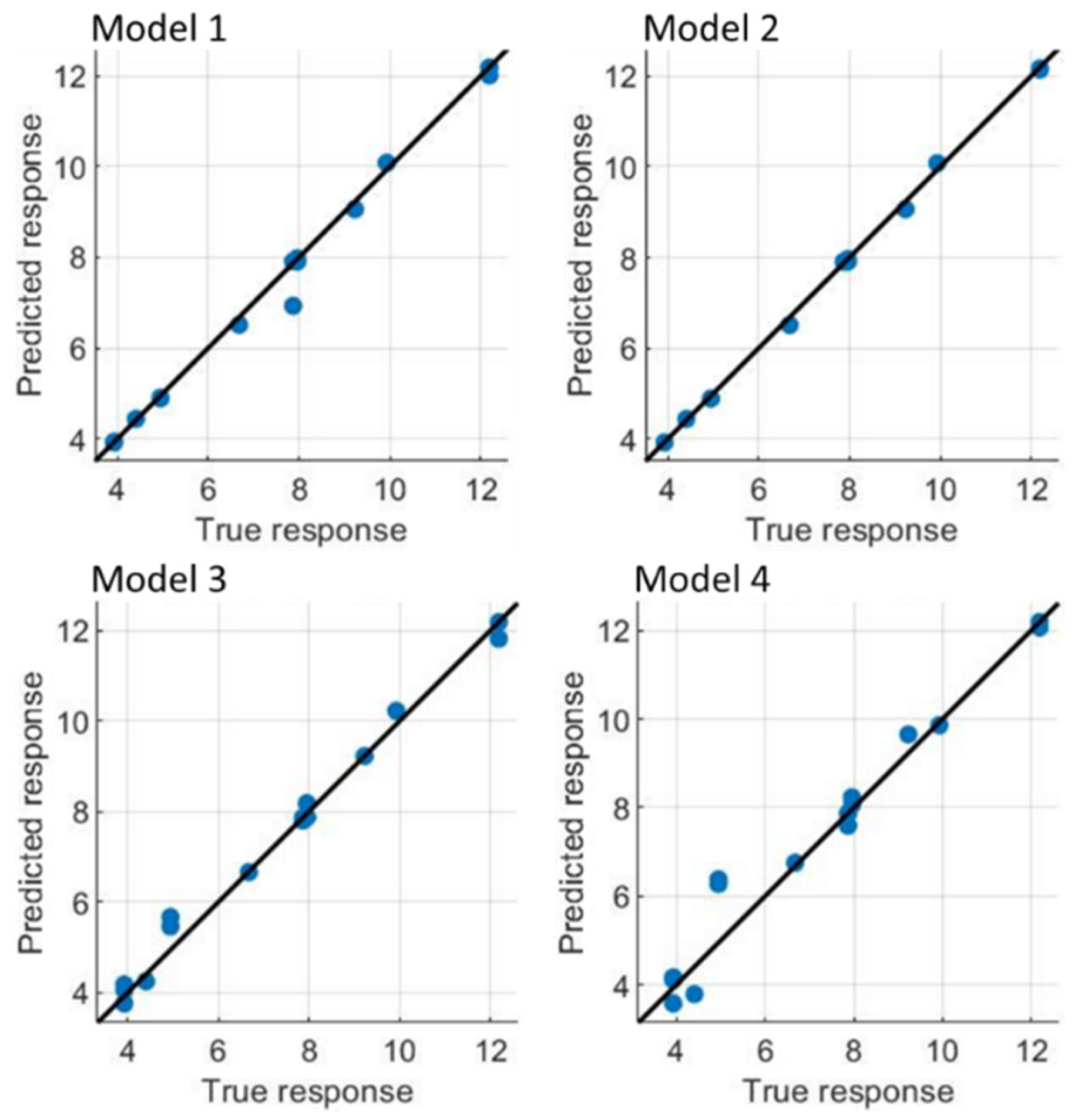
Based on the DoE-driven simulation results, a mathematical expression was derived considering the relation of the average of the three power peaks and the investigated parameters, i.e., the maximum fuel cell power, the initial SOC of the battery, and the vehicle’s weight. As the problem nature and data set fit well within the frame of a regression problem [83], statistical techniques were used to assess the relationship between the independent variables and the numeric response to predict the peaks in the fuel economy. The predicted response values vs. the true data points are plotted for four different regression models.
3.3.1. Model Development
The current study demonstrated the use of four different AI-based machine learning models. Model 1 is the well-known linear regression model that comprises the linear terms, an intercept, and all linear interactions of the variables, excluding squared terms. Model 2 considers a stepwise-linear variant. During regression, multiple variables are processed while simultaneously, the weakest correlated variable is removed. The variables that explain the distribution best are retained. Model 3 uses the correlation between the given different input data, where a covariance function learns the correlation among input data. For this purpose, a Gaussian process regression model [84] was tested. It is a model of probabilistic nature with the advantage of being nonparametric in comparison to more complex neural network models but, more importantly, also very convenient for training small-size data that are also valid for the present study. It interprets the response output by introducing latent variables from a set of random variables so that any finite number of them has a joint Gaussian distribution. Thus, it is the generalising of the well-known Gaussian distribution with the difference that is expressing the distribution among functions rather than being the distribution between random variables. Model 4 considers a feedforward neural network architecture with a fully connected layer of a single size. The first fully connected layer of the neural network has a connection with the input variables, and each subsequent layer has a connection with the previous layer. Each layer multiplies the input by a weight matrix and then adds a bias vector. A rectified linear unit (ReLU) activation function is transferring the sum of all weighted signals to a new activation value of that signal by monitoring each layer, excluding the last one, as the final fully connected layer produces then the neural network’s predicted response values.
3.3.2. Model Training
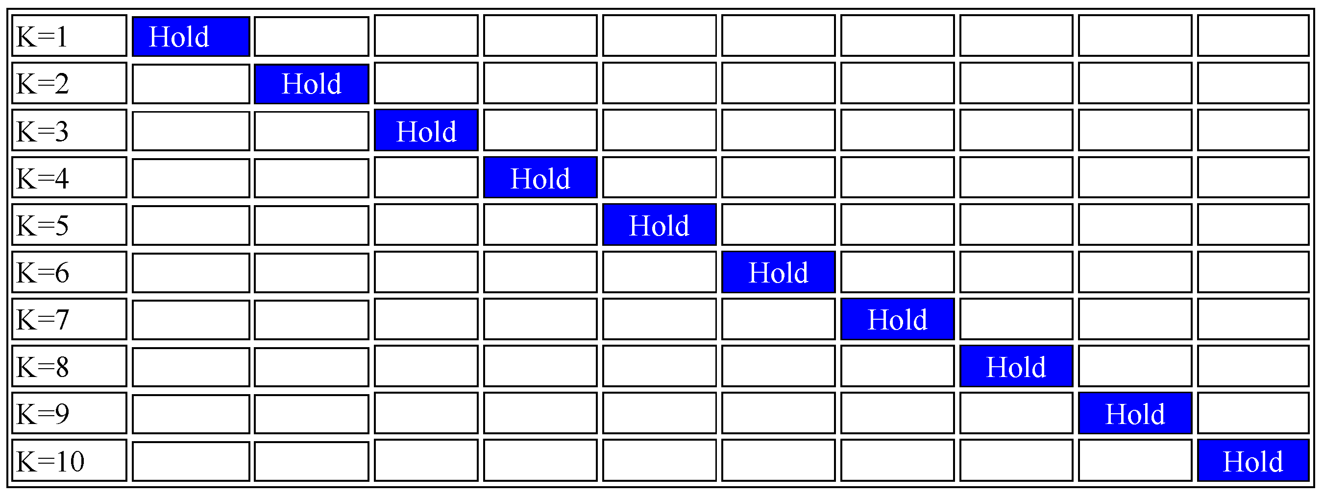
In machine learning, the proposed input data are partitioned into training data and test data. The same data are not used for both. If the developed model were used on the same data set, the model might be overfitted. The first split of the numerically calculated input data, i.e., the initial reserve of data that are used to develop the model, provides the training data. The training data are used to fit and tune the model, whereas the test set is put apart as “invisible” data to evaluate the accuracy of the model. If the model performs well on the training data but is poor on the separated test data, then it is considered to be overfitted. An important feature that needs to be considered while model training is that model parameters such as regression coefficients can be trained and learned directly from the proposed data set, but settings for the algorithms known as hyperparameters cannot be learned from these data. The training time limit or iteration number (defined in this study as 1000) needs to be set. In order to partition the user input data for training purposes, a cross-validation process is used. The data are split into sections, the so-called folds that train the model, and finally, calculate the average test error overall folds. The method is suitable for small data and mitigates overfitting. In this study, a ten-fold was chosen that can be explained, as illustrated in Figure 8.
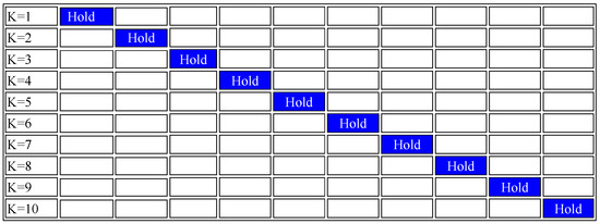
Figure 8.
Illustration of the cross-validation procedure used for partitioning input data into training and test data.
The training data are divided into 10 equal parts (folds), virtually creating 10 small train/test splits. The model was executed on nine folds (e.g., the last nine folds). The result was evaluated on the one remaining “hold” fold. Likewise, the iteration was performed ten times, each time holding a different fold. The results were averaged across all 10 hold folds and were interpreted to be the final performance estimate, i.e., the cross-validated score. The final tuning and fit of the model were then performed through the application of the cross-validation to each algorithm and, where appropriate, to the hyperparameters.
3.3.3. Model Results and Validation
In order to estimate the performance of the models, the accuracy needs to be assessed. The test set was used for this purpose. These were the second data that were generated during the partitioning process and have not been used yet during the training. All four models were evaluated, and the calculation of performance metrics was used to interpret the model accuracies. Once both the training data and test data were satisfactory, the machine learning model was ready to be used for further prediction of the peaks during the fuel economy. Figure 9 shows the results comparison of the models using the multiphysics simulations data.
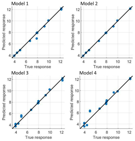
Figure 9.
Simulated data vs. machine learning model comparison using fuel economy peak as the response for the selected four different machine learning models.
The predicted response, i.e., the peak of fuel economy, is plotted along the vertical y-axis, and the true peak of the fuel economy is depicted along the horizontal x-axis. Points on the reference line indicate correct predictions. A good model produces predictions that are scattered close to the line, where the distance between the predicted values and the actual true values are called the residuals. The plotted results reveal promising results for all four configurations. Model 1 and Model 4 show slightly higher residuals compared to Model 2 and Model 3, which seem to show a better accuracy. Model 3 shows slightly higher deviations in the vicinity of the 4–6 values on the true response axis, suggesting that Model 2 is more accurate. In order to mitigate overfitting, i.e., the case in which the model is completely aligned to the training set but would not know how to respond to new data, the evaluation needs to be performed carefully. Therefore, the performance metrics for each model were calculated. The results are shown in Table 3.
Table 3.
Quality evaluation of the regression models considering R2, RMSE, MSE, and MAE for the trained model.
In order to interpret the goodness of the employed models, the mean squared error (MSE), root mean square error (RMSE), R-Squared (R2), and (MAE) were calculated and compared. The RMSE calculates the standard deviation of the error distribution of the data. The MSE value gives us the average squared difference between the predicted mean absolute error values and the actual true response values. The model with the lowest MSE is the model that is superior in predicting the actual values of the data set. The same applies to the MAE values, which is the arithmetic average of the absolute error gathered from the difference between the predicted and true values. Likewise, the R2 determines the reliability of the relationship between the models and the dependent variable on a 0–100% scale, where the higher values indicate a better fit. When comparing all model data, Model 2 reveals the best performance. The calculations show that unlike the initial interpretations from Figure 9, Model 1 shows, after Model 2, the lowest RMSE, MSE, and MAE values, suggesting that the error to the testing set in Model 3 and Model 4 is higher and the models became less accurate. It should be noted that the R2 values are also very close to each other, approaching 1, which indicates that the independent variables can explain most of the variability in the dependent variable. Hence, based on the overall results, Model 1 can be interpreted after Model 2 as the most accurate variant. This might also be due to the amount of data proposed. In the beginning, a model might seem very promising since the error to the training set might be lower. The best solution to this situation is to introduce more data. For the scope of the present study and the level of predicting capability satisfaction, Model 1 and Model 2 models will be used for prediction and evaluated with some multiphysics analyses for the used parameter values to observe the details and assess whether more data are needed. Another gain from the comparison is that it should be noted that each metric provides the analyst with different information. This can be better understood by comparing Model 1 and Model 3. The RMSE shows the typical distance between the predicted value made by the regression model and the actual value, whereas R2 indicates how well the predictor variables can explain the variation in the response variable. Despite the same R2 values, a difference in RMSE was determined.
3.4. Model Prediction Results
In order to perform predictions, Model 1 and Model 2 were further used. The parameters V1, V2, and V3 refer to the used parameters’ fuel cell power, initial battery SOC, and vehicle weight, respectively. The highest peak in fuel economy value predicted by the developed machine learning models was compared with the multiphysics model simulation results. The output is shown in Table 4.
Table 4.
Prediction of the highest fuel consumption peak value using machine learning models vs. the results predicted by the multiphysics simulation model.
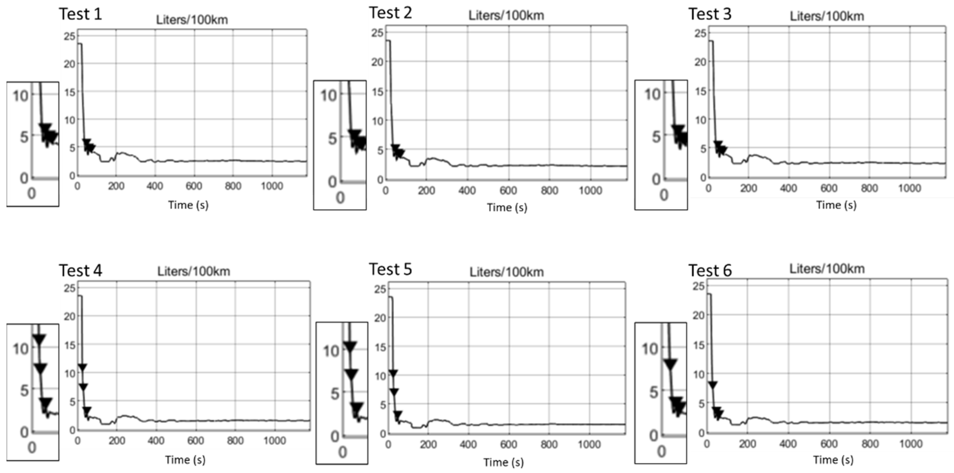
The results imply that an excellent agreement is achieved by predicting the highest peak value of the fuel economy using both machine learning models when compared with the results predicted by the multiphysics simulation model. Figure 10 depicts the detailed analysis of the demonstrated six predictions. Visible are the highest peaks among the three peaks in each graph. The highest fuel consumption is as expected with the lower side of SOCs despite the higher vehicle weight in the first three observations, as also shown in the detailed distribution for the given NEDC duration.
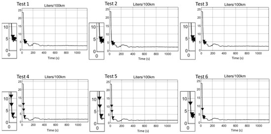
Figure 10.
Simulation results of fuel economy to verify the random data accuracy of the machine learning models using six new test files of the fuel cell electric vehicle model. The maximum values are in the close-up view illustrated.
It should be noted that the degree of random data set was appropriate because the new data set also considers values out of the subset used for training purposes. Thus, the accuracy was still valid, as verified with the new data set simulated and depicted in Figure 10. This reveals that the machine learning models provide an excellent first estimation and can be used as an optimisation tool that can highly accurately predict the peaks within the drive cycle under given parameters and reduce the overall consumption with particular targets such as under the desired 5 L/100 km range. It shows great potential to pre-select more parameters and predict different system or component behaviour within the complex vehicle.
4. Conclusions
This article aims to use emerging AI-based machine learning technologies to critically assess and discuss the fuel economy in fuel cell electric vehicles. Traditional multiphysics modelling results were obtained using a full fuel cell electric vehicle model, including powertrain and vehicle attributes, as well as an NEDC to predict real-life driving behaviour. A systematic D-optimal design plan was used to predict a representative pool of data that is used in developing and training a machine learning model. The comparison of training and test data results showed very good R2, RMSE, MSE, and MAE values for all the trained models. A step-wise linear and a linear regression type model revealed the best statistical evaluation results. Both models were used for further random prediction of fuel economy peaks within an NEDC. These data were also compared to detailed multiphysics analyses showing very good agreement. Their accuracy showed less than 1% error. The models proved to show very fast and good results. The study shows clearly that the combined use of AI-based machine learning with traditional multiphysics simulation and DoE is a very effective approach to be used for fuel cell electric vehicle assessment and optimisation purposes. Finally, the approach shows great potential in the accelerated data supply when more parameters are considered and trained using complex machine learning models.
Funding
This research received no external funding.
Data Availability Statement
Not applicable.
Conflicts of Interest
The author declares no conflict of interest.
References
- Le Den, X.; Bruyère, S.; Dubois, G.; Garcia-Borreguerro, C.; Bary, A. Feasibility and Scoping Study for the Commission to Become Climate Neutral by 2030 Final Report Commission to Become Climate Neutral by 2030. September 2020. Available online: https://op.europa.eu/en/publication-detail/-/publication/d3ecabf9-f895-11ea-991b-01aa75ed71a1 (accessed on 15 April 2022).
- Peksen, M. Hydrogen Technology towards the Solution of Environment-Friendly New Energy Vehicles. Energies 2021, 14, 4892. [Google Scholar] [CrossRef]
- Nanaki, E.A. Chapter 5—Climate change mitigation and electric vehicles. In Electric Vehicles for Smart Cities; Nanaki, E.A., Ed.; Elsevier: Amsterdam, The Netherlands, 2021; pp. 141–180. [Google Scholar] [CrossRef]
- Arora, S.; Abkenar, A.T.; Jayasinghe, S.G.; Tammi, K. Chapter 6—Charging Technologies and Standards Applicable to Heavy-duty Electric Vehicles. In Heavy-Duty Electric Vehicles; Arora, S., Abkenar, A.T., Jayasinghe, S.G., Tammi, K., Eds.; Butterworth-Heinemann: Oxford, UK, 2021; pp. 135–155. [Google Scholar] [CrossRef]
- Kittner, N.; Tsiropoulos, I.; Tarvydas, D.; Schmidt, O.; Staffell, I.; Kammen, D.M. Chapter 9—Electric vehicles. In Technological Learning in the Transition to a Low-Carbon Energy System; Junginger, M., Louwen, A., Eds.; Academic Press: Cambridge, MA, USA, 2020; pp. 145–163. [Google Scholar] [CrossRef]
- Andwari, A.M.; Pesiridis, A.; Rajoo, S.; Martinez-Botas, R.; Esfahanian, V. A review of Battery Electric Vehicle technology and readiness levels. Renew. Sustain. Energy Rev. 2017, 78, 414–430. [Google Scholar] [CrossRef]
- Çabukoglu, E.; Georges, G.; Küng, L.; Pareschi, G.; Boulouchos, K. Battery electric propulsion: An option for heavy-duty vehicles? Results from a Swiss case-study. Transp. Res. Part C Emerg. Technol. 2018, 88, 107–123. [Google Scholar] [CrossRef]
- Manzetti, S.; Mariasiu, F. Electric vehicle battery technologies: From present state to future systems. Renew. Sustain. Energy Rev. 2015, 51, 1004–1012. [Google Scholar] [CrossRef]
- Wang, C.; Zhou, S.; Hong, X.; Qiu, T.; Wang, S. A comprehensive comparison of fuel options for fuel cell vehicles in China. Fuel Process. Technol. 2005, 86, 831–845. [Google Scholar] [CrossRef]
- Kast, J.; Morrison, G.; Gangloff, J.J.; Vijayagopal, R.; Marcinkoski, J. Designing hydrogen fuel cell electric trucks in a diverse medium and heavy duty market. Res. Transp. Econ. 2018, 70, 139–147. [Google Scholar] [CrossRef]
- Lee, D.-Y.; Elgowainy, A.; Kotz, A.; Vijayagopal, R.; Marcinkoski, J. Life-cycle implications of hydrogen fuel cell electric vehicle technology for medium- and heavy-duty trucks. J. Power Source 2018, 393, 217–229. [Google Scholar] [CrossRef]
- Kast, J.; Vijayagopal, R.; Gangloff, J.J.; Marcinkoski, J. Clean commercial transportation: Medium and heavy duty fuel cell electric trucks. Int. J. Hydrogen Energy 2017, 42, 4508–4517. [Google Scholar] [CrossRef] [Green Version]
- Hernández-Torres, D.; Sename, O.; Riu, D.; Druart, F. On the Robust Control of DC-DC Converters: Application to a Hybrid Power Generation System. IFAC Proc. Vol. 2010, 43, 123–130. [Google Scholar] [CrossRef] [Green Version]
- Zhang, Z.; Wang, D.; Zhang, C.; Chen, J. Electric vehicle range extension strategies based on improved AC system in cold climate—A review. Int. J. Refrig. 2018, 88, 141–150. [Google Scholar] [CrossRef]
- Fernández, R.Á.; Cilleruelo, F.B.; Martínez, I.V. A new approach to battery powered electric vehicles: A hydrogen fuel-cell-based range extender system. Int. J. Hydrogen Energy 2016, 41, 4808–4819. [Google Scholar] [CrossRef]
- Millo, F.; Caputo, S.; Piu, A. Analysis of a HT-PEMFC range extender for a light duty full electric vehicle (LD-FEV). Int. J. Hydrogen Energy 2016, 41, 16489–16498. [Google Scholar] [CrossRef]
- Colloquium, A.; Technology, E.; Peksen, M. Fuel Cell Range Extender—Tailored System Development from Concept to Public Road Use. In Proceedings of the 8th Aachen Colloquium China, Beijing, China, 14–15 November 2018; pp. 1–7. [Google Scholar]
- Koj, J.C.; Wulf, C.; Zapp, P. Environmental impacts of power-to-X systems—A review of technological and methodological choices in Life Cycle Assessments. Renew. Sustain. Energy Rev. 2019, 112, 865–879. [Google Scholar] [CrossRef]
- Ahmadi, P.; Torabi, S.H.; Afsaneh, H.; Sadegheih, Y.; Ganjehsarabi, H.; Ashjaee, M. The effects of driving patterns and PEM fuel cell degradation on the lifecycle assessment of hydrogen fuel cell vehicles. Int. J. Hydrogen Energy 2019, 45, 3595–3608. [Google Scholar] [CrossRef]
- Weiss, M.; Irrgang, L.; Kiefer, A.T.; Roth, J.R.; Helmers, E. Mass- and power-related efficiency trade-offs and CO2 emissions of compact passenger cars. J. Clean. Prod. 2019, 243, 118326. [Google Scholar] [CrossRef]
- Götz, M.; Lefebvre, J.; Mörs, F.; McDaniel Koch, A.; Graf, F.; Bajohr, S.; Reimert, R.; Kolb, T. Renewable Power-to-Gas: A technological and economic review. Renew. Energy 2016, 85, 1371–1390. [Google Scholar] [CrossRef] [Green Version]
- Internacional Energy Agency. Renewable Energy Market Update; Internacional Energy Agency: Paris, France, 2021; p. 26. [Google Scholar]
- Jacob, J.; Pandey, A.; Rahim, N.A.; Selvaraj, J.; Samykano, M.; Saidur, R.; Tyagi, V. Concentrated Photovoltaic Thermal (CPVT) systems: Recent advancements in clean energy applications, thermal management and storage. J. Energy Storage 2021, 45, 103369. [Google Scholar] [CrossRef]
- Tarhan, C.; Çil, M.A. A study on hydrogen, the clean energy of the future: Hydrogen storage methods. J. Energy Storage 2021, 40, 102676. [Google Scholar] [CrossRef]
- Baykara, S.Z. Hydrogen: A brief overview on its sources, production and environmental impact. Int. J. Hydrogen Energy 2018, 43, 10605–10614. [Google Scholar] [CrossRef]
- Kumar, R.; Kumar, A.; Pal, A. An overview of conventional and non-conventional hydrogen production methods. Mater. Today Proc. 2021, 46, 5353–5359. [Google Scholar] [CrossRef]
- Abohamzeh, E.; Salehi, F.; Sheikholeslami, M.; Abbassi, R.; Khan, F. Review of hydrogen safety during storage, transmission, and applications processes. J. Loss Prev. Process Ind. 2021, 72, 104569. [Google Scholar] [CrossRef]
- Dawood, F.; Anda, M.; Shafiullah, G.M. Hydrogen Production for Energy: An Overview. Int. J. Hydrogen Energy 2020, 45, 3847–3869. [Google Scholar] [CrossRef]
- Peng, X.; Liu, Z.; Jiang, D. A review of multiphase energy conversion in wind power generation. Renew. Sustain. Energy Rev. 2021, 147, 111172. [Google Scholar] [CrossRef]
- Gandía, L.M.; Arzamendi, G.; Diéguez, P.M.; Varin, R.A.; Wronski, Z.S. Chapter 13—Progress in Hydrogen Storage in Complex Hydrides. Renew. Hydrog. Technol. 2013, 1, 293–332. [Google Scholar] [CrossRef]
- Ratnakar, R.R.; Gupta, N.; Zhang, K.; van Doorne, C.; Fesmire, J.; Dindoruk, B.; Balakotaiah, V. Hydrogen supply chain and challenges in large-scale LH2 storage and transportation. Int. J. Hydrogen Energy 2021, 46, 24149–24168. [Google Scholar] [CrossRef]
- Peksen, M. Chapter 1—Introduction to Multiphysics Modelling. In Multiphysics Modelling; Peksen, M., Ed.; Academic Press: Cambridge, MA, USA, 2018; pp. 1–35. [Google Scholar] [CrossRef]
- Korvink, J.G.; Greiner, A.; Liu, Z. 1.18—Multiphysics and Multiscale Simulation. Compr. Microsyst. 2008, 1, 539–557. [Google Scholar] [CrossRef]
- Lu, P.; Binita, B.; Barton, P.I.; Green, W.H. Reduced models for adaptive chemistry simulation of reacting flows. In Proceedings of the Second MIT Conference on Compurational Fluid and Solid Mechanics, Cambridge, MA, USA, 17–20 June 2003; pp. 1422–1425. [Google Scholar] [CrossRef]
- Lenczner, M.; Rochus, V. Special Issue: Multiphysics Modeling, Simulation and Experiments of Micro and Nanosystems. Mechatronics 2016, 40, 233–234. [Google Scholar] [CrossRef]
- Tian, F.; Voskuijl, M. Automated generation of multiphysics simulation models to support multidisciplinary design optimization. Adv. Eng. Inform. 2015, 29, 1110–1125. [Google Scholar] [CrossRef]
- Ramadesigan, V.; Northrop, P.W.C.; De, S.; Santhanagopalan, S.; Braatz, R.D.; Subramanian, V.R. Modeling and Simulation of Lithium-Ion Batteries from a Systems Engineering Perspective. J. Electrochem. Soc. 2012, 159, R31–R45. [Google Scholar] [CrossRef]
- Geng, C.; Jin, X.; Zhang, X. Simulation research on a novel control strategy for fuel cell extended-range vehicles. Int. J. Hydrogen Energy 2019, 44, 408–420. [Google Scholar] [CrossRef]
- Petersheim, M.D.; Brennan, S.N. Scaling of hybrid-electric vehicle powertrain components for Hardware-in-the-loop simulation. Mechatronics 2009, 19, 1078–1090. [Google Scholar] [CrossRef]
- Dai, H.; Zhang, X.; Wei, X.; Sun, Z.; Wang, J.; Hu, F. Cell-BMS validation with a hardware-in-the-loop simulation of lithium-ion battery cells for electric vehicles. Int. J. Electr. Power Energy Syst. 2013, 52, 174–184. [Google Scholar] [CrossRef]
- Tang, T.; Heinke, S.; Thüring, A.; Tegethoff, W.; Köhler, J. Freeze start drive cycle simulation of a fuel cell powertrain with a two-phase stack model and exergy analysis for thermal management improvement. Appl. Therm. Eng. 2018, 130, 637–659. [Google Scholar] [CrossRef]
- Zhang, C.; Santhanagopalan, S.; Sprague, M.; Pesaran, A.A. A representative-sandwich model for simultaneously coupled mechanical-electrical-thermal simulation of a lithium-ion cell under quasi-static indentation tests. J. Power Sources 2015, 298, 309–321. [Google Scholar] [CrossRef] [Green Version]
- Chen, J.; Huang, L.; Yan, C.; Liu, Z. A dynamic scalable segmented model of PEM fuel cell systems with two-phase water flow. Math. Comput. Simul. 2018, 167, 48–64. [Google Scholar] [CrossRef]
- Datta, D. Introduction to eXtended Finite Element (XFEM) Method. arXiv 2013, arXiv:1308.5208. [Google Scholar]
- Fotouhi, A.; Auger, D.J.; Propp, K.; Longo, S.; Wild, M. A review on electric vehicle battery modelling: From Lithium-ion toward Lithium–Sulphur. Renew. Sustain. Energy Rev. 2016, 56, 1008–1021. [Google Scholar] [CrossRef] [Green Version]
- Pelletier, S.; Jabali, O.; Laporte, G.; Veneroni, M. Battery degradation and behaviour for electric vehicles: Review and numerical analyses of several models. Transp. Res. Part B Methodol. 2017, 103, 158–187. [Google Scholar] [CrossRef]
- De Vita, A.; Maheshwari, A.; Destro, M.; Santarelli, M.; Carello, M. Transient thermal analysis of a lithium-ion battery pack comparing different cooling solutions for automotive applications. Appl. Energy 2017, 206, 101–112. [Google Scholar] [CrossRef]
- Xie, Y.; Li, J.; Yuan, C. Multiphysics modeling of lithium ion battery capacity fading process with solid-electrolyte interphase growth by elementary reaction kinetics. J. Power Source 2014, 248, 172–179. [Google Scholar] [CrossRef]
- Olivier, J.-C.; Wasselynck, G.; Chevalier, S.; Auvity, B.; Josset, C.; Trichet, D.; Squadrito, G.; Bernard, N. Multiphysics modeling and optimization of the driving strategy of a light duty fuel cell vehicle. Int. J. Hydrogen Energy 2017, 42, 26943–26955. [Google Scholar] [CrossRef]
- Hong, P.; Xu, L.; Li, J.; Ouyang, M. Modeling of membrane electrode assembly of PEM fuel cell to analyze voltage losses inside. Energy 2017, 139, 277–288. [Google Scholar] [CrossRef]
- Chavan, S.; Talange, D.B. Modeling and performance evaluation of PEM fuel cell by controlling its input parameters. Energy 2017, 138, 437–445. [Google Scholar] [CrossRef]
- Sezgin, B.; Caglayan, D.G.; Devrim, Y.; Steenberg, T.; Eroglu, I. Modeling and sensitivity analysis of high temperature PEM fuel cells by using Comsol Multiphysics. Int. J. Hydrogen Energy 2016, 41, 10001–10009. [Google Scholar] [CrossRef]
- Kakac, S.; Pramuanjaroenkij, A.; Zhou, X. A review of numerical modeling of solid oxide fuel cells. Int. J. Hydrogen Energy 2007, 32, 761–786. [Google Scholar] [CrossRef]
- Macedo-Valencia, J.; Sierra, J.; Figueroa-Ramírez, S.; Díaz, S.; Meza, M. 3D CFD modeling of a PEM fuel cell stack. Int. J. Hydrogen Energy 2016, 41, 23425–23433. [Google Scholar] [CrossRef]
- Kone, J.-P.; Zhang, X.; Yan, Y.; Hu, G.; Ahmadi, G. CFD modeling and simulation of PEM fuel cell using OpenFOAM. Energy Procedia 2018, 145, 64–69. [Google Scholar] [CrossRef]
- Peksen, M. Chapter 5—Multiphysics Modelling of Interactions in Systems. In Multiphysics Modelling; Peksen, M., Ed.; Academic Press: Cambridge, MA, USA, 2018; pp. 139–159. [Google Scholar] [CrossRef]
- Peksen, M. Safe heating-up of a full scale SOFC system using 3D multiphysics modelling optimisation. Int. J. Hydrogen Energy 2018, 43, 354–362. [Google Scholar] [CrossRef]
- Peksen, M. Numerical thermomechanical modelling of solid oxide fuel cells. Prog. Energy Combust. Sci. 2015, 48, 1–20. [Google Scholar] [CrossRef]
- Peksen, M. 3D transient multiphysics modelling of a complete high temperature fuel cell system using coupled CFD and FEM. Int. J. Hydrogen Energy 2014, 39, 5137–5147. [Google Scholar] [CrossRef]
- Al-Masri, A.; Peksen, M.; Khanafer, K. 3D multiphysics modeling aided APU development for vehicle applications: A thermo-structural investigation. Int. J. Hydrogen Energy 2019, 44, 12094–12107. [Google Scholar] [CrossRef]
- Tsiakmakis, S.; Fontaras, G.; Cubito, C.; Pavlovic, J.; Anagnostopoulos, K.; Ciuffo, B. From NEDC to WLTP: Effect on the Type-Approval CO2 Emissions of Light-Duty Vehicles; Publications Office of the European Union: Luxembourg, 2017. [Google Scholar] [CrossRef]
- de Aguiar, P.; Bourguignon, B.; Khots, M.; Massart, D.; Phan-Than-Luu, R. D-optimal designs. Chemom. Intell. Lab. Syst. 1995, 30, 199–210. [Google Scholar] [CrossRef]
- Peksen, M.; Blum, L.; Stolten, D. Optimisation of a solid oxide fuel cell reformer using surrogate modelling, design of experiments and computational fluid dynamics. Int. J. Hydrogen Energy 2012, 37, 12540–12547. [Google Scholar] [CrossRef]
- Javadi, A.; Faramarzi, A.; Ahangar-Asr, A. An Artificial Intelligence Based Finite Element Method Offshore Wind Tur-Bines View Project Optimisation of Enhanced Geothermal Systems View Project. 2009. Available online: https://www.researchgate.net/publication/260125327 (accessed on 15 April 2022).
- Miraftabzadeh, S.; Longo, M.; Foiadelli, F.; Pasetti, M.; Igual, R. Advances in the Application of Machine Learning Techniques for Power System Analytics: A Survey. Energies 2021, 14, 4776. [Google Scholar] [CrossRef]
- He, Q.; Zheng, H.; Ma, X.; Wang, L.; Kong, H.; Zhu, Z. Artificial intelligence application in a renewable energy-driven desalination system: A critical review. Energy AI 2021, 7, 100123. [Google Scholar] [CrossRef]
- Nti, E.K.; Cobbina, S.J.; Attafuah, E.E.; Opoku, E.; Gyan, M.A. Environmental Sustainability Technologies in Biodiversity, Energy, Transportation and Water Management using Artificial Intelligence: A Systematic Review. Sustain. Futures 2022, 4, 100068. [Google Scholar] [CrossRef]
- Wei, H.; Bao, H.; Ruan, X. Perspective: Predicting and optimizing thermal transport properties with machine learning methods. Energy AI 2022, 8, 100153. [Google Scholar] [CrossRef]
- Zhao, X.; Li, B. The countermeasures of urban energy risk control oriented to machine learning and data fusion. Energy Rep. 2022, 8, 2547–2557. [Google Scholar] [CrossRef]
- Gan, M.; Hou, H.; Wu, X.; Liu, B.; Yang, Y.; Xie, C. Machine learning algorithm selection for real-time energy management of hybrid energy ship. Energy Rep. 2022, 8, 1096–1102. [Google Scholar] [CrossRef]
- Bachute, M.R.; Subhedar, J.M. Autonomous Driving Architectures: Insights of Machine Learning and Deep Learning Algorithms. Mach. Learn. Appl. 2021, 6, 100164. [Google Scholar] [CrossRef]
- Chew, A.W.Z.; Zhang, L. Data-driven multiscale modelling and analysis of COVID-19 spatiotemporal evolution using explainable AI. Sustain. Cities Soc. 2022, 80, 103772. [Google Scholar] [CrossRef] [PubMed]
- Wang, Z. Use of supervised machine learning to detect abuse of COVID-19 related domain names. Comput. Electr. Eng. 2022, 100, 107864. [Google Scholar] [CrossRef] [PubMed]
- Macpherson, T.; Churchland, A.; Sejnowski, T.; DiCarlo, J.; Kamitani, Y.; Takahashi, H.; Hikida, T. Natural and Artificial Intelligence: A brief introduction to the interplay between AI and neuroscience research. Neural Netw. 2021, 144, 603–613. [Google Scholar] [CrossRef] [PubMed]
- Hassan, H.; Ren, Z.; Zhou, C.; Khan, M.A.; Pan, Y.; Zhao, J.; Huang, B. Supervised and weakly supervised deep learning models for COVID-19 CT diagnosis: A systematic review. Comput. Methods Programs Biomed. 2022, 218, 106731. [Google Scholar] [CrossRef]
- Syed, F.I.; AlShamsi, A.; Dahaghi, A.K.; Neghabhan, S. Application of ML & AI to model petrophysical and geomechanical properties of shale reservoirs—A systematic literature review. Petroleum 2022, 8, 158–166. [Google Scholar] [CrossRef]
- Elbasheer, M.; Longo, F.; Nicoletti, L.; Padovano, A.; Solina, V.; Vetrano, M. Applications of ML/AI for Decision-Intensive Tasks in Production Planning and Control. Procedia Comput. Sci. 2022, 200, 1903–1912. [Google Scholar] [CrossRef]
- Vadyala, S.R.; Betgeri, S.N.; Matthews, J.C.; Matthews, E. A review of physics-based machine learning in civil engineering. Results Eng. 2021, 13, 100316. [Google Scholar] [CrossRef]
- Usman, A.; Rafiq, M.; Saeed, M.; Nauman, A.; Almqvist, A.; Liwicki, M. Machine Learning Computational Fluid Dynamics. In Proceedings of the 2021 Swedish Artificial Intelligence Society Workshop (SAIS), Luleå, Sweden, 14–15 June 2021; pp. 1–4. [Google Scholar] [CrossRef]
- Lv, M.; Zhao, J.; Cao, S.; Shen, T. Prediction of the 3D Distribution of NOx in a Furnace via CFD Data Based on ELM. Front. Energy Res. 2022, 10, 93. [Google Scholar] [CrossRef]
- Calzolari, G.; Liu, W. Deep learning to replace, improve, or aid CFD analysis in built environment applications: A review. Build. Environ. 2021, 206, 108315. [Google Scholar] [CrossRef]
- Malone, T.W.; Bernstein, M.S. Handbook of Collective Intelligence; MIT Press: Cambridge, MA, USA, 2015. [Google Scholar]
- Fernández-Delgado, M.; Sirsat, M.; Cernadas, E.; Alawadi, S.; Barro, S.; Febrero-Bande, M. An extensive experimental survey of regression methods. Neural Netw. 2018, 111, 11–34. [Google Scholar] [CrossRef]
- Li, P.; Chen, S. A review on Gaussian Process Latent Variable Models. CAAI Trans. Intell. Technol. 2016, 1, 366–376. [Google Scholar] [CrossRef]


Publisher’s Note: MDPI stays neutral with regard to jurisdictional claims in published maps and institutional affiliations. |
© 2022 by the author. Licensee MDPI, Basel, Switzerland. This article is an open access article distributed under the terms and conditions of the Creative Commons Attribution (CC BY) license (https://creativecommons.org/licenses/by/4.0/).