1. Introduction
The mining industry has been under increasing pressure to innovate as mining companies look for different ways to decrease cost in the face of a downward trend in profits. This has led the industry to adopt autonomous driving solutions for mining operations due to the repetitiveness of several mining tasks. Autonomous driving technology can lead to the improvement of the overall safety of the mine, an increase in productivity and efficiency, and a decrease in operating costs [
1]. The use of autonomous machinery has also been promoted in countries with declining birth rates and aging populations as a solution to maintain productivity in these areas [
2].
Load-haul-dump (LHD) operations are one of many types of operations that are common to trucks-including mining trucks. They usually involve loading of materials to be hauled and then unloading, or dumping, at the destination point. This process is then repeated from the destination point to the next point. Truck autonomy plays a promising role in increasing the safety and efficiency of these operations due to the repetitiveness of such an operation [
3].
Automation of underground mining LHD vehicles has gathered increased interest due to the hazardous nature of such an environment. In [
4], the authors propose using laser scanners and reference strips to guide an underground LHD vehicle through the operation. Wall-following in [
5] was proposed as an alternative technique for underground navigation that did not require special infrastructure. Building on this technique, the work in [
6] proposed a reactive wall-following navigation system complemented with weak localization that achieved near-human performance at full-speed on a LHD operation in a real underground test mine. Other works have focused on the modeling and control of mining vehicles using mathematical modeling and simulation [
7,
8,
9,
10,
11] and small-scale environments [
12].
However, in order to facilitate the testing of autonomous solutions, a simulation environment is necessary to decrease the cost of development and deployment-especially as these machinery can be costly. Such a simulation environment needs to be able to accurately model vehicle dynamics, to capture interactions with obstacles, and to provide sensing capabilities such as LiDAR, camera, and GPS. The latter provides freedom in testing different sensing configurations. Such a requirement extends beyond conventional methods of mathematical simulation and lab-scale environments.
In this paper, we will use the example of a surface mine and an articulated dump truck to provide a framework for the automation of a generic load-haul-dump process. Unlike previous works, we will propose a realistic model of our vehicle using rigid-body dynamics in a 3D physics-based simulation environment to study the performance of the proposed approach. Such a simulation setup would allow for more accurate interaction with the physical system. While the operation and simulation environment can be adapted to different environments, we will focus solely on a surface mine as a generic example in the work presented.
2. Methods
2.1. Scenario Description
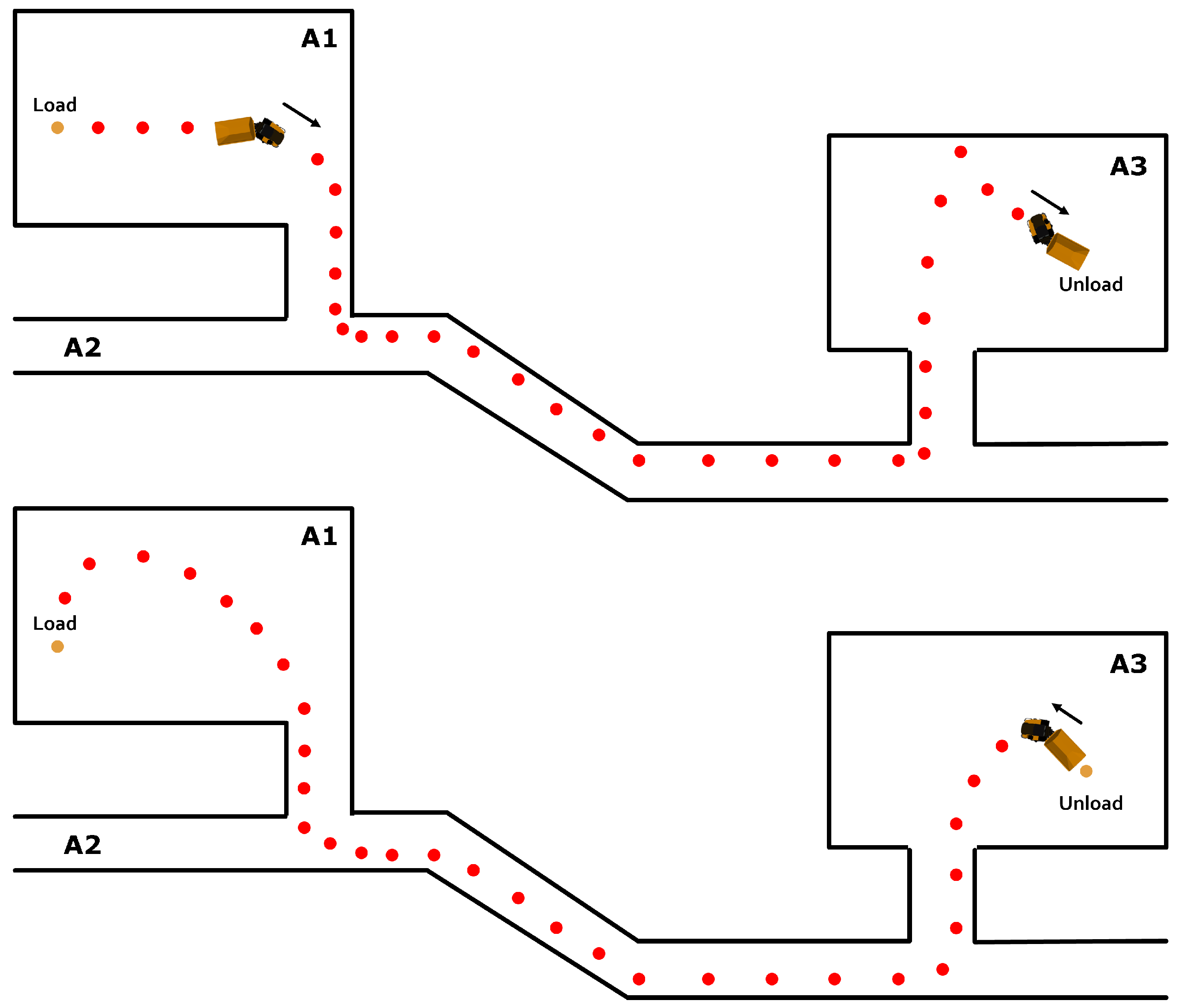
We consider the load-haul-dump operation of a six-wheeled articulated dump truck (ADT) in a surface mine environment as shown in
Figure 1. The environment consists of three areas: A1 as the loading area, A3 as the unloading area, and A2 as the roadway connecting A1 and A3. In this analysis, we assume that there exists one ADT and no other traffic present. The goal of the ADT is to perform a series of operations to move autonomously between the load and unload areas along A2.
To do so, a road topology needs to be defined so that the truck can perform the appropriate decisions based on its current situation. The road topology refers to the different layouts in the network of the road. For example, an intersection or a two-way road. These are mapped as waypoints that are used to indicate to the vehicle its current state along the operation. In general, we have followed the terminology and conventions used in the DARPA Urban Challenge for the road specification [
13]. This road definition and the operation can be then defined as follows,
Separate waypoints are defined for the load, haul, and unload areas in each direction.
Waypoint files start and end at a checkpoint.
T-junctions are given in terms of checkpoints, waypoints, and intersection geometry.
The speed is adjusted along roadway to speed up, cruise, and decelerate so as to stop at a checkpoint at the end of the roadway or a T-junction in either direction.
It is important to note that the roadway is not defined in terms of the road edges as it is assumed that it cannot be sensed. It is also assumed that the waypoint files are established by driving along each lane and listing the measured GPS positions at regular intervals. This allows for virtual lane edges to be drawn on the map based on the assumed width of each lane or roadway. In this work, traffic is assumed to drive on the left side.
2.2. Scenario Analysis and Design
The scenario described presents a fixed operation. That is: the goals are the same, the operations are repeated, and the sequence of operations is known a-priori.
2.2.1. End-to-End Operational Decomposition
An end-to-end operational decomposition allows the system to be represented as a Discrete Event System (DES). A Finite State Machine (FSM) can then be created to represent the DES and form the high-level decision-making module of the autonomous vehicle [
14,
15]. The 13-stage decomposition for the full operational cycle (load-haul-unload-haul-load) is given as follows:
A1: Load.
A1: Move to intersection, evading obstacles.
T-junction: Turn onto road (left turn).
A2: Travel along road.
T-junction: Turn off road at entrance of A3 (left turn).
A3: Move to unloading position.
A3: Unload.
A3: Move to intersection.
T-junction: Turn onto road (right turn).
A2: Travel along road.
T-junction: Turn off road at A1 (right turn).
A1: Move to loading position, evading obstacles.
A1: Stop/Wait.
2.2.2. Finite State Machine
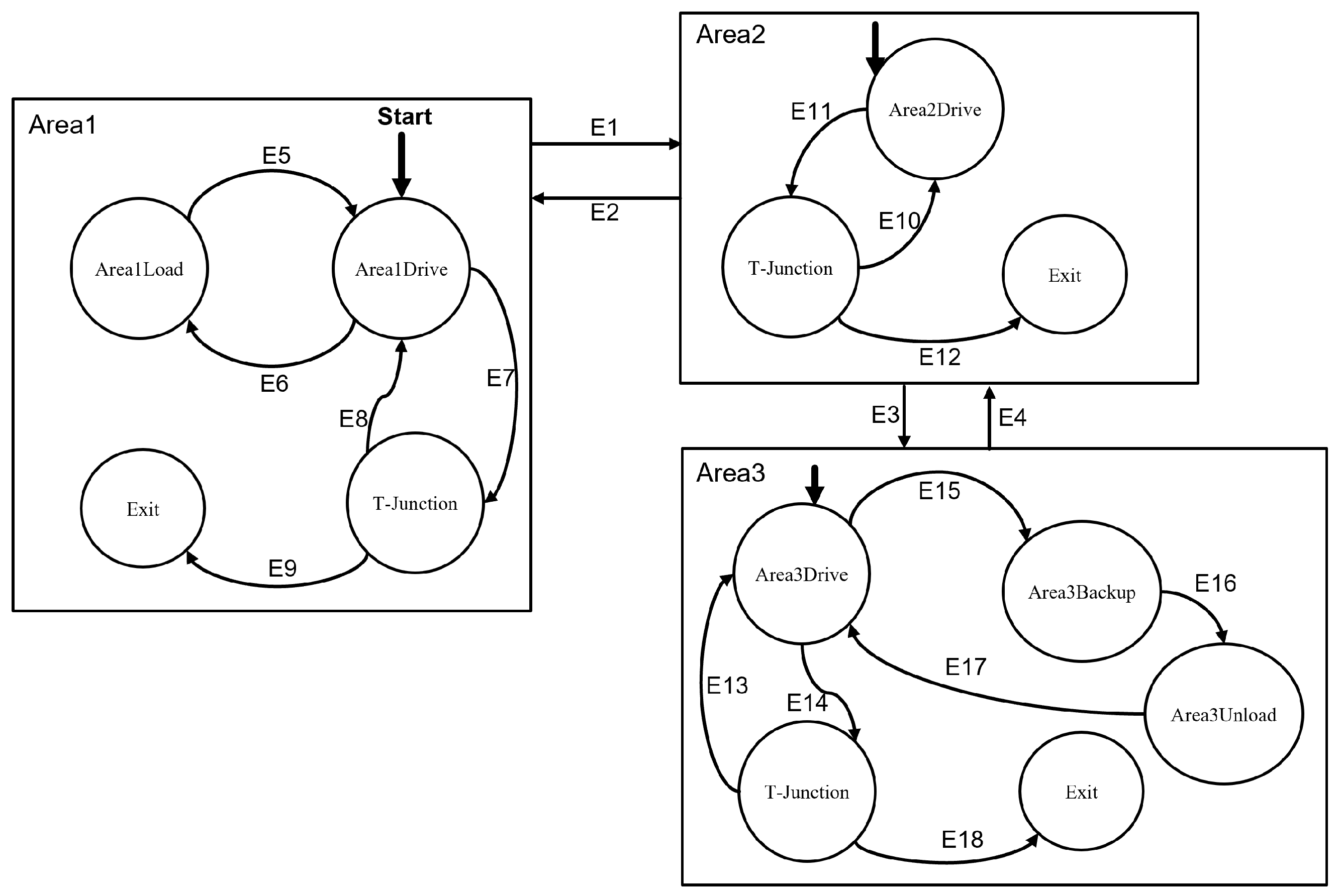
Each stage of the operation represents a meta-state in the FSM and the checkpoints in the road topology defined determine the state transitions. The operational meta-states listed can be further grouped into three larger meta-states each pertaining to A1, A2, and A3 operation as outlined in
Figure 2. Hence, each area has a group of operational meta-states that defines the truck’s maneuver and these areas are transitioned through the T-junction states. The loading state of the truck determines whether the truck is moving towards A1 (unload-haul-load operation) or A3 (load-haul-unload operation). Waypoints and the GPS position indicate to the vehicle what meta-state in the FSM to use. The state transition events are defined in
Table 1.
2.3. Simulation Environment
To facilitate the testing of autonomous vehicle algorithms, we develop a 3D physics-based simulation environment coined as the Oztech Modular Design Environment (
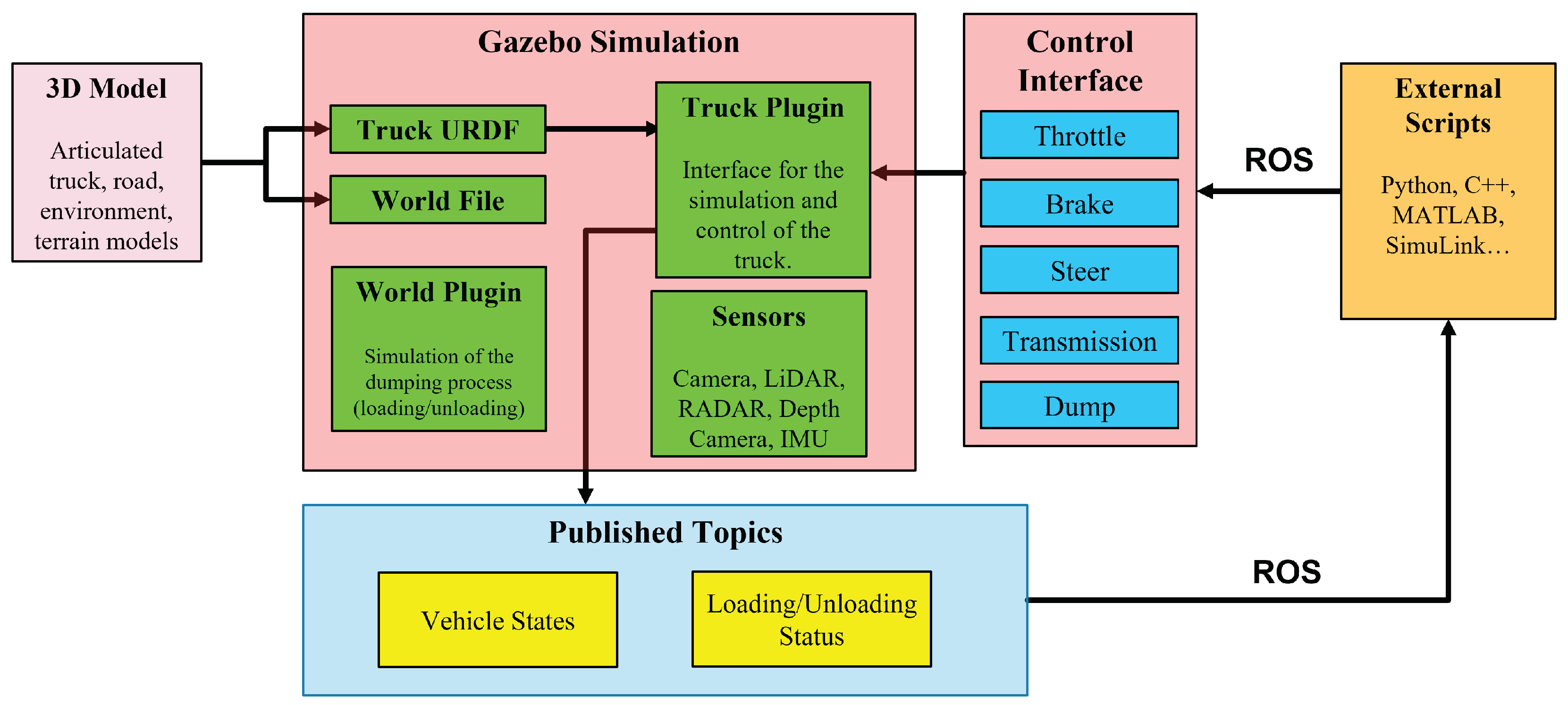
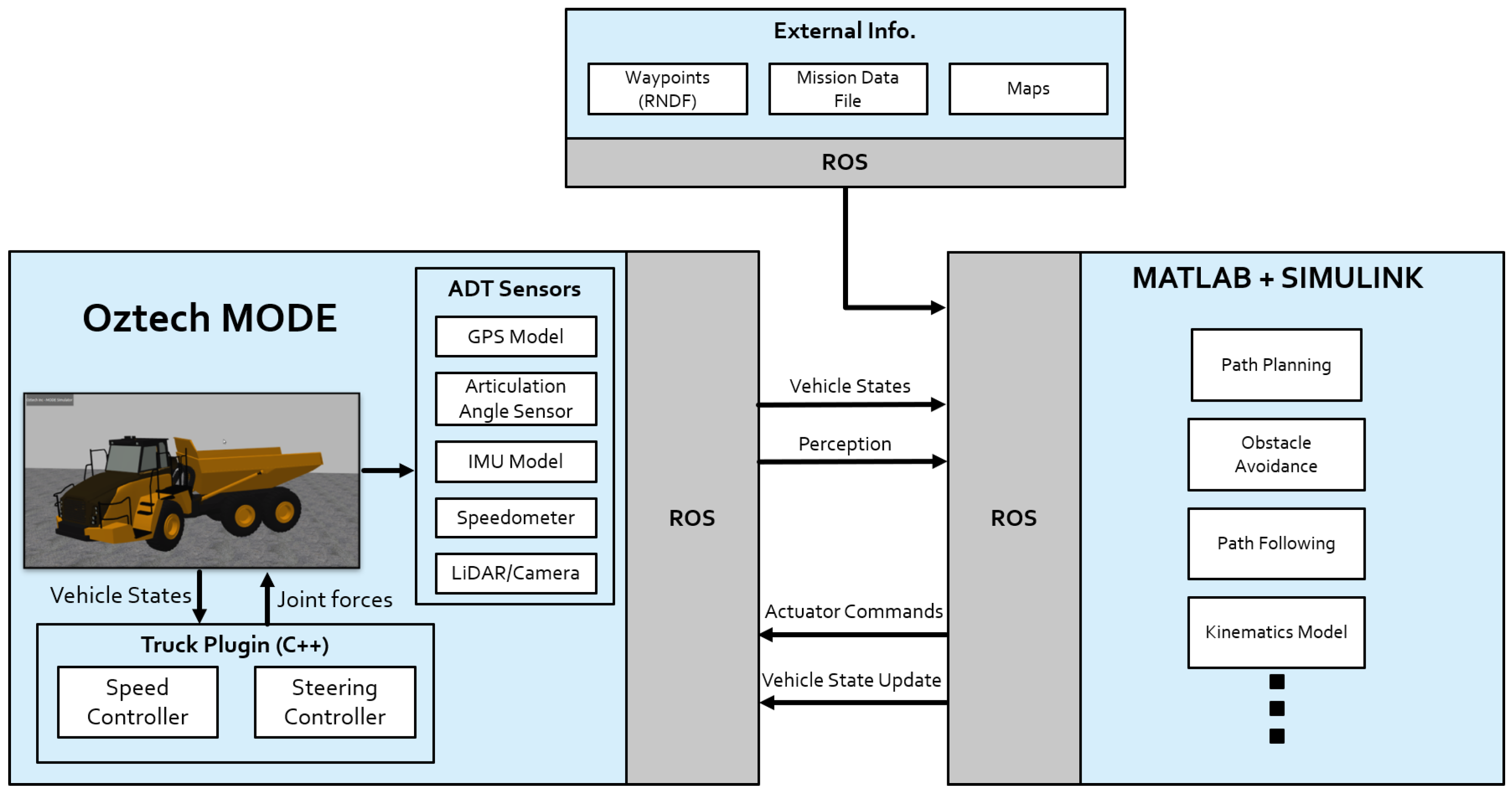
MODE), to represent a realistic model of the vehicle and its dynamics, the physical environment, and the sensor suite. This simulation environment was built on top of the Gazebo simulator, which is a popular 3D robotics simulator, and the ROS framework. The environment also provides an appropriate control interface with the simulated vehicle and external scripts so as to alter the simulation. The architecture of the simulation environment is shown in
Figure 3. We leverage the existing Gazebo physics engine, 3D visualization capabilities, and base sensor suite while building the rest of the modules shown in the architecture.
2.3.1. Environment Model
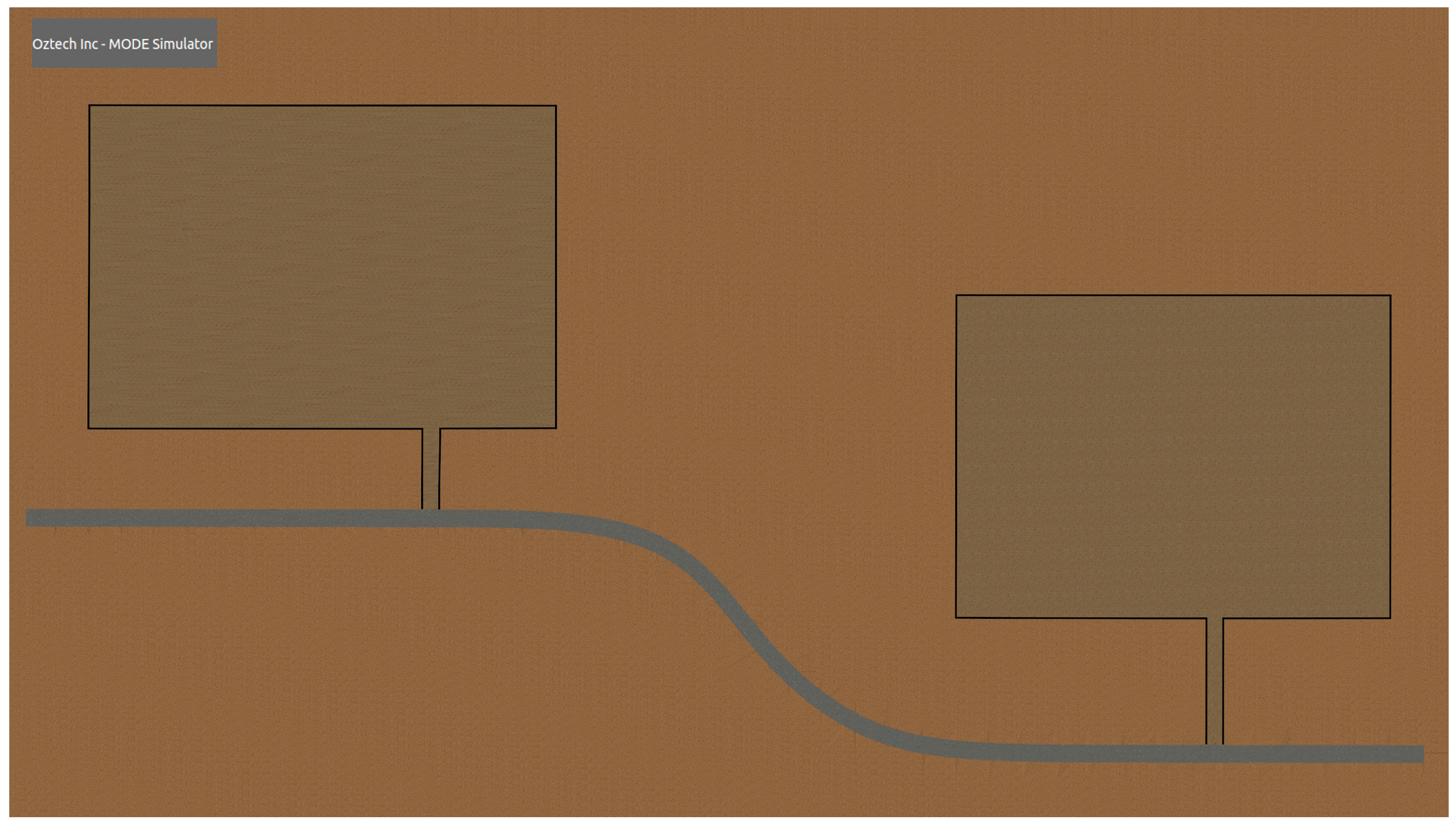
An environment model shown in
Figure 4 was developed in Blender to represent the given operation description (
Figure 1). The environment consists of two areas, loading and unloading, and an asphalt road connecting the two areas. A T-junction exists at the entrance/exit of each area to the roadway.
2.3.2. Truck Model
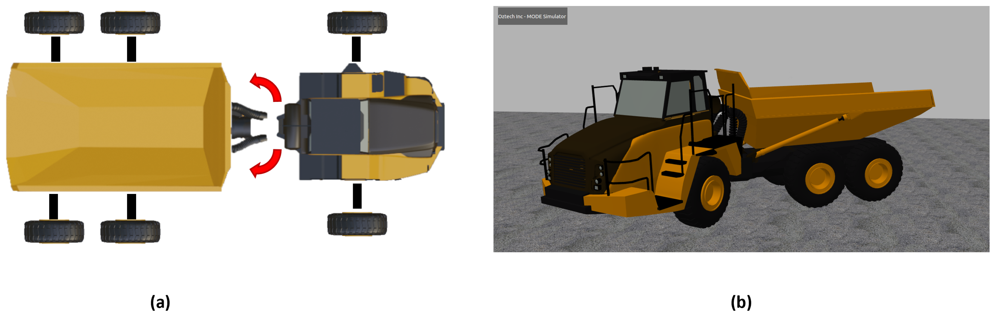
A realistic model of the ADT was constructed based on the physical, inertial, and geometrical properties of a commercial articulated truck [
16]. The ADT was modeled using rigid-body dynamics and constructed as a multibody system: two rigid bodies connected through a hinge joint at the articulation point. The truck model and the construction of the different body links and joint connections are shown in
Figure 5. A plugin was also developed to simulate the actuation dynamics of the truck. Namely, the suspension, the steering, the throttle, and the brake actuation. The steering is controlled using a PID controller to produce the required torque at the hinge joint based on the steering error. The throttle and brake actuation is modeled using simple linear models as a function of the pedal or brake percentage and total torque. These result in approximations of the engine dynamics of the vehicle as the full powertrain and tire dynamics are not considered. The suspension is modeled as a spring-mass-damper system. The plugin also provides the control interface with the actuators over ROS.
2.3.3. Sensing
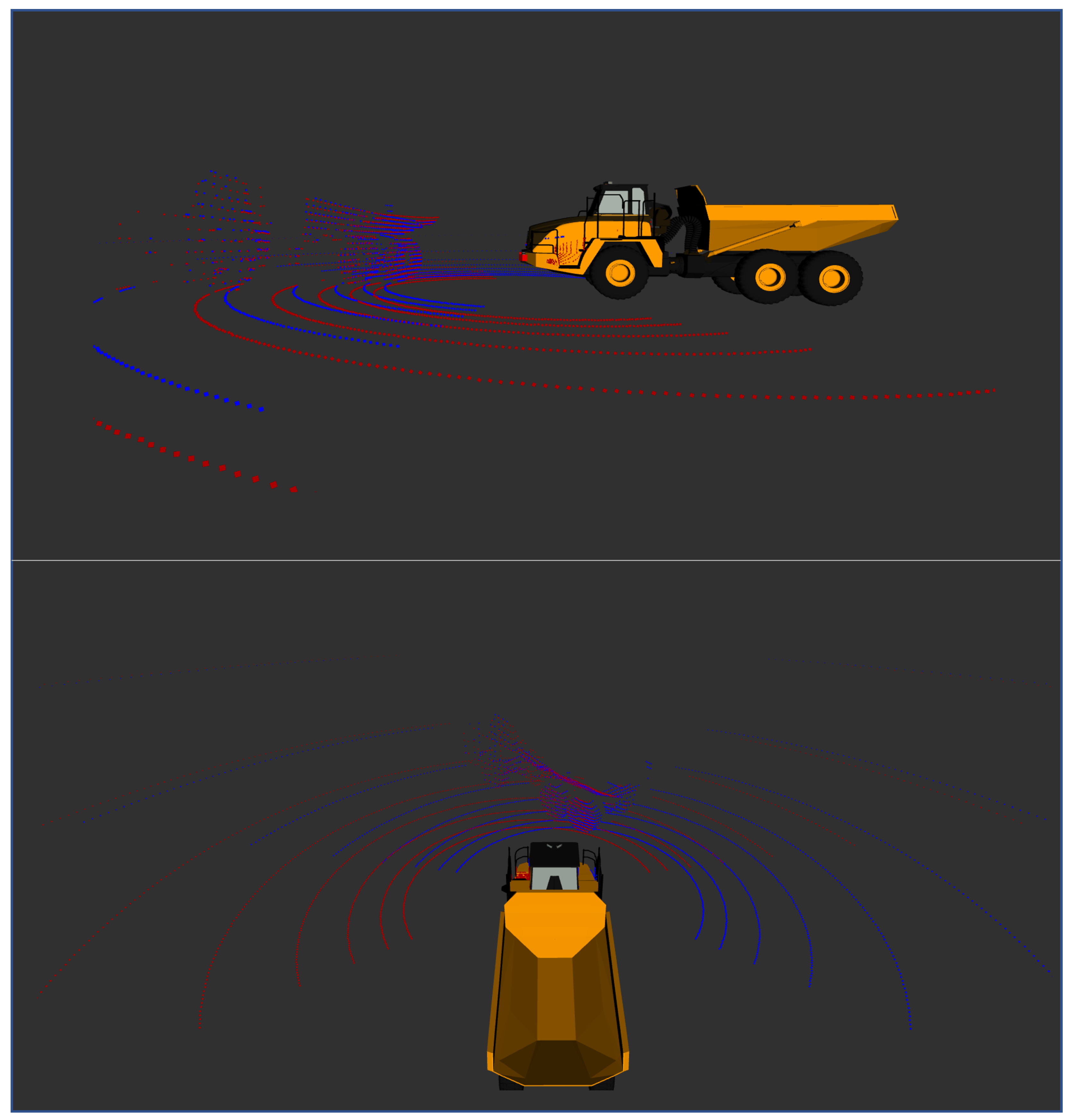
Simulation provides the capability of testing different sensor configurations at no additional cost. Therefore, a strong sensor suite is important in the development of a simulator for autonomous vehicle testing. The developed simulation environment leverages the sensor suite found in the Gazebo simulator: stereo cameras, depth cameras, LiDAR, and RADAR; and extends the sensing capabilities to include an articulation angle sensor for steering control, and a GPS module for localization. The sensors output their data over the ROS framework as ROS topics that allow external scripts to access the data. The sensor output can also be visualized in rviz in real-time. An example of the sensor view is shown in
Figure 6.
2.3.4. MATLAB Integration
The simulation environment provides an integration interface with MATLAB and Simulink through the ROS framework as shown in
Figure 7. This allows for the operation control architecture to be developed externally but simulated on our vehicle model and environment.
2.4. Path Tracking
The path tracking criterion and state vector construction is based on the work of [
17]. It is assumed that a path is already planned and that the operation of the ADT follows the given operational decomposition. Hence the high-level control is decided by the Finite State Machine defined and the path tracking controller implements the low-level control. This subsection focuses solely on the path tracking problem.
2.4.1. Kinematic Model
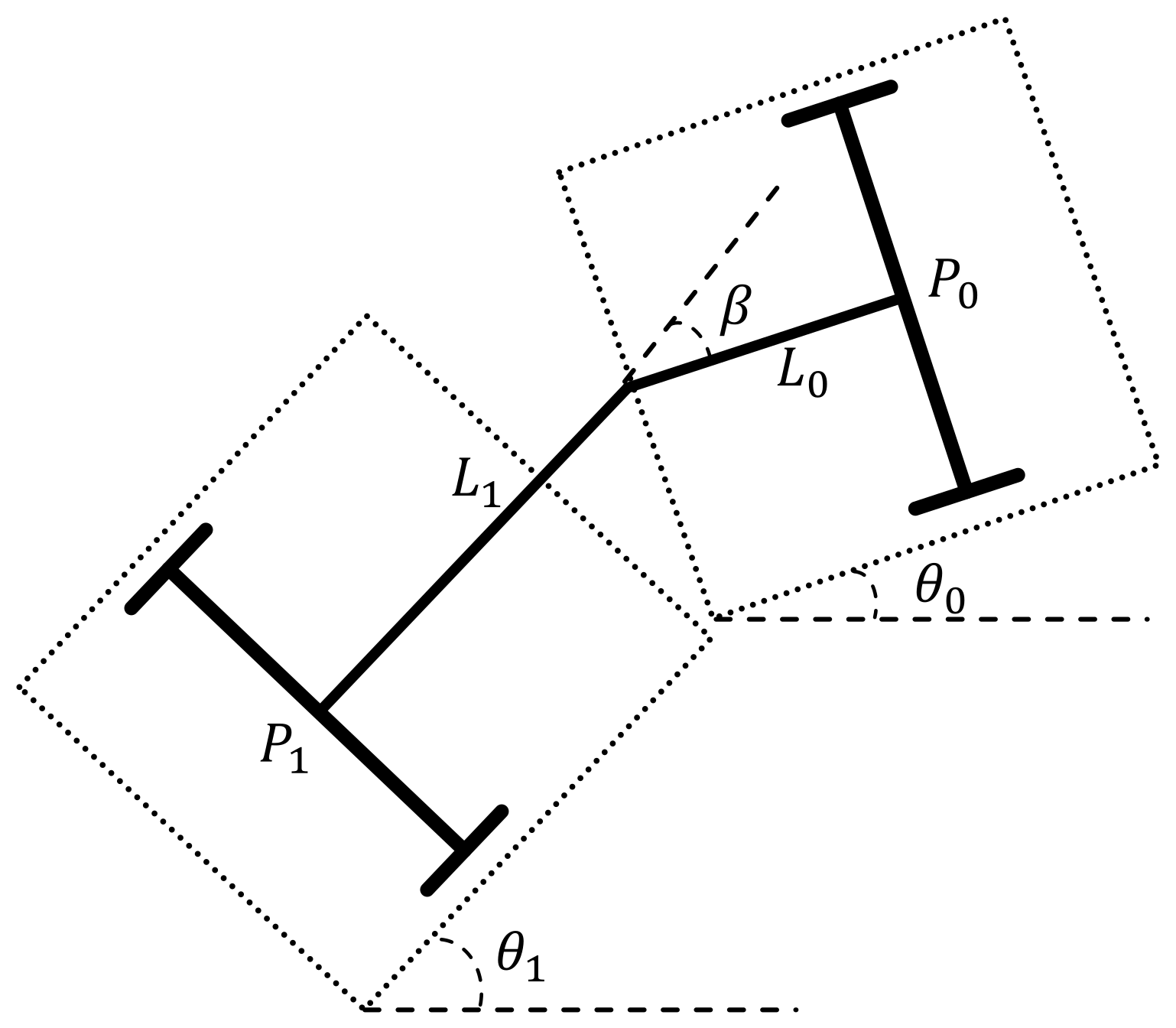
A multi-body point mass kinematic model is considered for both the front and rear chassis. The four rear wheels are combined to form a single axle at their midpoint. The coordinate frame of the truck model is given in
Figure 8 where
identifies the body,
is the midpoint of the axle given in Cartesian coordinates
,
is the orientation angle of the midpoint of the axle,
is the articulation angle,
is the velocity vector, and
is the distance between the axle midpoint and the articulation point.
The kinematic model of the rear chassis is then given by
and the front chassis, derived from the geometry of the truck, is given by
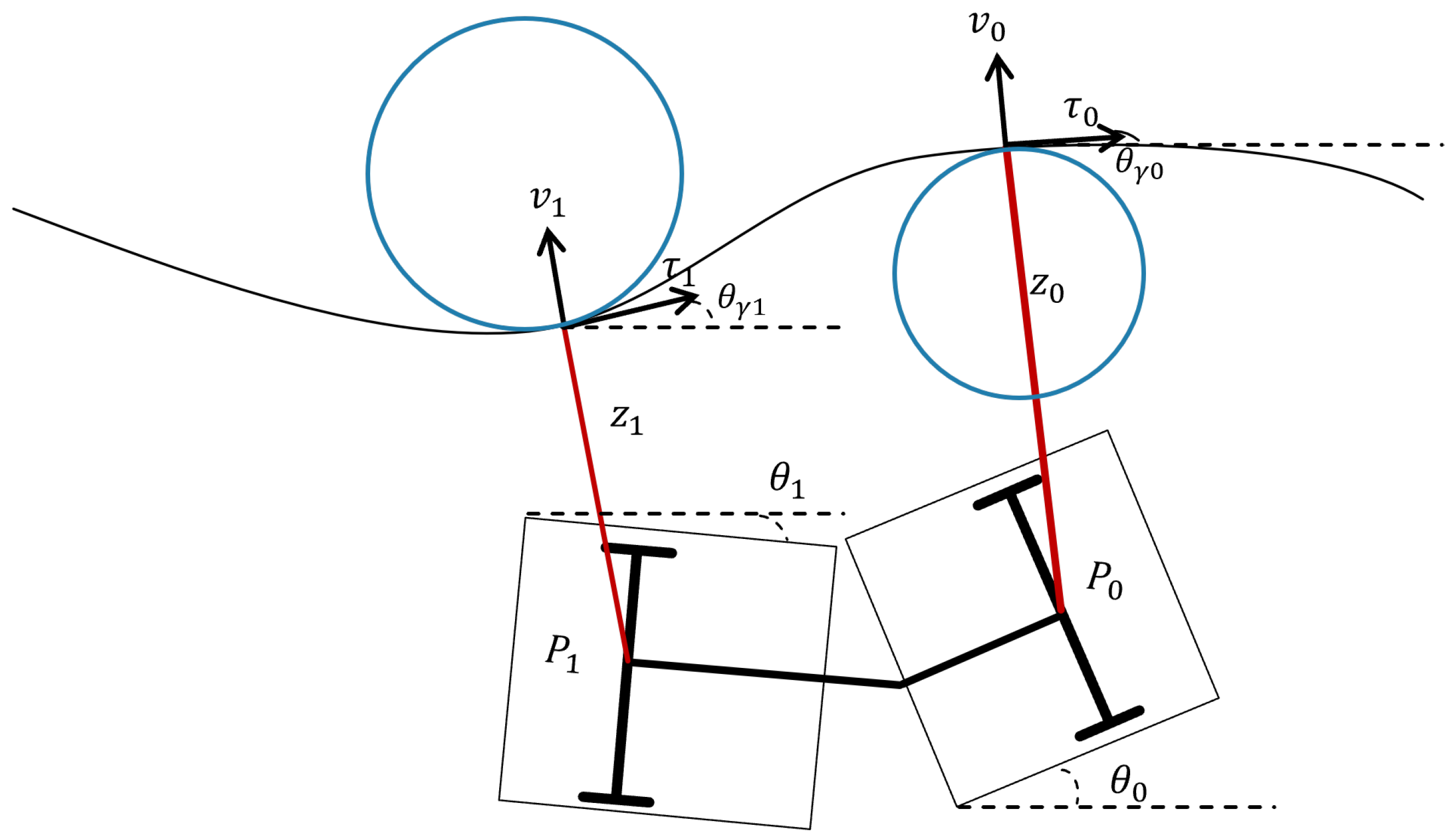
2.4.2. Path Tracking Criterion
The path tracking criterion was developed based on the path tracking criterion presented in [
17]. The midpoints of the front and rear vehicle bodies,
and
, are projected onto the path. These projections construct a Frenet frame. This provides a local representation of the vehicle bodies on the path. The underlying assumption is that the path is sufficiently smooth. The Frenet frame contains both a normal vector, which is the orthogonal distance of
from the path, and a tangent vector, which is the orientation of the path. This is shown in
Figure 9 where
is the orientation of the Frenet frame with respect to the inertial frame,
and
are the unit vectors of the normal and tangent to the curve respectively defining the Frenet frame, and
is the distance of point
from its orthogonal projection on the path.
It is important to consider the tracking of both the front and rear chassis to avoid collisions of the vehicle with its surroundings. Path tracking criterions based on a single guide point may not guarantee the orientation of both the front and rear chassis when following the path. Therefore, a path tracking criterion based on the offset of both chassis is considered and given below,
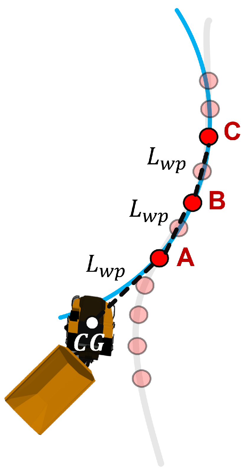
2.4.3. Circular Lookahead
The circular lookahead presented in [
14] allows the construction of a simple curve lookahead from three waypoints along the path. This type of lookahead accounts for the curve constraint of the path tracking criterion by guaranteeing a smooth curve between the fitted points. The circular lookahead proposed finds the closest waypoint on the path to the truck and moves along the path a minimum distance
to obtain three waypoints for the curve construction as shown in
Figure 10.
The minimum distance between the path waypoints considered for fitting,
, is dependent on the sampling rate of the controller,
and the velocity of the truck,
v,
Using this curve construction on both the front and rear bodies of the truck results in two circles that locally represent the path. The front and rear bodies can then be orthogonally projected onto these circles and the distance from the projection, , and the orientation of the truck on the path, , can be found.
2.4.4. Feedback Design
The state vector can be obtained from the dynamics of the points
in the Frenet frame as shown in [
17]. The state vector is given by,
and its dynamics,
where
is the relative orientation angle between the truck orientation and the path orientation,
is the curvature of the path, and
is the steering speed.
The dynamics of the state equation can be locally asymptotically stabilized to a path of constant curvature by linearization around the equilibrium and a linear state feedback as shown in [
17]. Since the path representation is already local, i.e. the circle fitting, then the constraint on asymptotic stability is met. For a path of constant curvature,
, the equilibrium point becomes,
that is obtained from the geometry of the path tracking problem in
Figure 9 and by imposing the path tracking criterion,
and setting the relative orientation angles,
to 0 at equilibrium. This is because the vehicle should move along a circumference concentric with the path at equilibrium. Note that the values of
and
result in a unique value for
.
Writing the system dynamics as
and taking the Jacobian of
A, denoted as
about the equilibrium point yields a Hurwitz matrix. Taking a linear state feedback for the control, the closed loop state matrix becomes,
where
K is selected as a feedback gain row vector to stabilize the closed loop system and
. This path tracking controller is capable of tracking in both the forward and reverse directions. The equations in this subsection along with the proofs are presented in [
17].
3. Results and Discussion
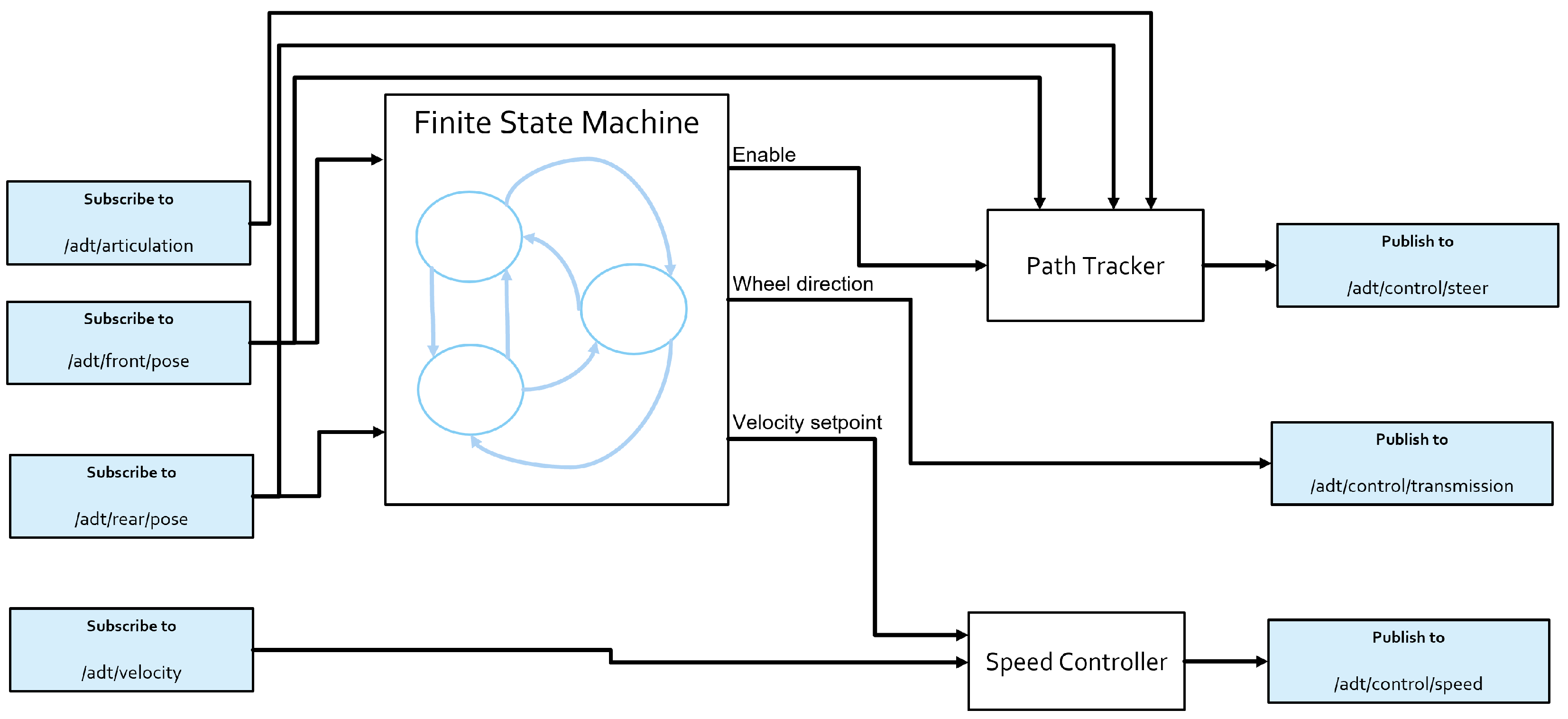
The FSM developed for the series of operations defined was used as the decision-making logic for the load-haul-dump operation. The Finite State Machine was constructed in Simulink and integrated with the path tracking module. The integration of the Finite State Machine with the path tracking controller in the simulation environment is outlined in
Figure 11. The finite state machine outputs setpoints or enable flags to the controllers based on the received information from simulation. The state transition events execute at each time step to determine the current state of the FSM.
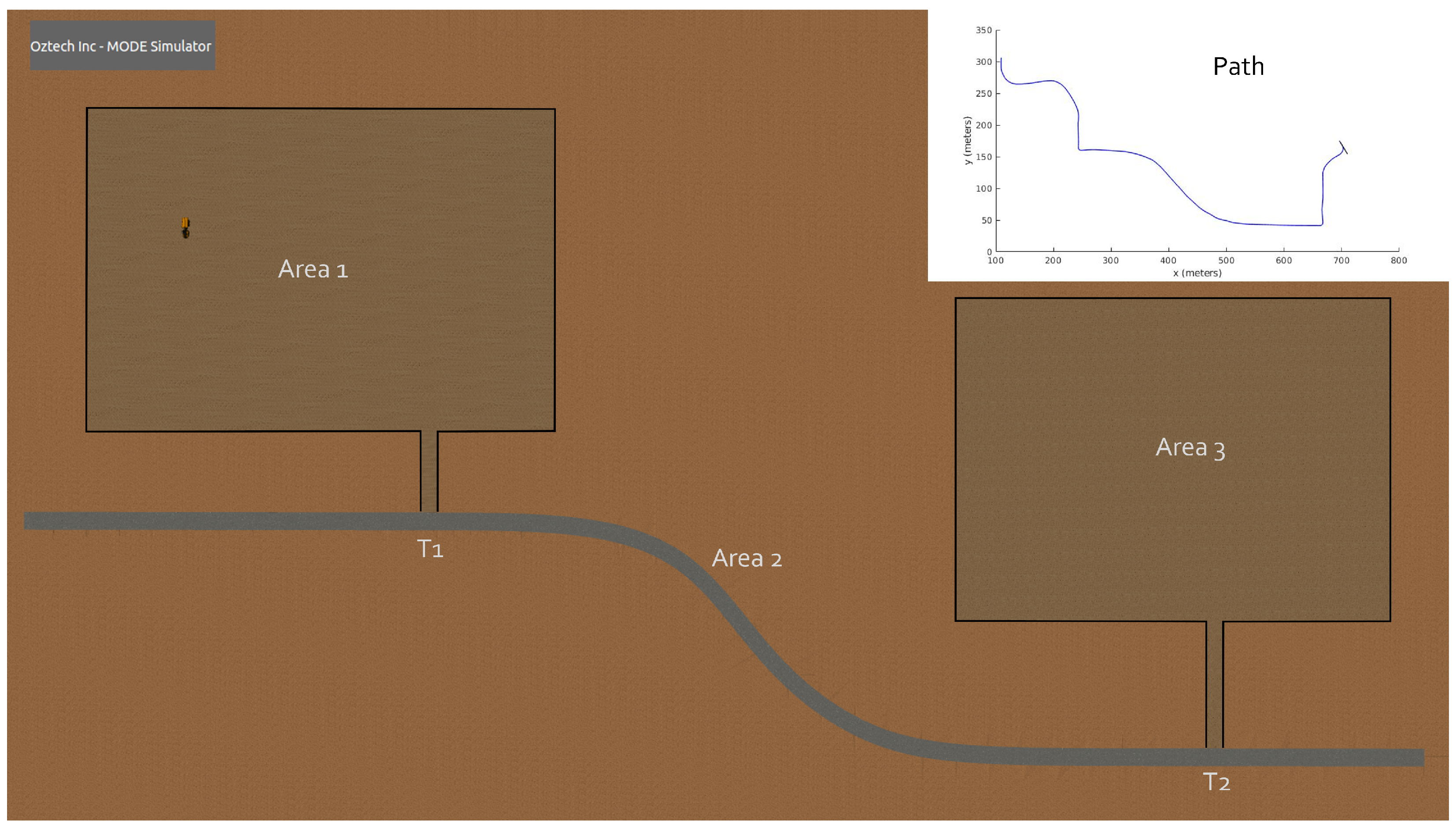
An example simulated scenario was constructed where the truck operation starts in A1 and ends in A3 and then reverses into the unload position. This represents stages 1 to 7 in the operational decomposition defined. A set of waypoints were collected and provided at the start of the simulation that define a path from A1 to A3. A simple PID speed controller was implemented to control the speed of the truck in the different areas. The scenario setup is shown in
Figure 12.
Figure 13,
Figure 14 and
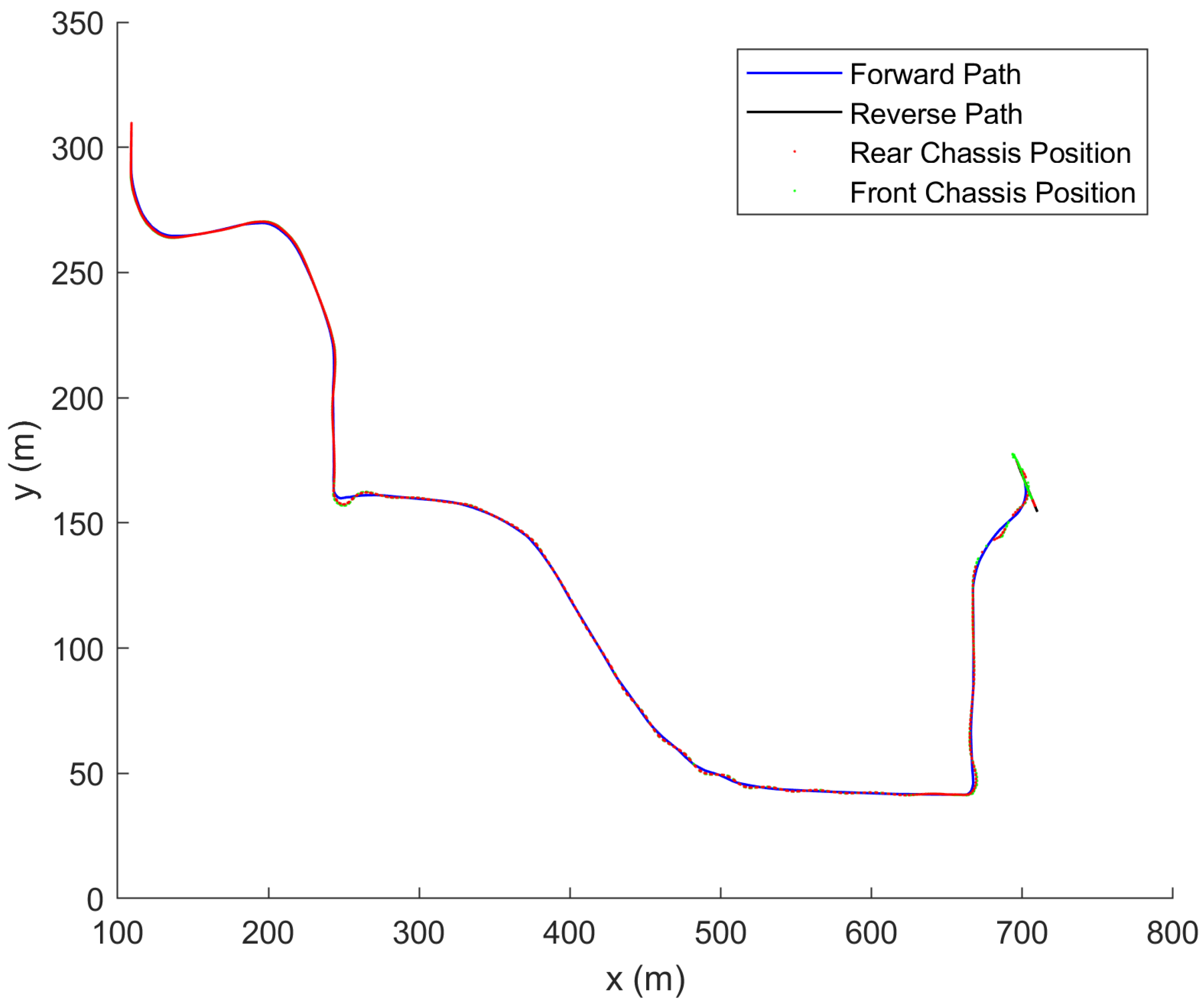
Figure 15 show the performance of the implemented module in the Oztech MODE simulator. The module was successful in tracking the provided path and performing a series of operations to move from A1 to A3—hence, complete a load-haul-dump operation. The last section in A3 represents a docking maneuver. The truck has to get into position and back into the unload position.
4. Conclusions
In this paper, a system architecture for the automation of the load-haul-dump operation of an articulated dump truck was proposed and tested in a physics-based 3D simulation environment. The proposed architecture was successful in performing the series of operations autonomously and demonstrating the effectiveness of this approach. While this paper provided an example of a surface mine and an articulated truck; this work can be easily extended to different vehicles, operations and layouts through proper operational decomposition. Moreover, this presents the core logic that can be extended to more complex tasks such as sensing, reactive obstacle avoidance, and other aspects that were not considered in this work but can be simulated using the presented physics-based simulation environment.
Author Contributions
Conceptualization, B.H. and U.O.; methodology, B.H. and U.O.; software, B.H.; validation, B.H.; formal analysis, B.H. and U.O.; investigation, B.H. and U.O.; resources, B.H. and U.O.; data curation, B.H.; writing—original draft preparation, B.H.; writing—review and editing, B.H. and U.O.; visualization, B.H.; supervision, U.O.; project administration, U.O. All authors have read and agreed to the published version of the manuscript.
Funding
This research was partially funded by Keisoku Giken Co, Yokohama, Japan.
Institutional Review Board Statement
Not applicable.
Informed Consent Statement
Not applicable.
Data Availability Statement
Not applicable.
Acknowledgments
The authors would like to thank Keisoku Giken Co. for the support.
Conflicts of Interest
The authors declare no conflict of interest.
Abbreviations
The following abbreviations are used in this manuscript:
| LHD | Load-haul-dump |
| ADT | Articulated dump truck |
| DES | Discrete event system |
| FSM | Finite state machine |
| GPS | Global Positioning System |
| ROS | Robot Operating System |
| MODE | Modular Design Environment |
References
- Hamada, T.; Saito, S. Autonomous haulage system for mining rationalization. Hitachi Rev. 2018, 67, 87–92. [Google Scholar]
- Komatsu, T.; Konno, Y.; Kiribayashi, S.; Nagatani, K.; Suzuki, T.; Ohno, K.; Suzuki, T.; Miyamoto, N.; Shibata, Y.; Asano, K. Autonomous driving of six-wheeled dump truck with a retrofitted robot. In Field and Service Robotics; Springer: Singapore, 2021; pp. 59–72. [Google Scholar]
- Gaber, T.; El Jazouli, Y.; Eldesouky, E.; Ali, A. Autonomous haulage systems in the mining industry: Cybersecurity, communication and safety issues and challenges. Electronics 2021, 10, 1357. [Google Scholar] [CrossRef]
- Brophey, D.; Euler, D. The Opti-Trak system, a system for automating today’s LHDs and trucks. CIM Bull. 1994, 87, 52–57. [Google Scholar]
- Duff, E.S.; Roberts, J.M. Wall following with constrained active contours. In Field and Service Robotics; Springer: Berlin/Heidelberg, Germany, 2003; pp. 51–60. [Google Scholar]
- Duff, E.S.; Roberts, J.M.; Corke, P.I. Automation of an underground mining vehicle using reactive navigation and opportunistic localization. In Proceedings of the 2003 IEEE/RSJ International Conference on Intelligent Robots and Systems (IROS 2003) (Cat. No. 03CH37453), Las Vegas, NV, USA, 27–31 October 2003; Volume 4, pp. 3775–3780. [Google Scholar]
- DeSantis, R. Modeling and Path-Tracking for a Load-Haul-Dump Mining Vehicle. J. Dyn. Syst. Meas. Control. 1997, 119, 40–47. [Google Scholar] [CrossRef]
- Alshaer, B.; Darabseh, T.; Alhanouti, M. Path planning, modeling and simulation of an autonomous articulated heavy construction machine performing a loading cycle. Appl. Math. Model. 2013, 37, 5315–5325. [Google Scholar] [CrossRef]
- Petrov, P.; Bigras, P. A practical approach to feedback path control for an articulated mining vehicle. In Proceedings of the 2001 IEEE/RSJ International Conference on Intelligent Robots and Systems, Expanding the Societal Role of Robotics in the the Next Millennium (Cat. No. 01CH37180), Maui, HI, USA, 29 October–3 November 2001; Volume 4, pp. 2258–2263. [Google Scholar]
- Bigras, P.; Petrov, P.; Wong, T. A LMI approach to feedback path control for an articulated mining vehicle. In Proceedings of the 7th International Conference on Modeling and Simulation of Electrical Machines, Converters and Systems, ELECTRIMACS, Montreal, QC, Canada, 18–21 August 2002. [Google Scholar]
- Dragt, B.; Camisani-Calzolari, F.; Craig, I. Modelling the dynamics of a Load-Haul-Dump vehicle. IFAC Proc. Vol. 2005, 38, 49–54. [Google Scholar] [CrossRef] [Green Version]
- Azizi, M.; Tarshizi, E. Autonomous control and navigation of a lab-scale underground mining haul truck using LiDAR sensor and triangulation-feasibility study. In Proceedings of the 2016 IEEE Industry Applications Society Annual Meeting, Portland, OR, USA, 2–6 October 2016; pp. 1–6. [Google Scholar]
- Challenge, D. Route Network Definition File (RNDF) and Mission Data File (MDF) Formats; Technical Report; Defense Advanced Research Projects Agency: Arlington County, WV, USA, 2007. [Google Scholar]
- Ozguner, U.; Acarman, T.; Redmill, K. Autonomous Ground Vehicles; Artech House: Norwood, MA, USA, 2011. [Google Scholar]
- Kurt, A.; Özgüner, Ü. Hierarchical finite state machines for autonomous mobile systems. Control. Eng. Pract. 2013, 21, 184–194. [Google Scholar] [CrossRef]
- Komatsu. HM300-5 Articulated Truck. Available online: https://www.komatsu.com/en/products/trucks/articulated-trucks/hm300-5 (accessed on 7 June 2021).
- Altafini, C. A Path-Tracking Criterion for an LHD Articulated Vehicle. Int. J. Robot. Res. 1999, 18, 435–441. [Google Scholar] [CrossRef]
Figure 1.
Road topology and operation of the load-haul-unload operation (top) and unload-haul-load operation (bottom). A1 represents the loading area, A3 represents the unloading area, and A2 represents the roadway connecting the loading/unloading areas. Waypoints are shown in red and checkpoints are shown in orange.
Figure 2.
Finite state machine logic for the operational decomposition of a load-haul-dump operation. E1 to E18 define the state transition events.
Figure 2.
Finite state machine logic for the operational decomposition of a load-haul-dump operation. E1 to E18 define the state transition events.
Figure 3.
Architecture of the Oztech MODE simulator. The environment consists of four main components: the simulated vehicle and world built on top of Gazebo, the 3D models, the control and communication interface through ROS, and the external scripts.
Figure 3.
Architecture of the Oztech MODE simulator. The environment consists of four main components: the simulated vehicle and world built on top of Gazebo, the 3D models, the control and communication interface through ROS, and the external scripts.
Figure 4.
Environment model of the operation description. Top-left area is the loading area while the middle-right area is the unloading area.
Figure 4.
Environment model of the operation description. Top-left area is the loading area while the middle-right area is the unloading area.
Figure 5.
Construction of the articulated truck model. (a) shows the rigid-body construction of the articulated dump truck. Suspension joints at the wheels were modeled as prismatic joints. (b) shows the articulated dump truck model in simulation.
Figure 5.
Construction of the articulated truck model. (a) shows the rigid-body construction of the articulated dump truck. Suspension joints at the wheels were modeled as prismatic joints. (b) shows the articulated dump truck model in simulation.
Figure 6.
Sensor view in rviz. The output of two LiDARs (red and blue) and the truck model is visualized.
Figure 6.
Sensor view in rviz. The output of two LiDARs (red and blue) and the truck model is visualized.
Figure 7.
Integration with MATLAB and Simulink.
Figure 7.
Integration with MATLAB and Simulink.
Figure 8.
Articulated truck model for kinematic modeling. Coordinate frames for the multibody decomposition of the articulated truck is shown.
Figure 8.
Articulated truck model for kinematic modeling. Coordinate frames for the multibody decomposition of the articulated truck is shown.
Figure 9.
Projection of the axle midpoints onto the path. The Frenet frames coordinate axes (, ) are also shown.
Figure 9.
Projection of the axle midpoints onto the path. The Frenet frames coordinate axes (, ) are also shown.
Figure 10.
Construction of the circular lookahead through three waypoints a minimum distance apart. The transparent waypoints represent the path and the highlighted waypoints represent the selected waypoints. The blue curve is the circle fitted through these waypoints.
Figure 10.
Construction of the circular lookahead through three waypoints a minimum distance apart. The transparent waypoints represent the path and the highlighted waypoints represent the selected waypoints. The blue curve is the circle fitted through these waypoints.
Figure 11.
Integration of the FSM and path tracking module in the simulator. The modules subscribe to the topics published by the simulated ADT and publish control commands to the control interface provided.
Figure 11.
Integration of the FSM and path tracking module in the simulator. The modules subscribe to the topics published by the simulated ADT and publish control commands to the control interface provided.
Figure 12.
Simulated scenario in Oztech MODE representing stages 1 to 7 of the operational decomposition. The reference path is constructed and shown on the top right.
Figure 12.
Simulated scenario in Oztech MODE representing stages 1 to 7 of the operational decomposition. The reference path is constructed and shown on the top right.
Figure 13.
Path tracking performance of the FSM and Path Tracking module in operating from A1 (load) to A3 (dock and unload).
Figure 13.
Path tracking performance of the FSM and Path Tracking module in operating from A1 (load) to A3 (dock and unload).
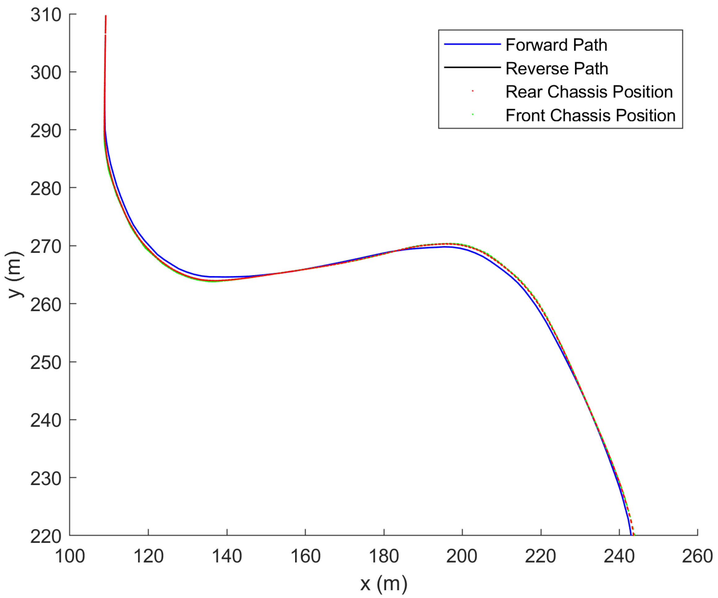
Figure 14.
Forward path tracking in A1. Blue line represents the path constructed from the waypoints. The red markers represent the GPS position of the front chassis read from the simulator.
Figure 14.
Forward path tracking in A1. Blue line represents the path constructed from the waypoints. The red markers represent the GPS position of the front chassis read from the simulator.
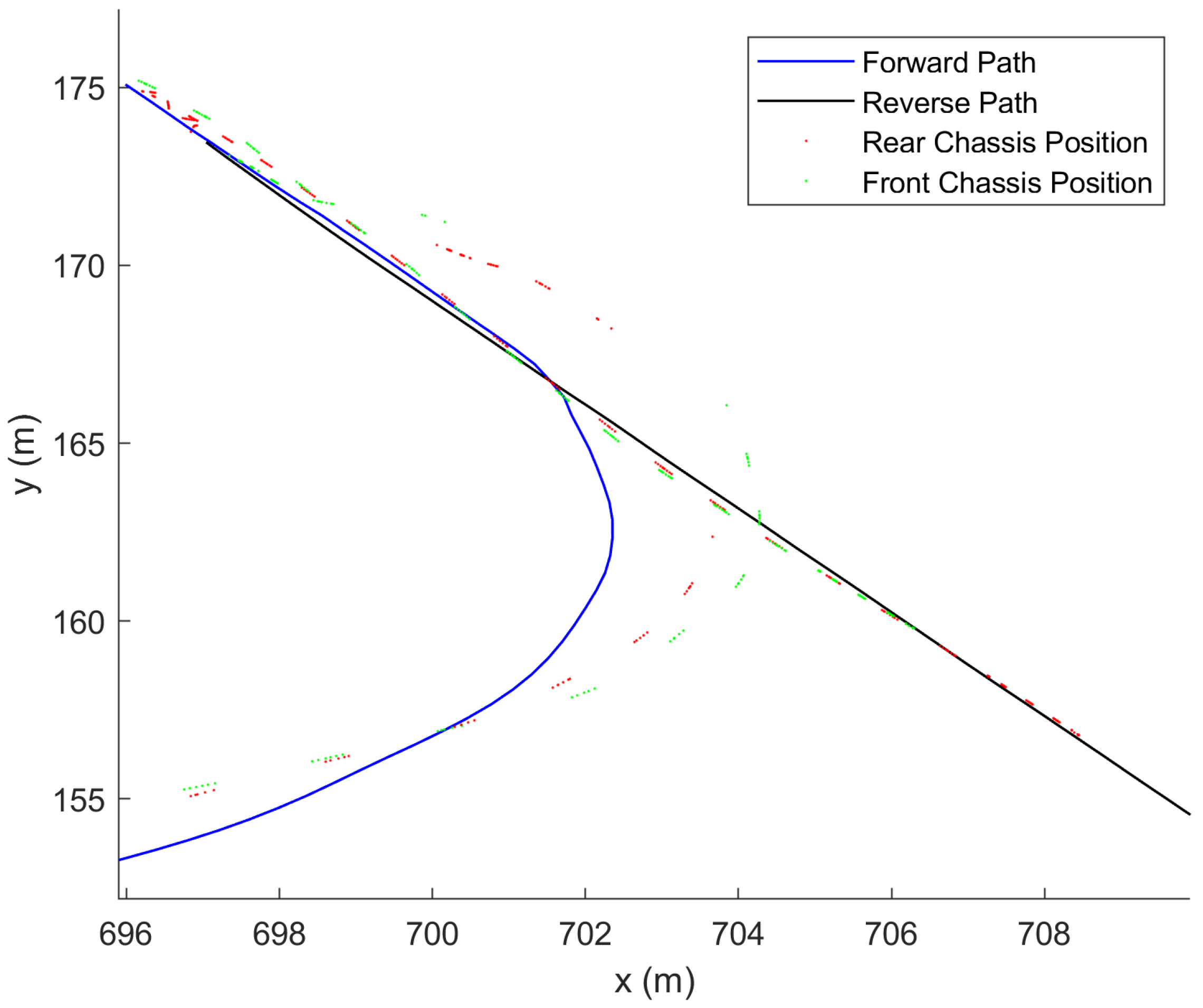
Figure 15.
Docking maneuver in A3. This maneuver includes both forward and reverse path tracking, the order of operations is decided by the FSM. Blue line represents the path constructed from the waypoints. The red markers represent the GPS position of the front chassis read from the simulator. Similarly, the green markers represent the rear chassis.
Table 1.
State transition events for the finite state machine logic developed for the operational decomposition.
Table 1.
State transition events for the finite state machine logic developed for the operational decomposition.
| Event | Condition |
|---|
| E1 | Truck position is in Area 2 (from Area 1) |
| E2 | Truck position is in Area 1 |
| E3 | Truck position is in Area 3 |
| E4 | Truck is in Area 2 (from Area 3) |
| E5 | Truck has been loaded |
| E6 | Truck is unloaded AND truck reached loading waypoint |
| E7 | Truck is loaded AND truck reached Area1-Area2 T-junction entry waypoint |
| E8 | Truck is unloaded AND truck reached Area2-Area1 T-junction exit waypoint |
| E9 | Truck is loaded AND truck reached Area1-Area2 T-junction exit waypoint |
| E10 | Truck is loaded AND truck is at Area1-Area2 T-junction
OR
Truck is unloaded AND truck is at Area2-Area3 T-junction |
| E11 | Truck is loaded AND truck reached Area2-Area3 T-junction entry waypoint
OR
Truck is unloaded AND truck reached Area2-Area1 T-junction entry waypoint |
| E12 | Truck reached Area2-Area3 T-junction exit waypoint
OR
Truck reached Area2-Area1 T-junction exit waypoint |
| E13 | Truck is loaded |
| E14 | Truck is unloaded and truck reached Area3-Area2 T-junction entry waypoint |
| E15 | Truck is loaded and truck reached backup waypoint location |
| E16 | Truck is loaded and truck reached the unload waypoint location |
| E17 | Truck has been unloaded |
| E18 | Truck is unloaded and truck reached Area3-Area2 T-junction exit waypoint |
| Publisher’s Note: MDPI stays neutral with regard to jurisdictional claims in published maps and institutional affiliations. |
© 2022 by the authors. Licensee MDPI, Basel, Switzerland. This article is an open access article distributed under the terms and conditions of the Creative Commons Attribution (CC BY) license (https://creativecommons.org/licenses/by/4.0/).


