An Approach for Robust System Testing the Event Data Recorder in the Context of a Passive Safety System

Abstract

As long as road accidents happen, passive safety systems like the airbag control unit are an essential part of the whole automotive safety system. Within the airbag control unit, the event data recorder (EDR) is an integrated function. Recent developments in legislation show that an increasing number of EDR-related regulations are being introduced. They are mainly focusing on data recording, crash-data retrieval, and some of them define testing aspects. In the system testing of an airbag control unit with a focus on the event data recorder, the question arises of how to deal with the fact that real-world crash events are not “straightforward” but arbitrary and do not follow any rules and restrictions. The purpose of this work is to develop a robust test approach to these conditions—giving a tester the possibility to extend the test depth considering the common test design techniques and testing principles. The applied methodology is the use of optimization algorithms in an automated test environment. With this, the tester can steer the test execution in a predefined way with minimal interaction. The application of the developed test method automatically creates a set of test data which fulfill the predefined conditions by the user. The generated results show that a high number of test data are created at and close to the target condition. Consequently, this test approach provides an extension to the common test design techniques with regard to how test input data can be created, and especially how automated test data creation and test execution can be realized.

1. Introduction and Background

Whenever an accident occurs and several parties are involved, the question of guilt arises. If there are eyewitnesses, they can be listened to. However, these reports are subjective and may be false. The national authorities counter this problem with the legal stipulation that vehicles must be equipped with an event data recorder (EDR) [1,2]. The purpose of the EDR is to objectively record accident data so that an accident reconstruction is subsequently supported by understanding “‘real-world’ crash dynamics and […] airbag deployments” [3] (p.1).

A continental approach to record crash data is realized as an integrated function of the airbag control unit (ACU) [4,5]—this function is called the “Event Data Recorder”. The ACU as a part of the passive safety systems has access to data prior to a crash event but also to those which are present during and after the crash. Therefore, the event data recording within an ACU has to cover a wide range of data within the different phases of an accident. 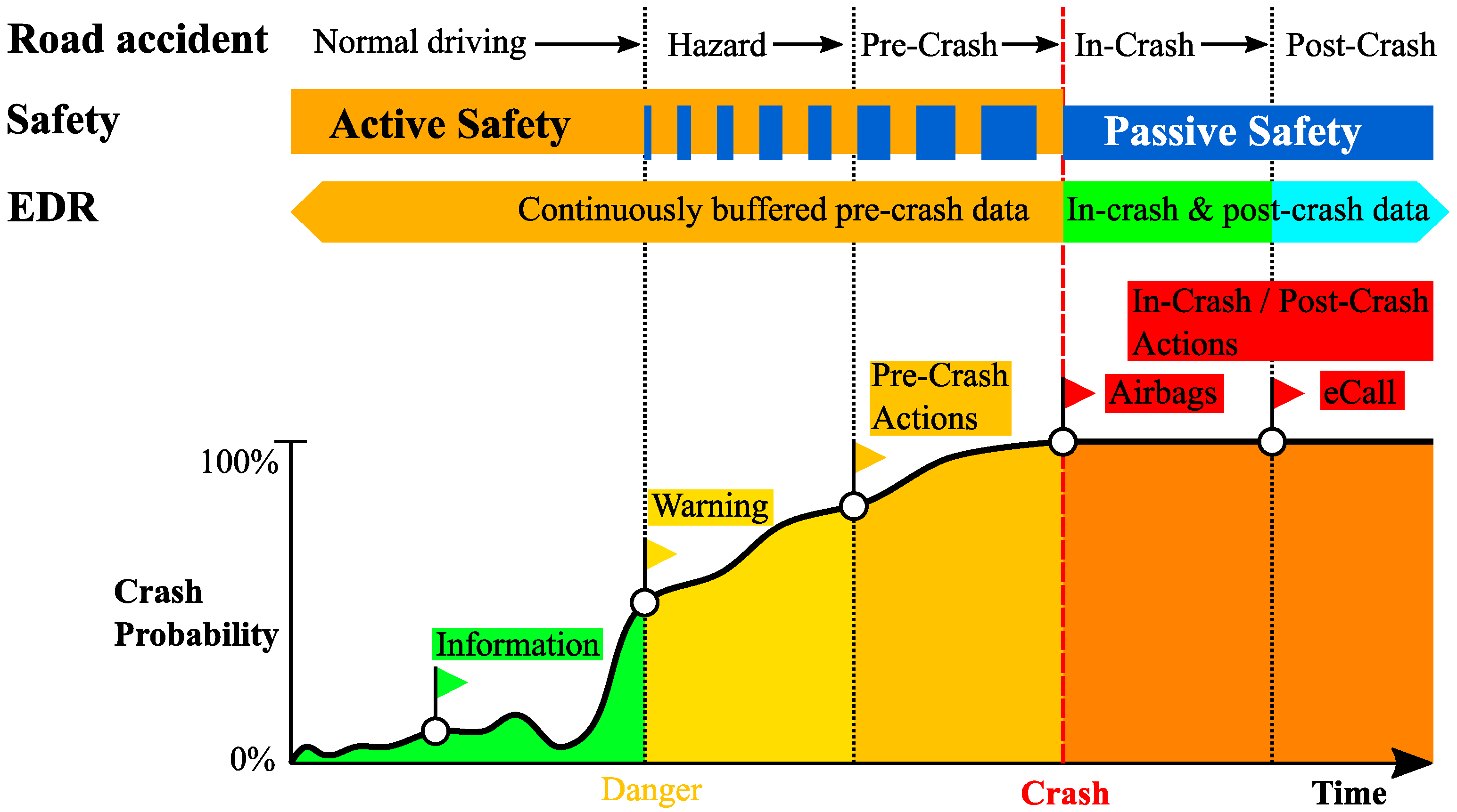Figure 1 shows, over time, that a road accident is divided into five phases:

• Normal driving;
• Hazard;
• Pre-Crash;
• In-Crash;
• Post-Crash.

It shows also that during the phases “hazard” and “pre-crash”, there is an overlap of active safety and passive safety. This means that passive safety does not begin only at the point in time when a crash is happening but can act also already in the case of a present hazard. For example, the activation of belt pre-tensioners can be triggered by i.e., a driving maneuver before crash occurrence and even without a crash event [6].

For crash data reconstruction, and the event data recorder, this example shows that various aspects have to be considered like the trigger of an event record and the content of the record itself.

For system testing (=black-box testing) the test execution is performed only accessing the external interfaces of a device under test [7,8], here the airbag control unit. Therefore, testing the EDR function implies testing the airbag control unit as a whole. The standard test approach is to derive test cases from requirements, analyze and vary input data or i.e., perform experience-based testing. The main aim of this work is to develop a robust test method for how to perform EDR testing additionally to the standard test approach. It focuses on the goal of system testing to ensure that the EDR always records the correct accident history data completely and in compliance with the law. Requirements from the regulations describe the expected behavior of the EDR and their coverage is mandatory. The complexity to be considered for the EDR is that it must be able to record any theoretically possible accident history—no matter how many previous events have occurred that met the condition but were subsequently discarded. If an accident occurs in which an airbag is deployed, this event must be reliably and completely stored in the EDR. Considering all field scenarios, the combinatorics of events become arbitrarily complex. To achieve maximum test coverage, the EDR must theoretically be verified with all accident sequences possible in real road traffic. An attempt to provide the complete dynamics of the real accident sequences as test input data is doomed to failure right from the start and cannot be realized in series development for reasons of time alone. This is one of the testing principles as they are defined in [9] (“exhaustive testing is impossible”). In order to perform effective testing, two additional testing principles must be considered—the “pesticide paradox” and “defects cluster together”. These two principles state that repetition of the same tests might be ineffective if they do not find any new unexpected behavior (“pesticide paradox”), and that if one defect was found the probability is high that other defects exist in the same function (“defects cluster together”). This results in the following challenges. On the one hand, if one defect occurred, the test must search for additional defects close to the condition of the obtained defect. On the other hand, the test has to stay effective and must not perform same tests again and again if no new defects are found. The application of these testing principles on testing the EDR is extended for the following case. Not only are defects a matter of interest. The regulations define various requirements, i.e., towards timely behavior, performance and data storage. These requirements can be mapped to either the input or the output data since they are describing them. For system testing, this means that two formats must be considered—the crash signals representing the EDR input data and the EDR entry as output data. For example, due to a defect it might be necessary to test focused on a dedicated critical timing and expected behavior. Knowing that a “defect cluster” might exist, it is of interest to perform tests also close to the critical timing. In order to automate such tests, a relation between input and output data must be established. With the help of suitable methods, this relation can be formulated as a mathematical optimization problem. Methods like genetic algorithms or particle swarm optimization are suitable to solve such optimization problems [10,11,12]. All of them follow a common approach. A target state (i.e., defect) defines a search-space for the optimization. The optimization itself is performed iteratively, using either a pre-defined starting point or a random starting point. The evaluation of an optimization loop is undertaken via the fitness function which provides a fitness value—the proximity to the target state. With this, an automated, iterative test data creation is introduced which is applicable in functional testing.

Solving optimization problems by using i.e., evolutionary algorithms is an established method and can be applied in different scenarios [13]. In the automotive context, various studies have been published—in [14], the functions adaptive cruise control (ACC) and active emergency brake system (AEB) were tested using evolutionary algorithms. For the ACC, the fitness function used data of vehicle motion, restrictive conditions (like minimum distance to vehicle in front or max. deceleration) and driver interaction (steering, braking). A similar approach was used for the testing of the AEB. Environmental conditions like curve radius, radar data and vehicle motion, were used within the fitness function. In both cases, the fitness function was formulated using the input format of the device under test. In [6], differential evolution methods have been used for testing the activation of reversible restraints. Similar to [14], the input format of the fitness value calculation is equal to the input format of the device under test (or tested function). Also, in [15] an automated parking system is tested using evolutionary algorithms. All these studies have in common that the test scope is a function which can be analyzed analytical i.e., using kinematic motion equations or, more general, following physical laws such as minimum distance to driving vehicle in front, a critical point until a crash cannot be avoided (having all physical values available); or, as with the park assistant, where critical points/values can be derived based on the equations of motions and assumed trajectory.

By contrast with these studies, here the purpose of the EDR testing is to ensure the law-compliant behavior of this function. Since these laws and regulations are man-made, one of the main challenges is to define an adequate fitness function which allows quantification of (partly) qualitative information which does not follow physical laws. This is realized by using the output format of the device under test (EDR function) for the fitness value calculation.

2. Materials and Methods

Regulations define which data must be recorded in the event of an accident and how an EDR record has to be stored. This work deals with the latter, recording the accident history itself. For the EDR, there are three relevant criteria for this; the start time of the record, the decision whether to save or discard the ongoing record, and finally the end time of the recording. At the start time, the EDR freezes the continuously buffered data, the so-called pre-crash data. Subsequently, the EDR records additional information, such as deployment decisions. This corresponds to the in-crash and post-crash data. If a deploy decision is made, this event shall be stored. If no deployment decision is made and the start condition is also no longer fulfilled, the current event is not worth recording and must be discarded. The recording interval of the post-crash data is defined by law [1,2] and thus determines the end time. A detailed perspective shall be given in Figure 2. It shows the timeline of the phases of an accident (see Figure 1) up to the crash data analysis. Aligned with these phases, it visualizes the data provided by the corresponding actor.

Beginning with normal driving up to post-crash, the event data recording stores various information related to the vehicle motion itself, i.e., accelerations and angular rates, but also occupant status information, i.e., buckle switch state and passenger airbag deactivation status [1,2]. The properties (recording interval, accuracy, …) and format (values, unit, data length, data position, …) of these so-called “data elements” is pre-defined by the standards, too [1,2,16]. With these definitions, the bit and byte-coded data elements stored in an airbag control unit can be read out using a commercial data retrieval tool. This tool interprets the coded data and provides it in a human readable format which can be used for crash data analysis; see for example a Tesla EDR record in [17]. Also, BOSCH provides a crash data retrieval (CDR) tool, where the latest software can be downloaded at [18].

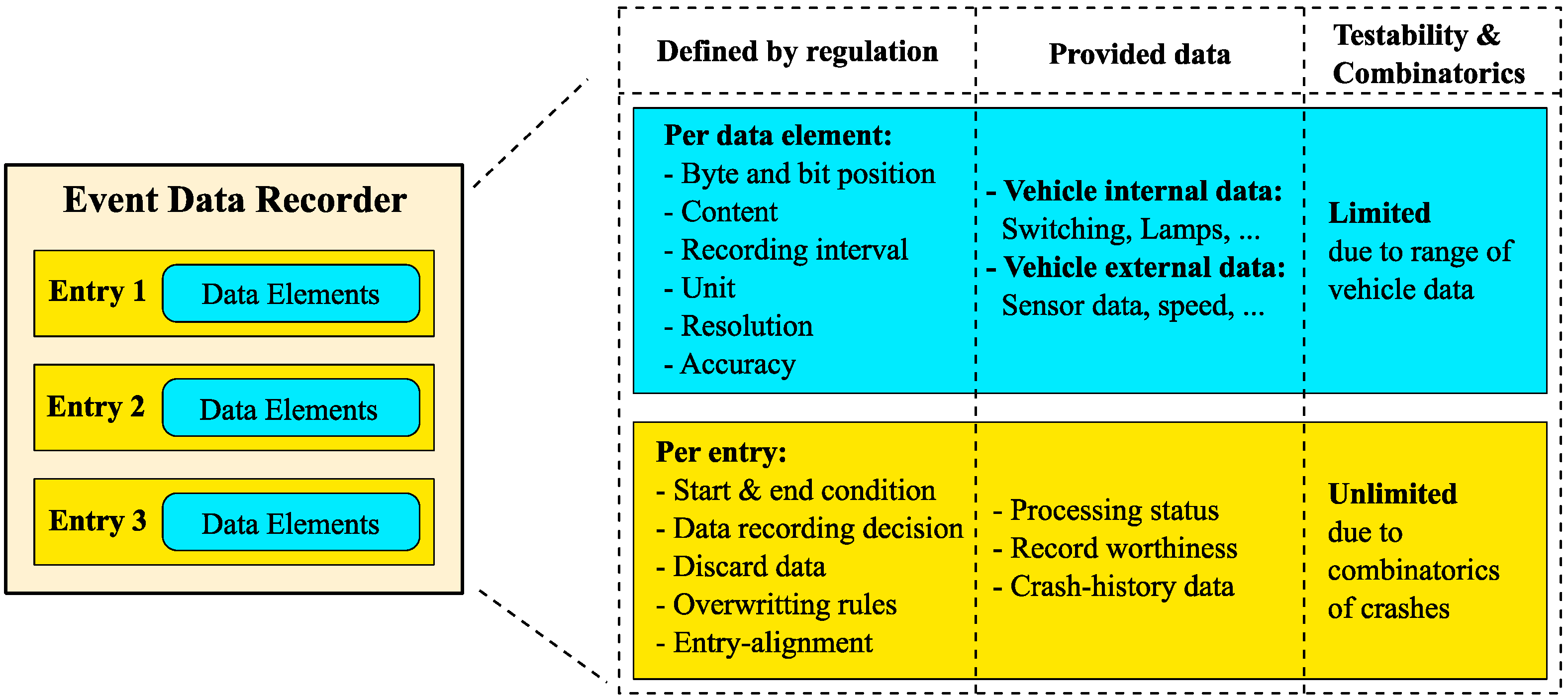
The data elements themselves are encapsulated in the so-called “EDR Event Entry”, see Figure 3. For the handling of the EDR event entries, dedicated requirements exist [1,2]. The legislation of the National Highway Traffic Safety Administration (NHTSA) and China Automotive Technology and Research Center (CATARC) are defining the start conditions of an EDR event, when a started event recording has to be stored and also rules how to discard or overwrite events [1,2]. These requirements deal with the fact that crash events are not singular events which happen once but that various combinations may appear depending on the event type. For this, the legislation states that it must be possible to store at least two [1] or three [2] EDR events.

The three columns on the right side of Figure 3 are showing what the regulations are defining, which data is provided with respect to the data elements (blue) and EDR event entry (yellow) and the testability in terms of combinatorics. Referring to the data elements, various properties are defined like which states of a buckle switch have to be recorded or the range and resolution of an acceleration signal. For the event entries, the handling of the recording is described—trigger conditions, data recording and rules when to overwrite or discard events. Additionally, it contains the information of the processing status and, taking all available EDR entries into consideration, a crash-history can be determined (because of the existing rules how to record, overwrite or discard events). For testing, the combinatorics per data element is limited due to the limited range of available inputs and data properties. In contrast to this, the combinatorics of recording event entries can be judged as unlimited. This is because the event entries are reflecting the crash-history data and there are unlimited scenarios possible when it comes to reflect real-world crash scenarios.

2.1. Handling of Event Data Recorder (EDR) Event Entries

Focusing on the recording of an EDR event entry, the main items to be considered are:

• Start condition;
• The decision to either store or discard an ongoing event record;
• Whether an already stored event has to be overwritten.

An exemplary mapping of crash activity to EDR state is given in Figure 4. It shows the mapping of measured acceleration and the derived airbag algorithm state and EDR activity states. The EDR event may be triggered by wake-up algorithms or by reaching a cumulative delta-V threshold, whichever appears first [1]. This is mapped to the EDR activity state “Event Start”.

The purpose of the given example is to illustrate how the crash progress—represented by the acceleration—is interconnected with the EDR activity states. Here, the airbag algorithm state “wake-up” is triggering the EDR event start (time zero t₀). Also, it is possible that the cumulative delta-V triggers the EDR event start. However, whether the event has to be recorded or not is depending on the deploy decision of the airbag algorithm. The end of an event is, again, depending on the algorithm state (reset) and the cumulative delta-V [1]. For the purpose of easier visualization, in the following sections of this work only the EDR activity states are displayed—the general behavior is as described in Figure 4.

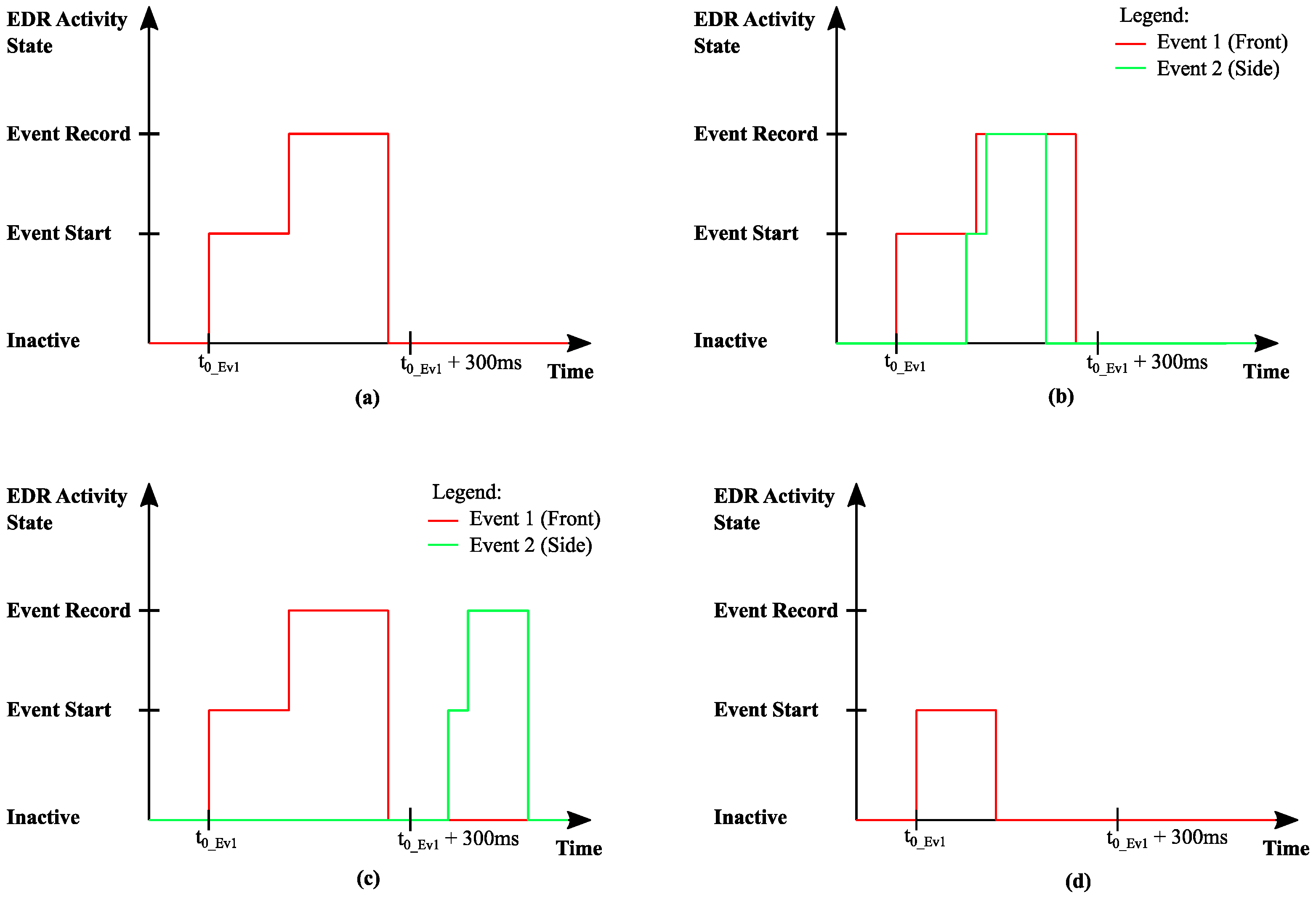
An overview about possible EDR activity states and the occurrence of multiple events is provided in Figure 5. Here, four EDR event classifications are introduced:

(a)

Single event;

(b)

Parallel event

(c)

Multi event

(d)

Trivial event.

In case 1, it shows that only one event is taking place. The maximum recording interval is 300 ms after the event starts [1,2]. Once it is decided to record the event, the recording takes place at a maximum up to 300 ms after the event starts. In case 2, for easier understanding, the differentiation of event 1 and event 2 as front or side event is introduced. It shows that a second event is started after the start of the first event and that the second event ends earlier than the first event—the second event is encapsulated by the first event. 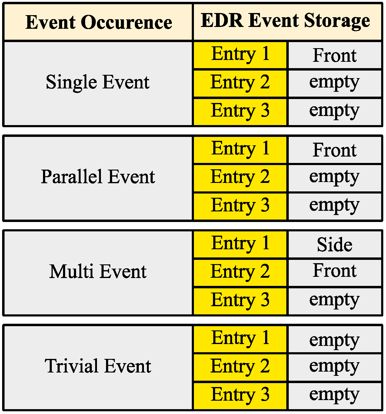This is called a parallel event and the EDR recording of such an event’s occurrence follows pre-defined rules [1,2]. Same applies for case 3. The events themselves are the same as in (b), they are only shifted in a timely manner, so that the second event begins after the first event has already ended but within 5 sec after the start of the first event. This is called a multi event. Finally, case 4 shows that only an event start took place followed by the state “inactive”. This means, that any condition was met to start the event but no record decision was made (record worthiness was not present). All the front and side events shown (besides case 4), are equal. They are only different in their timely occurrence. The impact of this timing on the EDR event storage is visualized in Figure 6.

From the EDR storage perspective, cases 1 and 2 are similar. Only one event is stored—parallel events can be stored as only one event [16]. Case 3, the multi events, are stored individually [1]. Finally, case 4 is not stored at all. Trivial events are triggering an EDR event start and freeze the pre-crash data but they are discarded. To be complete, it has to be mentioned that also a “lock state” is existing. Unlocked events could be crash events with deployment of reversible actuators or triggered via the delta-V threshold of 8 kph within 150 ms [1,2]. The overwriting rules for EDR event entries, as mentioned in Figure 3, are applying mainly for unlocked events since locked events are not overwritable [1,2]. Besides this, the locked and unlocked events are handled in a similar way.

2.2. Testability of the EDR Event Handling

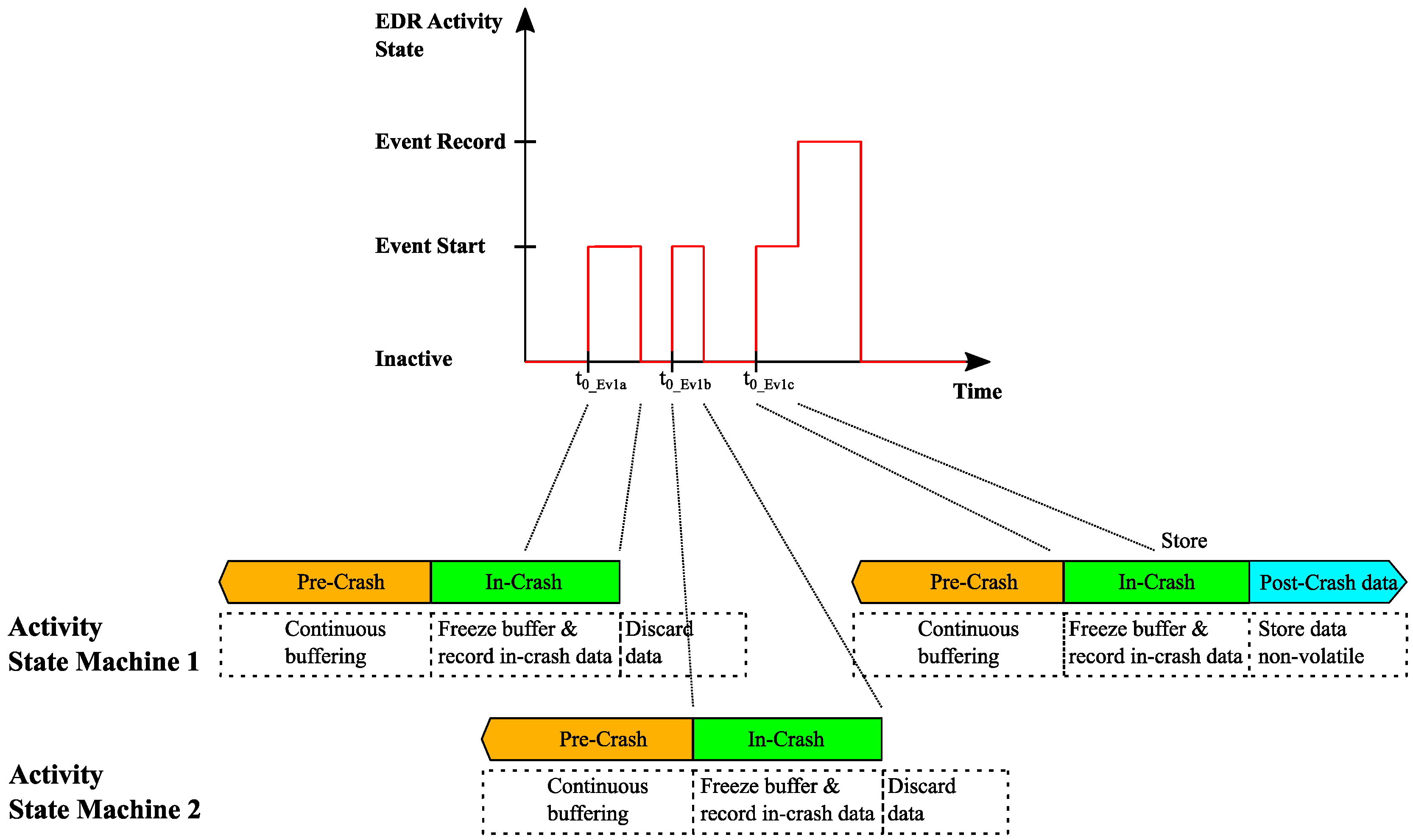
In Figure 5 and Figure 6, some examples have been given of how EDR activity scenarios and recorded EDR event entries are handled. In order to explain the testability, the example of a single event with one or more trivial events in front shall be given. Trivial events are triggering the EDR recording process because the start condition was met. However, no recording decision takes place and, therefore, this ongoing event recording has to be discarded. An example of what such an event can look like is given in Figure 7.

The event start condition is met two times without a recording decision. A third event (Event 1c) takes place which is worth to record. This means for testing that not only the recorded event has to be in focus but also the time history of prior events which fulfilled any of the start conditions but have been discarded. The reason why this is important is that each time a start condition is fulfilled, the continuously buffered pre-crash data are frozen and a state-machine is occupied. The fact that it is not possible to implement an infinite number of state-machines leads to the conflict of availability of state-machines and ongoing events. The following Figure 8 gives an exaggerated view of the relation between ongoing events within a dedicated timeframe and number of available state-machines.

The first state-machine freezes the buffered pre-crash data and is prepared to record in-crash and post-crash data. However, this ongoing event is not recorded, and the data are discarded. As long as this is ongoing, a second event start condition is met and the pre-crash data are frozen by the second state-machine. Again, this event is not recorded and, now, both state-machines can have an overlapping timeframe where the state-machines are still occupied with discarding the data or collecting the required buffer length of pre-crash data. The consecutive third event is recorded and stored. The EDR event storage will show only this third event. From EDR perspective it will not be visible that two prior events have been present. This example shows that the four different cases (see Figure 5) cannot be handled independently of each other. Only by applying combinations of various scenarios is it possible to get closer to a real-world crash scenario. One theoretical approach would be to create all combinations which are possible. This brute-force method is doomed to fail simply because of available time since there is no clear end-criteria when “all combinations” is reached. In the mentioned example, this leads to questions like:

• “How many previous trivial events shall be present?”
• “How long should the event(s) last?”
• “What is the time between the trivial event and the recorded event?”
• “Are, in case of more than one trivial event, all characteristics of these events equal or is each trivial event individual?”

Instead of taking these (and more) questions and trying to create special test cases manually, the aim of this work is to develop an automated and robust test approach which provides a systematic way to test the EDR considering these questions.

3. Formulation of the Hypothesis

After decades of testing, common experiences have been documented [9]. The International Software Testing Qualifications Board (ISTQB) defines in its syllabus for the “Certified Tester Foundation Level” seven testing principles [9]:

• Testing shows the presence of defects, not their absence;
• Exhaustive testing is impossible;
• Early testing saves time and money;
• Defects cluster together;
• Beware of the pesticide paradox;
• Testing is context dependent;
• Absence-of-errors is a fallacy.

In the context of this work, especially numbers 2, 4 and 5 are considered. Knowing that “exhaustive testing is impossible”, the focus in developing a test approach is an appropriate consideration of “defects cluster together” and “beware of the pesticide paradox”. In other words, since it is not possible to test all combinations, a “steering” of the test execution in the “correct” direction has to be ensured. The testing principle 4 gives guidance of how the test execution can be focused. If one defect was found at a certain condition it is most likely that additional defects are present but not yet found (=“defects cluster together”). Testing principle 5 gives another perspective on test execution. In the case of repeating test execution which does not find any new defects test cases or test data (=combinations) have to be changed. The term “pesticide paradox” is used analogously to the application of pesticides on insects while the insects already have an immunity and the pesticides are not effective anymore [9]. In [19], some robustness testing techniques are described. The developed test approach is applicable to cover—by the method itself—the use of random inputs, invalid inputs, physical faults and type-specific tests. This leads to the following working hypothesis:

Hypothesis 1 (H1).

The test-depth of an EDR can be increased by using a method to define dedicated target states and, at the same time, not giving any restriction how these states can be achieved. This extends the common test design techniques like boundary-value analysis or equivalence class partitioning. The search-space is not directly limited on a pre-defined range as it is the case i.e., for boundary-value analysis. It allows a controlled and flexible limit definition giving a wider range. With this, testing principle 4 is considered by the definition of a target state, and not giving restrictions on how to realize approaches testing principle 5. Finally, the realization of this method fulfills—by the test method itself—various criteria for a robust test technique.

First, an example for the application of the common test design techniques will be presented. Then, the hypothesis and test approach and how it extends the scope of the common test design techniques will be explained. In Figure 9, a comparison is made with respect to the search-space from the application of a boundary-value analysis, how the working hypothesis extends the search-space and, especially, why the extension is made.

In Figure 9a, an EDR parallel event is shown—a side event is completely embedded within an ongoing front event. Therefore, the application of a boundary value analysis is of interest. This leads to two search spaces. Search-space 1 defines which event occurs first. Search-space 2 defines the latest point in time for having overlapping events. In Figure 9b, two potential scenarios are derived how the application could be realized. The side event with the solid line shows the case that the side event is starting prior to the front event. The side event with the dashed line shows the case that the events are not overlapping anymore. The impact of these two potential scenarios is, in terms of EDR, that overlapping events are following dedicated requirements as to how such an event occurrence is handled with the EDR recording—whether overlapping events are handled as “one EDR event” and stored within one EDR event entry or if they are handled individually and stored in individual entries, e.g., following the requirements for multi-events. An overview of potential scenarios for Figure 9a,b is given in

Table 1. Potential scenarios derived from Figure 9a.

Scenario	Start Time of Side Event	Shown in Figure 9 As
1	t0_Ev1 + Δt	Solid line of (a) 1
2	t0_Ev1 − Δt	Solid line of (b)
3	tend_Ev1 + Δt	Dashed line of (b)
4	tend_Ev1 − Δt	Solid line of (a) 1

¹ From EDR event handling perspective, the handling is equal. These scenarios are duplicates and could be reduced to only one scenario, using the equivalence class partitioning method.

.

Focusing on only the event handling with respect to starting times, the test execution of only three scenarios would be sufficient to provide a basic coverage. Applying the general rules of equivalence class partitioning—all events of the same type with the same properties (start time conditions) have the same behavior [20]—leads to the fact that each scenario can be represented by only one test. Nevertheless, the goal of a tester is to test as much and as good as possible (considering the given constraints like available time). For the precise formulation of what this means, the testing principles have to be taken into account.

The hypothesis is that the test coverage can be increased (compared to the common test design techniques) by defining a wider range of a search-space and to steer the test data creation in an automated test environment. The “steering” of test data creation is covering especially the testing principles of the pesticide paradox and the defects cluster. Since there is no restriction at which the condition a defect might occur, the search-space is enlarged in order to cover all EDR activity states (compared to Figure 9). The following Figure 10 shows how in this working hypothesis the search-space is defined and how a potential application of the testing principles can be realized.

The search-space is enlarged and covers in the timely dimension a range that can be defined by the tester (t_val1 and t_val2 in Figure 10a). In the dimension of the EDR activity state, it covers all available states. In Figure 10b, the application in the context of the pesticide paradox has the same focus as the boundary-value analysis in Figure 9—the testing is focused on parallel events—but its realization can look completely different. In this example, all shown scenarios are parallel events, but they have completely different properties. Here, it is visualized as different times between the states “event start” and “event record”. In terms of the “pesticide paradox”, the same functional content is tested but the test data are different. In Figure 10c, the application in the context of defects cluster is detached from the previous use case—a search-space is defined close to t_{End_Ev1}. A typical test scenario in this case is that a defect was already found in a similar condition. Therefore, the search-space is formulated in a way that the condition of a known defect can be reproduced and fulfilled. Additionally, independent from the presence of defects, this approach can be used to define a search-space based on the outcome of an analysis (i.e., software function calls, performance, etc.).

4. Realization of the Test Approach

The realization of the developed test approach in an automated test environment depends basically on two items. First, how to realize the automated test execution itself and second, how to “steer” the test execution towards the target.

4.1. Preparation for Automated Test Execution

Performing test execution automatically, the following two topics have to be defined:

• A way to formulate how a required event scenario shall look like.
• A way to identify whether the required event scenario is achieved or not.

In order to formulate the required event scenario, the question arises as to which format the data shall be formulated in. The EDR itself records various data like speed signal, accelerations (longitudinal and lateral) and angular rates. The storage of an EDR record is, however, in a pre-defined way, storing bits and bytes following various rules. In this work, the input for the test execution is formulated in the format of an EDR record. This allows a target state to be formulated (simply said, the way an event shall look like) directly in the terminology of EDR. In the following text, this will be called “target EDR data”.

The identification of whether the desired event scenario is achieved indicates that it must be possible not only to make a direct comparison of an as-is state and the expected state but also to identify “how far away” is the as-is state from the target. Then, to get closer to the target state, it must be possible to steer the creation of the test data in a way that a newly generated data is closer to the target than the previous data. This implies already that this process is iterative and covers a progress from a starting point to the pre-defined target. This describes the basics for a mathematical optimization problem. For this, various approaches exist how optimization problems can be solved. In this work, the genetic algorithm is used.

4.2. Application of an Optimization Algorithm

Mandatory in the application and solving of an optimization problem is to create a proper fitness function. If the fitness function is developed wrongly or is not effective, the runtime to solve the optimization problem might be very high or the problem remains unsolved (since the fitness function steers the optimization loops towards the target). In [14], a method of structural testing and how a fitness function may be formulated accordingly are described. The following Figure 11 illustrates how the fitness function is developed and how it interacts with the required EDR event scenario.

Based on the mandatory properties of an event, the “target EDR data” are defined. The structural graph illustrates the design of the fitness function. This graph is not mandatory but supports the creation of the code of the fitness function. Here, a pseudo code shows how the fitness value is calculated. In general, it identifies the proximity of the as-is state to the target. In an automated environment, the fitness value is calculated per iteration. Potential progress of how the fitness value evolution over iterations may look like is shown in Figure 11d. This figure shows that the fitness function is realized using only EDR terminology (=the output format of the system)—it is independent from the test input data.

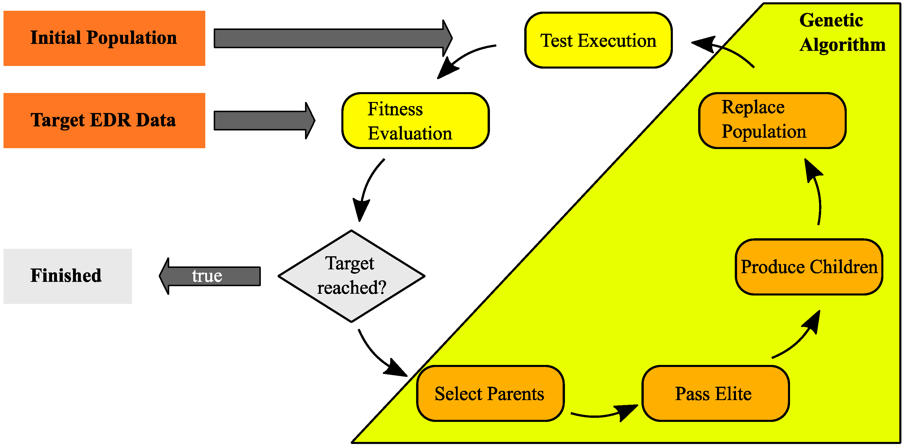
The general process of the application of an optimization algorithm is shown in Figure 12.

The initial population can be created randomly or by an individual selection of the user. After test execution, the test results are evaluated within the fitness function. If the target is reached, the optimization loop stops. If the target is not reached, the phases of the genetic algorithms are passed over until a new population is created and is available for the testing and the iteration starts from the beginning. In the context of this work, the optimization algorithm is used with the purpose of being a tool that allows iterative test data creation. It is not in the focus to investigate further algorithms such as particle swarm optimization or the techniques of simulated annealing to solve an optimization problem.

The automated test execution using an optimization algorithm may be realized in different ways. Figure 13 provides an overview about the interaction of the tester with the test environment, which test environments are identified and available in the context of this work and how the result evaluation may be realized. Special focus is on the optimization algorithm. Here, this algorithm serves as a kind of test controller. Because the input and realization of the fitness function is in the same format as the execution results, no separated test controller, parser or similar is required. The optimization algorithm is capable of iteratively generating test data which stimulates the system until the system behavior is equal to the “target EDR data” defined by the user.

In general, two kinds of test environment exist but three options exist as to how they can be combined. In option A, test execution is possible using only the hardware-in-the-loop (HiL) environment. In option B, additionally to the HiL execution a parallel model-in-the-loop (MiL) execution is possible. With this, additionally to the “real system”-results also simulation results are available. Here, the benefit is that the simulation model can be designed as an idealized model, e.g., having more EDR record entries available than in the real system. In option C, the HiL and MiL test executions are performed sequentially. The major benefit of this case is a reduced test execution time in the HiL environment. The initial execution in the MiL environment generates a set of test input data which fulfills the “target EDR data”-reached condition. In general, all created test input data can be stored and made available. With this, the tester can select test scenarios, i.e., “only target reached data”, and execute HiL tests using exclusively these data (= classical automated test execution, independent from the optimization algorithm). This sequence allows to separate the phases of “data creation” and “test execution with the real system”. Additionally, the option C is the best suitable test environment in terms of developing and improving the application of the optimization algorithm due to the short execution time.

For the flexible application of same test data within different test environments it has to be considered that the input format of the test environments might differ. Here, the HiL testing uses the test data input format of the airbag control unit. The MiL environment, however, does not simulate the complete airbag control unit. It focuses on the EDR function itself. As indicated in Figure 4, environmental vehicle data like accelerations and angular rates can be mapped to control unit internal states like the airbag algorithm states which, again, are used by the EDR. With this mapping, the same test data generated by the optimization algorithm can be used within different test environments.

5. Results and Discussion

The main aspect of the developed method with respect to automated execution is to create iteratively new test input data. Therefore, the results are created using the MiL environment (see also option C in Figure 13). The main aims of the developed test method itself are to approach the “pesticide paradox” as well as the “defects cluster”, see also Figure 9. For this, the following two cases are applied and investigated:

• Case 1—Single event with a trivial event in front:
  This case has a special focus on the “pesticide paradox”. In Section 2.2. about the testability of the EDR event handling, several questions are raised as to how to deal with a trivial event. Here, the “target EDR data” is formulated as having a single event duration of 210 ms and any kind of single trivial event in front. With this, a target is given for the single event itself, but no restrictions are given for the characteristics of the trivial event—how long it may last and its timely distance to the single event.

• Case 2—Parallel event where the end of the second event is 10 ms or closer to the end of the initial (starting) event:
  This case shall represent an assumed “defect cluster” close to the event end of a parallel event, as long as parallel activities are ongoing.

For the interpretation of the presented results it has to be considered that the target of an optimization loop is to create test input data which leads to an EDR event equal to the defined “target EDR data”. Therefore, the presented results will show the airbag algorithm state over time. For the mapping of EDR activities, airbag algorithm states and input data of the system see Figure 4. With this, a functional behavior of the EDR is always represented as the time behavior of the airbag algorithm states. For the purpose of easier visualization and focusing on the test method itself, the given examples are depending only on the airbag algorithm states—the cumulative delta-V was always set to values which do not influence the EDR event handling.

The parameter settings for the application of the genetic algorithm are shown in

Table 2. Overview of parameter settings of the genetic algorithm and the results.

Case	Population Size	Variable Parameters	Lower Limit	Upper Limit	Executed Generations 1	Generation—First Time Target Reached	Populations with Target Reached
1: Single Event	150	5	0 s	1 s	20	7	997
2: Parallel Event	150	6	0 s	1 s	19 1	14	266

¹ In this case a stall generation limit was activated.

.

The main parameters as the number of population size and limits are kept equal for both cases. The maximum number of generations was set in both cases to 20, but for case 2 a stall generation limit was activated (as an instrument to limit the run time of the optimization loops).

5.1. Single Event with Trivial Event

The target of this case is to create a trivial event with a subsequent single event. Mandatory for the automated test execution using an optimization algorithm is to define a target EDR state. In this case, the trivial event itself underlies no restrictions. This means that the trivial event itself does not have any “target” defined. The target EDR state is, however, described as the single event to be ending between 208 ms and 210 ms after the event start. Figure 14 shows the evolution of the fitness value over generations. Already after one generation, the best fitness value is zero. The target value of the fitness function (=−1) is reached for the first time after 6 generations. Here, no stall limit is activated—the optimization loop is continued even if the target value of the fitness function was already reached. Special focus is on the testing principle 5 (pesticide paradox). This means that the goal of these test executions is actually to create a lot of test data under defined conditions (at “target reached”). In the context of the pesticide paradox, beginning with generation seven, relevant test data are created.

The search-space, represented as fitness values, is divided into two sections. First, fitness values greater than zero indicate that test data are created which do not pass the plausibility checks. For instance, one basic check is that the created test data are triggering an event recording itself. Another example, more specific for this case 1, is to check that the created trivial event does not overlap with the single event (which would cause that no trivial event is present). The second section, fitness values between zero and minus one, indicates that test data are created which fulfill the criteria for a trivial event and a single event. In this case, the optimization loop is now steered towards the target condition of the single event. Even if the number of generations is not equally distributed between both search-spaces, the gradient of the fitness values provides an indication for the evolution steps over generations. In the first section, fitness values greater than zero, the gradient is positive and negative. This can be interpreted as a high distribution of the population, test data are created in “all directions” in order to find the most fitting values. In the second section, fitness values between zero and minus one, the gradient is always negative—the fitness value is monotonically decreasing and starting with generation 18, the fitness value seems to start converging. In this section, a lot of test data are created which all fulfill the same functional conditions.

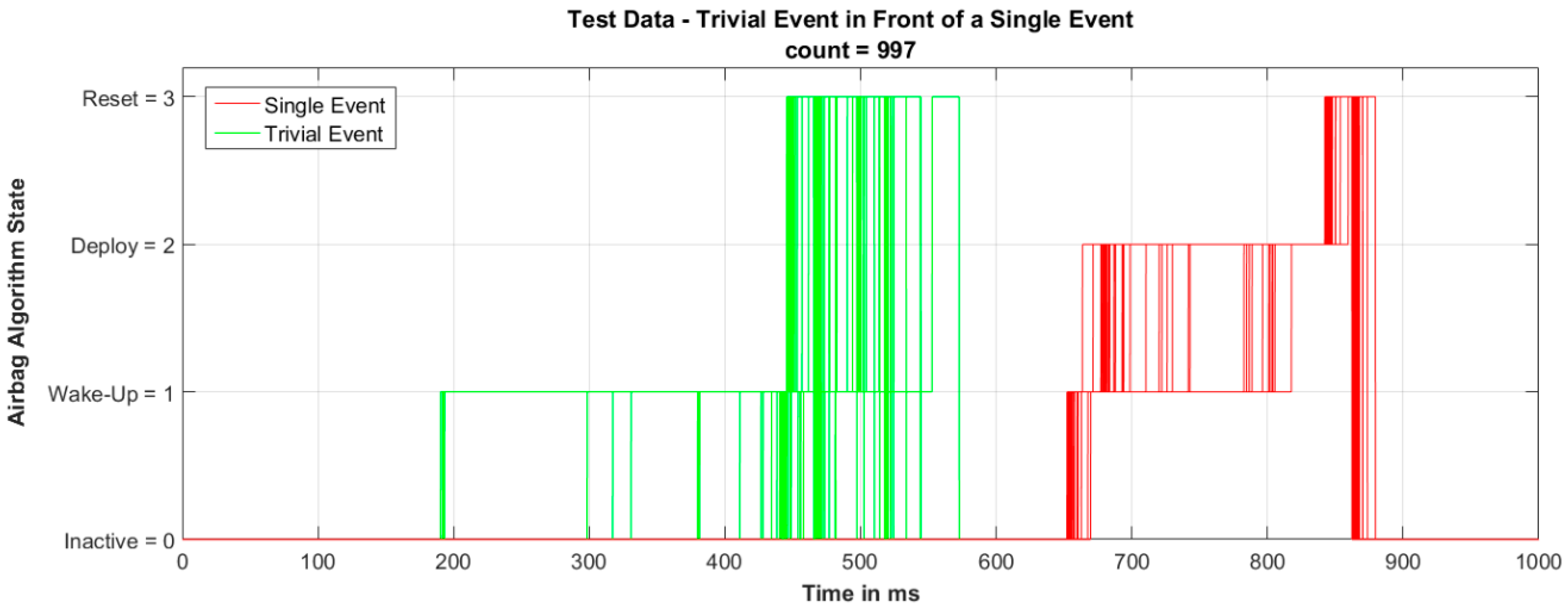
Figure 15 displays all generated test input data where the condition “target reached: fitness value = −1” is fulfilled—all these data are matching the “target EDR data”. The green line visualizes the trivial event. The red line represents the single event.

The generated single event does not vary much in its timing—clusters of “event start” (=wake-up) and “event end” (=transition from reset to inactive) for the single event are present. The high degree of similarity is expected because the optimization loop has steered the created test data towards these time values. By contrast with this, the created trivial events have a wide range. They differ in their “event start” as well as in the “event end” times. Also this is as expected because the trivial event does not underlie any restriction how the event has to be realized (from timely point of view).

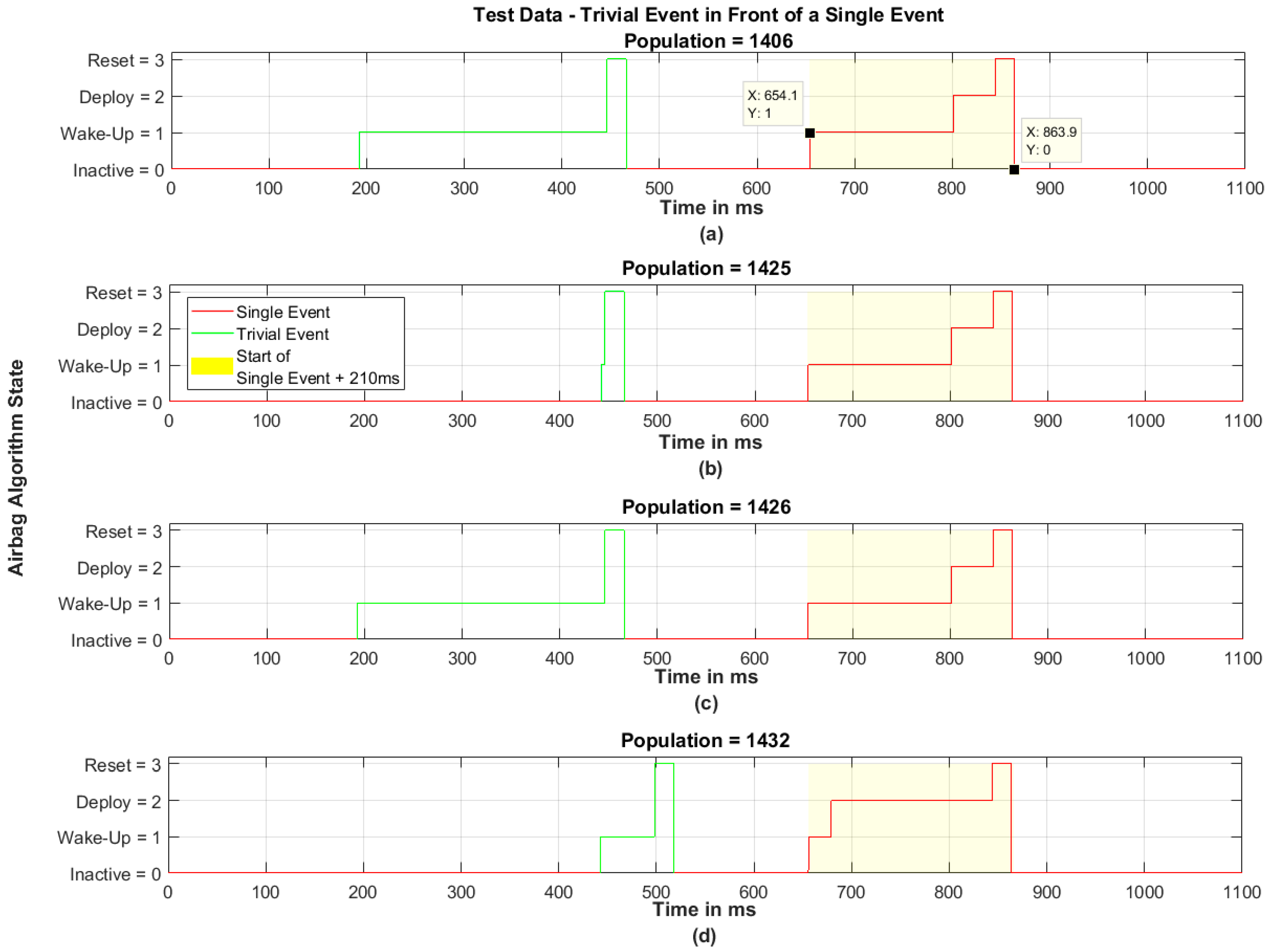
Figure 16 shows a detailed view of four created data sets at different populations. For example, one pair of data tips is added to show the timely characteristics.

These four subplots show that each created single event is, in terms of start and end condition, almost equal. The recording decision, however, is varying. The trivial events of the populations 1406 and 1426 are similar but completely different to the populations 1425 and 1432. The time between the end of the trivial event and start of the single event varies, from approx. 460 ms to 520 ms, as well as the duration of the trivial event itself. The range is from very short (population 1425) up to approximately 260 ms (populations 1406 and 1426).

5.2. Parallel Event

The target of this case is that the encapsulated event is ending less or equal to 10 ms before the initial event ends. The user selects a front event as the initial event and a side event as the encapsulated, parallel event. Figure 17 shows the progress of the fitness values over the generations. It shows that the target value of “−1” is reached at generation 14 the first time. Considering the population size, this means that the target was reached after a minimum 1950 iterations. In this optimization loop, a stall generation limit was activated and set to 5. After six consecutive generations with the same fitness value the optimization loop is aborted (generation count = first occurrence + five stall generations). Therefore, the optimization loop is stopped here at generation 19.

Like case 1, the search-space is divided into two sections. The first section is defined by fitness values between 1 and 7 and focuses on the plausibility check of created test data. In this special case, one plausibility check is to ensure that the created test data fulfill the conditions for a parallel event. Next to the timely behavior, this includes the condition that the user-selected event occurs first. The second section represents values between 1 and −1. Here, the fitness values between 0 and 1 are considered as “close to the target”. By contrast with case 1, the gradient of the fitness values is monotonically decreasing for all generations.

Because in case 2 the number of required generations until “target reached” is significantly higher than in case 1 (first “target reached” at generation 7), in Figure 18, a histogram of the fitness values is visualized for the condition “close to the target” (=fitness value between 0 and 1). This histogram shows that two major cluster are existing with a high population count. At fitness values of approximately 0.7 more than 200 populations are present and at fitness values of approximately 0.4 almost 150 populations. Additionally, two minor cluster with a little number of populations exist at fitness values of approximately 0.3 and 0.7.

This histogram also shows the tendency of increasing number of populations as the fitness value gets closer to the target. Generally, this is expected because the optimization algorithm evolves the population to the fittest values.

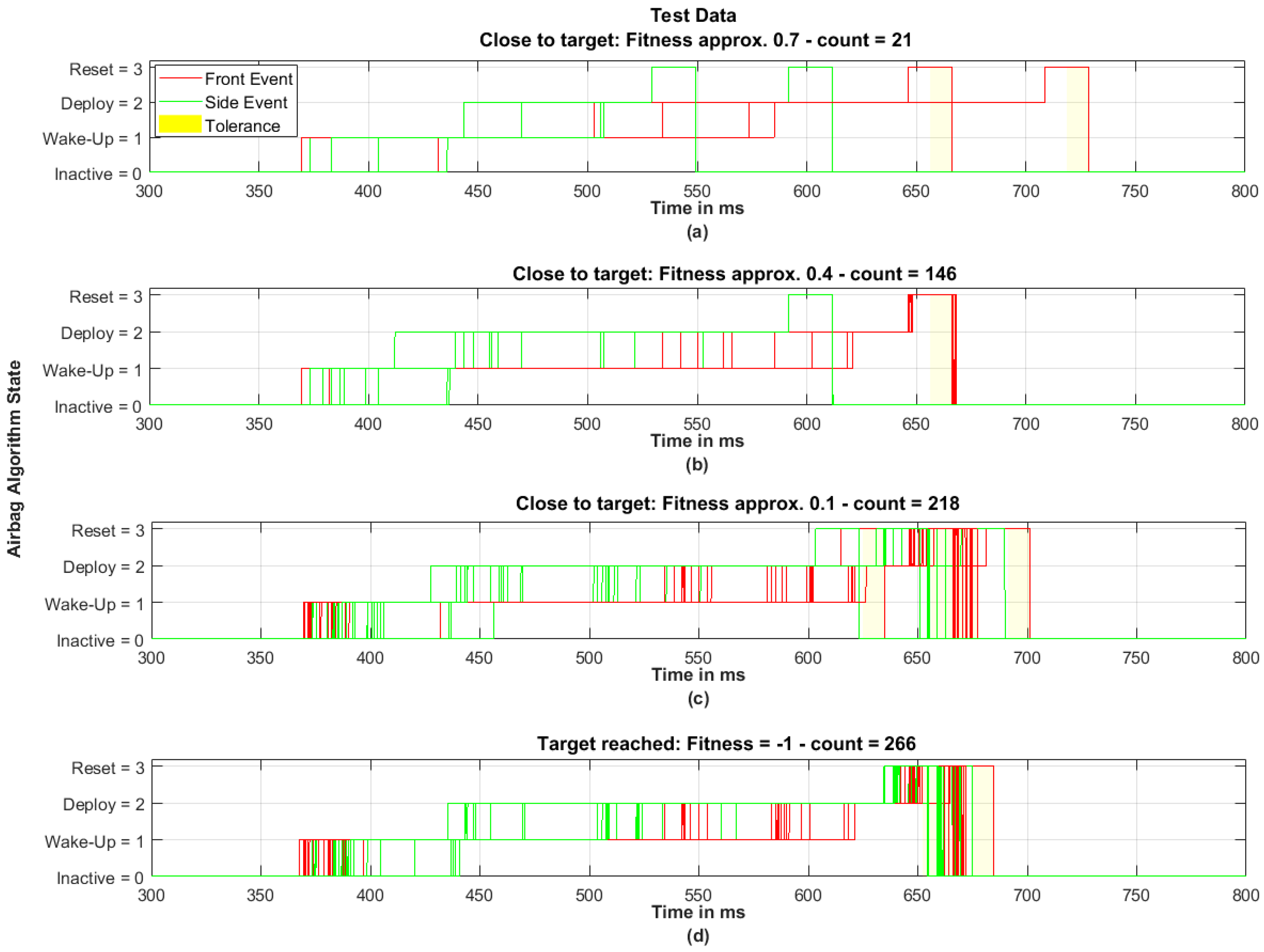
Figure 19 shows in subplots the evolution of test data reaching the target value. The three subplots Figure 19a to Figure 19c are showing selected cluster as indicated in Figure 18. The Figure 19d shows the test data at the condition “target reached”. At each falling edge of the “reset”, a tolerance band is highlighted. In case the end of the second event (side) is inside this tolerance band, the fitness function would respond “target reached”—it does not show which pair of “front event” and “side event” belong together. Therefore, as in Figure 19c (target value 0.1), some side events seem to be located within the tolerance band but are not considered as “target reached”. This means their corresponding front event data set has an event end distance of more than 10 ms.

The Figure 19a shows test data for the fitness values at approximately 0.7. Although the plot seems to show a very little number of created test data, only two falling edges of the front event can be obtained, the count is 21. Similar behavior occurs for the start condition and, in total, for the side event. This indicates that the created test data with respect to start and end conditions are either identical or very similar (which is visualized as identical in the given resolution). Figure 19b displays test data for the fitness values at approximately 0.4. Again, only a small number of front start conditions can be obtained, and all event end conditions of the front event are close to 670 ms. The side event, however, shows the presence of various start conditions in a range of approximately 80 ms but only one falling edge at approximately 610 ms. In Figure 19c, test data with fitness values at approximately 0.1 do show that all start conditions of the front event are in a time window of 360 ms to 390 ms and almost all event end conditions occur between 660 ms and 680 ms. Similar behavior occurs for the side event. The start and end conditions show clusters while the deploy decision is varying in a wide range (compared to the range of the start and end conditions). The Figure 19d shows only test data at the condition “target reached”. In direct comparison with Figure 19c above with respect to the front event, both plots seem to be very similar (besides the falling edge in Figure 19c at 700 ms). In particular, with these two subplots the effect of the optimization loop can be obtained. All end conditions of the side event are inside the tolerance band at the end condition of the front event. It is expected that the end of the side event is evolving from far to close to the end of the front event because the optimization loop is targeting the timely difference between these two event end conditions. Additionally, the results of all these subplots show that the optimization algorithm has created test data for the front event with end conditions at 700 ms (Figure 19c) and at 730 ms (Figure 19a) which have been considered as “close to the target”, too. Although Figure 19a indicates an equal distribution of test data with front event end at 670 and 730 ms, populations with a front event end at 700 ms or later did not survive in the optimization algorithm.

6. Conclusions and Future Work

Performing system tests of the EDR as an integrated function of the airbag control unit shows that the test execution cannot be performed by stimulating the EDR directly. The stimulus is always applied on the external interface of the system. In the presented test approach, a method was introduced to show how the focus can be set more encapsulated on the EDR function itself by using the environmental conditions of the EDR event handling—which are represented by the airbag algorithm states and the cumulated delta-V. The goal of systematically extended automated test execution is reached by the application of an optimization algorithm. The genetic algorithm itself serves as a tool to iteratively create new test input data. Defining the “target EDR state” and formulating an appropriate fitness function steers the test execution towards the “target EDR state” until the target fitness value of −1 is reached.

The results of the single event and parallel event show that in both cases the target was reached. The duration to reach the target, however, is significantly different. While case 1 has 5 variable parameters and it took 6 generations to reach the target the first time, in case 2 only one more parameter is varied—in total 6—but the target was reached the first time in generation 14 although the population size is much higher than the number of variable parameters and higher than it is suggested in [21]. Despite that, both cases have shown that a high number of populations exist which all fulfill the “target reached” condition but are realized as different test input data with different timely behavior. Bringing this into context especially with the testing principle 5 “beware of the pesticide paradox”, these results show that this approach is an appropriate method to handle this testing principle. The functional behavior, represented by the “target EDR data”, is always the same but the way this is stimulated varies. This variation of the test input data leads, consecutively, to a systematic extension of the test depth of the EDR with a dedicated, user-defined focus in test execution. This focus, again, is covering the testing principle 4 “defects cluster together” and allows the user to define the expected functional behavior. As a conclusion, the target of case 1 to create a lot of test data with any kind of trivial event prior to a front event and the target of case 2 to create a set of special parallel events with focus on the event end conditions has been achieved. With respect to the techniques of robust testing of [19], the results show that random data and invalid data (high fitness values) in particular are created for the specific type of input data. With this, the working hypothesis is validated.

The presented results have some general limitations. This work considers as start and end conditions only the airbag algorithm states, it does not consider the cumulative delta-V (as stated in “Materials and Methods”). However, from a functional point of view, no impact on the results is expected. Also, the use of only the EDR model for test data generation might mask any errors in the generation of the model or other relevant functional deviations to the real software implementation. However, for the scope of this work, development of the test approach itself, this is sufficient even if the EDR model would contain deviations.

Future work can cover the aforementioned limitations, considering the cumulative delta-V as start and end conditions and applying the optimization algorithm on a real system. This would increase the test coverage as well as potentially identify deviations in the created model, by comparing the results of the simulation and the real system (or vice versa). Further extension can cover the test method i.e., the run time of the optimization loops. Therefore, one potential improvement is to focus on the time until the “target EDR data” are reached the first time. On the one hand, the settings of the genetic algorithm can be varied, such as the population size of one generation or the limits of the varied parameters. However, the selection and mutation can also be optimized for the generation of the child population (see also Figure 12). On the other hand, various optimization algorithms exist like particle swarm optimization, simulated annealing or various derivates of the evolutionary algorithms (where the genetic algorithm is one type of it) [10]. Because all of these algorithms require a fitness function, the application of different optimization algorithms can be investigated.

In the context of system testing, the main challenges remain in the subjects of test coverage and test methodology. Although this work has introduced an approach showing how the test coverage can be extended, the focus is still on a particular function. This indicates on the one hand that detailed know-how is required to map the environmental conditions to the input of a certain function. On the other hand, system testing is, from a formal point of view, black-box testing without “too much” architectural (=structural) details and test case design has to be performed based on functional requirements. This conflict is sometimes covered by the so-called “grey-box testing” where a combination of both is applied [22]. Often, these kinds of test are performed based on experience with the focus to extend the test coverage. However, the testing principle “exhaustive testing is impossible” recurs in terms of test coverage and, again, the question arises how tests can be prioritized, selected, and performed in the most efficient way.