1. Introduction
A delta three-wheeled vehicle (in the following denoted as TWV), either with electric or combustion propulsion/traction, is cheaper for its simplicity than a tadpole-type. A TWV has two rear wheels and one at the front; tadpole-type vehicles have two front wheels and a rear-wheel, but, usually, a TWV has a simple suspension system with fixed camber and caster; tadpole configurations include costly suspension systems with variable camber/caster [
1]. Unfortunately, TWVs are more prone to accidents related to their dynamic stability [
2,
3,
4]; for instance, a TWV is more prone to suffer a tripped/un-tripped rollover (see [
5] for a definition) from a sharp turn than a tadpole. Even worse, variable loading conditions have to be considered since they have a significant effect on the center of gravity position, and hence in the rollover risk.
Some studies aimed to design of the TWVs to reduce the motion-related risks [
6,
7,
8,
9,
10]. However, few studies are related to the research on tripped rollovers and skids (see for instance [
11,
12]) and to the knowledge of the author, there are no studies that include the effects of skidding, potholes, speed bumps or exogenous vertical forces that induce various types of accidents (tripped rollovers). Furthermore, most of the related literature is geared towards internal combustion engine vehicles without a suspension system [
13] and they focus solely on lateral stability (property of the TWV to impose forces to maintain the desired position) to avoid an un-tripped rollover (induced only by a steering action). High pitch angles (wheelie or stoppie), skidding risk (by low friction coefficient), bumps/holes on the road and load and tire variations, among other uncertain parameters, are ignored. Even worse, new electric in-wheel traction/propulsion systems allows improved acceleration levels increasing the risks.
In [
14] static and dynamic models were developed to gain lateral rollover stability conditions that were validated experimentally on a commercial TWV; they also suggested increasing the track width and lowering the seat heights of the TWV to minimize the risk of lateral rollover (un-tripped rollover). The authors in [
15] found that the TWV is more unstable (laterally) with two or more occupants, in comparison with a single one; this was attributed to the center of gravity (
) shift. They recommended enhancing the Nigerian normative to require manufacturers to comply with stricter standards before marketing these types of vehicles.
In the PhD thesis [
16] and the related article [
12], sliding mode controllers were presented to mitigate un-tripped rollovers by active front steering. The model developed there considers a suspension system and, in closed-loop for nominal parameters, the un-tripped rollover was mitigated for a fish-hook maneuver. Later, the rear braking was included as a control action to mitigate such rollover more effectively. Unfortunately, active steering control in a TWV is not an easy implementation task and tripped rollovers were not considered; no experimental or semi-experimental tests were shown, neither the effect of braking nor accelerating with the front wheel.
The authors of [
17] proposed the calculation of the desired yaw rate, and a full-state feedback control system for the tadpole and delta TWVs; also, they compared the under-steer with the path-following behavior. However, in addition to the same disadvantages of the previously described article, it is not mentioned how the yaw moment that serves as the control input should be generated.
In [
18], a re-configurable traction/braking control is developed, in addition to handling improvement, lateral stability and rollover prevention for the delta and tadpole TWVs; the control action includes the differential braking, torque vectoring or active steering; such control actions are calculated by model predictive control (MPC). Unfortunately, the modeling of the TWV did not consider a suspension system, the skid risk (tripped rollovers), the front accelerating/braking effect nor the longitudinal rollover; also, although adaptive and MPC ensure good results under fast parametric variation, exact knowledge of every parameter at all times is needed. The authors did not present implementation insights, nor experimental or semi-experimental tests and unfortunately, real-time MPC is computationally demanding, even nowadays.
Many authors set out to obtain accurate models [
19,
20,
21,
22] with improved path following [
23] and performance [
24], as well as to study other related topics [
25,
26,
27,
28,
29]. So far, no results have been found regarding the estimation of tripped rollovers nor the lateral skid that can cause them, much less research related to their mitigation, especially for TWVs considering a suspension system.
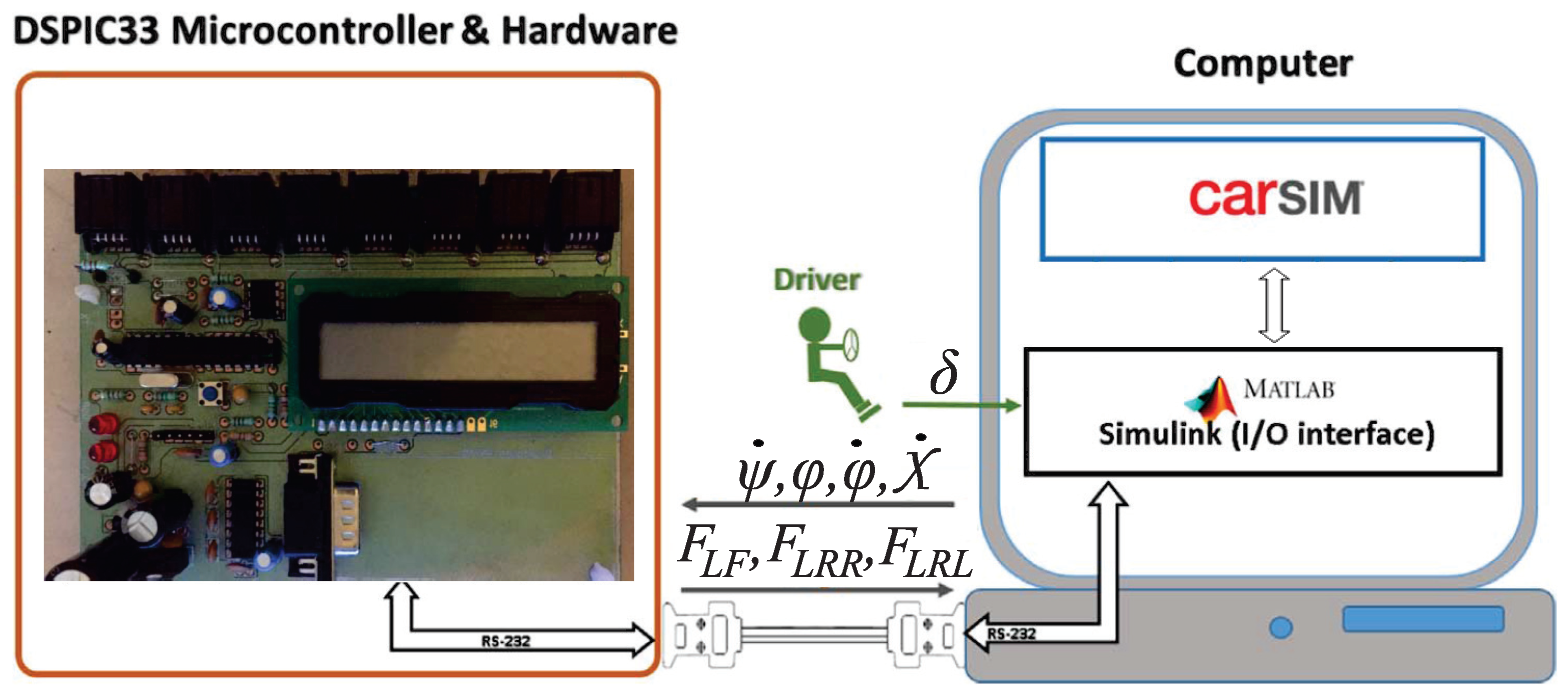
In this paper, new risk estimation indexes are developed to predict tripped and un-tripped rollovers as well as the skidding, considering the effects of the suspension system for TWVs. Such estimations can be easily calculated in a real scenario by chassis angular measures (obtained from an accelerometer) and are validated with the support of specialized software. Further, such estimations are used to design a new dynamic stability control (DSC) to mitigate tripped and un-tripped rollovers, as well as lateral and longitudinal skid risks, by differential braking/accelerating control actions. The design considers that potholes and speed bumps exist and can greatly increase the risk of rollover. Even more, the DSC is designed by means of robust control theory, to cope with the parametric uncertainty caused by changes in the mass, in the friction coefficient and in the height of the center of gravity, among other things; for this purpose, only nominal values have to be known. Implementation is ideal for electric TWVs, since they are able to generate correcting braking/accelerating differential torques and only require chassis angular information, obtained by an inertial measurement unit (IMU). Semi experimental tests with hardware-in-the-loop are presented to validate the effectiveness of the DSC.
Unlike previous works, in this article, tripped rollovers, the skid risk, the effects of the TWV suspension, road potholes and speed bumps, and semi-experimental tests with hardware-in-the-loop (HIL) are analyzed regardless of the traction/propulsion system.
The remainder of this paper comprises the mathematical modeling of the vehicle and lateral and longitudinal rollover risks, in
Section 2, along with the necessary validations. The analytic design of the DSC is presented in
Section 3.
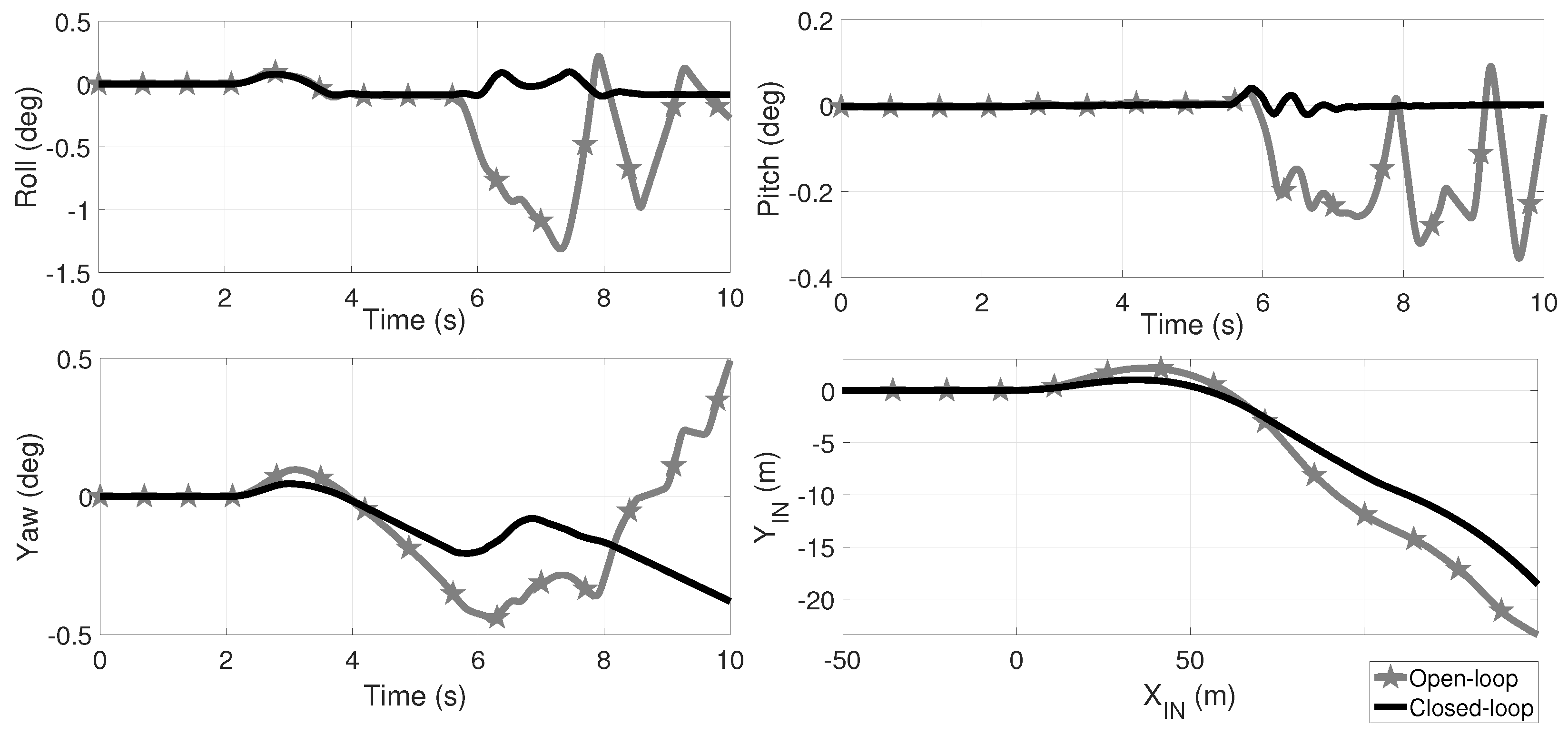
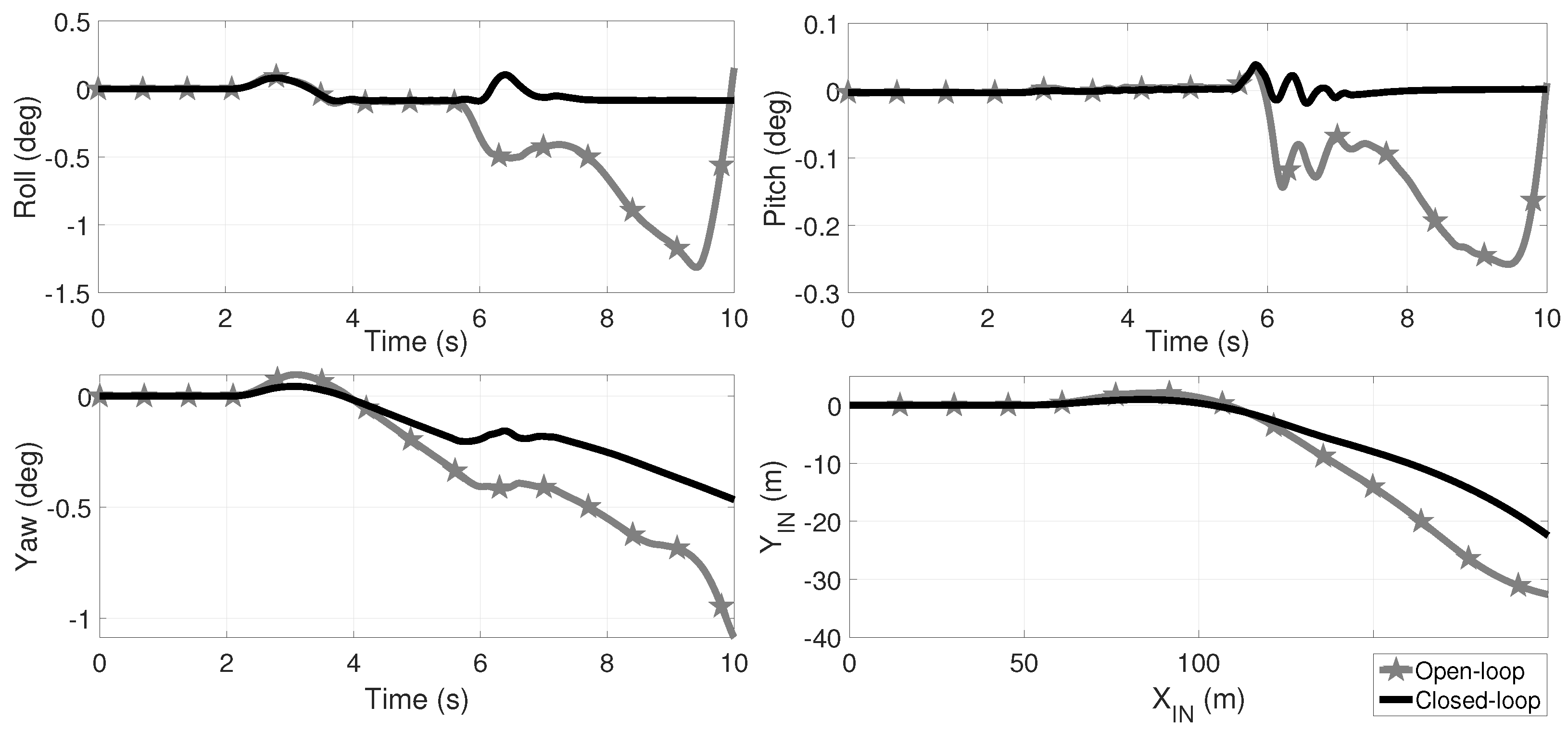
Section 4 is dedicated to showing the performance evaluation of the DSC, and the final section is dedicated to providing some conclusions and future work.
2. Modeling
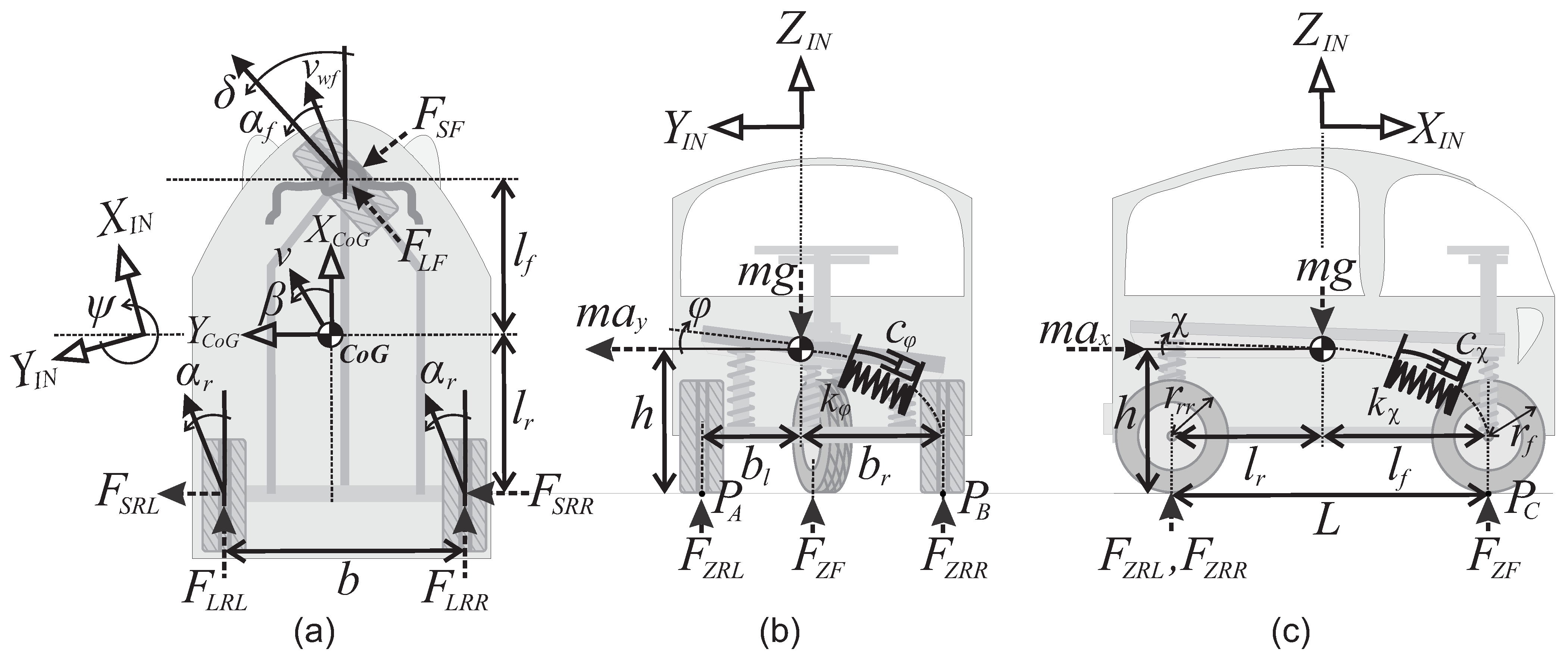
In this section, a rotational model of the TWV is presented; this model is obtained through the idealizations of
Figure 1. The main considerations/simplifications for this modeling are:
- (i)
Only small steering angles should be demanded, for high-speed driving (16 m/s and above).
- (ii)
Pitch and roll dynamics are decoupled.
- (iii)
For roll dynamics, the suspension can be simplified by a single rotational spring-damper system (with
and
coefficients respectively), for the torque-balance about the
-axis as shown in
Figure 1b.
- (iv)
For pitch dynamics, the suspension can be simplified by a single rotational spring-damper system (with
and
coefficients respectively) for the torque-balance about the
-axis as shown in
Figure 1c.
Such simplifications are opportune since it is not the objective of this investigation to obtain an exact model; rather, is to obtain a conservative estimate of the rollover and skid risks in order to calculate the control actions that mitigate such risks. The robust control theory used here allows facing uncertainty in the modeling and in the parameters (with limits). In
Table 1 and
Table 2 are described the associated nomenclature and parameters, respectively, along with a brief description, and nominal values where applicable.
2.1. Vehicle Model
From
Figure 1a and Consideration (i), longitudinal and lateral accelerations acting on the
(
reference frame) can be represented as:
Note that the gravitational, roll and wind exogenous forces are omitted; they are considered within the parametric variation ranges in the following sections. Longitudinal forces are considered the control-inputs and can be related to the braking/accelerating torque as:
Mechanical and regenerative braking are considered a single force for each wheel. Lateral forces can be conservatively approximated for small steering angles by a linear relationship with the tire sideslip angle ([
30] (p. 21), [
12,
31]). The tire side slip angles can be obtained from speed-balances over an inertial coordinate system
,
,
to obtain:
Note that these are conservative estimates of the lateral forces, since the real relationship is in fact sigmoidal [
30] (p. 157); a robust control approach allows for the design of a controller, despite variations on these formulations, in a posterior section. On the other hand, time-derivatives of the
displacement over the inertial coordinate system (
), transformation to the
coordinate system (
), and replacing Equations (
1) and (
5), allow us to obtain (see [
32] (p. 337) for a detailed similar procedure):
In order to represent the roll and pitch dynamics, torque-balances about
are performed (see
Figure 1b,c):
Substituting Equations (
1) and (
5) and considering
as a time varying parameter with some nominal value, using
(
denotes the transpose matrix or vector) and
, the full TWV nominal model can be written as:
where
2.2. Modeling the Rollover Risk for Roll Angle
The lateral load transfer ratio also is known as rollover index (
), and is a dynamic indicator of lateral rollover risk [
33,
34]:
The above calculation represents a normalized difference on the vertical forces about the lateral dynamics of the TWV; absolute values near one indicate a high risk of rollover since the vertical force on the tire-ground contact point (hereinafter only vertical force will be mentioned to refer to it) of a rear-wheel is almost null and the wheel can easily lose its tire-ground contact. An value indicates a left turn and imminent rollover risk to the right, and indicates a right turn and imminent rollover risk to the left.
An RI estimation that considers the suspension system can be obtained by substitution of the above vertical forces. In order to estimate such vertical forces on each tire-ground contact point, torque balances on
,
, and
are performed (see
Figure 1):
Substituting in Equation (
11):
Note that the formulation has been left in terms of the lateral and longitudinal accelerations because its real-time calculation is relatively simple through the use of an inertial measurement unit and knowledge of the associated parameters. Also note that this formulation does not depend on the road bank, wind speed nor direction, and can reproduce the effect of speed bumps or potholes on the dynamics of the vehicle.
2.3. Modeling the Rollover Risk in Pitch Direction
The longitudinal rollover risk, in this paper, occurs when the front tire or both rear tires lose contact with the ground; this type of maneuver is colloquially known as a wheelie or stoppie. To the author’s knowledge, there is no estimate of the risk of longitudinal rollover like the for the risk of lateral rollover.
Under premises similar to those proposed for the
, it can be inferred that a new longitudinal rollover risk can be calculated as the normalized difference of the front vertical force on the wheel, minus the vertical forces on the rear wheels:
Absolute
values near one indicate a high risk of longitudinal rollover since the vertical force on the front wheel, or both rear wheels is/are almost null, and easily can lose its/their tire-ground contact. For instance, an
value indicates a prominent rear load and imminent backwards rollover risk. Substituting (
12)–(
14) in (
16):
Again, this formulation does not depend on the road bank, wind speed or direction, and can reproduce the effect of speed bumps or potholes on the dynamics of the vehicle.
2.4. Modeling the Skid Risk
From the well-known friction ellipse idealization, tires’ adhesion occurs when:
If the above inequality does not hold, one or more tires lose adhesion and the vehicle can skid. By triangle’ inequality and substitution of Equations (
5) and (
8), a new skid index is proposed:
values near one indicate a high risk of vehicle sliding, and hence, a high risk of collision. Note that the skid index can be also easily calculated in a real application by measures of the chassis angles. Also, this formulation does not depend on the road bank, wind speed or direction. Although there is a dependence on the friction coefficient, in later sections a robust controller is designed in the event of changes in this and other parameters.
2.5. Integrating the Risks in the Vehicle Model
For completeness purposes, the formulations of risk indexes can be expressed in terms of the state variables of the dynamic system (
10). This is achieved by substituting the longitudinal and lateral accelerations:
These equations are provided to the reader as a reference for future designs.
2.6. Validation
In this research, a trial version CarSim (Mechanical Simulation Corporation) and Simulink (MATLAB) software are used. The validation of the risk indexes (
,
and
) will be carried out with the parameters of
Table 1 and
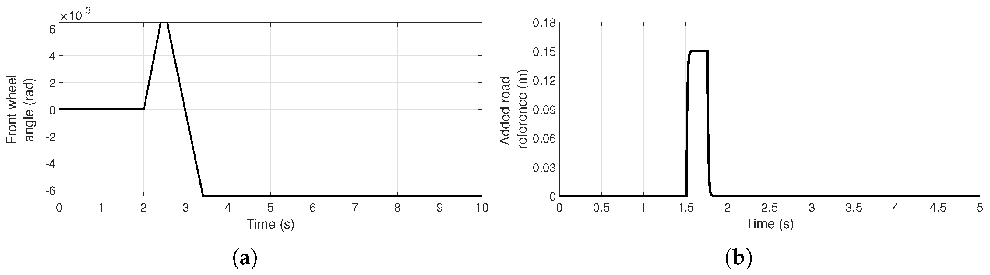
Table 2; in some cases, they are modified to induce some risk. Some parameters cannot be obtained directly from CarSim, such as the stiffness-coefficients of tires and suspension; these parameters are obtained from linearization of the curves provided by CarSim for aggressive driving (without a wheel lift or a skid). For the following tests, the fish-hook maneuver illustrated in
Figure 2a is used.
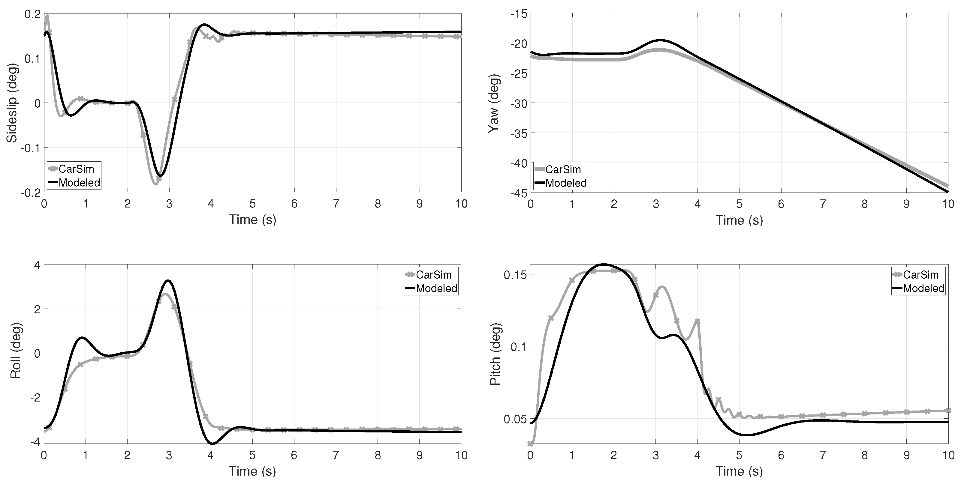
Figure 3 shows comparatives of the state variables (angles); such variables are calculated employing the model and compared with against those provided by CarSim. The vehicle speed is initialized to 22 m/s and left open throttle (no braking/accelerating torque in the wheels, only rolling resistance is stopping the TWV). The dynamic behavior of the model presents in average minimal error; this validation allows to show that the model is adequate for a control design in such operating point. Parameters as the stiffness-coefficients of the tires and suspension are tuned for such maneuver and are shown in
Table 2. For the pitch angle validation, a 100 N braking force in the front wheel is entered, otherwise, the pitch angle is almost constant along with the maneuver.
The risk indexes are validated by comparison with those obtained from CarSim by direct calculation from its definitions (Equations (
11), (
16) and (
18)); this software provides the longitudinal, lateral and vertical forces on the wheels. Since CarSim does not provide the angular accelerations for roll and pitch, these are calculated in Simulink; regardless of the above, the calculation of the risk indexes can be done in a real application by using an IMU and proper signal conditioning.
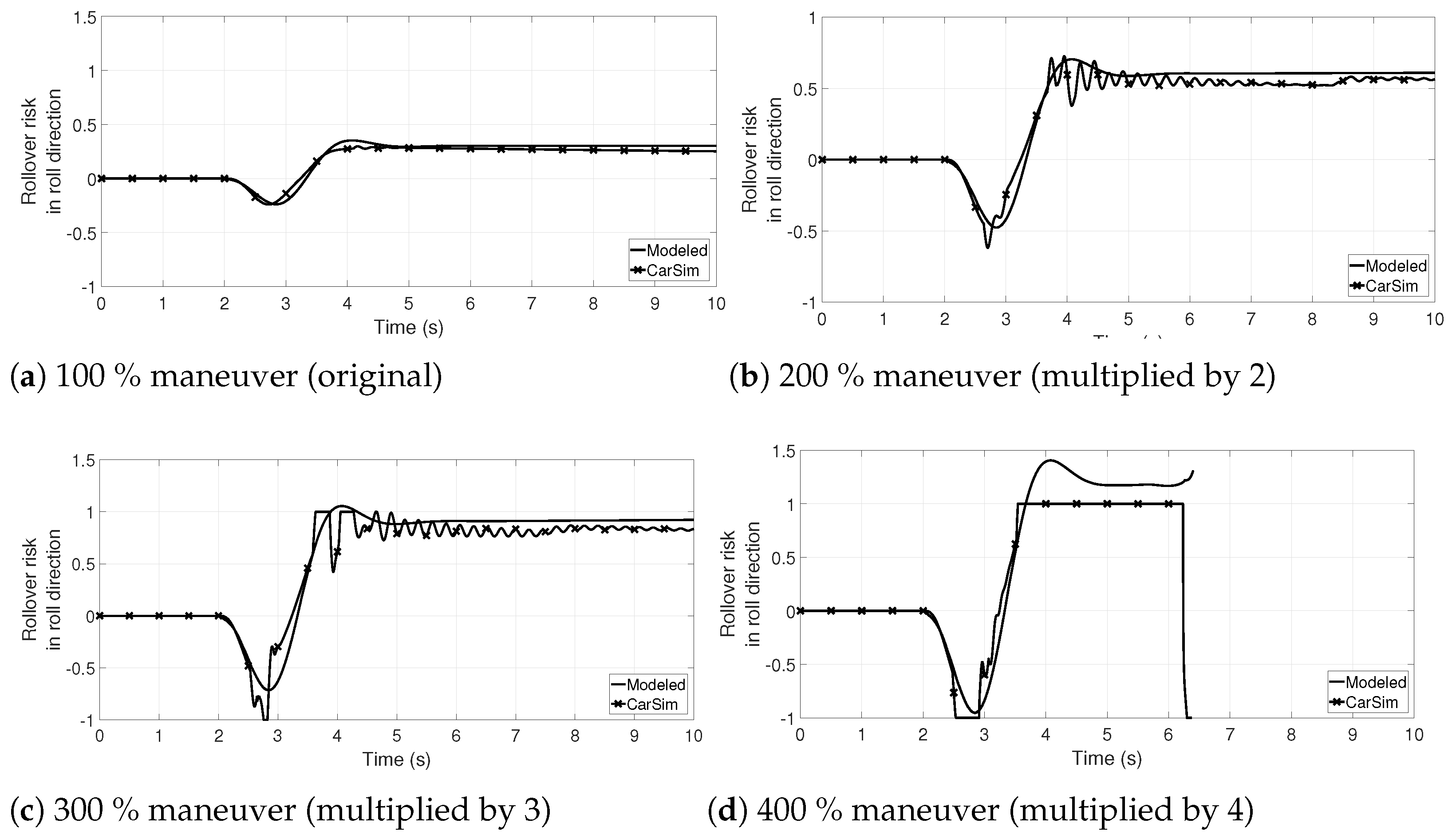
In order to validate the risk of rollover in the direction of the roll angle, the fish-hook maneuver of
Figure 2a is used but increased in steps of 100 up to
. In
Figure 4 comparatives of the
for such maneuvers are shown. Again, although the model cannot reproduce rapid oscillations (caused by the soft suspension of the TWV), it is sufficient to predict if there is a risk of rollover in the direction of
. With the maneuver increased by
, there is a loss of vertical force in a rear wheel, and the risk index is one or more (absolute value) in such intervals. With the maneuver increased by
, there is a lift of the right rear wheel and the vehicle ends up completely overturning.
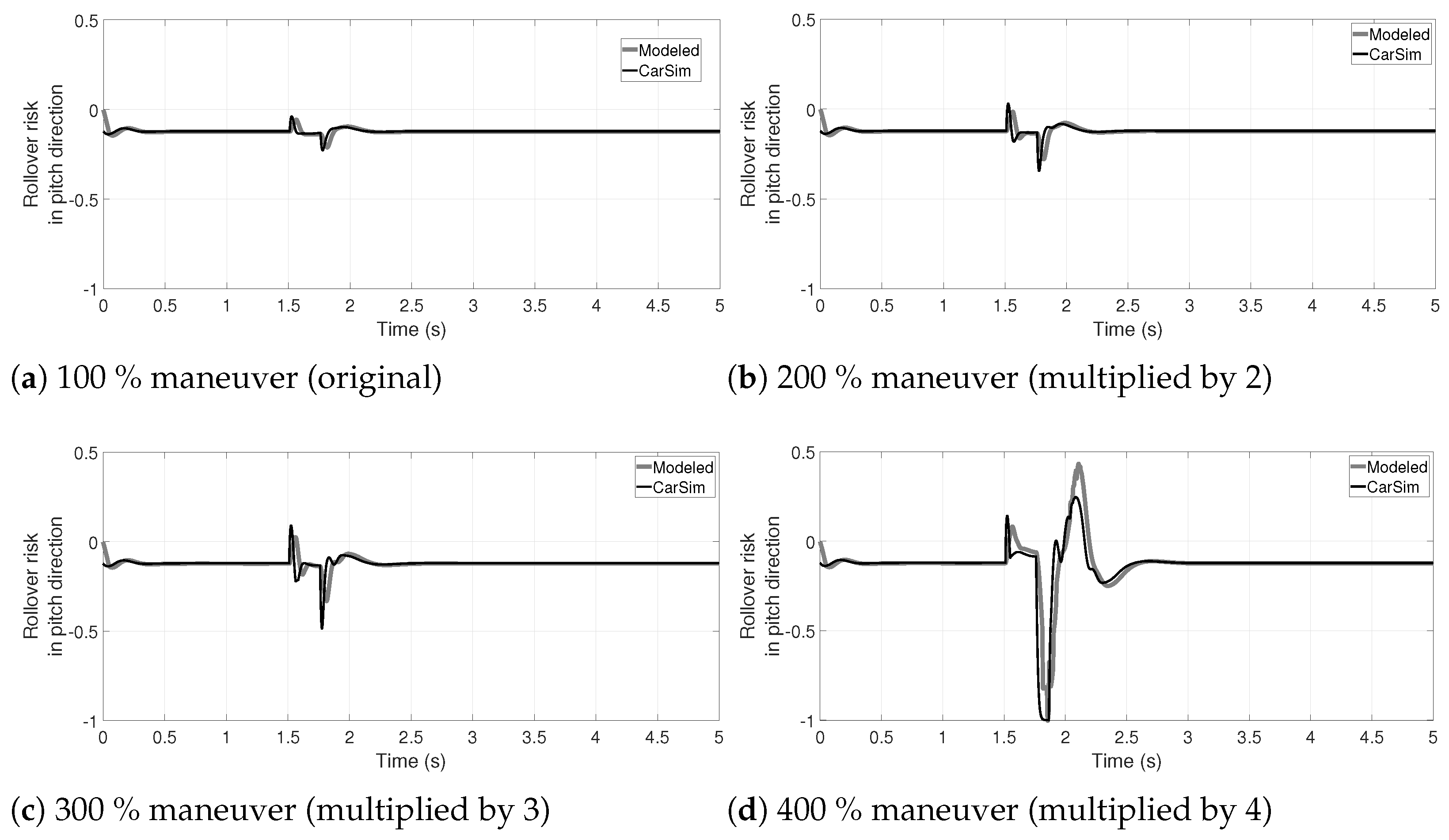
The rollover index risk in the direction of the pitch angle is validated by the introduction (adding) of a vertical road reference pulse (simulating a speed bump); if it is of sufficient height, this lifts the front wheel. The pulse of
Figure 2b is used, with increments of
up to
.
Figure 5 shows comparatives of the modeled rollover risk in the pitch direction against the calculation of Equation (
16). With the pulse augmented by
, the front wheel tipping is obvious at second
.
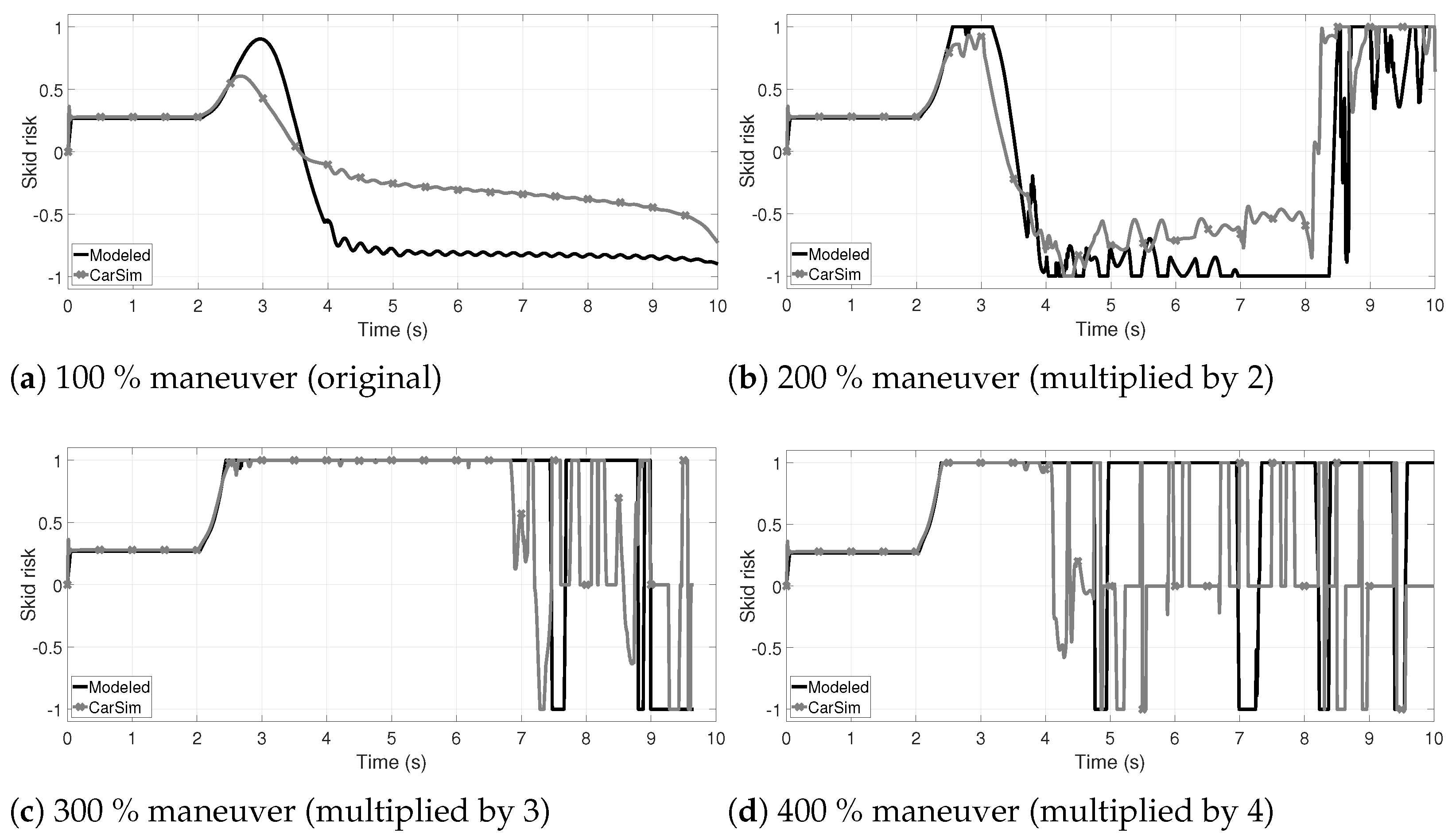
In order to validate the skid risk index, the friction coefficient is set to
and a 150 N rear accelerating force on each rear wheel is applied. With such a parameter combination is extremely easy to induce a tripped rollover; that is, the vehicle skids until it rollovers. The fish-hook maneuver of
Figure 2a is used again, augmented by steps as in the previous cases. In
Figure 6 the skid index comparisons are shown. For the
maneuver exclusively, the TWV can follow the fish-hook maneuver without a tripped rollover neither a skid. In this case, the modeled
shows a more conservative estimate of the risk; also, once a wheel of the TWV has been lifted, the estimation is erratic. This is because a mitigation system must interact to avoid the
reaching absolute values near one.
It is worth mentioning that the combination of a low coefficient of friction with speed bumps, potholes and/or other vertical exogenous forces during a maneuver, such as the fish-hook one (a combination of high risks’ levels, shown in later sections), considerably increases the risk of an accident.
It is worth mentioning that all taken considerations for the modeling result in a conservative estimation of the risks, as shown in the previous figures. Hence, although the presented models are not suitable for an accurate description of the TWV dynamics over all possible conditions and scenarios, it is enough and tractable for the design of a DSC following a conservative objective of mitigating the risks.
3. Robust Mitigation System Design
From equations for risk indexes (
11), (
16) and (
18), a state-feedback of the state-variables
,
,
, and
is suitable to diminish the risk indexes. The pitch angle (
) must not be included since it is not desirable to correct the longitudinal unbalance of the
(rarely the
is longitudinally centered in a real a TWV). Even more, such state variables are easily obtained by an IMU and the calculation of the risk indexes is not necessary for feedback (only during the design).
In order to generate a counter torque in the direction of the yaw angle (contrary to the curve), it is proposed that one rear wheel brake and the other accelerate, with a force magnitude as close to equal as possible. Also, in this way, the risk of skidding will not be increased because the terms
,
are almost canceled out in Equation (
19). Also, for a rollover risk in the pitch direction, all-wheel braking/accelerating with an equitable distribution on front/rear wheels is proposed, to contribute to the differential braking/accelerating control law.
The proposed control law (
,
and
) for the system of Equation (
10) is then:
In order to find suitable values for the control gains matrix K under arbitrary but bounded parameter-varying, first the closed-loop system is coordinate-transformed (the stability property of a system is preserved for an operating point shifting). Later, a polytopic representation is obtained, whose vertexes are calculated with the bounds for the K entries and a global parameter variation conservatively proposed as a scaling factor; LMI software allows one to numerically determine the bounds of the K entries for a common Lyapunov function. Subsequently, the best K entries are obtained by an optimization algorithm.
The closed-loop system turns on:
where
Consider the linear variable change
with
(see [
36] (p. 112)); then the dynamic system (
22) turns in:
In order to establish robust stability for the closed-loop system (
23) against model and parameter uncertainty, a polytopic representation is defined and a common Lyapunov function is foreseen to ensure stability despite arbitrary-rate varying-parameters. Consider a bounded parameter variation as follows:
where
is a real number. For instance,
represents a
global variation of parameters. Note that this is a more conservative definition of uncertainty than those defined by independently varying entries of
A; the vertexes can be obtained for a particular set of uncertain parameters while the following analysis is still valid. Hence, two vertexes are obtained,
and
, where
(a maximum steering angle) is used.
Under regular parameter values (generally
,
,
), the vertexes meets the Sylvester’s criterion for negative definite matrices if:
ensuring the stability of each vertex. However as [
37] (p. 2) confirms, is not enough to ensure the stability of each vertex, to ensure the global stability of the linear time-variant system (
24). Instead, a common Lyapunov function ensures the global stability under arbitrary (abrupt but bounded) parameter varying, and even under arbitrary switching between vertexes. To this end, upper bounds on
are established (they are numerically unknown yet), then
increasing the number of vertexes to
:
calculated with , , and named ,
calculated with , , and named ,
calculated with , , and named ,
calculated with , , and named ,
...
calculated with , , and named .
calculated with , , and named .
Therefore, the system (
24) turns into the polytopic system:
A common Lyapunov candidate function is
, such that one looks to find a positive definite matrix
P ([
38] (p. 9)) such that:
Therefore,
must be negative definite matrices. The determination of
P can be carried out numerically, for example, using the MATLAB library called YALMIP [
39]. Its existence depends on the parameters, and the
and
values. In the following, an algorithm (Algorithm 1) is presented to numerically find appropriate values for
P,
,
, and
.
| Algorithm 1 An algorithm is presented to numerically find appropriate values for P, , , and . |
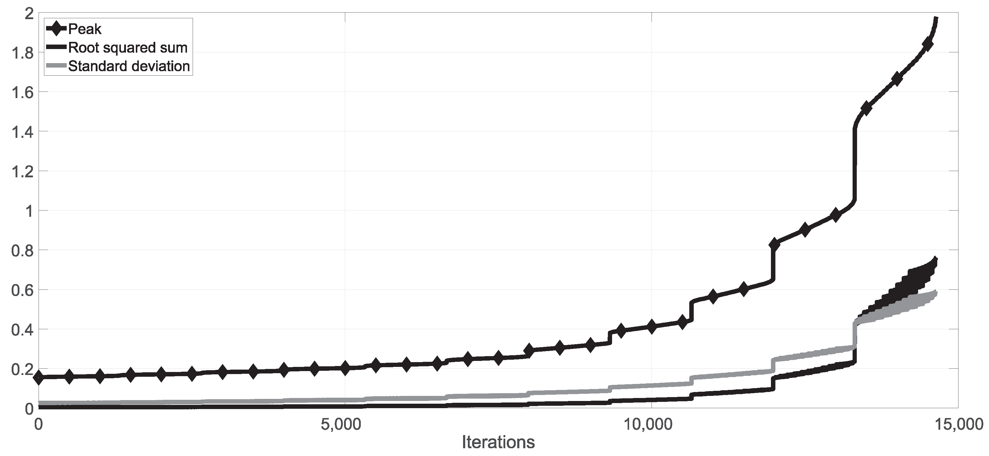
Initialize and , . Try to solve the LMI, . If P cannot be found, verify the used parameters. Increase and decrease by small steps and try to solve the LMI, . Repeat the Step 3 if P is found. If P cannot be found anymore, fix the smaller and largest values for which the LMI has a solution. If go to Step 9. Decrease by a small step and try to solve the LMI, . If P cannot be found, set . If go to Step 12. Decrease by a small step and try to solve the LMI, . If P cannot be found, set . If go to Step 15. Decrease by a small step and try to solve the LMI, . If P cannot be found, set . If go to Step 18. Decrease by a small step and try to solve the LMI, . If P cannot be found, set . If ∧∧, then go to Step 20. Go to Step 6. Solve the following optimization problem, to find
where T is a time horizon. End
|
In Algorithm 1, one looks to find the first bounds for the parametric variation. Then, bounds for the controller gains are found, and finally, one looks for the combination of gains (within the bounds for stability) that the best results provide for minimizing the risks. In
Section 4, the resolution of the Algorithm 1 for the parameters of
Table 1 is exemplified. Also, note that exogenous perturbations can be added during Step 20 to emulate a driving with speed bumps for instance.
Resolution of the Algorithm 1, ensures the robust stability of the system for any parametric variation within the bounds, provides bounds for the controller gains and ensures the best performance (tuning) of the controller on minimizing the risk.
Although another criterion other than the squared maximum risk could have been selected on Step 20, such as the mean square error or the standard deviation, this was chosen for its fast calculation; as well, the result is in practical terms the same. In
Section 4, the resolution of Algorithm 1 for the parameters of
Table 2 is exemplified; both criteria, the mean square error and standard-deviation, are included in such exemplification.


