Model for the Pattern-Dependent Wet Grip Prediction of Tires

Abstract

The most important task of the tire is to ensure driving safety by optimally transmitting the required longitudinal and lateral driving forces. Although great progress has been made in the past in the development of new materials and patterns, many questions remain unanswered in the field of elastomer friction on rough surfaces. This is particularly true when an additional intermediate medium is introduced into the contact, as for braking on wet roads in the form of water. To better understand this process, a model of a single-tread block on a rough road surface is developed. The influence of the fluid is represented by a physical meaningful friction law. The model is validated with results of tire wet-braking tests on an internal drum test rig. The model can map the interaction between tire tread, rough road surface and fluid film and the simulation results show a good agreement with the measurement results. Based on the investigation of individual tread blocks, a new approach to the description of the wet-braking behavior of passenger car tires was thus demonstrated, which can be extended to more complex tread geometries in the future.

1. Introduction

The main function of tires is to ensure safe driving by optimally transmitting the required braking and steering forces. When braking on wet roads, many parameters play a role. These include the properties of the tire rubber, the tread geometry of the tire, the nature of the road surface as well as the driving speed, internal tire pressure and water height. Although great progress has been made in the past in the development of new materials and patterns, many questions remain unanswered in the field of elastomer friction on rough surfaces. This is particularly true if an additional intermediate medium is introduced into the contact, such as for braking on wet roads in the form of water. This application will be examined in detail here to gain a deeper understanding of the processes in the tire contact area during wet braking by means of tire simulations and tire measurements.

The main mechanisms of force transmission between rubber and road surface are hysteresis and adhesion. According to Persson adhesion only contributes significantly to the total friction on very clean and dry surfaces [1]. In addition to his own arguments, he also relies on a publication by Fuller and Tabor [2]. However, he is of the opinion that the lack of adhesion as the only explanation is not sufficient to explain the different coefficients of friction on wet and dry surfaces. In [3] he attributes the effect to a smoothing of the power spectrum by enclosed water pools and thus to a reduction of hysteresis friction. A different opinion is expressed by Schramm. He concludes from the comparison of measurements with water and oil as an intermediate medium that if water is used as an intermediate medium, the adhesive friction has a considerable share ([4], [p. 65]). However, there is broad agreement that the most important mechanism is the remaining hysteresis friction of the rubber ([5], [p. 36]), [3,6,7,8,9,10]. In addition, there is a contribution of viscous friction due to the shear of the fluid film. However, this is neglected in most cases. Do et al. investigate in [11] the influence of micro-roughness on the coefficient of friction at water heights below one millimeter. Although the coefficient of friction of pavements without microtexture decreases as soon as the road surface is wet, this decrease occurs at higher water heights in the case of greater micro-roughness.

In [12], Kane and Cerezo present a model to describe hysteresis friction on dry surfaces. The visco-elastic behavior of the rubber is modeled by a Kelvin-Voigt element and the frictional force results from the asymmetry of the pressure distribution on the uneven road surface. This model is extended in [13] by the intermediate medium water. For this purpose the influence of the fluid is modeled using a so-called ’pseudo’-hydrodynamic plain bearing model. Using the Reynolds equation, the hydrodynamic buoyancy force is determined and deducted from the normal force when calculating the friction forces. The model predicts a strong decrease of the coefficient of friction at low macro-roughness and high speeds, whereas the coefficient of friction decreases only very moderately at high macro-roughness. Similar measurement results regarding the influence of micro-roughness at low water levels can be found in [14].

In [15] Persson investigates the fluid dynamics in the contact area of an elastic solid with a rough surface. The theory of the effective medium according to Bruggeman [16] is used to describe the influence of the road surface roughness on the fluid flow. The direct contact between elastic solid and rough surface is described by Perssons contact theory [17,18]. Inertial effects of the fluid are neglected due to the low fluid film height. Furthermore, the theory takes into account the anisotropy of the rough surface on different length scales.

Golden presents in [19] a physical model based on the contact model of Greenwood and Williamson [20] and the time dependence of the water film height with the theory of Moore [21]. Basic rubber properties, the road surface texture and the geometry of the contact surface are considered. However, the influence of the pattern is only considered in a simplified way via the existing negative pattern void.

Wagner et al. map the hysteresis friction using a multi-scale model [22]. The adhesion component is neglected here for the case of a wet road surface. The fluid only plays a role by preventing the adhesion component, but it has no influence on the hysteresis component. In a later publication the adhesion component will be considered, but the investigations only concern relatively low sliding velocities up to 10 $\mathrm{mm}$ $\mathrm{s}$⁻¹ [23] and are therefore not meaningful for braking on wet roads.

Contact between the rubber and the road surface on many length scales is necessary for the transmission of braking forces through hysteresis friction. For this purpose, the water film in contact must be squeezed out. In contrast to aquaplaning, the inertia of the water plays only a minor role when the road surface is only damp or wet due to a low water level. How quickly the water can be displaced from the contact area therefore depends primarily on the viscosity of the fluid, the local surface pressure, the relative speed between rubber and road surface and the texture of the road surface. The local contact conditions depend on the tread pattern and the properties of the rubber. Longitudinal and lateral grooves, as well as the distribution of the negative tread, no longer play such a decisive role here, since the drainage of the entire tire footprint is not critical due to the low water height.

To better understand the processes in contact, the commercial FEM program ABAQUS is used to build a model of a single-tread block on a rough road surface. Three different tread geometries are modeled. Pattern BB (big blocks), pattern BBs (big blocks with sipes) and pattern SB (small blocks). The three patterns used are shown in Figure 1. The block dimensions are described in detail in Appendix A. These rather simple three patterns were selected to reduce the complexity of the model and to allow conclusions to be drawn about individual effects when discussing the model results. The influence of the viscous fluid film between the rubber and the road surface is represented by a phenomenological friction law.

The aim of this model is to calculate the forces acting on a single-tread block when passing through the tire contact patch on a wet road.

The simulation results are then validated with measurements that were performed with test tires on the KIT (Karlsruhe Institute of Technology) inner drum test rig on a real asphalt road. The pattern of the test tires is composed of individual tread blocks that correspond to the tread blocks shown in the model. Therefore, the test results can be used to validate the model, although only a single-tread block is modeled.

2. Testing

The internal drum test bench of the Institute of Vehicle System Technology, which is schematically shown in Figure 2, offers the possibility of carrying out braking tests with individual car tires under controlled ambient conditions. It consists of a steel drum with an inner diameter of $3.8$ $\mathrm{m}$, which is driven by an electric motor. The drum is equipped with asphalt-loaded steel cassettes. The tire is driven by a hydraulic motor. Wheel load, camber and slip angle are also adjusted by a hydraulic system. The resulting forces and torques which are acting on the tire are measured with a 6-component measuring hub and recorded with a frequency of 100 $\mathrm{Hz}$. The internal tire pressure is controlled during the entire measurement and thus kept constant. For wet measurements, water is applied to the road surface behind the tire in the direction of travel. The water is then distributed evenly on the road surface under the influence of the centrifugal forces within three quarters of a revolution of the drum. The water level is measured by a capacitive sensor shortly in front of the tire and the water inflow is adjusted by an automatic control. In this way, a water level averaged over the circumference of the drum is set, but locally the water level can vary on the different segments of the roadway. Since capacitive measurement is used, 1 $\mathrm{m}$$\mathrm{m}$ water height describes the water quantity of 1 $\mathrm{L}$ ${\mathrm{m}}^{-2}$. Depending on the structure of the roadway, a water level of 1 $\mathrm{m}$$\mathrm{m}$ does not yet result in a closed water film. A detailed description of the test stand can be found in [24,25].

During the measurement, the drum rotates at a constant speed, whereby the path speed of the drum corresponds to the travel speed to be investigated. During braking, the wheel is subjected to an increasing torque by the hydraulic motor. The $\mu$-slip curves measured here therefore describe the braking forces occurring at a constant track speed of the drum.

The raw data recorded with 100 $\mathrm{Hz}$ is first corrected according to Augustin and Unrau [26] for the influence of the drum curvature and then filtered. Then the coefficient of friction $\mu$ as the quotient of longitudinal force and wheel load is plotted over the slip and the Magic Formula according to Pacejka is parameterized for each individual measurement [27]. To reduce the sensitivity to outliers and vibrations in the measured raw data, the maximum coefficient of friction ${\mu }_{max}$ is calculated from the parameters of the Magic Formula.

To further reduce the influence of outliers and measurement inaccuracies, several measurement repetitions are performed for each parameter combination and then the mean value is calculated from the results. Since the skid resistance of the road surface can change slightly during the measuring period, reference measurements were carried out several times a day. These measurements were used to correct the influence of changing skid resistance.

3. Model

As shown in Figure 3, a defined normal force $F_z\left(t\right)$ is applied to the tread block and it is moved over the road surface in positive x direction with a given slip speed $v_s$. The normal force represents the part of the wheel load to be carried by the tread block. The influence of the viscous intermediate medium water is represented by a phenomenological friction law which will be described later. In the contact area, the shear and normal stress distributions $\tau (x,y,t)$ and $\sigma (x,y,t)$ result. If these are integrated, the free body diagram of the tread block with the reaction force $F_N\left(t\right)$ and the resulting braking force $F_x\left(t\right)$ on the right-hand side of the Figure 3 is obtained. It is assumed that the water inside the valleys of the macro-roughness, if there is any, does not contribute to the load support of the track, because the water film heights considered in this model are too small to cause significant fluid inertia effects. From this the global coefficient of friction

$$\begin{array}{cc}\hfill {\mu }_G\left(t\right)& =\frac{F_x\left(t\right)}{F_N\left(t\right)}\hfill \end{array}$$

(1)

is calculated. Due to the inertia of the block, $F_z\left(t\right)\ne F_N\left(t\right)$ is generally valid.

3.1. Phenomenological Friction Law

In case of lower water heights or a road surface that is only wetted, the viscosity of the water is of decisive importance. On the largest length scale there seems to be contact between rubber and the individual roughness peaks of the road surface. However, if the contact area is enlarged, it will be noticed that a viscous residual water film remains in the contact area. This initially prevents hysteresis friction on smaller length scales. The contact pressure of the rubber squeezes out the viscous residual water film more and more, thus enabling contact even on smaller length scales and thus the transmission of frictional forces through hysteresis friction. How quickly the water film can be squeezed out depends primarily on the viscosity of the fluid, the surface pressure, the size and geometry of the local contact areas and the micro-roughness of the road surface. A calculation of the viscous flow taking into account all length scales relevant for hysteresis friction is practically impossible, therefore a phenomenological friction law is introduced at this point, which must be parameterized. The aim of the friction law is the calculation of the local friction coefficient for the contact between rubber and road surface depending on the local pressure distribution in the contact area and its history. To derive the friction law, a temporally constant local pressure distribution $\overline{p}(x,y)$ is assumed. Thus, the temporal course of the local friction coefficient is determined by

$$\begin{array}{cc}\hfill \mu (x,y,t)& ={\mu }_{\infty }-({\mu }_{\infty }-{\mu }_0)e^{-\lambda \overline{p}(x,y)t}\hfill \end{array}$$

(2)

and its temporal change by

$$\begin{array}{cc}\hfill \frac{d}{dt}\mu (x,y,t)& =\lambda \overline{p}(x,y)({\mu }_{\infty }-{\mu }_0)e^{-\lambda \overline{p}(x,y)t}.\hfill \end{array}$$

(3)

The limit friction value ${\mu }_{\infty }$ describes the maximum friction value that can be achieved if a sufficiently long time t is available to squeeze the fluid in contact. ${\mu }_{\infty }$ thus summarizes the influence of the pavement texture on the coefficient of friction, if the viscous fluid film is neglected. $\lambda$, on the other hand, describes the influence of the surface texture on the squeeze-out of the viscous fluid film. The initial coefficient of friction ${\mu }_0$ describes the coefficient of friction at the moment of first contact. In this case, the viscous water film is still closed, and forces are only transmitted via the viscosity of the fluid. The temporal course of the coefficient of friction is determined by the parameter $\lambda$. This indirectly reflects the viscosity of the fluid and the micro-roughness of the road surface. The lower the viscosity of the fluid and the higher the micro-roughness of the road surface, the faster the fluid is squeezed out and the faster the coefficient of friction increases. This corresponds to a large value of $\lambda$. If a sufficiently long time is allowed, the limit friction value ${\mu }_{\infty }$ is always reached, regardless of $\lambda$. The course of the friction value over time is shown in Figure 4. The exponential and limited course of the coefficient of friction is based on [28]. Lorent et al. establish there an exponential and restricted relation between time and contact pressure, or between time and the distance for squeezing a fluid between a smooth elastic and a rough rigid surface. It is, therefore, assumed in the following that the coefficient of friction develops similarly to the contact pressure and the distance between the surfaces mentioned in [28].

In general, there is no constant pressure distribution over time. Therefore, the friction coefficient map

$$\begin{array}{cc}\hfill {\mu }_k(p_k,\tau )& ={\mu }_{\infty }-({\mu }_{\infty }-{\mu }_0)e^{-\lambda p_k\tau }\hfill \end{array}$$

(4)

is defined. The total differential of the friction coefficient map is

$$\begin{array}{cc}\hfill \frac{d}{dt}{\mu }_k(p_k,\tau )& =\frac{\partial }{\partial \tau }{\mu }_k(p_k,\tau )·\frac{d\tau }{dt}+\frac{\partial }{\partial p_k}{\mu }_k(p_k,\tau )·\stackrel{=0}{\overbrace{\frac{d{p}_k}{dt}}}.\hfill \end{array}$$

(5)

The temporal change of the surface pressure $d{p}_k·d{t}^{-1}$ is neglected here, since the absolute value of the surface pressure has a much larger influence on squeezing out the viscous residual water film than the temporal change of the surface pressure. This differential is now used to describe the change in the real coefficient of friction $\mu (x,y,t_i)$ at a point $x,y$ at a time $t_i$. First, the characteristic time $\tau (x,y,t_i)$ is calculated by transforming the Equation (4) to

$$\begin{array}{cc}\hfill \tau (x,y,t_i)& =-\frac{1}{\lambda \overline{p}(x,y,t_i)}ln\left(-\frac{\mu (x,y,t_i)-{\mu }_{\infty }}{{\mu }_{\infty }-{\mu }_0}\right)\hfill \end{array}$$

(6)

with $p_k=\overline{p}(x,y,t_i)$ and ${\mu }_k=\mu (x,y,t_i)$.

Figure 5 illustrates this calculation step. The current coefficient of friction $\mu (x,y,t_i)={\mu }_k$ and the current average surface pressure $\overline{p}(x,y,t_i)=p_k$ define a unique point in the characteristic diagram ${\mu }_k(p_k,\tau )$. According to Equation (6) this point can be assigned a characteristic time $\tau (x,y,t_i)$. This $\tau (x,y,t_i)$ represents the time which would have been necessary to reach the friction value $\mu (x,y,t_i)$ currently applied at the position $x,y$ under the assumption that the surface pressure $\overline{p}$ would have corresponded to the currently applied surface pressure $\overline{p}(x,y,t_i)$ the whole time. For this $\tau (x,y,t_i)$ the gradient

$$\begin{array}{cc}\hfill \frac{\partial }{\partial \tau }{\mu }_k(p_k,\tau ){|}_{\tau (x,y,t_i),p_k=\overline{p}(x,y,t_i)}& =\lambda \overline{p}(x,y,t_i)({\mu }_{\infty }-{\mu }_0)e^{-\lambda \overline{p}(x,y,t_i)\tau (x,y,t_i)}.\hfill \end{array}$$

(7)

can be read from the map. For this approach, the incremental change of the physical time $dt$ at the current time $t_i$ corresponds to the incremental change of the characteristic time $d\tau$, therefore the relation $d\tau ·d{t}^{-1}=1$ applies. The total differential of the friction value $\mu (x,y,t_i)$ is therefore

$$\begin{array}{cc}\hfill \frac{d}{dt}\mu (x,y,t){|}_{t_i}& =\frac{\partial }{\partial \tau }{\mu }_k(p_k,\tau ){|}_{\tau (x,y,t_i),p_k=\overline{p}(x,y,t_i)}.\hfill \end{array}$$

(8)

Equation (8) describes the temporal change of the coefficient of friction at a fixed position of the track. This corresponds to the assumption that the viscous residual water film determining the coefficient of friction is stationary on the track. However, due to the slip that occurs during braking, the rubber and the road surface shift relative to each other. If the viscous fluid film were to adhere completely to the rubber surface, the change of the coefficient of friction over time in the $x^{\prime },y^{\prime }$-coordinate system moving along with it could be described analogously to Equation (8) by

$$\begin{array}{cc}\hfill \frac{\partial }{\partial t}\mu (x^{\prime },y^{\prime },t){|}_{t_i}& =\frac{\partial }{\partial \tau }{\mu }_k(p_k,\tau ){|}_{\tau (x^{\prime },y^{\prime },t_i),p_k=\overline{p}(x^{\prime },y^{\prime },t_i)}.\hfill \end{array}$$

(9)

Figure 6 shows the $x,y$ inertial coordinate system and the relative coordinate system $x^{\prime },y^{\prime }$ shifted by the vector $\overrightarrow{r}$. $v_{s,x}$ describes the slip velocity of the rubber fixed point Q in x-direction. Due to the description in the relative coordinate system, which is also moved, the total differential at time $t_i$ results to

$$\begin{array}{cc}\hfill \frac{d}{dt}\mu (x^{\prime },y^{\prime },t){|}_{t_i}& =\stackrel{I}{\overbrace{\frac{\partial }{\partial \tau }{\mu }_k(p_k,\tau ){|}_{\tau (x^{\prime },y^{\prime },t_i),p_k=\overline{p}(x^{\prime },y^{\prime },t_i)}}}+\stackrel{II}{\overbrace{\frac{d{x}^{\prime }}{dt}}}\stackrel{III}{\overbrace{\frac{\partial }{\partial x^{\prime }}\mu (x^{\prime },y^{\prime },t){|}_{t_i}}}\hfill \end{array}$$

(10)

with

$$\begin{array}{c}\hfill {\left(\begin{array}{c}{x}^{\prime }\\ y^{\prime }\end{array}\right)}_{{\overrightarrow{e}}_{x^{\prime }},{\overrightarrow{e}}_{y^{\prime }}}={\left(\begin{array}{c}x\\ y\end{array}\right)}_{{\overrightarrow{e}}_x,{\overrightarrow{e}}_y}-\stackrel{=\overrightarrow{r}}{\overbrace{{\left(\begin{array}{c}{r}_1\\ r_2\end{array}\right)}_{{\overrightarrow{e}}_x,{\overrightarrow{e}}_y}}}.\end{array}$$

(11)

Part I describes the temporal change of the coefficient of friction at a moving point on the rubber surface according to the friction coefficient map introduced in Equation (4) and can be written analogous to Equation (7) as

$$\begin{array}{cc}\hfill \frac{\partial }{\partial \tau }{\mu }_k(p_k,\tau ){|}_{\tau \left(t_i\right),p_k=p(x^{\prime },y^{\prime },t_i)}& =\lambda \overline{p}(x^{\prime },y^{\prime },t_i)({\mu }_{\infty }-{\mu }_0)e^{-\lambda \overline{p}(x^{\prime },y^{\prime },t_i)\tau (x^{\prime },y^{\prime },t_i)}.\hfill \end{array}$$

(12)

Part II describes the time derivative of the relative coordinate

$$\begin{array}{cc}\hfill \frac{d{x}^{\prime }}{dt}& =\frac{d}{dt}(x-r_1)=-v_{s,x}\hfill \end{array}$$

(13)

and corresponds to the negative local slip velocity $v_{s,x}$ between rubber and road surface in x direction.

Part III is the partial derivation of the coefficient of friction in the moving $x^{\prime },y^{\prime }$ coordinate system. In general, this gradient cannot be represented in a closed form, but only approximated by the backward difference quotient

$$\begin{array}{cc}\hfill \frac{\partial \mu (x^{\prime },y^{\prime },t)}{\partial x^{\prime }}{|}_{t_i}& =\frac{\mu (x^{\prime },y^{\prime },t_i)-\mu (x^{\prime }{-}_{\Delta }{x}^{\prime },y^{\prime },t_i)}{\Delta x^{\prime }},\hfill \end{array}$$

(14)

with ${}_{\Delta }{x}^{\prime }=v_{s,x}·{}_{\Delta }t$ and ${}_{\Delta }t=t_{i+1}-t_i$. The backward difference quotient is used because the braking process gives a preferred direction for fluid transport in the direction of travel and thus in a positive x direction. It should be noted that unlike the time gradient, the spatial gradient is not calculated from the friction coefficient map ${\mu }_k(p_k,\tau )$, but from the local friction coefficient $\mu (x,y,t)$ actually present on the road surface. This is not known a priori, but the result of the numerical calculation with abaqus presented in Section 3.2.

For modeling the viscous effects of the fluid, it is assumed that the fluid adheres to both the rubber and the road surface, so the relative velocity between fluid and road, as well as between fluid and rubber, is zero. Since the relative velocity between rubber and road surface is much smaller in the normal (z-)direction than in the tangential (x-)direction, the linear velocity distribution in the fluid shown in Figure 7 on the left side is a good approximation.

This is now approximated by a binary velocity distribution, which has the same volume flow. This simplification is made because in the later FE simulation only the velocities and positions of the road and rubber surfaces are calculated. Since no fluid is present in the FE simulation, no velocity distribution can be calculated in this fluid, only the ones at the boundary surfaces of track and rubber. This results in the velocity distribution shown on the right. The viscous water film is thus divided equally between the road and rubber surface at a time t. Accordingly, for the change of the coefficient of friction according to Equations (8) and (10)

$$\begin{array}{c}\hfill \begin{array}{cc}\hfill \frac{d}{dt}\mu (x,y,t){|}_{t_i}& =\frac{1}{2}(\frac{\partial }{\partial \tau }{\mu }_k(p_k,\tau ){|}_{\tau (x,y,t_i),p_k=\overline{p}(x,y,t_i)}\hfill \\ \hfill & +\frac{\partial }{\partial \tau }{\mu }_k(p_k,\tau ){|}_{\tau (x^{\prime },y^{\prime },t_i),p_k=\overline{p}(x^{\prime },y^{\prime },t_i)}-v_{s,x}\frac{\partial }{\partial x^{\prime }}\mu (x^{\prime },y^{\prime },t){|}_{t_i})\hfill \end{array}\end{array}$$

(15)

results. If now the relative coordinate system is moved into the inertial coordinate system in the current time step, with $\overrightarrow{r}=\overrightarrow{0}$ we get

$$\begin{array}{cc}\hfill \frac{d}{dt}\mu (x,y,t){|}_{t_i}& =\frac{\partial }{\partial \tau }{\mu }_k(p_k,\tau ){|}_{\tau (x,y,t_i),p_k=\overline{p}(x,y,t_i)}-\frac{1}{2}{v}_{s,x}\frac{\partial }{\partial x}\mu (x,y,t){|}_{t_i}.\hfill \end{array}$$

(16)

The friction coefficient at time $t_{i+1}=t_i{+}_{\Delta }t$ is

$$\begin{array}{cc}\hfill \mu (x,y,t_{i+1})& =\mu (x,y,t_i){+}_{\Delta }t\frac{d}{dt}\mu (x,y,t){|}_{t_i}\hfill \end{array}$$

(17)

Inserting Equations (13) and (14) into Equation (16) lists

$$\begin{array}{cc}\hfill \mu (x,y,t_{i+1})& =\stackrel{I}{\overbrace{\frac{1}{2}\left(\underset{I.a}{\underbrace{\mu (x,y,t_i)}}+\underset{I.b}{\underbrace{\mu (x{-}_{\Delta }x,y,t_i)}}\right)}}+\stackrel{II}{\overbrace{{}_{\Delta }t\frac{\partial }{\partial \tau }{\mu }_k(p_k,\tau ){|}_{\tau \left(t_i\right),p_k=\overline{p}(x,y,t_i)}}}.\hfill \end{array}$$

(18)

Part I means that the coefficient of friction at one point P is calculated from the mean value of the coefficient of friction at exactly this point and the coefficient of friction at an adjacent point Q, which has exactly the distance ${}_{\Delta }x=v_{s,x}·{}_{\Delta }t$ from P. This maps the transport of the upper half of the fluid by adhering to the rubber surface moving with $v_{s,x}$, as shown in Figure 7 on the right. Part II represents the squeezing of the viscous residual water film by the contact pressure $\overline{p}(x,y,t_i)$ currently applied at the point P. The parameters $\lambda$, ${\mu }_0$ and ${\mu }_{\infty }$ must be determined by means of measurement data. A separate set of parameters must be defined for each material pairing of rubber and roadway, since these parameters describe the influence of the viscosity of the fluid, the micro-roughness of the roadway and the size and distribution of the local contact areas. For better understanding, pure longitudinal slip was assumed in the derivation of the friction law. In the later implementation of the friction law, however, slip in transverse direction is also taken into account.

3.2. Implementation in Abaqus

The model was implemented in Abaqus Explicit 2018. The most important settings are summarized in

Table 1. Overview of the most important settings in Abaqus.

Description	Setting
Element type block	C3D8R
Element type track	R3D3
Edge length block mesh	$0.5$$\mathrm{mm}$
Edge length track mesh	1 $\mathrm{mm}$
Material model block	Hyperelastic, mooney-rivlin Viscoelastic, mooney-rivlin
Contact formulation	KINEMATIC
Friction law	vfric
Solver	ABAQUS explicit
Large deformations	NLgeom = yes
Version	ABAQUS 2018

.

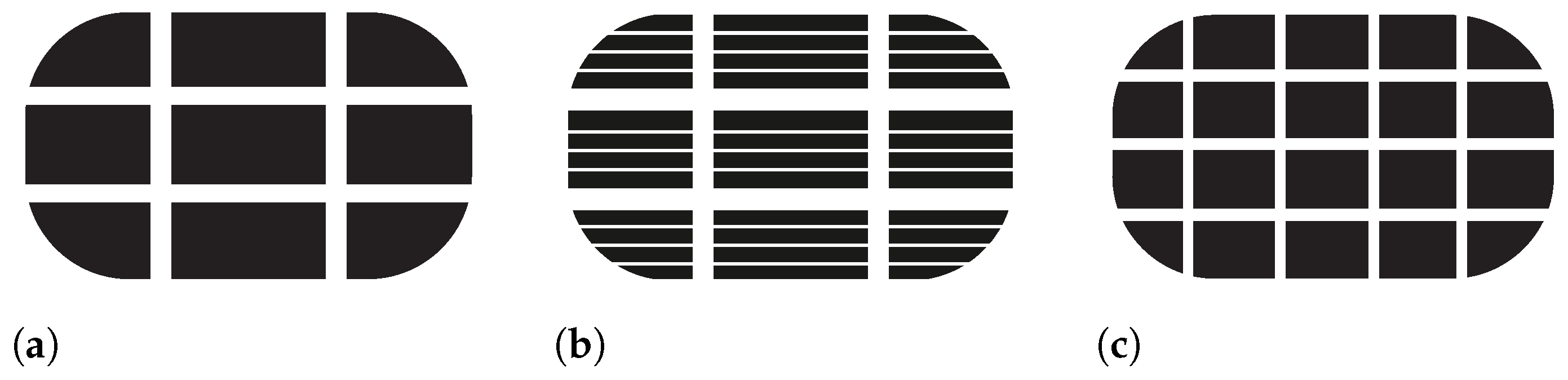
The roadway was modeled as a three-dimensional rigid body with R3D3 elements. The geometry of the roadway is based on a laser measurement of the asphalt surface. The measured raw data was first filtered and smoothed before the surface was meshed with an edge length of 1 $\mathrm{m}$$\mathrm{m}$. The pavement is fixed firmly in space. As pattern geometries the patterns BB (big block), BBs (big block with sipes) and SB (small block) shown in Figure 1 were modeled with C3D8R elements. Due to the underintegrated element types the ’hourglass control’ recommended by ABAQUS is used by default. The blocks have a height of $10.5$ $\mathrm{m}$$\mathrm{m}$, which corresponds to the tread depth of the test tires of $7.5$ $\mathrm{mm}$ plus the intermediate structure above the steel belt with a height of 3 $\mathrm{mm}$. The tread block was meshed with an edge length of $0.5$ $\mathrm{mm}$. The convergence of the model was investigated in [29]. 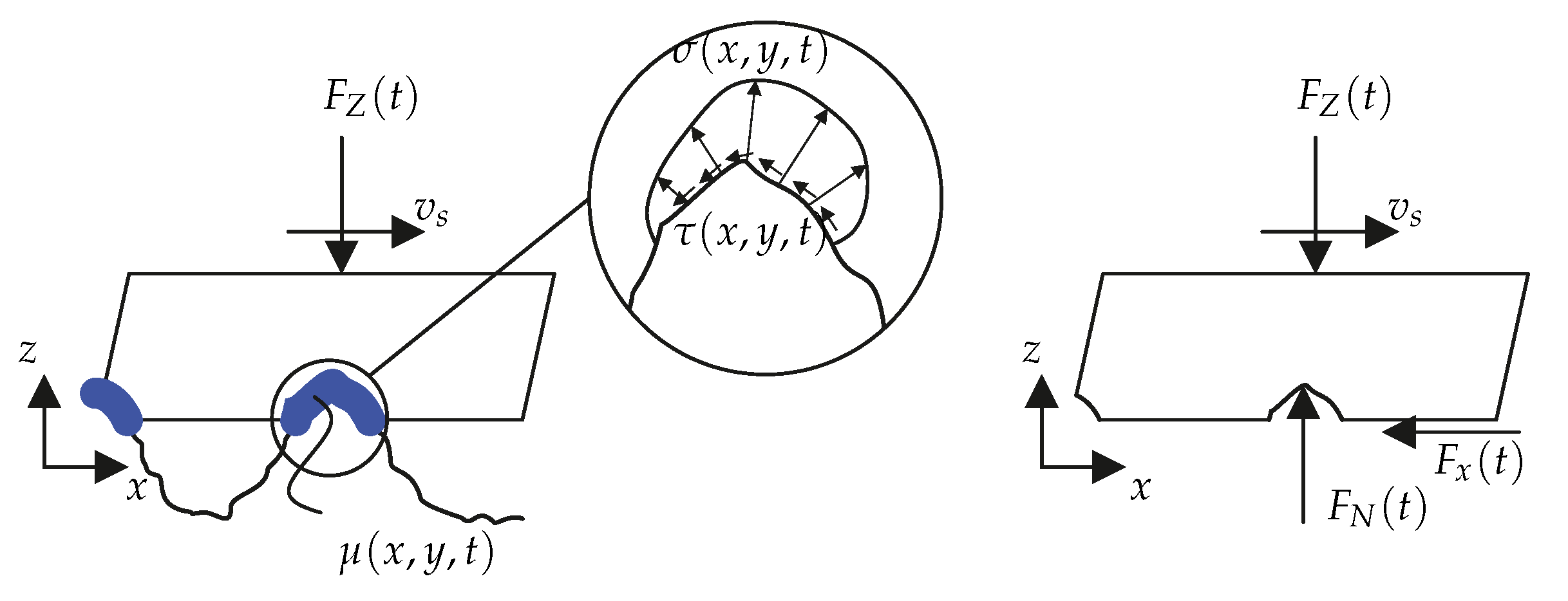Figure 8 shows the FE model consisting of roadway and block. The concentrated load $F_z\left(t\right)$ is converted to a surface load and acts on the surface $A_{Top}$. The constant slip velocity $v_S$ is specified for a node in the center of $A_{Top}$ as a start and boundary condition. All other nodes of the $A_{Top}$ surface are rigidly coupled to it, which corresponds to an infinitesimal flat, rigid and massless slab on $A_{Top}$. Both the contact between rubber and road surface and the self-contact of the rubber were implemented with the KINEMATIC formulation, because the use of the PENALTY formulation in combination with the subroutine vfric led to erroneous results. In this case, the specification of a constant coefficient of friction within the subroutine did not lead to the same result as the specification of a constant coefficient of friction without subroutine. The KINEMATIC formulation leads to the same result with a constant coefficient of friction with and without subroutine. This is again almost identical to the result of the PENALTY formulation without subroutine. Due to the computing time and the strongly non-linear behavior, caused by the large local deformations, an explicit integration method was used. The friction law presented in Section 3.1 was implemented in the subroutine vfric. A detailed description of this implementation can be found in Section 3.2.2.

The simulation time depends strongly on the pattern used and especially on the driving speed, since the contact time increases inversely proportional to the driving speed. Simulations with one core and an Intel(R) Xeon(R) Gold 6134 CPU ($3.2$ $\mathrm{G}$$\mathrm{Hz}$) result in the simulation times shown in

Table 2. Simulation time in Abaqus depending on pattern layout and driving speed when using an Intel(R) Xeon(R) Gold 6134 CPU ($3.2$ $\mathrm{GHz}$).

Pattern	Speed	Simulation Time
BB	50 $\mathrm{km}$ ${\mathrm{h}}^{-1}$	41 $\min$
BB	140 $\mathrm{km}$ ${\mathrm{h}}^{-1}$	17 $\min$
BBs	50 $\mathrm{km}$ ${\mathrm{h}}^{-1}$	119 $\min$
BBs	140 $\mathrm{km}$ ${\mathrm{h}}^{-1}$	41 $\min$
SB	50 $\mathrm{km}$ ${\mathrm{h}}^{-1}$	17 $\min$
SB	140 $\mathrm{km}$ ${\mathrm{h}}^{-1}$	7 $\min$

. The increased simulation effort due to the lamellas is clearly visible. On the one hand, this is due to the self-contact between the individual lamellae and on the other hand to the larger deformations in total.

Table 3. Smallest, largest and mean time increment during the simulation for the three investigated tire patterns.

Time Increment	BB	BBs	SB
Minimum	$3.303\times {10}^{-7}$$\mathrm{ms}$	$0.718\times {10}^{-7}$$\mathrm{ms}$	$3.296\times {10}^{-7}$$\mathrm{ms}$
Mean	$3.358\times {10}^{-7}$$\mathrm{ms}$	$1.492\times {10}^{-7}$$\mathrm{ms}$	$3.348\times {10}^{-7}$$\mathrm{ms}$
Maximum	$3.389\times {10}^{-7}$$\mathrm{ms}$	$2.183\times {10}^{-7}$$\mathrm{ms}$	$3.383\times {10}^{-7}$$\mathrm{ms}$

shows the minimum, maximum, and average time increments for the three different patterns. Although the increments for pattern BB and SB are relatively constant, there is a clear difference between the minimum and maximum values for pattern BBs. This is due to the large local deformation, which requires a significant reduction of the time step size.

3.2.1. Material Model

The rubber is modeled with hyperelastic and viscoelastic material properties. The hyperelastic behavior is defined by the Mooney-Rivlin model. The required parameters $c_{01}$, $c_{10}$, $D_1$ from [30] can be defined according to ([31], [p. 77]) via

$$\begin{array}{c}\hfill c_{10}=\frac{Ef}{4(1+v)},c_{01}=\frac{E(1-f)}{4(1+v)},D_1=\frac{6(1-2v)}{E}\end{array}$$

(19)

with the modulus of elasticity E, the transverse contraction number v and the nonlinearity factor f of the Blatz-Ko model [31,32]. The parameters

$$\begin{array}{c}\hfill E=2.8883 \mathrm{MPa},f=0.6398,v=0.495\end{array}$$

(20)

were used (Calculated with the Mooney-Rivlin-Parameters of material m1 from ([31], [Appendix C])).

The viscoelastic material behavior is approximated by Prony terms. By choosing the Prony parameters $E_k$ and ${\tau }_k$ accordingly, the course of experimentally determined curves of the storage and loss module as a function of frequency can be mapped. The equation for the complex module is thus [30,31]

$$\begin{array}{c}\hfill E^{*}\left(\omega \right)=E_{\infty }+\sum _{k=1}^n\frac{E_k{\tau }_k^2{\omega }^2}{1+{\tau }_k^2{\omega }^2}+i\sum _{k=1}^n\frac{E_k{\tau }_k\omega }{1+{\tau }_k^2{\omega }^2}.\end{array}$$

(21)

The following applies

$$\begin{array}{cc}\hfill E_{\infty }& =E(\omega \to 0)\mathrm{and}\hfill \end{array}$$

(22)

$$\begin{array}{cc}\hfill E_0& =E(\omega \to \infty )=E_{\infty }+\sum _{k=1}^n{E}_k\hfill \end{array}$$

(23)

for the static module $E_{\infty }$ and the instantaneous module $E_0$. Figure 9 shows the course of the storage modulus $E^{\prime }$ and the loss modulus $E^{″}$ as a function of the angular frequency $\omega$ for the rubber material used in this work.

3.2.2. Local Friction Law

The friction law described in Section 3.1 was implemented with the Abaqus subroutine vfric using the programming language Fortran 77 [33]. The roadway was defined in contact as master (surface) and the tread block as slave (surface). Based on Equation (18), the friction value ${\mu }_{s_j}\left(t_{i+1}\right)$ is calculated for each node $n_{s_j}$ of the slave surface at each time step $t_{i+1}$ (see Figure 8). The index j numbers all slave nodes in contact with the road surface. The local surface pressure ${\overline{p}}_j$ at the corresponding node is available from the simulation. The time increment ${}_{\Delta }t$ is determined by the step size of the solver. The parameters $\lambda$, ${\mu }_0$ and ${\mu }_{\infty }$ are passed to the program as constants before the simulation starts.

Table 4. Representation of all vectors used in the implementation in Abaqus. Line 1 contains the name of the vector, line 2 marks the entries of the corresponding vector. Line 3 summarizes the size of the vector and line 4 indicates the run index, which is used to increment the entries of the vectors.

Name	$\overrightarrow{{\mathit{\mu }}_{\mathit{s}}}$	${\overrightarrow{\mathit{\mu }}}_{\mathit{m}}$	${\overrightarrow{\overline{\mathit{\mu }}}}_{\mathit{m}}$	${\overrightarrow{\mathit{\mu }}}_{\mathit{init}}$	$\overrightarrow{\overline{\mathit{p}}}$	${\overrightarrow{\mathit{n}}}_{\mathit{s}}$	${\overrightarrow{\mathit{n}}}_{\mathit{m}}$
Vector	$\left(\begin{array}{c}{\mu }_{s_1}\\ ⋮\\ ⋮\\ {\mu }_{s_j}\\ ⋮\\ {\mu }_{s_{N_s}}\end{array}\right)$	$\left(\begin{array}{c}{\mu }_{m_1}\\ ⋮\\ {\mu }_{m_k}\\ ⋮\\ {\mu }_{s_{N_m}}\end{array}\right)$	$\left(\begin{array}{c}{\overline{\mu }}_{m_1}\\ ⋮\\ ⋮\\ {\overline{\mu }}_{m_j}\\ ⋮\\ {\overline{\mu }}_{m_{N_s}}\end{array}\right)$	$\left(\begin{array}{c}{\mu }_{{init}_1}\\ ⋮\\ ⋮\\ {\mu }_{{init}_j}\\ ⋮\\ {\mu }_{{init}_{N_s}}\end{array}\right)$	$\left(\begin{array}{c}{\overline{p}}_1\\ ⋮\\ ⋮\\ {\overline{p}}_j\\ ⋮\\ {\overline{p}}_{N_s}\end{array}\right)$	$\left(\begin{array}{c}{n}_{s_1}\\ ⋮\\ ⋮\\ n_{s_j}\\ ⋮\\ n_{s_{N_s}}\end{array}\right)$	$\left(\begin{array}{c}{n}_{m_1}\\ ⋮\\ n_{m_k}\\ ⋮\\ n_{m_{N_m}}\end{array}\right)$
Size	$1\times N_s$	$1\times N_m$	$1\times N_s$	$1\times N_s$	$1\times N_s$	$1\times N_s$	$1\times N_m$
Index	j	k	j	j	j	j	k

shows all vectors used in the implementation in Abaqus. For the node $n_{s_j}$ the calculation rule for the friction coefficient is

$$\begin{array}{cc}\hfill {\mu }_{s_j}\left(t_{i+1}\right)& =\stackrel{I:{\mu }_{ini{t}_j}\left(t_i\right)}{\overbrace{\frac{1}{2}\left({\overline{\mu }}_{m_j}\left(t_i\right)+{\mu }_{s_j}\left(t_i\right)\right)}}+\stackrel{II}{\overbrace{{}_{\Delta }t\frac{\partial }{\partial \tau }{\mu }_k(p_k,\tau ){|}_{\tau ={\tau }_j\left(t_i\right),p_k={\overline{p}}_j\left(t_i\right)}}}.\hfill \end{array}$$

(24)

Here ${\mu }_{s_j}\left(t_i\right)$ describes term $I.b$ from Equation (18) and thus the part of the coefficient of friction assigned to the rubber surface, since the node $n_{s_j}$ has moved in the current time increment ${}_{\Delta }t$ with the local slip velocity $v_{s_j}\left(t_i\right)$ by the distance ${}_{\Delta }x$ to the position of the node $n_{s_j}$ at time $t_{i+1}$. The friction value ${\overline{\mu }}_{m_j}\left(t_i\right)$ is the friction value on the road at time $t_i$ at the position of the node $n_{s_j}$ at the end of the current time increment $t_{i+1}$. The coefficient of friction on the master surface represents the stationary portion of the fluid film on the road surface. 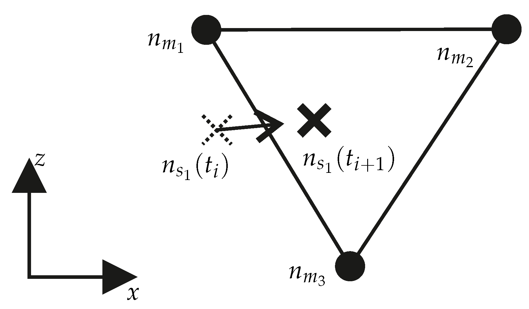Therefore, the friction coefficient of the master surface is used at the position where the slave node is located at time $t_{i+1}$, and thus at the end of the current time increment (see term $I.a$ in Equation (18)). By formulating the surface as R3D3 elements, the node $n_{s_j}$ is located on a triangular surface, which is defined by the nodes of the master surface $n_{m_k}\forall k\in M_j$ as shown in Figure 10.

$M_j$ describes the set of all master nodes defining the area where the slave node $n_{s_j}$ is located at time $t_{i+1}$. The coefficient of friction ${\overline{\mu }}_{m_j}\left(t_i\right)$ as a description for term $I.a$ from Equation (18) can be approximated as the mean value of the coefficients of friction at the three adjacent master nodes and is therefore

$$\begin{array}{c}\hfill {\overline{\mu }}_{m_j}\left(t_i\right)=\frac{1}{3}\sum _{k\in M_j}{\mu }_{m_k}\left(t_i\right).\end{array}$$

(25)

A weighting of the values of ${\mu }_{m_k}\forall k\in M_j$ corresponding to their distance to $n_j$ was not done to reduce the complexity of the model.${\mu }_{ini{t}_j}\left(t_i\right)$ thus describes the new coefficient of friction by transporting a part of the viscous residual water film with the slip velocity ${\overrightarrow{v}}_s$ and leaving the other part of the residual water film on the road surface. This coefficient of friction now changes due to further squeezing of the water film, which is described by term $II$ from Equation (24). For the surface pressure ${\overline{p}}_j\left(t_{i+1}\right)$ at the slave node $n_{s_j}$$p_k={\overline{p}}_j\left(t_{i+1}\right)$ applies and thus for the characteristic time at node $n_{s_j}$

$$\begin{array}{cc}\hfill {\tau }_j\left(t_i\right)& =-\frac{1}{-\lambda {\overline{p}}_j\left(t_{i+1}\right)}ln\left(\frac{{\mu }_{ini{t}_j}\left(t_i\right)-{\mu }_{\infty }}{{\mu }_{\infty }-{\mu }_0}\right)\hfill \end{array}$$

(26)

applies. Due to the predefined implementation of the subroutine vfric by Abaqus, the surface pressure $p_j\left(t_{i+1}\right)$ at the end of the current time increment is used to calculate the friction coefficient gradient using the characteristic diagram ${\mu }_k(p_k,\tau )$. Physically, this means that first the fluid film is divided between the two surfaces, then the incremental displacement is performed due to the local slip, and finally the squeezing is calculated based on the water film averaged by the incremental displacement. A different order would also be conceivable, but since the model is freely parameterized anyway, this is not of further importance. Thus, the friction coefficient ${\mu }_{s_j}\left(t_{i+1}\right)$ is completely defined and is used for the calculation of the friction force at the corresponding slave node. This new friction value will be stored for all slave nodes $n_{s_j}$ until the next time step and will be used again as ${\mu }_{s_j}\left(t_i\right)$ in the next time step. This data can be stored within the subroutine in the statev variable provided by Abaqus. Furthermore, in the next time step a value for ${\mu }_{m_k}\left(t_i\right)$ is needed again (see Equation (24)), which is why the calculated value of ${\mu }_{s_j}\left(t_i\right)$ is also stored proportionally in ${\mu }_{m_k}\left(t_{i+1}\right)$. 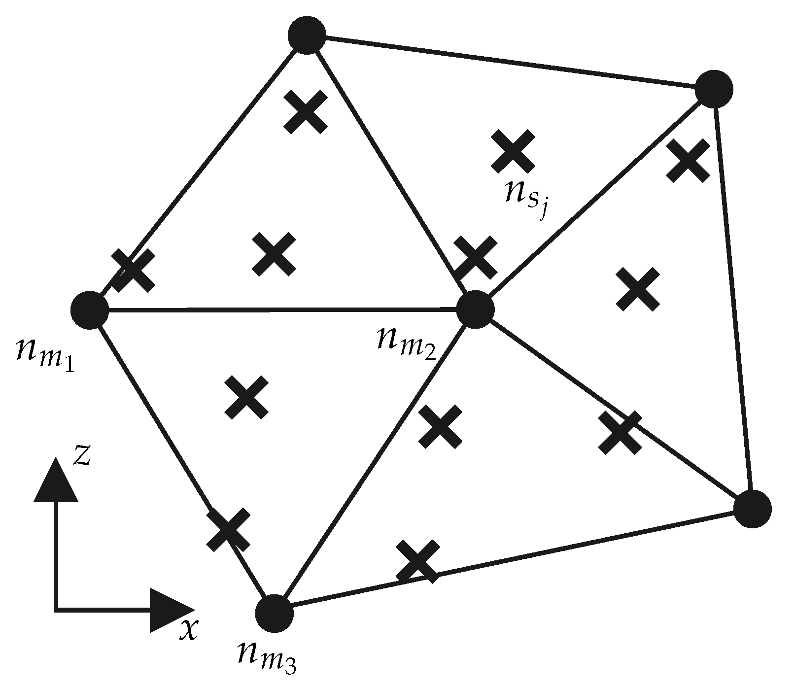The formulaic description is

$$\begin{array}{c}\hfill {\mu }_{m_k}\left(t_{i+1}\right)=\frac{1}{\mathrm{number}(j\in S_k)}\sum _{j\in S_k}{\mu }_{s_j}\left(t_{i+1}\right),\end{array}$$

(27)

where $S_k$ describes the set of all slave nodes that are located at time $t_{i+1}$ on one of the areas defined by $n_{m_k}$. This relationship is shown in Figure 11. Since there are several slave nodes on the areas defined by $n_{m_k}$, the new friction value ${\mu }_{m_k}\left(t_{i+1}\right)$ for a master node is calculated as the average of the friction values ${\mu }_{s_j}\left(t_{i+1}\right)\forall j\in S_k$ of all slave nodes directly adjacent at time $t_{i+1}$. This means that at the end of each time increment the friction coefficient vectors ${\overrightarrow{\mu }}_s$ and ${\overrightarrow{\mu }}_m$ approximate the same course of a real friction coefficient $\mu (x,y,t_{i+1})$ in space. A weighting of the values of ${\mu }_{s_j}\forall j\in S_k$ corresponding to their distance to $m_k$ was omitted analogous to Equation (25). Alternatively, it would also be possible to use only the four slave nodes that form the segment of the slave surface with which the master node $n_{m_k}$ is in contact. Which of these four nodes are in contact cannot be determined directly from the subroutine. Therefore, the coarser approach of the mean value of all Slave nodes located on an area defined by $n_{m_k}$ is chosen here. The storage of ${\mu }_{m_k}\left(t_{i+1}\right)$ is not provided in Abaqus and is therefore carried out in Fortran 77 via a storage location for global variables (Common block).

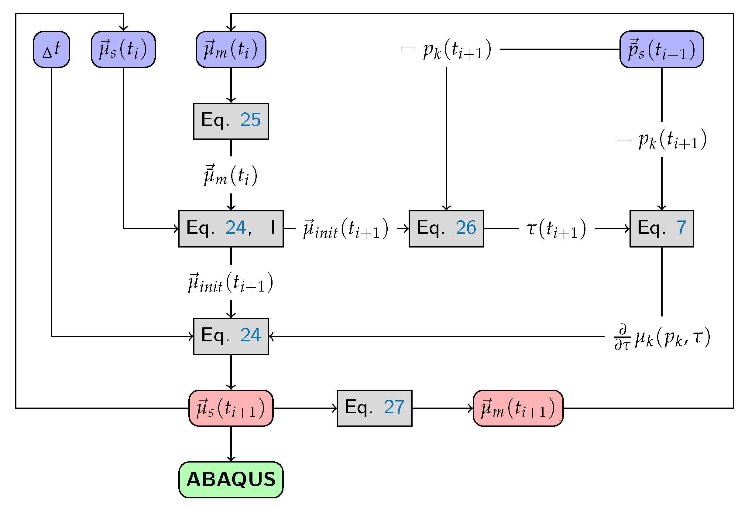
Figure 12 shows the program flow of the subroutine vfric. First, Equation (25) is used to calculate the friction value ${\overrightarrow{\overline{\mu }}}_m$ on the master interface. The result is used in Equation (24), part I together with the friction value on the slave surface ${\overrightarrow{\mu }}_s\left(t_i\right)$ to calculate the initial friction value ${\overrightarrow{\mu }}_{init}$. Thus, according to Equation (26) using ${\overrightarrow{\overline{p}}}_s$, the characteristic time $\tau$ can be calculated, which in turn is used in Equation (7) to read out the gradients $\partial {\mu }_k·\partial {\tau }^{-1}$. This allows the friction value ${\overrightarrow{\mu }}_s\left(t_{i+1}\right)$ to be determined in Equation (24), which is used by Abaqus to calculate the friction forces. Within the subroutine, the friction value ${\overrightarrow{\mu }}_m\left(t_{i+1}\right)$ is then stored to the corresponding master node using Equation (27).

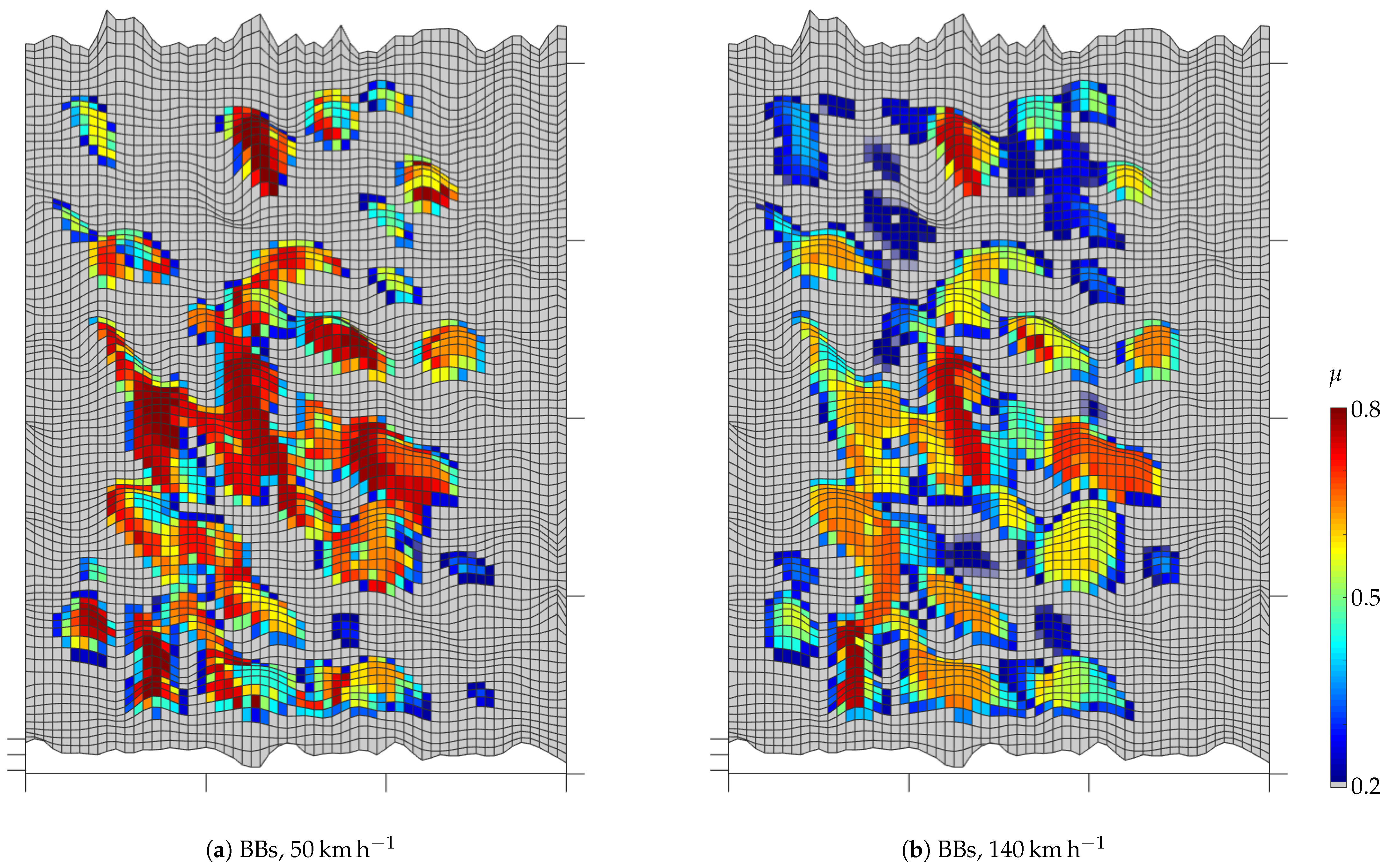
Figure 13 shows the local coefficient of friction on the road surface at the end of simulation for pattern BBs. Where no contact is established, the viscous water film remains undisturbed and the coefficient of friction is equal to ${\mu }_0$. On the roughness peaks the water film has been squeezed out and the coefficient of friction ${\mu }_{\infty }$ is present. On flatter elevations, where lower contact pressures have prevailed, the coefficient of friction is between ${\mu }_0$ and ${\mu }_{\infty }$. At 50 $\mathrm{k}$$\mathrm{m}$ ${\mathrm{h}}^{-1}$ the tread block was longer in the tire contact area and therefore more time was available to squeeze out the water. This is reflected in the slightly higher overall friction coefficient level. It should be noted that the sliding path covered by the tread block during the simulation is independent of the driving speed, since the sliding speed is directly proportional to the driving speed, which in turn is inversely proportional to the contact time.

In some cases, areas can be seen where the coefficient of friction at 140 $\mathrm{k}$$\mathrm{m}$ ${\mathrm{h}}^{-1}$ is higher than at 50 $\mathrm{k}$$\mathrm{m}$ ${\mathrm{h}}^{-1}$. On the one hand, the overall greater dynamics of the tread block movement at 140 $\mathrm{k}$$\mathrm{m}$ ${\mathrm{h}}^{-1}$ can lead to contact being established briefly in some areas where there would otherwise have been no contact at all between the rubber and the road surface. This can be seen in the top right of Figure 13b. On the other hand, the material damping in the rubber can lead to locally higher contact pressures and thus to a faster increase in the coefficient of friction. Both effects are negligible for the global friction force.

3.2.3. Wiping Edge

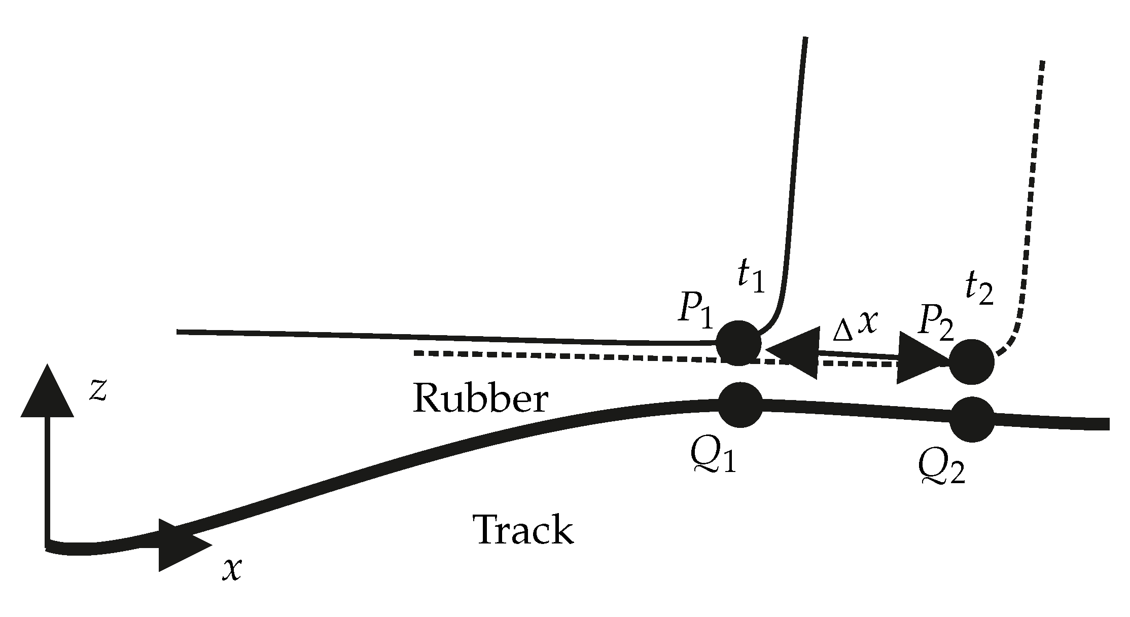
As an extension of the friction law, a so-called wiping edge effect was modeled. The model idea is that an edge of the tread block does not float on the viscous residual water film in front of it, but wipes it away. Since a high coefficient of friction is quickly established under an edge due to the high surface pressure, this is carried along when the edge slips over the road surface. This is illustrated in Figure 14.

At the time $t_1$ a certain coefficient of friction is present at the points $Q_1$ and $P_1$. At point $P_2$ there is the initial friction value ${\mu }_0$. Up to time $t_2$$Q_1$ now slides to the right by the distance ${}_{\Delta }x$. Instead of forming the mean value of the friction values at $Q_1$ and $P_2$ according to Equation (24), the following now applies for term I of Equation (24)

$$\begin{array}{c}\hfill {\mu }_{ini{t}_j}\left(t_i\right)={\overline{\mu }}_{m_j}\left(t_i\right).\end{array}$$

(28)

So that we ignore the low coefficient of friction or high viscous residual water film at $P_2$ and use the higher coefficient of friction of $Q_1$ instead. Whether it is really an edge is checked in the simulation using two conditions. First, the friction value at the slave node at the beginning of the time step must be higher than on the master surface. The condition for this is

$$\begin{array}{cc}\hfill {\overline{\mu }}_{m_j}\left(t_i\right)& >={\alpha }_w{\overline{\mu }}_{s_j}\left(t_i\right).\hfill \end{array}$$

(29)

Physically, this means that the edge slides from a dry area of the roadway back onto a wet part of the roadway. Accordingly, the coefficient of friction on the master surface would be lower than on the slave node. However, Equation (28) adjusts this to the friction coefficient at the slave node and the water film in front of the edge is thus ’wiped away’. The threshold value ${\alpha }_w$ ensures that minor irregularities in the friction coefficient curve are not mistakenly classified as an edge. In addition, the condition

$$\begin{array}{c}\hfill {\mu }_{m_k}\left(t_i\right)={\mu }_0\end{array}$$

(30)

must be fulfilled for at least one $k\in M_j$. This means that at least one node of the road segment on which the master node $n_{s_j}$ is currently located must have the initial friction value ${\mu }_0$, which corresponds to an undisturbed viscous residual water film at this node. If this condition is not fulfilled, all neighboring nodes of the master were already in contact at an earlier time and there is no undisturbed viscous residual water film that could be wiped away from the tread block edge. A restriction of the nodes that could be considered to be edges to certain areas was not carried out due to the sometimes very large tread block deformations. In principle, every node of the tread block can be identified as an edge, as long as the conditions from Equations (28) and (30) are fulfilled.

In Figure 15 all nodes of the roadway are shown on which the wiping edge effect was detected until the end of the simulation. The color scale marks the friction coefficient change caused by the wiping edge effect according to Equation (28). Apart from a few false detections, the 4 edges of pattern BBs (b), or individual edges of pattern BB (a) are clearly visible. In pattern BBs, the front edge is much more pronounced than the three following edges. This is due to the fact that from a certain point in time the rear edges slip over areas of the carriageway on which the water film has already been squeezed out by the preceding block segment. Thus, Equation (30) is not fulfilled and no wiping edge effect is detected. Nevertheless, there is a high coefficient of friction in this area, as can be seen in Figure 13b.

3.2.4. Block Tilting and Hysteresis

Due to the macro-roughness of the road surface, it is possible that the edges of the tread blocks get caught on individual roughness peaks. This causes a crosstalk of the normal force into the circumferential force, which is why the global friction coefficient, determined according to Equation (1), can theoretically be greater than the local limit friction coefficient ${\mu }_{\infty }.$ Another reason for this is that the model maps hysteresis friction due to the damping losses in the rubber material. Actually, hysteresis friction should be modeled by the friction law, but the combination of damping material properties and macro-rough pavement leads to directly modeling hysteresis friction on the largest length scale of track roughness. Corresponding simulations have shown that damping in the material law cannot be dispensed with, since otherwise, on the one hand, the dynamic behavior of the model becomes very unstable and, on the other hand, no realistic contact areas and contact pressures are calculated. These quantities are of elementary importance for the friction law and the reason the roadway is modeled as a three-dimensional structure with full macro-roughness at all. Therefore, when interpreting the results later, it must be taken into account that they not only reflect the influence of the friction law, but also include hysteresis friction on the largest length scale.

3.2.5. Loss of Contact

If a node of the tread block loses contact with the road surface, the friction value at the corresponding slave node is reset to the initial friction value ${\mu }_0$. In this case, a rubber element slides from one asperity over a valley in the roadway to the next asperity. During the time of loss of contact, the rubber surface can be wetted with water again, so it is not useful to continue calculating with the coefficient of friction from the last contact. Conversely, however, it is assumed that a roughness peak retains its coefficient of friction even if contact with the rubber is lost in the meantime. A backflow of the fluid on tips that have been drained at once is therefore not permitted. Physically, there is no reason the fluid should flow back to a single peak, against the force of gravity and within the very short time of only a few milliseconds.

3.2.6. Self-Contact

Due to the strong local deformations of the rubber, especially for the laminated pattern BBs, self-contact of the rubber can occur. This contact is formulated identically to that between the rubber and the road surface; however, a constant coefficient of friction of ${\mu }_r$ = 0.2 is applied. Since the individual slats on their upper side are all fixed at the same height and all have the same length, which is much greater than the distance between the slats, only very small tangential displacements occur between adjacent slats at the contact points. Therefore, the height of the coefficient of friction at this point is of secondary importance. The relatively low value of ${\mu }_r$ = 0.2 was chosen because squeezing a water film between two macro smooth surfaces at low surface pressure takes a very long time and tangential forces are therefore probably only transmitted via the viscosity of the fluid. The decisive factor is rather that the individual lamellae do not penetrate each other but support each other. This phenomenon can also be seen in Figure 8 between the first and second lamella. To secure the choice of the parameter, simulations with ${\mu }_r$ = 0.1 to 0.3 were carried out. In this case, the mean braking force changes only by a few per mile for pattern BBs. Also, the temporal progressions of braking force and contact surface between pattern BBs and road surface are almost identical. For patterns BB and SB, the results are, as expected, independent of ${\mu }_r$, since there is at best very local self-contact.

3.3. Parameterization

The local friction law forms the influence of the viscosity of the fluid as intermediate medium in the contact area of the rubber with the roughness peaks of the road surface. The parameters to be defined are ${\mu }_0$, ${\mu }_{\infty }$ and $\lambda$. For each material pairing of rubber and road surface a set of parameters must be defined which describes the micro-roughness of the road surface, the size and distribution of asperites, the viscosity of the fluid as well as the coefficient of friction of the corresponding material pairing. For the parameterization, the measurement results of brake tests with the patterns BB and BBs are used. The results of 1 $\mathrm{m}$$\mathrm{m}$ water level and 50 $\mathrm{km}$ $\mathrm{h}$⁻¹ or 140 $\mathrm{km}$ $\mathrm{h}$⁻¹ driving speed are used.

The quality criteria are the sum of the least squares of errors regarding the deviation between model and test result and the correlation between model and test result. The parameter space in question was defined by preliminary simulative investigations and is shown for the asphalt and safety-walk pavements as summarized in

Table 5. Representation of the reasonable ranges for the parameters freely selectable in the model on the investigated asphalt track.

Parameter	Range
${\mu }_0$/-	0.2
${\mu }_{\infty }$/-	0.6…0.9
$\lambda$$/{\mathrm{MPa}}^{-1} {\mathrm{s}}^{-1}$	$100\dots 1000$

.

The initial friction value ${\mu }_0$ represents the viscous friction at the moment of first contact on a macroscopic level. At this point in time, the viscous residual water film is still closed, and forces are transmitted exclusively via the shear of the fluid. Therefore, this parameter is set to ${\mu }_0$ = 0.2 in the following. The limit coefficient of friction ${\mu }_{\infty }$ describes the maximum locally achievable coefficient of friction and should therefore be set in a similar range to the measured global coefficient of friction. The most important parameter is $\lambda$, which as a unit has the reciprocal of the dynamic viscosity. If it is chosen too large, the limit friction value ${\mu }_{\infty }$ is established everywhere in the contact within a very short time, which corresponds to a constant friction value without the influence of a fluid. In this case, the model predicts neither a velocity nor a pattern dependence of the global coefficient of friction at the tread block. If it is chosen too small, the contact time within a latching run of the tread block is not sufficient to displace the viscous residual water film and viscous aquaplaning occurs, as would be expected, for example, on an oil-covered road. The parameter space shown in Table 5 is scanned full-factorially to parameterize the model according to the test results.

4. Results

In this section, the basic model results are discussed and checked for plausibility. The parameterization of the model as shown in

Table 6. Model parameters for the friction law.

${\mathit{\mu }}_{\mathit{\infty }}$/-	${\mathit{\mu }}_0$/-	$\mathit{\lambda }$/MPa${}^{-1}$ s${}^{-1}$	Track
0.8	0.2	600	asphalt

is used. The choice of these parameters is explained in Section 5 and is taken as given here. The model validation based on the measurement results is also explained in Section 5.

Figure 16a shows the temporal progression of the specified normal force at the top of the block and the resulting normal and longitudinal force in contact. Despite the slowly increasing load $F_z\left(t\right)$, which acts as a ramp function, the block hits the road relatively abruptly and is thus excited to oscillations in vertical direction, which decay within 1 $\mathrm{m}$$\mathrm{s}$, and thus relatively quickly, due to the material damping. These oscillations become apparent in the contact forces $F_N\left(t\right)$ and $F_x\left(t\right)$. If the global friction coefficient shown in Figure 16b is calculated from the contact forces according to Equation (1), these overshoots are largely compensated. The mean value of this coefficient of friction serves as a descriptive variable for the transmittable braking forces of the investigated pattern at the given parameters and is later used to validate the model.

Depending on the driving speed and relative slip, the absolute slip speed $v_s$ is given at the top of the block (see Figure 3). If the slip is varied for one speed, one of the $\mu$-slip curves shown in Figure 17 will result. The other curves are the result of simulations with the same parameters, but the block has been displaced by 20 $\mathrm{m}$$\mathrm{m}$ on the track in the direction of travel. Each of the points drawn is therefore the result of a separate simulation with constant slip. All simulations on the same point of the pavement are connected to form a curve. It can be seen that for all positions there is a maximum in the range between 5% and 7.5% slip. This is also the range in which the maximum of the $\mu$-slip curves was measured during the brake tests with a complete tire presented in Section 2. In the model, a certain amount of slip is necessary to shear the tread block and thus build up longitudinal forces. At high slip speeds, the coefficient of friction decreases again due to the time component of the friction law. The greater the distance covered by the tread block, the greater the area of the roadway on which the viscous residual water film must be displaced within the contact time. At a constant coefficient of friction $\mu ={\mu }_{\infty }$ on the road surface, the global coefficient of friction would continue to increase with increasing slip, since more energy would be dissipated due to material damping. It can be clearly seen that the choice of position on the road has a great influence on the result, which is not the same for all slip values. Therefore, the choice of a representative road position is not possible and in the following the mean value of simulations on five different road positions is used.

Figure 18 shows the $\mu$ over slip curves for patterns BB and BBs. The larger geometric stiffness of pattern BB compared to pattern BBs is clearly visible in the slope of the curves from zero. Since the laminated block can deform more and the water is pressed out faster due to the higher surface pressure, the curve only reaches its maximum at a higher slip. In addition, the higher maximum value for pattern BBs can be seen. This is also based on a faster increase in the local coefficient of friction due to the higher local surface pressure. The coefficient of friction for 0% slip was not calculated, but assumed to be zero and manually added to the diagram for a better visualization of the initial slope.

5. Validation

The first question is which measurements can be used to validate the wet grip model. In Figure 19 measurement results of the complete tires on the internal drum test bench are shown at 120 $\mathrm{k}$$\mathrm{m}$ ${\mathrm{h}}^{-1}$ on a damp road and at 1 $\mathrm{m}$$\mathrm{m}$ water level. For pattern BB the results are almost identical. For pattern BBs and SB, the coefficient of friction at 1 $\mathrm{m}$$\mathrm{m}$ is even higher than on damp pavement. This indicates that even at 1 $\mathrm{m}$$\mathrm{m}$ the inertia of the water plays only a minor role. A possible explanation for the poorer performance on damp pavement is the influence of temperature. The lower the geometric stiffness of the pattern, the worse the result with a damp pavement compared to 1 $\mathrm{m}$$\mathrm{m}$. Due to the strong deformation of the rubber, locally higher contact pressures and thus higher temperatures are achieved, which in turn can lead to a reduction of the hysteresis component. Due to the constant water supply during the measurements with 1 $\mathrm{m}$$\mathrm{m}$, the total road and tire temperature is lowered, so that this effect is reduced. It can therefore be assumed that wet grip effects are dominant at 1 $\mathrm{m}$$\mathrm{m}$ and at the same time an excessive temperature influence is avoided, which is why the measurements at 1 $\mathrm{m}$$\mathrm{m}$ water level are used for model validation.

First the model parameters ${\mu }_{\infty }$ and $\lambda$ must be determined. They are selected so that the best possible approximation to the test results is achieved for patterns BB and BBs at 1 $\mathrm{m}$$\mathrm{m}$ water level. This results in the parameters already shown in Table 6. For this purpose, the parameter space shown in Table 5 was searched full-factorially with increments of ${}_{\delta }{\mu }_{\infty }=0.1$ and ${}_{\delta }\lambda =100 {\mathrm{MPa}}^{-1} {\mathrm{s}}^{-1}$. Finally, the combination of parameters is used which provides the best correlation between model and test and at the same time minimizes the sum of the error squares. The selection was made manually. Due to the relatively large scatter in the test results, a more extensive and automatic optimization of the model parameters was not found useful. Instead, the aim was to map the most important effects regarding pattern and speed influence at a realistic friction coefficient level. In addition, the model behaves relatively linear with small changes of ${\mu }_{\infty }$ and the exact position of the absolute friction coefficient level could thus be adjusted by a corresponding adjustment of ${\mu }_{\infty }$ without significantly changing the correlation between measurement and model.

Figure 20 shows the simulation results of the wet grip model for the parameters shown in Table 6. The relative slip was set to $7.5\%$. This is the range in which ${\mu }_{max}$ was measured during brake tests and the maximum of most simulated $\mu$-slip curves. This is also the range in which the maximum of the friction coefficients measured during ABS braking is observed ([34], [p. 25]). For comparison, the test results are shown at 1 $\mathrm{m}$$\mathrm{m}$ water level.

The decrease over speed is slightly smaller for pattern BBs than for patterns BB and SB. Although the test results point in the same direction, the increasing grip level for pattern BBs is not considered to be plausible and will not be further discussed. In contrast, the higher level of friction for pattern BBs is clearly visible in the model. This is mainly due to the local friction law from Section 3.2.2, which rewards the higher local contact pressures by a faster squeezing of the viscous residual water film. To confirm this hypothesis, Figure 21 shows the progression of the contact area and the global coefficient of friction over time. Again, the mean value of the curves calculated for five different road positions was calculated. The course of $\mu$ over the speed is almost linear for all patterns, which is why only the speeds of 50 $\mathrm{k}$$\mathrm{m}$ ${\mathrm{h}}^{-1}$, 100 $\mathrm{k}$$\mathrm{m}$ ${\mathrm{h}}^{-1}$ and 140 $\mathrm{k}$$\mathrm{m}$ ${\mathrm{h}}^{-1}$ were simulated.

The calculated contact areas are not scaled, which is why the contact area of pattern SB is much smaller than the contact area of patterns BB and BBs. For the following argumentation, the change of contact area over time is deciding. For all patterns, overshoot occurs in the contact area after the first contact. Pattern SB then settles down at a relatively constant level, while a slight drop in the contact surface can be observed for pattern BB. Pattern BBs starts with almost the same contact area as pattern BB, but subsequently the setting up of the individual slats leads to a significantly reduced contact area. Since the wheel load remains constant, the surface pressure in contact is correspondingly higher. This is reflected in the global coefficient of friction ${\mu }_G\left(t\right)$ shown on the right, which increases much higher for pattern BBs. The different course only occurs after 1 $\mathrm{m}$$\mathrm{s}$, since the tread blocks must first be deformed by the slip movement. It should also be noted here that the global coefficient of friction is higher than the maximum local coefficient of friction ${\mu }_{\infty }$ due to material damping and edge effects (see Section 3.2.4).

Figure 22 shows a section through the tread blocks of pattern BB and BBs after $1.9$ $\mathrm{m}$$\mathrm{s}$ and $3.8$ $\mathrm{m}$$\mathrm{s}$ respectively. Pattern BB is only slightly deformed and the pressure distribution in the contact changes only slightly due to the slip movement of the tread block. With pattern BBs, it is clearly visible how the second block segment gets stuck on a road elevation. As a result, this segment is strongly deformed, and locally higher contact pressures arise.

Figure 23 shows the coefficient of friction on the road surface after 3 $\mathrm{m}$$\mathrm{s}$. It can be clearly seen that the coefficient of friction for pattern BBs is higher on average and that there is a larger area with a high coefficient of friction.

The model predicts a slightly better performance for pattern BB than for pattern SB. In the test results, both patterns perform almost identically. The reason for the poorer performance of pattern SB could be the smaller block-length of pattern SB. The leading edge is subjected to less stress, which means that there is no canting or curling of the edge. This leads to the strong reduction in contact area for pattern BBs, and the effect is still visible with pattern BB due to the slightly decreasing contact area in Figure 21a.

The error bars on the measured curves in Figure 20 indicate the standard deviation. Due to the measurement inaccuracies alone, complete agreement between model and measurement is not to be expected. Nevertheless, it must be noted that the spread between BB and BBs in the model is limited and cannot be increased arbitrarily even if the model parameters are varied.

In addition, a simulation without the wiping edge effect (see Section 3.2.3) was performed for comparison. A reduction of the global friction coefficient of maximum $0.6\%$ can be observed. The effect of the wiping edge is therefore negligible here, at least compared to the influence of the local contact pressure distribution on the friction law. However, the edge was identified only indirectly, as described in Section 3.2.3, so that a more precise detection of the edges could possibly lead to a somewhat greater influence of the effect.

6. Conclusions

An FE model of a single-tread block was built to investigate the pattern-dependent wet-braking behavior of passenger car tires on an asphalt track. The material properties of the rubber are considered by a viscoelastic and a hyperelastic material law. A three-dimensional image of the road macrotexture reflects the influence of the road surface used in the model. The friction coefficient in the contact area is described by a phenomenological friction law. The underlying idea of the model is that there is initially a thin viscous water film in the contact area, which strongly reduces the local friction coefficient. This is squeezed out by the local surface pressure and the local friction coefficient increases. With this model the much better performance of the siped pattern can be explained, as could be shown by the validation of the model with braking tests on an internal drum test bench. The model presented here allows the consideration of the interactions between a rough road surface, deformable tread blocks and a viscous fluid film at very low water heights. In particular, it should be emphasized that very low water heights were modeled, at which the inertia of the fluid and the drainage of the tire contact patch play a negligible role.

References

1. Persson, B. Sliding friction. Surf. Sci. Rep. 1999, 33, 83–119. [Google Scholar] [CrossRef]
2. Fuller, K.N.; Tabor, D. The effect of surface roughness on the adhesion of elastic solids. Proc. R. Soc. Lond. Ser. A. Math. Phys. Sci. 1975, 345, 327–342. [Google Scholar] [CrossRef] [Green Version]
3. Persson, B.N.J.; Tartaglino, U.; Albohr, O.; Tosatti, E. Sealing is at the Origin of Rubber Slipping on Wet Roads. Nat. Mater. 2004, 3, 882–885. [Google Scholar] [CrossRef] [PubMed] [Green Version]
4. Schramm, E.J. Reibung von Elastomeren auf rauen Oberflächen und Beschreibung von Nassbremseigenschaften von PKW-Reifen. Ph.D. Thesis, Universität Regensburg, Regensburg, Germany, 2002. [Google Scholar]
5. Lindner, M. Experimentelle und theoretische Untersuchungen zur Gummireibung an Profilklötzen und Dichtungen. Ph.D. Thesis, Universität Hannover, Hannover, Germany, 2005. [Google Scholar] [CrossRef]
6. Kummer, H.W. Unified Theory of Rubber and Tire Friction; Pennsylvania State University, College of Engineering: University Park, PA, USA, 1966. [Google Scholar]
7. Moldenhauer, P. Modellierung und Simulation der Dynamik und des Kontakts von Reifenprofilblöcken. In Berichte aus dem Institut für Maschinenelemente, Konstruktion und Fertigung der Technischen Universität Bergakademie Freiberg; VDI Verlag: Düsselorf, Germany, 2010; Volume Nr. 720. [Google Scholar]
8. Mofidi, M.; Prakash, B.; Persson, B.N.J.; Albohr, O. Rubber friction on (apparently) smooth lubricated surfaces. J. Phys. Condens. Matter 2008, 20, 085223. [Google Scholar] [CrossRef] [Green Version]
9. Do, M.T.; Cerezo, V. Road surface texture and skid resistance. Surf. Topogr. Metrol. Prop. 2015, 3, 043001. [Google Scholar] [CrossRef]
10. Busse, L.; Boubakri, I.; Klueppel, M. Friction master curves for rubber on dry and wet granite experiments and simulations. KGK Kautsch. Gummi Kunstst. 2011, 64, 35–39. [Google Scholar]
11. Do, M.T.; Cerezo, V.; Beautru, Y.; Kane, M. Modeling of the connection road surface microtexture/water depth/friction. Wear 2013, 302, 1426–1435. [Google Scholar] [CrossRef]
12. Kane, M.; Cerezo, V. A contribution to tire/road friction modeling: From a simplified dynamic frictional contact model to a “Dynamic Friction Tester” model. Wear 2015, 342–343, 163–171. [Google Scholar] [CrossRef]
13. Kane, M.; Do, M.T.; Cerezo, V.; Rado, Z.; Khelifi, C. Contribution to pavement friction modelling: An introduction of the wetting effect. Int. J. Pavement Eng. 2017, 4, 1–12. [Google Scholar] [CrossRef]
14. Kulakowski, B.T.; Harwood, D.W. Effect of Water-Film Thickness on Tire-Pavement Friction. In Surface Characteristics of Roadways: International Research and Technologies; Meyer, W.E., Reichert, J., Eds.; ASTM International: West Conshohocken, PA, USA, 1990; pp. 50–60. [Google Scholar]
15. Persson, B.N.J. Fluid dynamics at the interface between contacting elastic solids with randomly rough surfaces. J. Phys. Condens. Matter Inst. Phys. J. 2010, 22, 265004. [Google Scholar] [CrossRef] [Green Version]
16. Bruggeman, D.A.G. Berechnung verschiedener physikalischer Konstanten von heterogenen Substanzen. I. Dielektrizitätskonstanten und Leitfähigkeiten der Mischkörper aus isotropen Substanzen. Ann. Phys. 1935, 416, 636–664. [Google Scholar] [CrossRef]
17. Persson, B.N.J. Theory of rubber friction and contact mechanics. J. Chem. Phys. 2001, 115, 3840–3861. [Google Scholar] [CrossRef] [Green Version]
18. Persson, B.N.J. Contact mechanics for randomly rough surfaces. Surf. Sci. Rep. 2006, 61, 201–227. [Google Scholar] [CrossRef] [Green Version]
19. Golden, J.M. A theory of wet road-tyre friction. Wear 1981, 71, 307–331. [Google Scholar] [CrossRef]
20. Greenwood, J.A.; Williamson, J.B.P. Contact of Nominally Flat Surfaces. Proc. R. Soc. A Math. Phys. Eng. Sci. 1966, 295, 300–319. [Google Scholar] [CrossRef]
21. Moore, D.F. The Friction and Lubrication of Elastomers; International Series of Monographs on Materials Science and Technology; Pergamon Press: Oxford, UK, 1972; Volume 9. [Google Scholar]
22. Wagner, P.; Wriggers, P.; Klapproth, C.; Prange, C.; Wies, B. Multiscale FEM approach for hysteresis friction of rubber on rough surfaces. Comput. Methods Appl. Mech. Eng. 2015, 296, 150–168. [Google Scholar] [CrossRef]
23. Wagner, P.; Wriggers, P.; Veltmaat, L.; Clasen, H.; Prange, C.; Wies, B. Numerical multiscale modelling and experimental validation of low speed rubber friction on rough road surfaces including hysteretic and adhesive effects. Tribol. Int. 2017, 111, 243–253. [Google Scholar] [CrossRef]
24. Gnadler, R.; Unrau, H.J.; Fischlein, H.; Frey, M. Ermittlung von mu-Schlupf-Kurven an Pkw-Reifen. FAT-Schr. 1995, 119. [Google Scholar]
25. Fischlein, H. Untersuchung des Fahrbahnoberflächeneinflusses auf das Kraftschlußverhalten von Pkw-Reifen; Fortschritt-Berichte VDI. Reihe 12, Verkehrstechnik/Fahrzeugtechnik; VDI-Verlag: Düsseldorf, Germany, 2000; Volume 414. [Google Scholar]
26. van Oosten, J.; Augustin, M.; Gnadler, R.; Unrau, H.J. EC Research Project TIME—Tire Measurements Forces and Moments. Workpackage 2: Analysis of parameters influencing tyre test results. In Fortschritt-Berichte VDI. Reihe 12; 2. Darmstädter Reifenkolloquium; Breuer, B., Ed.; VDI-Verl.: Düsseldorf, Germany, 1998; Volume 362, pp. 66–83. [Google Scholar]
27. Pacejka, H.B.; Besselink, I. Tire and Vehicle Dynamics, 3rd ed.; Elsevier/BH: Amsterdam, The Netherlands; Boston, MA, USA, 2012. [Google Scholar]
28. Lorenz, B.; Persson, B.N.J. Fluid squeeze-out between rough surfaces: Comparison of theory with experiment. J. Phys. Condens. Matter 2011, 23, 355005. [Google Scholar] [CrossRef] [PubMed] [Green Version]
29. Golfianto, H. Simulation of Rubber Friction on Rough Surface with Abaqus. Master’s Thesis, Karlsruher Institut für Technologie-Institut für Fahrzeugsystemtechnik-Teilinstitut Fahrzeugtechnik-Institutsbibliothek-19-F-0043, unv., Karlsruhe, Germany, 15 May 2019. [Google Scholar]
30. Simulia. Abaqus Materials Guide (2018), o.J. Available online: https://www.3ds.com/products-services/simulia/services-support/support/documentation/ (accessed on 20 February 2021).
31. Wagner, P. A multiscale FEM approach for rubber friction on rough surfaces. Ph.D. Thesis, Leibniz Universität Hannover, Hannover, Germany, 2018. [Google Scholar]
32. Blatz, P.J.; Ko, W.L. Application of Finite Elastic Theory to the Deformation of Rubbery Materials. Trans. Soc. Rheol. 1962, 6, 223–252. [Google Scholar] [CrossRef] [Green Version]
33. Simulia. Abaqus User Subroutines Guide (2018), o.J. Available online: https://www.3ds.com/products-services/simulia/services-support/support/documentation/ (accessed on 20 February 2021).
34. Le Gal, A. Investigation and modelling of rubber stationary friction on rough surfaces. Ph.D. Thesis, Gottfried Wilhelm Leibniz Universität Hannover, Hannover, Germany, 2007. [Google Scholar] [CrossRef]
Figure 1. Schematic representation of the pattern geometries For detailed information see Appendix A. The direction of travel is vertical. (a) Big blocks (BB). (b) Big blocks with sipes (BBs). (c) Small blocks (SB).
Vehicles 03 00006 g001
Figure 2. Schematic diagram of the internal drum test rig with water supply (a), capacitive water level sensor (b), wheel guide (c), drum bearing (d) and road surface (e). The arrows mark the direction of rotation of drum and tire.
Vehicles 03 00006 g002
Figure 3. Representation of the contact between tread block and rough road surface. The thick blue line represents the area of the viscous water film, μ ( x , y , t ) the time and location dependent coefficient of friction prevailing in the contact.
Vehicles 03 00006 g003
Figure 4. Exemplary course of the coefficient of friction μ ( x , y , t ) over time at a certain position x 1 , y 1 for constant values of μ , μ 0 , a temporal constant local surface pressure p ¯ ( x 1 , y 1 ) and different values of λ , where λ 1 > λ 2 > λ 3 .
Vehicles 03 00006 g004
Figure 5. Extract from the friction coefficient map μ k ( p k , τ ) for the local contact pressure p ¯ ( x , y , t i ) = p k currently applied to a fixed point x , y . With the currently applied real coefficient of friction μ ( x , y , t i ) = μ k the characteristic time τ ( x , y , t i ) can be determined and thus again the gradient μ k · τ 1 | τ ( x , y , t i ) .
Vehicles 03 00006 g005
Figure 6. Fixed inertial coordinate system x , y and rubber fixed relative coordinate system x , y . The vector r indicates the shift of the relative coordinate system with respect to the inertial system.
Vehicles 03 00006 g006
Figure 7. Velocity distribution over the water film height h v assuming a Poiseuille flow (left). Approximated binary velocity distribution with equivalent volume flow (right).
Vehicles 03 00006 g007
Figure 8. FE model with the roadway as master and the tread block as slave. A T o p is the top side of the tread block.Illustration FE Model
Vehicles 03 00006 g008
Figure 9. Storage module E and loss module E for a rubber material as a function of frequency ω (material m1 from ([31], [Appendix C])).
Vehicles 03 00006 g009
Figure 10. The node n s 1 is located at time t i + 1 on a triangular area which is defined by the nodes n m k k M 1 = n m 1 3 of the master surface.
Vehicles 03 00006 g010
Figure 11. The position of the master node n m 2 and the directly neighboring master nodes at time t i . In addition, the position of all slave nodes which are located at time t i + 1 on areas connected to n m 2 .
Vehicles 03 00006 g011
Figure 12. Program flow of the subroutine vfric.
Vehicles 03 00006 g012
Figure 13. Local friction coefficient on the road surface at the end of the simulation for pattern BBs at 7.5 % slip. A 60 mm × 80 mm large section of the roadway is shown. Direction of travel is from left to right.
Vehicles 03 00006 g013
Figure 14. Schematic diagram of wiping edge effect.
Vehicles 03 00006 g014
Figure 15. Change of the coefficient of friction Δ μ due to the wiping edge effect. A 60 mm × 80 mm large section of the roadway is shown. Direction of travel is from left to right.
Vehicles 03 00006 g015
Figure 16. Simulation results for pattern BB at 140 k m h 1 and the parameters described in Table 6.
Vehicles 03 00006 g016
Figure 17. Variation of slip and road position for pattern BB at 140 k m h 1 . The positions are each displaced 20 m m relative to each other in the direction of travel.
Vehicles 03 00006 g017
Figure 18. Simulated μ -slip curves for patterns BB and BBs at 140 k m h 1 .
Vehicles 03 00006 g018
Figure 19. Comparison wet and 1 m m water height on asphalt at 120 k m h 1 .
Vehicles 03 00006 g019
Figure 20. Comparison of the wet grip model with the measurement results at 1 m m water level on asphalt.
Vehicles 03 00006 g020
Figure 21. Simulation results for pattern BB at 140 k m h 1 and the parameters described in Table 6.
Vehicles 03 00006 g021
Figure 22. Deformed tread blocks for patterns BB (a) and BBs (b) at 140 k m h 1 . The color scale indicates the Mises equivalent stress and covers the same range of values for all representations.
Vehicles 03 00006 g022
Figure 23. Local coefficient of friction on the road surface after 3 m s at 140 k m h 1 for the patterns BBs and BBs.
Vehicles 03 00006 g023