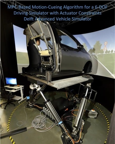
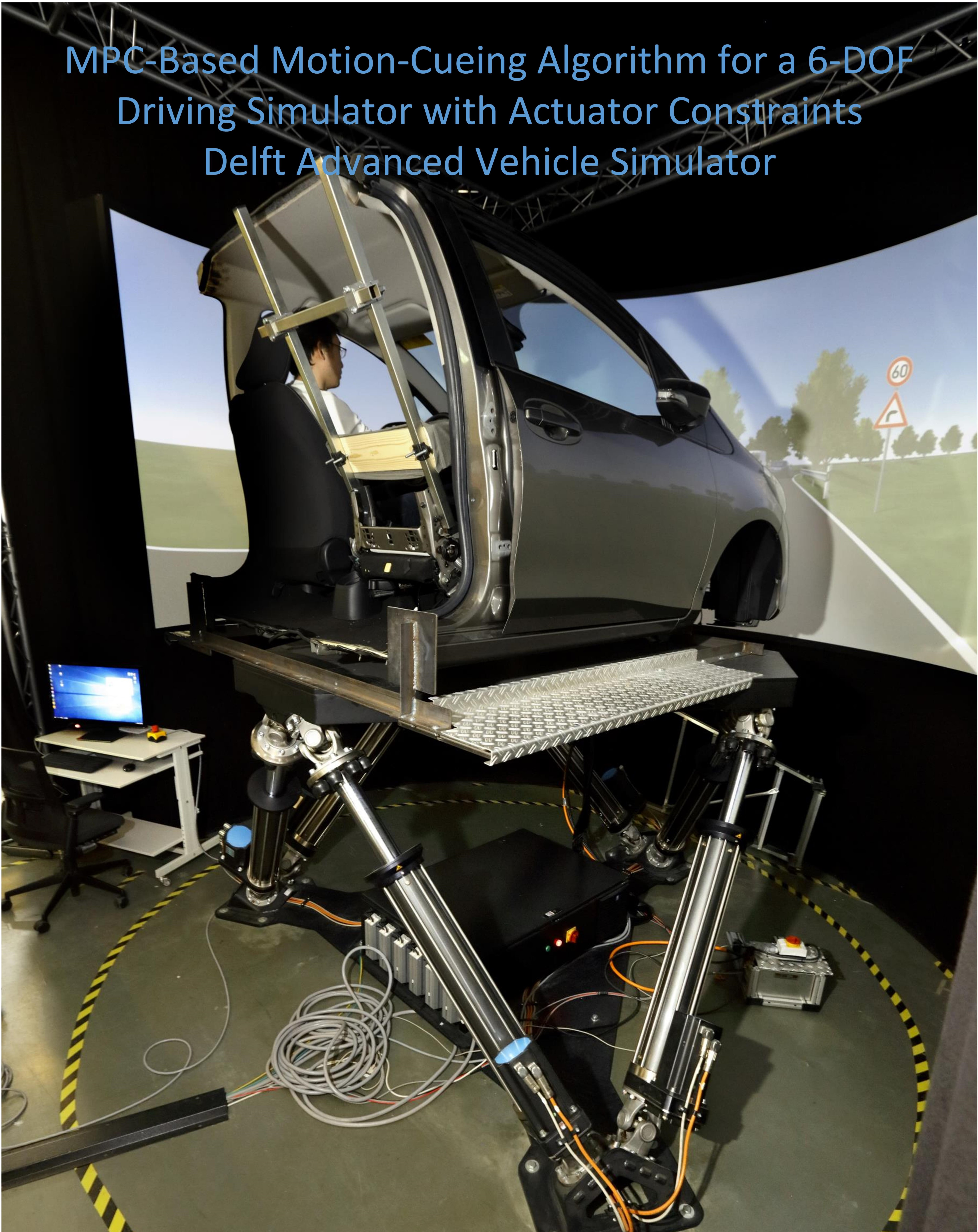
MPC-Based Motion-Cueing Algorithm for a 6-DOF Driving Simulator with Actuator Constraints


Abstract
1. Introduction
- Providing realistic motion cues to the driver or passenger sitting inside the simulator.
- Keeping the motion platform within its physical boundaries.
- Since the parameters of the filters are fixed, they must be designed for the worst-case maneuver. As a result, the algorithm does not use the available workspace for gentle maneuvers resulting in minimum motion.
- Tuning the filters is a complex task because the filter coefficients should be modified based on subjective participant feedback without taking into account meaningful physical quantities.
- Since there is no provision for incorporating the physical limits of the motion platform within the algorithm, the filters have to be tuned for each maneuver/participant to ensure that the motion platform remains within its physical limit.
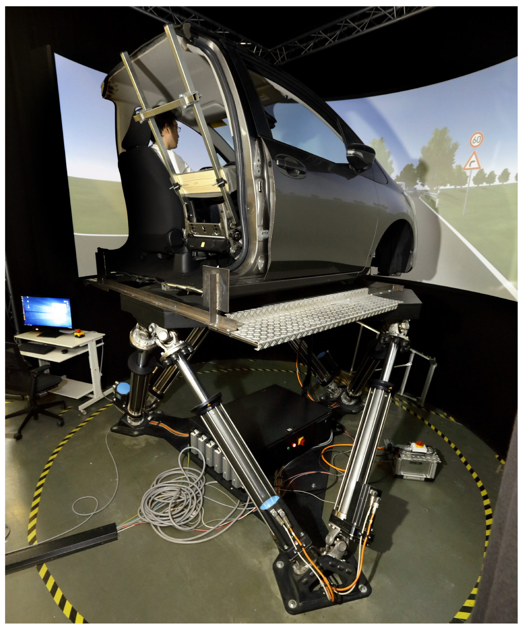
2. Motion Platform
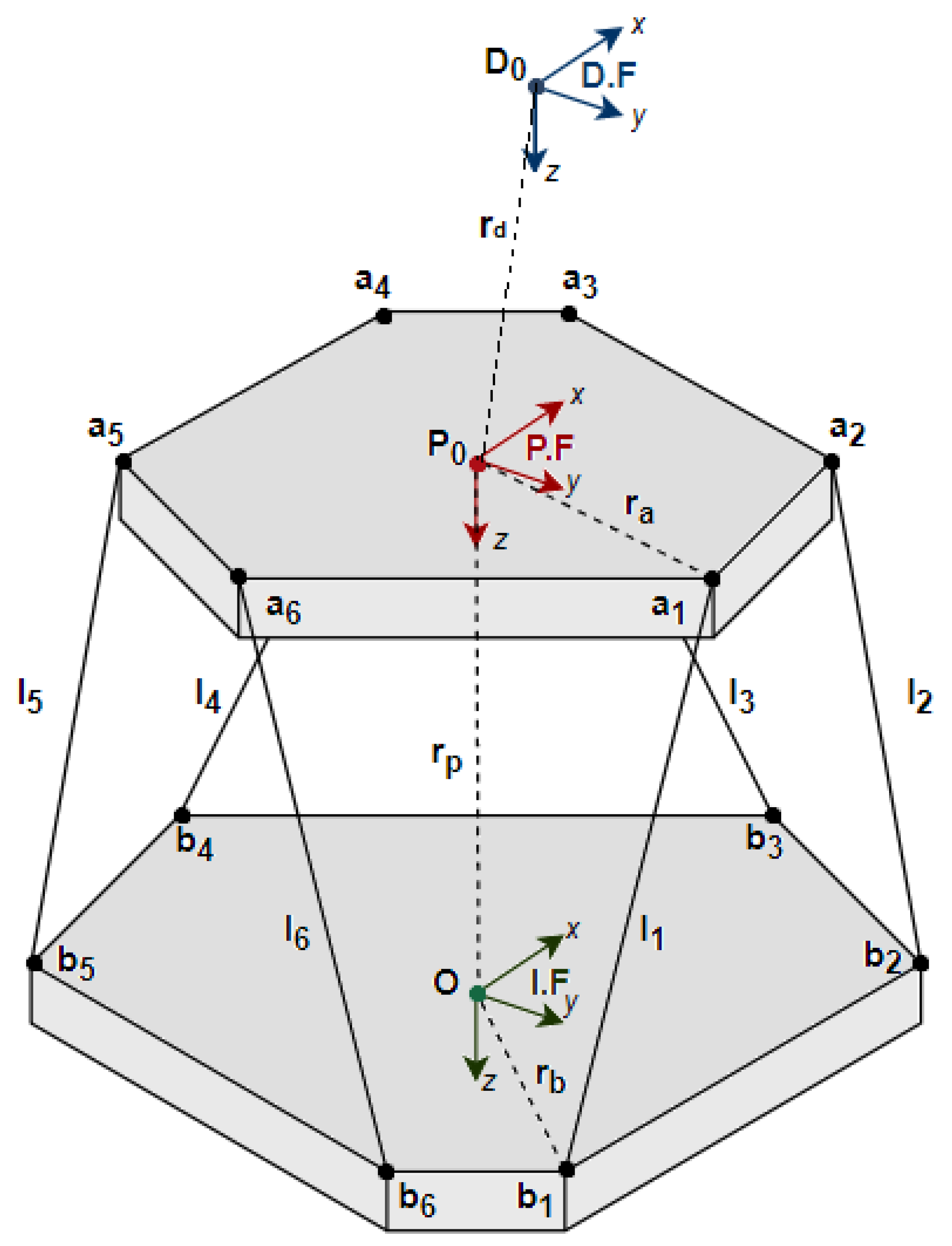
- Inertial Frame (IF)—is fixed to the ground and does not move with the motion platform. The origin coincides with the centroid of the fixed base of the platform (Point O in Figure 4). The positive x-axis points forward, in the direction of drive. The positive y-axis points to the right, while the positive z-axis points vertically downwards.
- Platform Frame (PF)—is fixed to the motion platform and moves with it. The origin coincides with the centroid of the moving plate (Point in Figure 4). Similar to the IF, the positive x-axis points forward, the positive y-axis points to the right, while the positive z-axis points in the downwards direction. Since the PF is body-fixed, its axes are only aligned with that of the IF when the platform has a zero roll, pitch and yaw angle.
- Driver Frame (DF)—is fixed to the driver’s head and moves with it. The origin coincides with the eyepoint of the driver (Point in Figure 4). The positive x-axis points forward, the positive y-axis points to the right, while the positive z-axis points in the downwards direction. Since DF is fixed to the driver’s eyepoint, its axes are only aligned with the IF when the platform has a zero roll, pitch and yaw angle.
3. System Model
- Vestibular system model to provide realistic motion cues.
- Motion platform model to manage the available motion workspace.
3.1. Vestibular System Model
3.1.1. Semi-Circular Canals
3.1.2. Otolith Organ
3.1.3. Complete Vestibular System Model
3.2. Motion Platform Model
- Limiting motion workspace —Forward kinematics is used to calculate the motion space (as per the current actuator position) in terms of the translational and angular displacement of the point . Furthermore, the constraints are applied based on the current motion state and the same should be updated at each time step. As a result, the resulting motion space is a 6-dimensional complex body.
- Limiting actuator workspace—Inverse kinematics is used to determine the motion space directly in terms of the actuator positions. Subsequently, fixed constraints are added based on the permissible actuator length.
Actuator Kinematics
3.3. Combined System Model
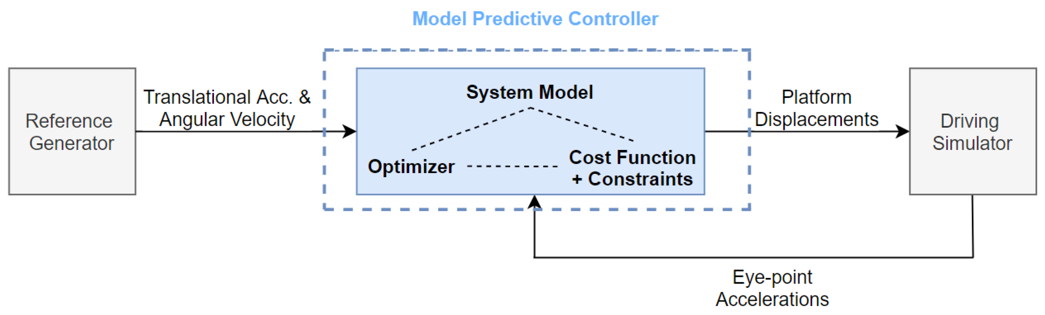
4. MPC Formulation
4.1. Objective Function
4.2. Constraints
- Constraint on the tilt rate ().
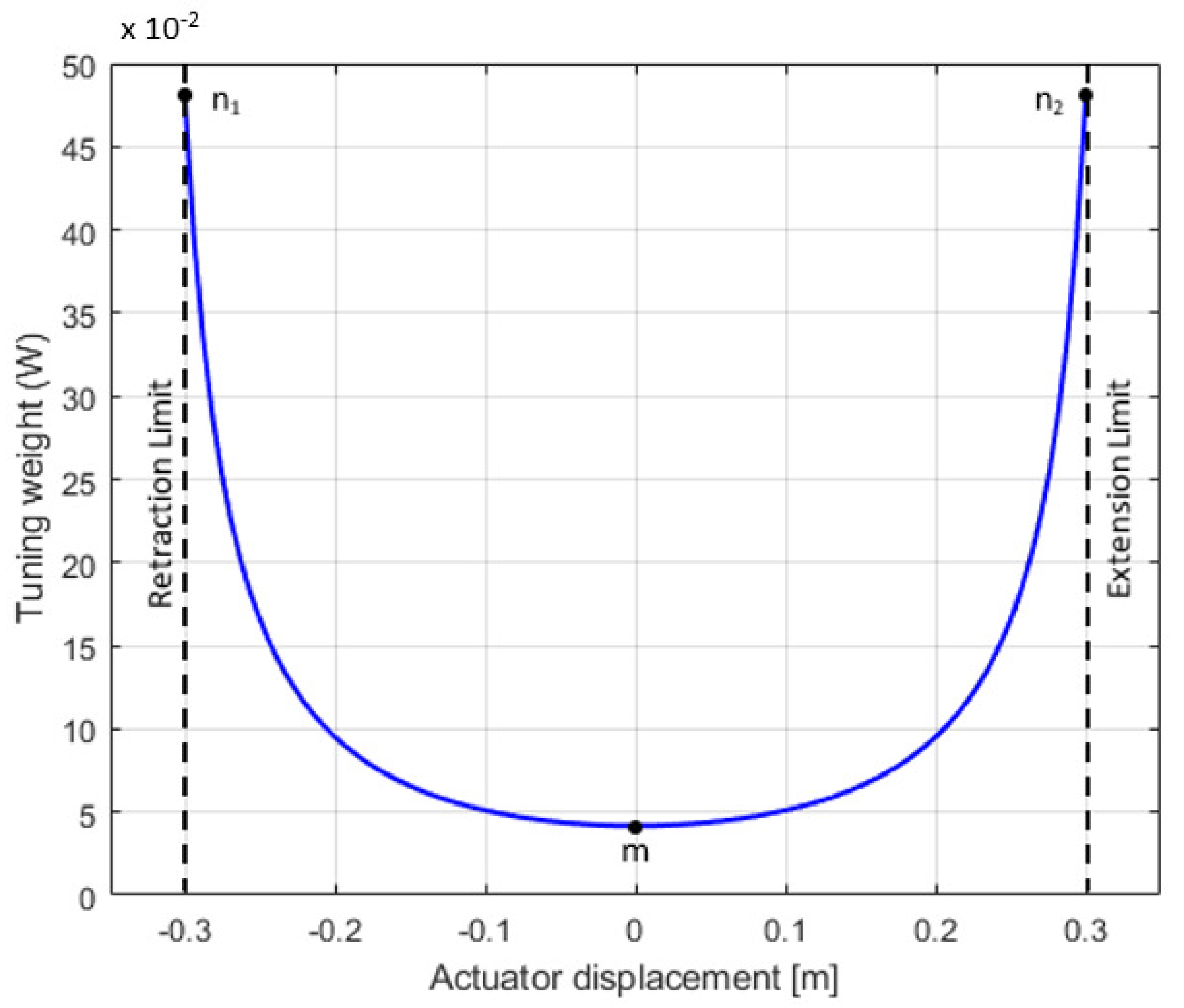
- Constraints on the actuator positions ().
4.3. Reference Generation
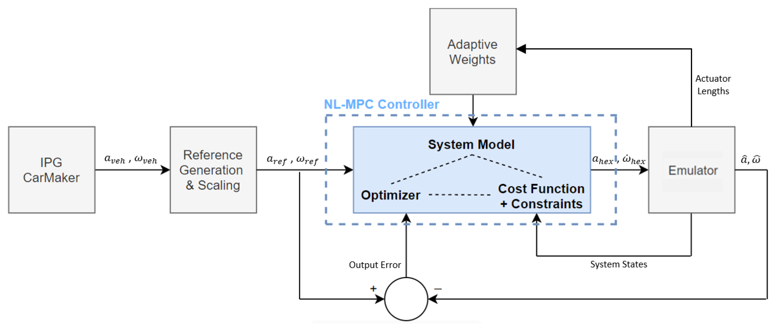
4.4. Adaptive Weight-Based Tuning
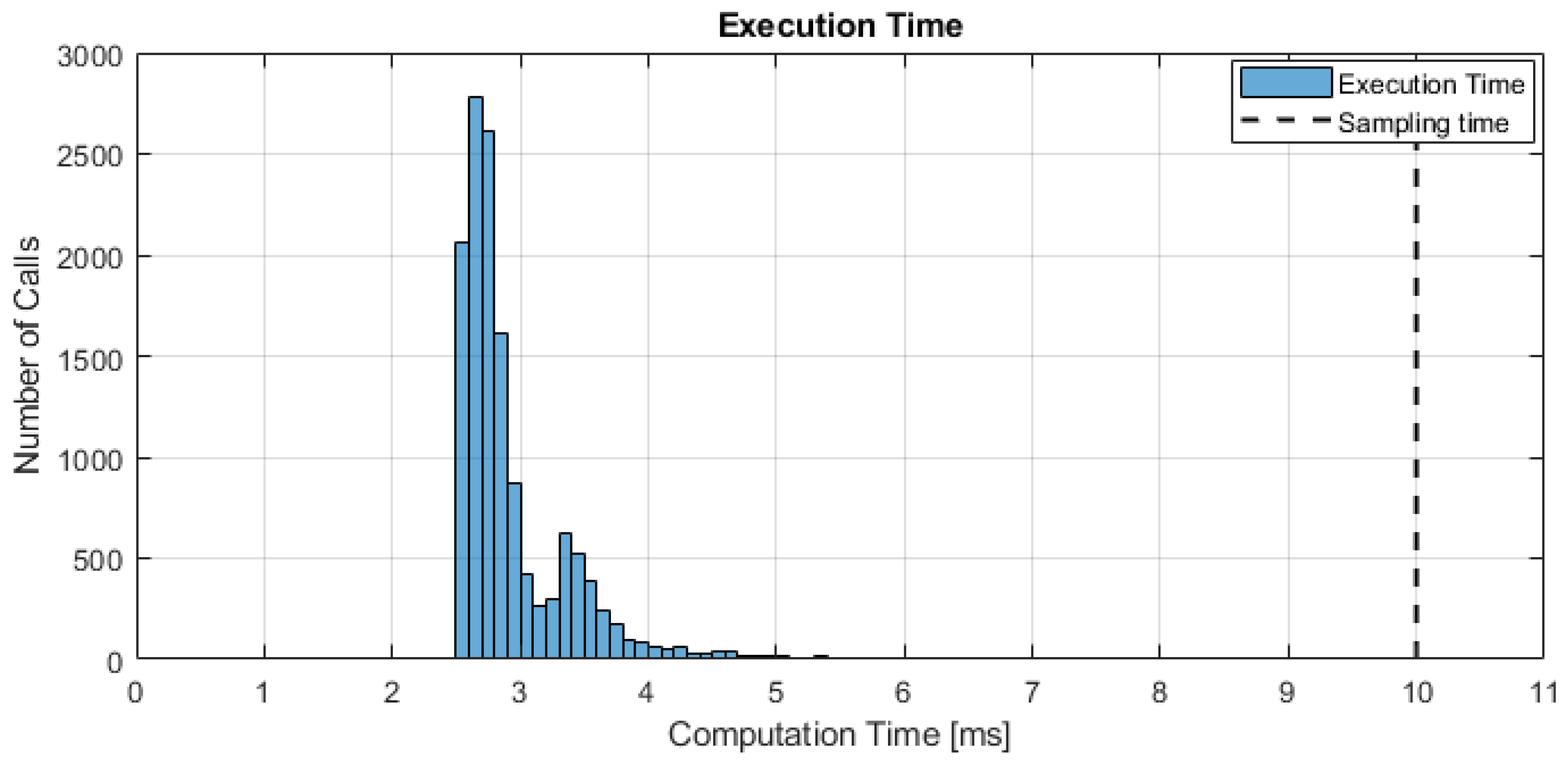
4.5. Optimization Problem
- Preparation step: The objective function is evaluated in the form of unknown state feedback . The original QP problem is formulated and condensed into a smaller and denser QP.
- Feedback step: The state feedback is substituted and the QP is solved to obtain the control input.
5. Performance Indicators
5.1. Indicators for Reference Tracking Performance
5.2. Indicators for Workspace Use
6. Results and Discussion
6.1. Simulation Setup
6.2. Simulation Results
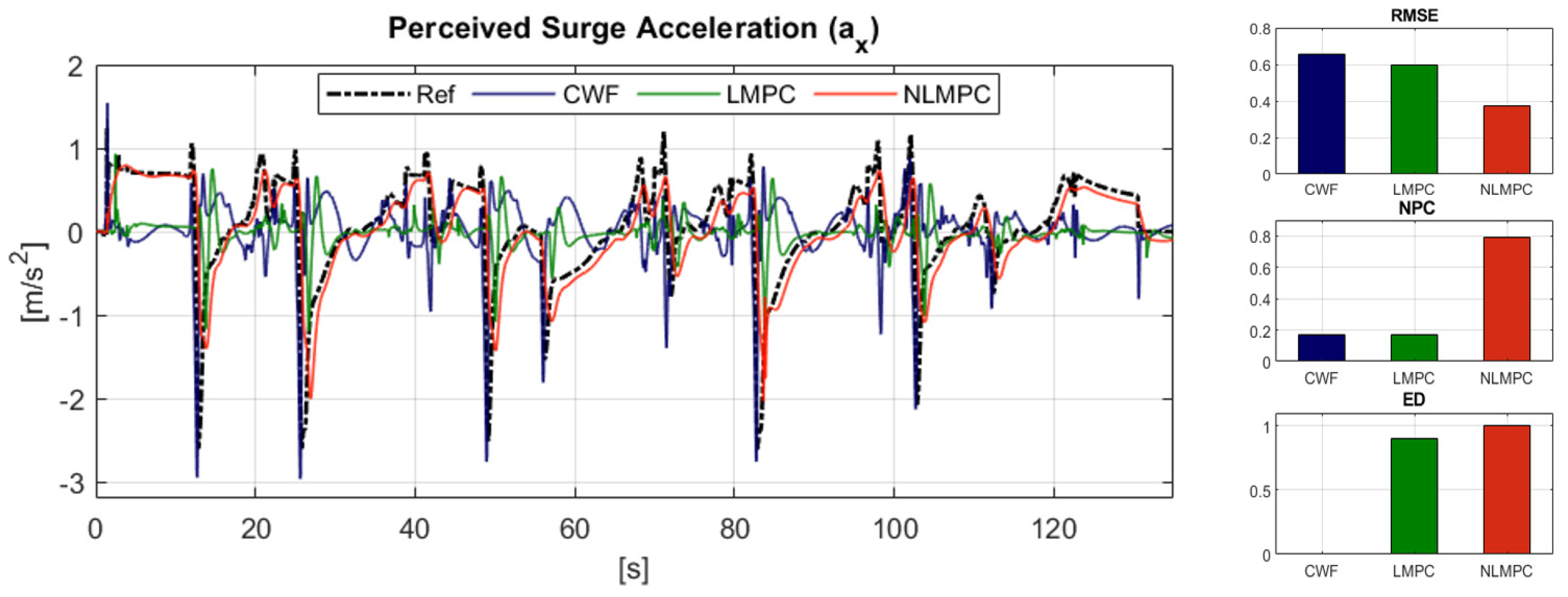
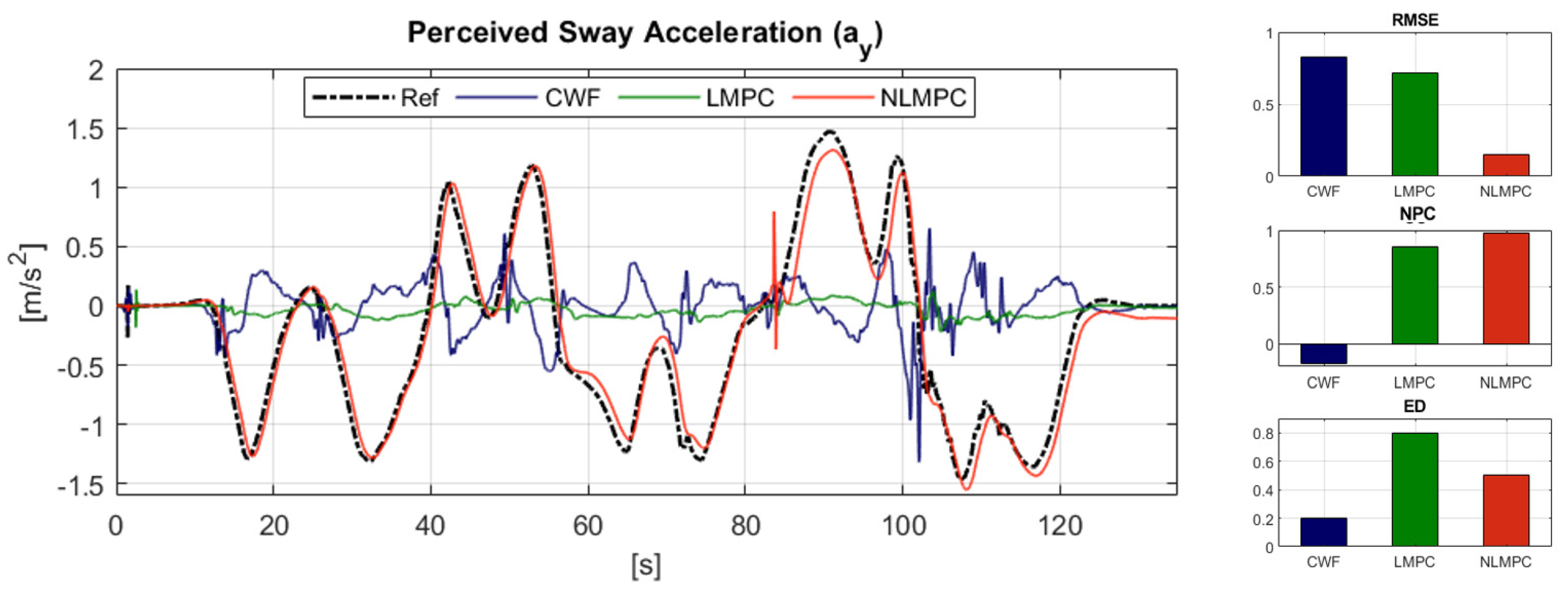
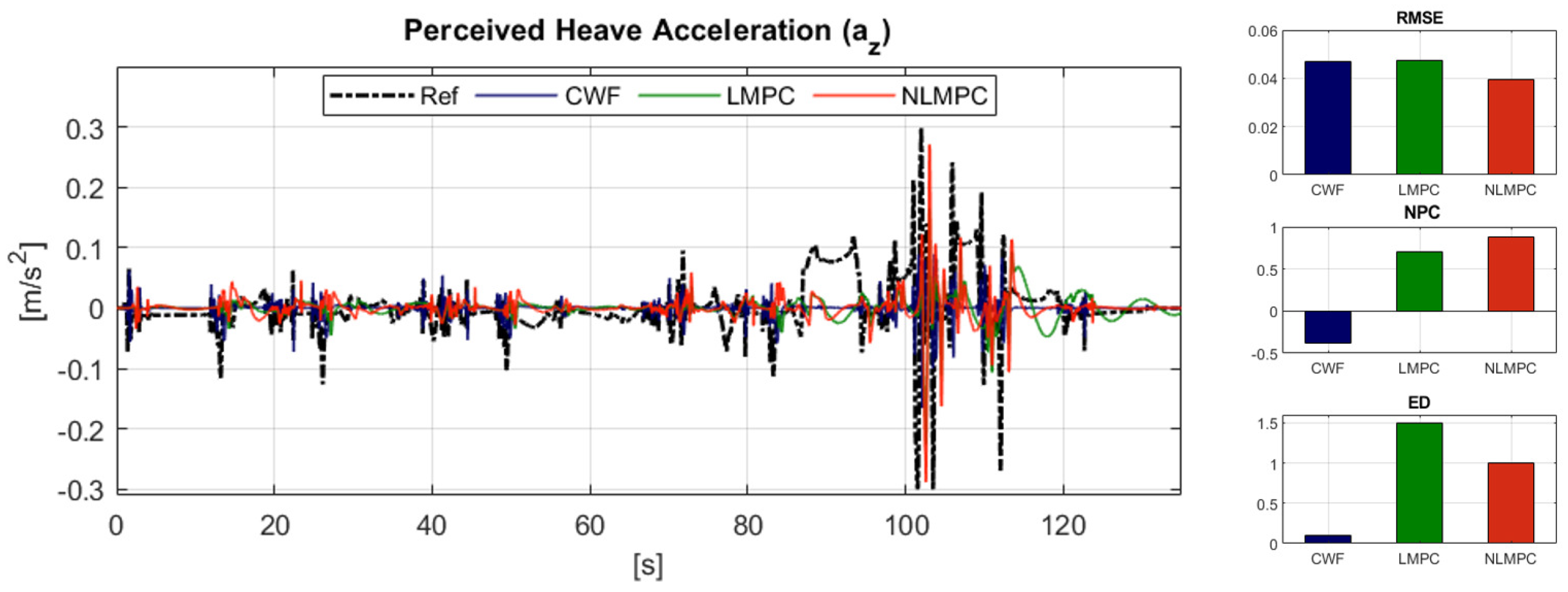
6.2.1. Reference Tracking Performance: Translational Acceleration
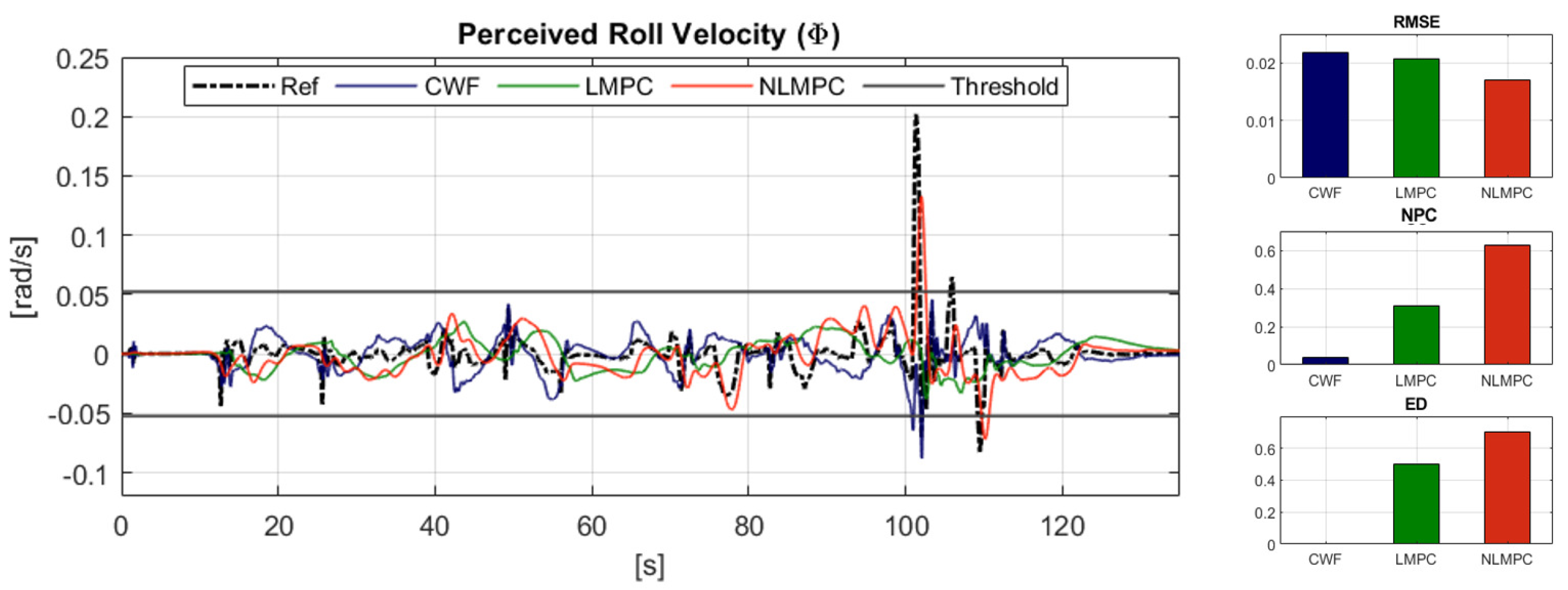
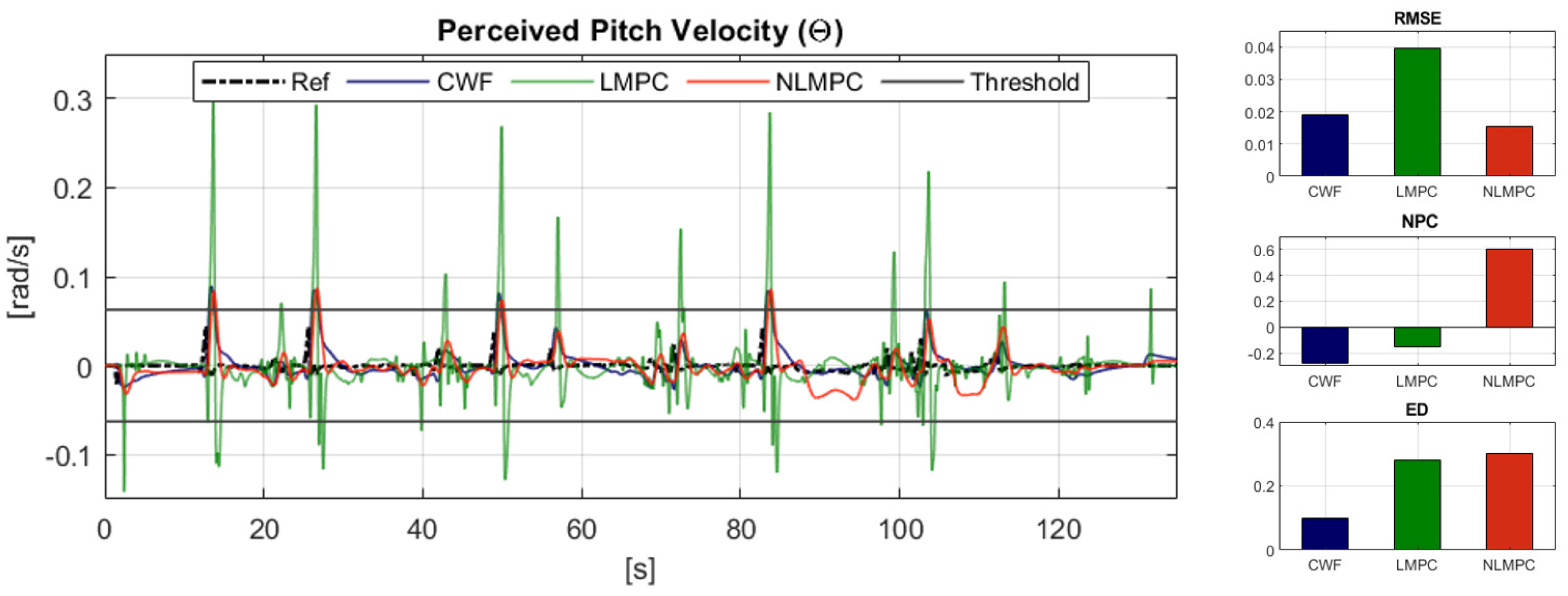
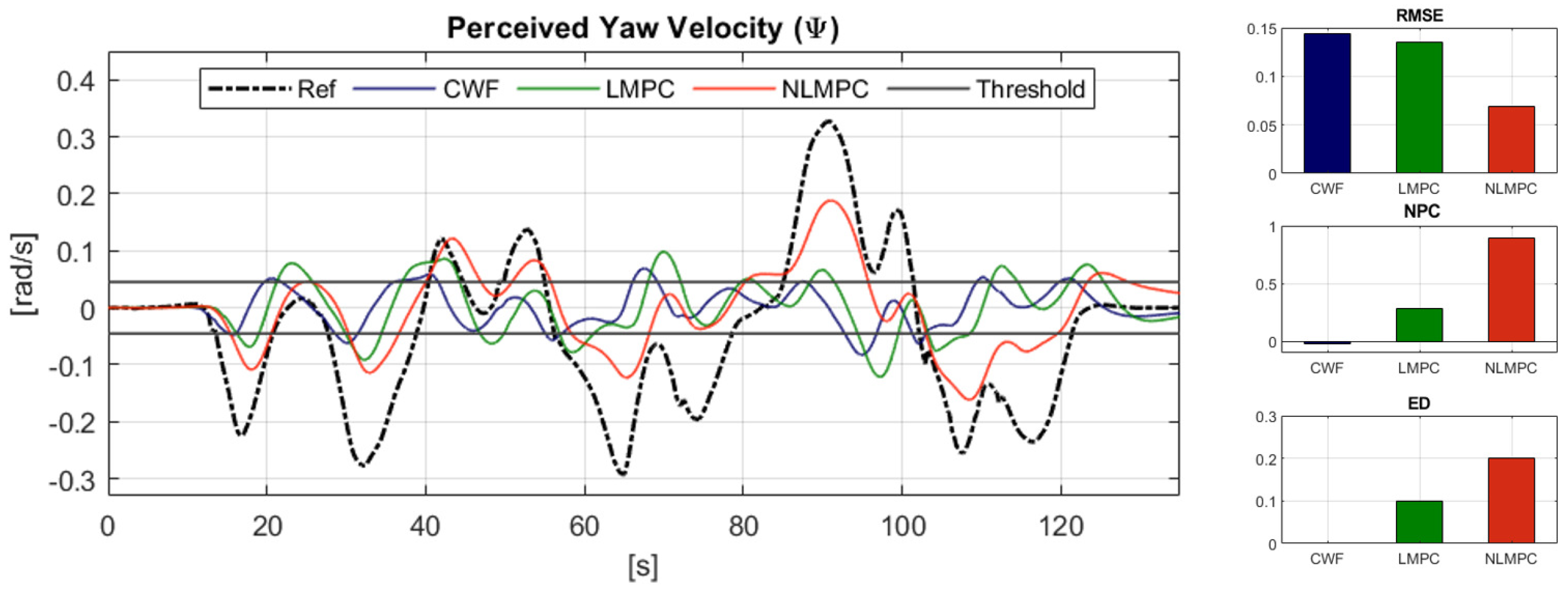
6.2.2. Reference Tracking Performance: Rotational Velocity
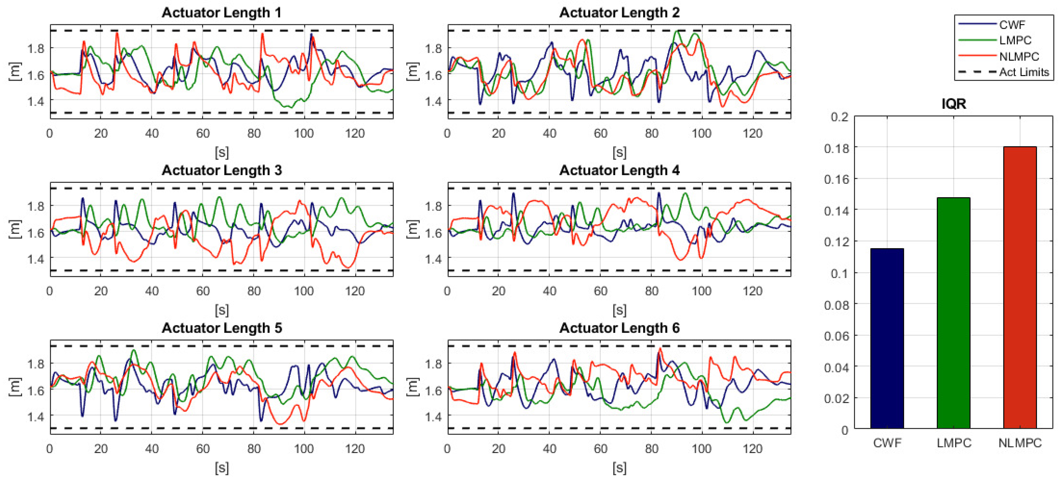
6.2.3. Workspace Use: Actuator displacement
7. Conclusions
Author Contributions
Funding
Conflicts of Interest
References
- De Winter, J.; van Leeuwen, P.M.; Happee, R. Advantages and disadvantages of driving simulators: A discussion. In Proceedings of the Measuring Behavior, Utrecht, The Netherlands, 28–31 August 2012; pp. 47–50. [Google Scholar]
- Shyrokau, B.; De Winter, J.; Stroosma, O.; Dijksterhuis, C.; Loof, J.; van Paassen, R.; Happee, R. The effect of steering-system linearity, simulator motion, and truck driving experience on steering of an articulated tractor-semitrailer combination. Appl. Ergon. 2018, 71, 17–28. [Google Scholar] [CrossRef]
- Nahon, M.; Reid, L. Simulator motion-drive algorithms—A designer’s perspective. J. Guid. Control. Dyn. 1990, 13, 356–362. [Google Scholar] [CrossRef]
- Sivan, R.; Ish-Shalom, J.; Huang, J. An optimal Control Approach to the Design of Moving Flight Simulators. IEEE Trans. Syst. Man Cybern. 1982, 12, 818–827. [Google Scholar] [CrossRef]
- Lamprecht, A.; Steffen, D.; Haecker, J.; Graichen, K. Comparision between a filter and an MPC-based MCA in an offline simulator study. In Proceedings of the Driving Simulation Conference and Exhibition, Strasbourg, France, 4–6 September 2019. [Google Scholar]
- Cleij, D.; Venrooij, J.; Pretto, P.; Katliar, M.; Bülthoff, H.H.; Steffen, D.; Hoffmeyer, F.W.; Schöner, H.-P. Comparison between filter- and optimization-based motion cueing algorithms for driving simulation. Transp. Res. Part Traffic Psychol. Behav. 2019, 61, 53–68. [Google Scholar] [CrossRef]
- Cleij, D.; Pool, D.M.; Mulder, M.; Bülthoff, H.H. Optimizing an Optimization-Based MCA using Perceived Motion Incongruence Models. In Proceedings of the 19th Driving Simulation and Virtual Reality Conference, Antibes, France, 9–11 September 2020. [Google Scholar]
- Van der Ploeg, J.R.; Cleij, D.; Pool, D.M.; Mulder, M.; Bülthoff, H.H. Sensitivity Analysis of an MPC-based Motion Cueing Algorithm for a Curve Driving Scenario. In Proceedings of the 19th Driving Simulation and Virtual Reality Conference, Antibes, France, 9–11 September 2020. [Google Scholar]
- Baseggio, M.; Bruschetta, M.; Maran, F.; Beghi, A. An MPC approach to the design of motion cueing algorithms for driving simulators. In Proceedings of the 14th IEEE international conference on Intelligent Transportation Systems, Washington, DC, USA, 5–7 October 2011; pp. 692–697. [Google Scholar]
- Bruschetta, M.; Maran, F.; Beghi, A. A fast implementation of MPC based motion cueing algorithms for mid-size road vehicle motion simulators. Veh. Syst. Dyn. 2017, 51, 802–826. [Google Scholar] [CrossRef]
- Husty, M. An Algorithm for Solving the Direct Kinematics of General Stewart-Gough Platform. Mech. Mach. Theory 1996, 4, 365–380. [Google Scholar] [CrossRef]
- Garrett, N.; Best, M. Model predictive driving simulator motion cueing algorithm with actuator-based constraints. Veh. Syst. Dyn. 2013, 51, 1151–1172. [Google Scholar] [CrossRef][Green Version]
- Dagdelen, M.; Reymond, G.; Kemeny, A. Model-based predictive motion cueing strategy for vehicle driving simulators. Control. Eng. Pract. 2009, 17, 995–1003. [Google Scholar] [CrossRef]
- Fang, Z.; Kemeny, A. Motion cueing algorithms for a real-time automobile driving simulator. In Proceedings of the Driving Simulation Conference, Paris, France, 6–7 September 2012. [Google Scholar]
- Katliar, M.; Fischer, J.; Frison, G.; Diehl, M.; Teufel, H.; Bülthoff, H. Nonlinear Model Predictive Control of a Cable-Robot-Based Motion simulator. IFAC-PapersOnLine 2017, 50, 9833–9839. [Google Scholar] [CrossRef]
- Katliar, M.; Olivari, M.; Drop, F.; Nooij, S.; Diehl, M.; Bülthoff, H. Offline motion simulation framework: Optimizing motion simulator trajectories and parameters. Transp. Res. Part Traffic Psychol. Behav. 2019, 66, 29–46. [Google Scholar] [CrossRef]
- Gros, S.; Zanon, M.; Quirynen, R.; Bemporad, A.; Diehl, M. From linear to nonlinear MPC: Bridging the gap via the real-time iteration. Int. J. Control. 2020, 93, 62–80. [Google Scholar] [CrossRef]
- Fichter, E.F. A Stewart platform-based manipulator: General theory and practical construction. Int. J. Robot. Res. 1986, 5, 157–182. [Google Scholar] [CrossRef]
- Dasgupta, B.; Mruthyunjaya, T.S. The Stewart platform manipulator: A review. Mech. Mach. Theory 2000, 35, 15–40. [Google Scholar] [CrossRef]
- Stewart, D. A Platform with Six Degrees of Freedom. Proc. Inst. Mech. Eng. 1965, 180, 371–386. [Google Scholar] [CrossRef]
- Fernandez, C.; Goldberg, J. Physiology of peripheral neurons innervating otolith organs of the squirrel monkey. III. response dynamics. J. Neurophysiol. 1976, 39, 996–1008. [Google Scholar] [CrossRef] [PubMed]
- Mayne, R. A Systems Concept of the Vestibular Organs. In Vestibular System Part 2: Psychophysics, Applied Aspects and General Interpretations. Handbook of Sensory Physiology; Kornhuber, H.H., Ed.; Springer: Berlin/Heidelberg, Germany, 1974. [Google Scholar]
- Young, L.; Oman, C. Model for vestibular adaptation to horizontal rotation. J. Aerosp. Med. 1969, 40, 1076–1077. [Google Scholar]
- Grant, W.; Best, W. Otolith-organ mechanics: Lumped parameter model and dynamic response. Aviat. Space Environ. Med. 1987, 58, 970–976. [Google Scholar]
- Ormsby, C. Model of Human Dynamic Orientation. Ph.D. Thesis, Massachusetts Institute of Technology, Cambridge, MA, USA, 1974. [Google Scholar]
- Telban, R.J.; Cardullo, F.M. Motion Cueing Algorithm Development: Human-Centered Linear and Nonlinear Approaches. NASA Tech Report CR-2005-213747. 2005. Available online: https://ntrs.nasa.gov/archive/nasa/casi.ntrs.nasa.gov/20050180246.pdf (accessed on 11 November 2020).
- Harib, K.; Srinivasan, K. Kinematic and dynamic analysis of Stewart platform-based machine tool structures. Robotica 2003, 21, 541–554. [Google Scholar] [CrossRef]
- Bock, H.; Plitt, K. A multiple shooting algorithm for direct solution of optimal control problems. In Proceedings of the 9th IFAC World Congress, Budapest, Hungary, 2–6 July 1984; pp. 243–247. [Google Scholar]
- Vukov, M.; Domahidi, A.; Ferreau, H.; Morari, M.; Diehl, M. Auto-generated algorithms for nonlinear model predictive control on long and on short horizons. In Proceedings of the 52nd IEEE Conference on Decision and Control, Florence, Italy, 10–13 December 2013; pp. 5113–5118. [Google Scholar]
- Magni, L.; Nicolao, G.; Magnani, L.; Scattolini, R. A stabilizing model-based predictive control algorithm for nonlinear systems. Automatica 2001, 37, 1351–1362. [Google Scholar] [CrossRef]
- Mayne, D.; Rawlings, J.; Rao, C.; Scokaert, P. Constrained model predictive control: Stability and optimality. Automatica 2000, 789–814. [Google Scholar] [CrossRef]
- Abdelaal, M.; Franzle, M.; Hahn, A. Nonlinear Model Predictive Control for Tracking of Underactuated Vessels under Input Constraints. In Proceedings of the 2015 IEEE European Modelling Symposium, Madrid, Spain, 6–8 October 2015; pp. 313–318. [Google Scholar]
- Grune, L.; Pannek, J. Stability and Suboptimality Without Stabilizing Terminal Conditions. In Nonlinear Model Predictive Control: Theory and Algorithms; Springer: Cham, Switzerland, 2011. [Google Scholar]
- Reid, L.; Nahon, M. Flight Simulation Motion-Base Drive Algorithms: Part 1—Developing and Testing the Equations; UTIAS Report No. 296, CN ISSN0082-5255; Institute for Aerospace Studies, University of Toronto: Toronto, ON, Canada, 1985. [Google Scholar]
- Houska, B.; Ferreau, H.; Diehl, M. ACADO Toolkit—An Open Source Framework for Automatic Control and Dynamic Optimization. Optim. Control. Appl. Methods 2011, 32, 298–312. [Google Scholar] [CrossRef]
- qpOASES Homepage. Available online: http://www.qpoases.org (accessed on 11 November 2020).
- Casas, S.; Coma, I.; Riera, J.V.; Fernández, M. Motion-cueing algorithms: Characterization of users’ perception. Hum. Factors 2015, 57, 144–162. [Google Scholar] [CrossRef]
- Grottoli, M.; Cleij, D.; Pretto, P.; Lemmens, Y.; Happee, R.; Bülthoff, H.H. Objective evaluation of prediction strategies for optimization-based motion cueing. Simulation 2018, 95, 707–724. [Google Scholar] [CrossRef]
- Grácio, B.; van Paassen, M.; Mulder, M.; Wentink, M. Tuning of the lateral specific force gain based on human motion perception in the Desdemona simulator. In Proceedings of the AIAA Modeling and Simulation Technologies Conference, Toronto, ON, Canada, 2–5 August 2010. [Google Scholar]
- Veltena, M.C. Movement Simulator. U.S. Patent No. 8,996,179, 31 March 2015. [Google Scholar]
- Van Doornik, J.; Brems, W.; de Vries, E.; Uhlmann, R. Driving Simulator with High Platform Performance and Low Latency. ATZ Worldw. 2018, 120, 48–53. [Google Scholar] [CrossRef]


| Degree of Freedom | Threshold Value |
|---|---|
| Roll | 3.0 deg/s |
| Pitch | 3.6 deg/s |
| Yaw | 2.6 deg/s |
| Parameter | |||||||
| Weight |
| Motion | Excursion [m] | Velocity [m/s] | Acceleration [m/s2] |
|---|---|---|---|
| Surge x | −0.51…0.63 | ±0.81 | ±7.1 |
| Sway y | −0.51…0.51 | ±0.81 | ±7.1 |
| Heave z | −0.42…0.42 | ±0.61 | ±10.0 |
| Roll | ±24.3 | ±35.0 | ±260.0 |
| Pitch | −25.4…28.4 | ±38.0 | ±260.0 |
| Yaw | ±25.0 | ±41.0 | ±510.0 |
| Actuator | 1.297…1.937 | - | - |
Publisher’s Note: MDPI stays neutral with regard to jurisdictional claims in published maps and institutional affiliations. |
© 2020 by the authors. Licensee MDPI, Basel, Switzerland. This article is an open access article distributed under the terms and conditions of the Creative Commons Attribution (CC BY) license (http://creativecommons.org/licenses/by/4.0/).
Share and Cite
Khusro, Y.R.; Zheng, Y.; Grottoli, M.; Shyrokau, B. MPC-Based Motion-Cueing Algorithm for a 6-DOF Driving Simulator with Actuator Constraints. Vehicles 2020, 2, 625-647. https://doi.org/10.3390/vehicles2040036
Khusro YR, Zheng Y, Grottoli M, Shyrokau B. MPC-Based Motion-Cueing Algorithm for a 6-DOF Driving Simulator with Actuator Constraints. Vehicles. 2020; 2(4):625-647. https://doi.org/10.3390/vehicles2040036
Chicago/Turabian StyleKhusro, Yash Raj, Yanggu Zheng, Marco Grottoli, and Barys Shyrokau. 2020. "MPC-Based Motion-Cueing Algorithm for a 6-DOF Driving Simulator with Actuator Constraints" Vehicles 2, no. 4: 625-647. https://doi.org/10.3390/vehicles2040036
APA StyleKhusro, Y. R., Zheng, Y., Grottoli, M., & Shyrokau, B. (2020). MPC-Based Motion-Cueing Algorithm for a 6-DOF Driving Simulator with Actuator Constraints. Vehicles, 2(4), 625-647. https://doi.org/10.3390/vehicles2040036