Article

The Sensitivity in Consumption of Different Vehicle Drivetrain Concepts Under Varying Operating Conditions: A Simulative Data Driven Approach

1
Department of Mechanical Engineering, Institute for Mechatronic Systems in Mechanical Engineering, TU Darmstadt, Germany
2
Department of Mechanical and Aerospace Engineering, Politecnico di Torino, Italy
*
Author to whom correspondence should be addressed.
Vehicles 2019, 1(1), 69-87; https://doi.org/10.3390/vehicles1010005
Submission received: 26 October 2018 / Revised: 21 December 2018 / Accepted: 6 March 2019 / Published: 14 March 2019

Abstract

:
As an important aspect of today’s efforts to reduce greenhouse gas emissions, the energy demand of passenger cars is a subject of research. Different drivetrain concepts like plug-in hybrid electric vehicles (PHEV) and battery electric vehicles (BEV) are introduced into the market in addition to conventional internal combustion engine vehicles (ICEV) to address this issue. However, the consumption highly depends on individual usage profiles and external operating conditions, especially when considering secondary energy demands like heating, ventilation and air conditioning (HVAC). The approach presented in this work aims to estimate vehicle consumptions based on real world driving profiles and weather data under consideration of secondary demands. For this purpose, a primary and a secondary consumption model are developed that interact with each other to estimate realistic vehicle consumptions for different drivetrain concepts. The models are parametrized by referring to state of the art contributions and the results are made plausible by comparison to literature. The sensitivities of the consumptions are then analysed as a function of trip distance and ambient temperature to assess the influence of the operating conditions on the consumption. The results show that especially in the case of the BEV and PHEV, the trip distance and the ambient temperature are a first-order influencing factor on the total vehicle energy demand. Thus, it is not sufficient to evaluate new vehicle concepts solely on one-dimensional driving cycles to assess their energy demand. Instead, the external conditions must be taken into account for a proper assessment of the vehicle’s real world consumption.

1. Introduction

The choice of a drivetrain concept for individual mobility in the form of passenger vehicles is regarded as a key determining factor for increasing sustainability and achieving a reduction in greenhouse gas emissions. Today, official vehicle energy demands are based on the results of consumption assessment on standardized testing procedures [1]. However, these procedures do not depict the diversity of real life usage. Hence, instead of using a standardized testing procedure, the real usage profiles of vehicles and further influences on the vehicle consumption should be taken into consideration. Thereby, the real ecological impact of a vehicle concept will not only depend on the drivetrain technology itself but also on the individual or representative driving profile as well as other external influences like geographical elevation data and ambient temperature. This procedure entails an extension of the system boundary since additional aspects related to the vehicle consumption are being considered. While standardized legislative driving cycles may provide a reliable foundation for the automotive industry regarding legal regulations over long time periods, they are static and not able to adapt to the evolving usage behaviour and advanced aspects as new vehicle technologies arise.
In our approach, representative driving cycles are generated based on real life driving data. The cycles are stochastically synthesized and offer an agile tool to depict real life usage. For showing the relevance of our approach within this work, we examine the sensitivity of the actual vehicle energy demand in real life driving scenarios as a function of ambient temperature and trip distance. Both of these parameters are especially important for the estimation of auxiliary consumer demands like heating venting and air conditioning (HVAC) which are here referred to as secondary demands. While internal combustion engine vehicles (ICEVs), for instance, make use of the engine waste heat for heating the interior and use the mechanical power available at the crank shaft for the air conditioning compressor, BEVs need to provide the energy from the battery. For plug-in hybrid electric vehicles (PHEVs), the amount of available waste heat decreases with an increasing percentage of electrical driving. At the same time the possible amount of electrical driving also depends on the secondary demand, which is why this interaction has to be considered in the determination of the primary and secondary energy demand.
Within this article, our aim is to show the relevance of this approach by assessing the energy demand of different vehicle concepts as a function of trip distance and ambient temperature and analysing the consumption sensitivities for different drivetrain concepts. Thus, different driving cycles are synthesized for multiple trip distances that represent the underlying driving profile. For this purpose, a simulation environment is developed to calculate the primary energy demand for moving the vehicle as well as the secondary energy demand required for HVAC.

2. State of the Art

2.1. Vehicle Consumption Modelling

As state of the art, the energy consumption of a vehicle is defined as the energy used for moving it over a specific distance [2]. All forces acting on the vehicle in this domain have to be considered. It is therefore modelled as a non-conservative system with dissipative terms reflecting driving resistances. Numerous software packages are used in literature to estimate primary vehicle consumption, for instance IPG CarMakerTM [3,4], AVL-CruiseTM [3,4] or MATLAB/SimulinkTM [5,6]. Models based on the driving resistances can be either forwards facing or backwards facing. Forwards facing models use a driver model, for example a simple PID-Controller, to follow the given driving cycle by calculating a traction demand based on the error between the set velocity and actual velocity. Backwards facing models assume that the vehicle is following the given driving cycle at each time and thus only calculate the required traction demand for this without the need of a driver model. In Reference [2], the consumption calculation based on a backwards facing powertrain model is introduced. Velocity and acceleration data in time domain is used to calculate the requested tractive torque on the side shaft by considering air drag, rolling resistance, road slope and acceleration force. An operating strategy is used to decide on the torque and energy management for a specific operating point. The operating strategy determines gear choices and the power distribution to the traction machines and thus determines requested torques and speeds at the crank shaft of the internal combustion engine and the output shaft of the electric machines. Efficiency maps are used to evaluate the losses in the traction machines and hence estimate the energy consumption in the operating points.

2.2. Secondary Demand Model

As introduced in Reference [7], vehicle secondary demands comprise the energy demands that are not directly connected to the movement of the vehicle. Amongst others, these are the energies needed for comfort demands, the vehicle’s electric system, the engine fan and so forth. The largest percentage of secondary energy is required for comfort demands, namely HVAC [8]. The secondary demand is often estimated by means of a simplified thermodynamic model of the passenger cabin. In reference [9], the authors designed a Computer-Aided Engineering (CAE) tool to compute the heat load of a vehicle passenger compartment using a lumped system approach considering solar radiation, conductive/convective heat transfers and passengers heat and moisture load. In reference [10], the authors analysed different control strategies and range impacts for EV integrated thermal management systems, considering a range of ambient temperatures between −20 °C and +20 °C, in order to obtain a range improvement compared to a basic strategy. They found that the HVAC technologies such as Positive Temperature Coefficient (PTC) elements or Heat Pumps and their control strategies have a major impact on the overall secondary energy consumption. Through using the electric motor and electronics waste heat with a heat pump and a PTC element in a new control strategy they were able to improve the vehicle range significantly.

2.3. Studies Concerning Range/Consumption

The increasing interest towards a sustainable mobility, that can be seen in the increasing development effort of battery electric vehicles (BEVs) and PHEVs, raises a number of new problems which were formerly negligible in vehicles solely powered by an internal combustion engine (ICE). These issues consist mainly in the increase in secondary energy consumption and the resulting decrease in range under certain external conditions, due to the secondary demands. These are by definition all systems which are not used to move the car but that help in increasing the comfort of driver and passengers and in increasing safety. The most energy consuming amongst all the secondary demands is the HVAC system (Heating Ventilation and Air Conditioning system), with a variable energy demand according to the ambient temperature. Thus, the ambient temperature has a significant influence on the range of vehicles, especially in the case of BEVs. Recently, different approaches were carried out in order to address this problem: In reference [11], the authors explored the interactive effects of ambient temperature and vehicle auxiliary loads on electric vehicle energy consumption. They monitored 68 EVs in Aichi Prefecture, Japan and developed an energy consumption model depending on ambient temperature and observed a minimum in consumption in the range of 21.8–25.2 °C. In reference [12], the authors developed a simple time-domain EV energy model computing the energy consumption based on vehicle speed, acceleration and road slope. They compared different electric vehicles by quantifying the impact of auxiliary systems, including air conditioning and heating systems on the overall system energy demand. They observed a significant range reduction of up to 24% at low ambient temperatures. In reference [13], the authors studied the effect of regional temperature differences on BEV range and CO2 emissions through electric energy production in the U.S., considering battery efficiency and cabin climate control. They found that at low temperatures, electric cabin heating consumes significantly more power compared to cooling down the cabin at high temperatures. At low temperatures, batteries have a lower performance resulting in a range decrease of up to 36% in cold climates.

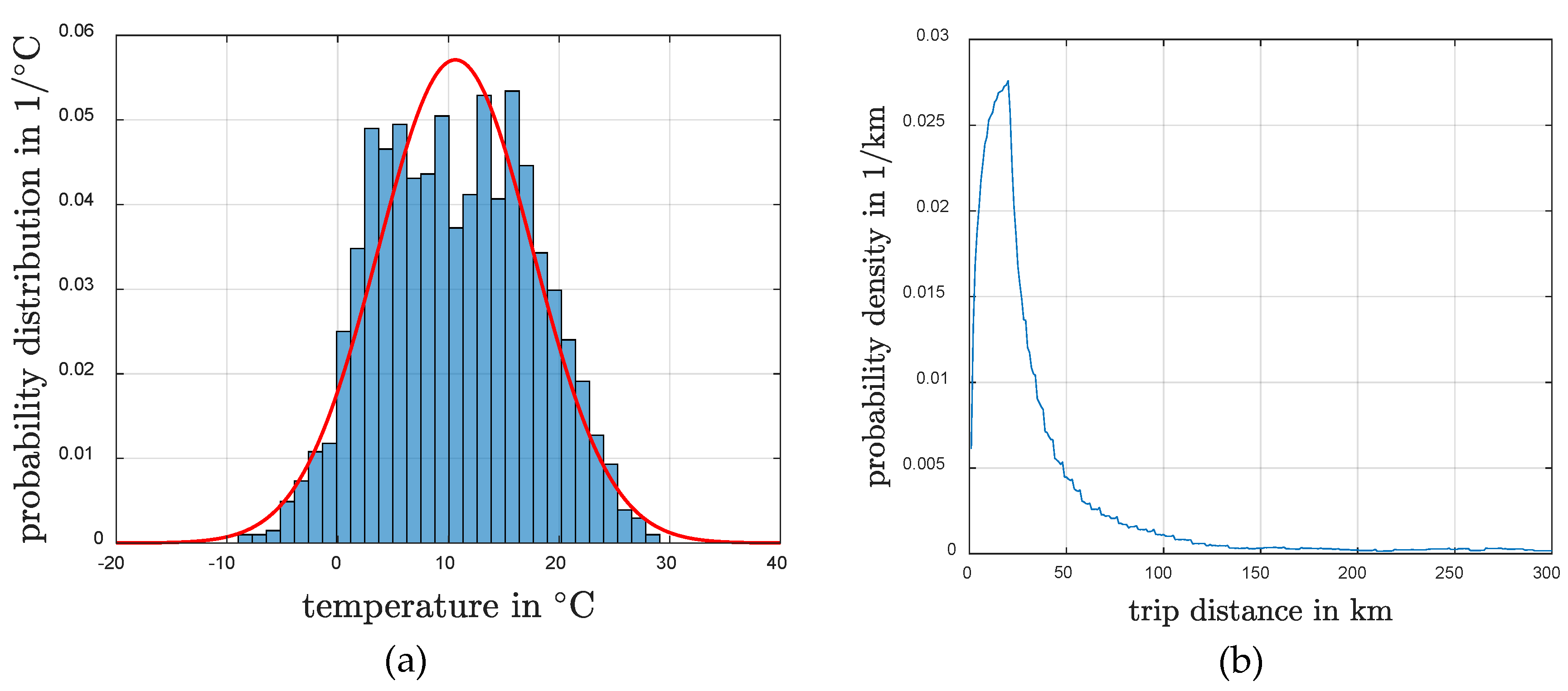
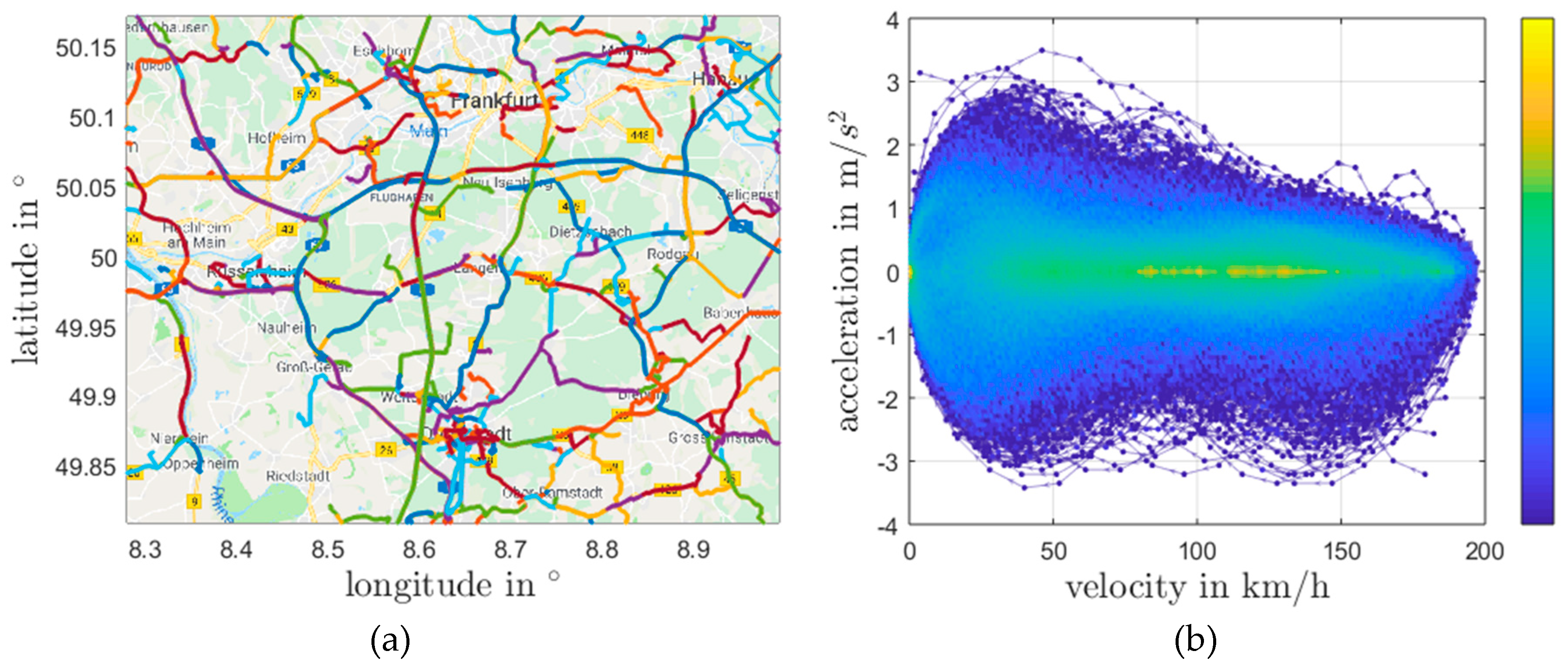
3. Data Basis for the Evaluation of Vehicle’s Consumption

As mentioned in the introduction, the scope of this work is a simulative analysis and comparison of different drivetrain concepts regarding the sensitivity of their consumption under varying external operating conditions. As Figure 1 shows, the operating conditions that are considered within this work, namely the external temperature and the driven trip distances vary significantly during the usage of a vehicle and their influence should be incorporated in the estimation of the overall energy demand. The vehicle’s energy demand can be classified into primary and secondary energy demands, as further discussed in Section 4. It is apparent that the primary energy demand strongly depends on the driving cycle that is used for the evaluation of the vehicle consumption. The secondary energy consumption though is also dependent on the driving cycle characteristics, because the heat transmission coefficients from cabin to exterior are a function of the vehicle’s velocity.
The main parameters which are going to be investigated in this work are the ambient temperature and the trip distance. Both are expected to have a major impact on the secondary energy demand for the HVAC of the cabin. The trip distance is of high relevance for the average consumption per distance since the cabin has to be heated from the ambient temperature to the desired cabin temperature for each single trip.
To compare the calculated energy demands as a function of trip distance, an equivalent driving cycle for each distance is necessary. Appending a reference cycle like the worldwide harmonized light duty test cycle (WLTC) multiple times to itself in order to obtain higher total distances limits the trip distance to integer multiples of the reference cycle’s distance, to avoid perturbation of the overall driving profile. Furthermore, scaling an existing driving cycle like the WLTC to different trip distances is not sufficient because this would lead to a different driving profiles which do not represent the underlying driving profile.
Instead, it is necessary to generate driving cycles with different trip distances that are representative for a given driving profile. Hence, the approach introduced in Reference [16] is applied to synthesize driving cycles of different trip-distances with the property that all cycles represent the respective overall driving profile. Details about the cycle synthesis algorithm are not a focus of this work but are presented in Reference [16].
To create a realistic real world driving profile, a database is built from GPS tracks provided by “OpenStreetMap” [17]. A large area around the cities of Darmstadt and Frankfurt in Germany was chosen as region of interest to represent a metropolitan area including urban, rural and highway driving. To enhance the quality of the generated database, all tracks are checked automatically and manually for physical plausibility and to guarantee that non-vehicle GPS tracks are omitted. During this process, only around 5% of the tracks were found to be of sufficient quality. Furthermore, a maximum velocity of 200 km/h is imposed to exclude extremely sporty driving from the investigation. An overview of the determined real world driving profile is given in Figure 2a,b. The driving profile is composed of 55 h of driving and a total travelled distance of around 16,000 km. The generated real world driving profile predominantly consists of idling and cruising phases. As expected, the highest accelerations occur at lower velocities while the maximum acceleration decreases with raising velocities.
As discussed before, it is necessary to synthesize driving cycles with different trip distances with the requirement that all cycles are representative of the overall profile seen in Figure 2b. To quantify how well the cycles represent the overall driving profile, different criteria are defined to compare the characteristics of the cycles to those of the overall profile. Concerning the state of the art, there is no consensus in literature which criteria should be used to guarantee a good estimation of the vehicle’s energy demand. In general, it is recommended to first define a criteria set θ containing multiple single criteria θ i to calculate the relative errors between the cycle and profile characteristics. Afterwards a mean error is determined that expresses the quality of a single cycle. In this study a criteria set θ of six single criteria θ are applied which are:
  • The mean velocity:
    θ 1   =   1 t end 0 t end v ( t ) d t
    where v is the vehicle velocity and t is the time.
  • The variance of the velocity signal:
    θ 2   =   1 t end 0 t end ( v ( t )     θ 1 ) 2 d t
  • The variance of the longitudinal acceleration:
    θ 3   =   1 t end 0 t end ( a ( t )     a ¯ ) 2 d t
    where a is the longitudinal acceleration of the vehicle.
  • The normalized energy demand for the air drag over the evaluation time:
    θ 4   =   1 s tot t τ acc t end v ( t ) 3 d t
    where s tot is the total traveled distance.
  • The normalized energy demand for the rolling resistance over the evaluation time:
    θ 5   =   1 s tot t τ acc t end v ( t )   d t
    where τ acc describes the time periods of cruising or acceleration situations.
  • The normalized energy demand for the acceleration resistance over the evaluation time:
    θ 6   =   1 s tot t τ acc t end a ( t )   v ( t )   m d t
Table 1 shows the exemplary calculation of the overall error based on the six single criteria θ i . Since the cycles are synthesized stochastically, the results vary according to a certain probability distribution and can thus vary in their quality. Therefore, for each defined distance, 10,000 cycles are synthesized, using the approach presented in Reference [16] and the best are chosen for further evaluation. This approach is shown in Figure 3, where the error distributions of all cycles for each trip distance are shown on the left and the cycles with the lowest overall error (regarding the criteria set θ) are shown on the right. Each error value was calculated according to the scheme shown in Table 1. The spacing of trip distance was chosen to be denser where the sensitivity of trip distance is expected to be higher. That is especially the case in the range of 50–100 km where the electrical range of the PHEV is expected. The best cycles for all distances have errors of less than 2 % compared to the overall fleet profile with the criteria set θ.
Using the best cycles enables the comparison of different vehicle’s consumptions as a function of trip distance since all the cycles are representative of the overall fleet profile. All the synthesized driving cycles impose almost equal demands on the vehicles concerning the velocity and acceleration distributions. Therefore, differences in the estimated consumption are almost exclusively caused by the required power of secondary demands that are dependent on ambient temperature and trip distance. The secondary consumption can likewise be calculated using a realistic velocity profile that directly influences the heat transfer coefficients of the cabin.

4. Vehicle Model

For investigating the influence of ambient temperature and trip length on the consumption of different vehicle concepts, valid models for primary and secondary energy demand are required. The goal of this section is to present the modelling of these demands. To analyse the sensitivity of consumption of different drivetrain concepts, an ICEV, a BEV and a PHEV in P2-configuration are chosen for the investigation and a simulation model is built to estimate the respective consumptions.

4.1. Primary Consumption Model

The primary energy demand modelling is based on a backwards model for the longitudinal dynamics with a time step size of Δt = 1 s that was built up in MATLABTM. The lateral and vertical dynamics of the vehicle are not considered, assuming that they have a neglectable effect on the vehicle consumption. Using a backwards facing model, as stated in Section 2.1, avoids the necessity of having a driver model. A driving resistance equation is used to calculate the required torque and rotational speed at the wheels for a given driving cycle and vehicle parameters. An efficiency map based modelling of the drivetrain is then applied to allow for an accurate estimation of the required energy demand. A brake specific fuel consumption (BSFC) map and an efficiency map taken from literature are used for the internal combustion engine (ICE) and electrical traction machine (EM), respectively, to model the losses in the machines as a function of torque and speed. The BSFC map is taken from ADVISOR model data [18], the efficiency map of the EM is based on measurements of a real machine [19,20]. For the multiple speed transmissions (ICEV and PHEV) and the single speed transmission (BEV), constant efficiencies are defined. The battery is likewise modelled with a constant charging and discharging efficiency. This approach yields a good trade-off between consumption estimation accuracy and computational effort.
An equivalent consumption minimization strategy (ECMS) is applied to determine the optimal operating points of traction machines for every time step [21]. The ECMS is applicable for all drivetrain concepts in the same way which further enhances the comparability of the results. Central part of the ECMS is the cost function J as shown in Equation (7) which quantifies an equivalent fuel mass flow rate of petrochemical and electrical energy and is minimized at each time step of the simulation [22]. For a chosen vector of valid discrete ICE torques, all possible combinations of ICE and EM power that satisfy the current traction demand of the driving cycle are calculated. Hence, J is a matrix whose components represent the respective costs for specific torque split and gear combinations. The operating point with the lowest cost is then chosen. The equivalent cost factor s is used to define a cost ratio between electrical energy and petrochemical energy. For the ICEV and BEV the cost function simplifies since they can only use one energy source. For the PHEV it is generally desired to maximize the use of electrical energy, which is done by tuning the equivalent cost factor s, such that the battery is depleted at the end of a trip. The energy demand of the secondary consumption model described in Section 4.2 is considered in the operating strategy by adding the consumption to the battery depletion. Therefore, the tuning of the equivalent cost factor s is dependent on the secondary consumption, thus an increasing secondary consumption results in less electrical energy available to move the car and a different operating strategy.
J   =   b e P ICE   +   s 1 L H V 1 η EM η batt P EM
where b e is the brake specific fuel consumption, P ICE is the current power of the combustion engine, L H V is the lower heating value of gasoline, η EM is the efficiency of the current operating point, η batt is the efficiency of the battery and P EM is the current power of the electrical machine.
The choice of the gear is the only degree of freedom for the ICEV to adjust the operating point of the engine in order to minimize consumption. In the case of the PHEV, gear choice and torque split between ICE and EM have to be determined which increases the computational effort. The torque split choice for the PHEV offers advanced functionality like load point shifting to potentially increase the overall efficiency. Regarding these load point shifts, boosting means applying a positive torque of both traction machines to be able to fulfil traction demands that are not possible for ICE only or to decrease the ICE torque to operate in an area of higher efficiency. Shifting on the other hand refers to a negative torque of the electrical machine in order to raise the torque of the ICE to an operating point of higher efficiency.
Typical sets of parameters are defined for each drivetrain concept, respectively. The main characteristics of the defined vehicles are summarized in Table 2. The total mass is the sum of the respective drivetrain and an identical chassis for all concepts. The drivetrain parameters are chosen such that the different concepts fulfil common design requirements, like a required starting torque and a maximum speed and the demands of the cycles regarding range and power. A BEV without a shiftable transmission typically needs a higher traction power compared to an ICEV to satisfy the design requirements. However, the chosen parameter sets are not optimal for the underlying driving profile and thus should only be considered as rough initial guesses to enable a qualitative comparison of the sensitivity regarding the operation conditions. In another contribution, a comparative optimization of drivetrain concepts was carried out to find optimal parameter sets for every concept and for different external parameters [23]. The use of such optimal drivetrain parameters enables a comparison of the absolute energy demand between the drivetrain concepts but this approach could not yet be included in the current work. Instead, the sensitivity of the energy demand of exemplary candidates for the considered drivetrain concepts is evaluated and compared.
Figure 4 shows the exemplary simulation results of the PHEV for one of the representative driving cycles. As stated before, the gear choice and torque split is performed by the ECMS. The operating strategy chooses the operating points to maximize the use of electrical energy which can be seen in the state of charge (SOC) curve. The SOC drops from 0.9 to 0.1, which have been defined as the maximum and minimum SOC, respectively. The operating points are chosen such that the ICE operates in the proximity of its peak efficiency. For longer trips, the cost of electrical energy is increased in order to distribute the same amount of electrical energy stored in the battery over a longer driving distance. In case of short trips, an almost solely electric operation is chosen and the ICE is only started if the EM alone is not sufficient for the driving power demand.
Additionally, the secondary energy demand, whose calculation is presented in the following section, affects the use of available battery capacity and is being considered by the operating strategy for the energy management and choice of operating points.

4.2. Secondary Consumption Model

The vehicle secondary consumption is the energy demand which is required in addition to moving the vehicle. As stated in Section 2.2, the main influence on secondary consumption is the energy for HVAC. In order to calculate its impact, a thermodynamic model of the vehicle cabin is derived. In a second step, depending on the examined vehicle concept and its HVAC technology, the electric and/or fuel energy demand can be calculated. Additionally, a constant energy demand is added for further auxiliary demands.
The thermodynamic model of the passenger cabin for estimating the secondary vehicle consumptions and thus for calculating the energy demand of the HVAC system is based on the approach introduced in Reference [7]. It incorporates the main mechanisms of heat transfer considering conduction, convection and solar radiation as well as the influence of humidity induced by the ambient air and the vehicle passengers. The model is developed in five degrees of freedom which are: cabin air temperature T cabin , dashboard temperature T dashboard , interiors temperature T interiors , doors temperature T doors and roof temperature T roof . The first law of thermodynamic leads to the following equations where the cabin represents the air mass inside the vehicle. Its temperature is the controlled variable of HVAC.
E . cabin = Q . dashboard + Q . window + Q . interiors + Q . doors + Q . roof + Q . driver + Q . passengers + H . in H . out
E . cabin = T . cabin ( m air c p , air + m water c p , water ) + m . water ( T cabin c p , water + Δ h v , 0 )
where E . cabin is the derivative of the cabin energy, Q . is the heat flux through the system borders, H . is the enthalpy through air entering and exiting the vehicle cabin, m air is the air mass inside the vehicle, c p is the specific heat capacity, m water is the water mass inside the cabin and Δ h v , 0 is the evaporation enthalpy of water.
The interiors comprise mainly the seats, which have a relatively high thermal capacity compared to the surrounding air. They are also the most relevant energy capacity when heating the car in colder conditions to the steady state set temperature.
T . interiors m interiors c p , interiors = Q . interiors
where m interiors is the mass of interiors and thus especially of the seats.
Solar radiation is absorbed in the dashboard which in turn exchanges heat convectively with the cabin air mass.
T . dashboard m dashboard c p , dashboard = Q . solar Q . dashboard
Q . solar = I radiation γ α A dash
where m dashboard is the mass of the dashboard, Q . solar is the heat flux through solar radiation, I radiation is the intensity, γ is the absorbance of the dashboard, α is the transmittance of the windshield and A dash is the area of the dashboard.
The doors, the roof and the windows of the vehicle are the interface to the environment and are represented as thermal masses which exchange heat through convection with the external air as well as the cabin air mass.
T . doors m doors c p , doors = Q . doors , ext Q . doors , int
T . roof m roof c p , roof = Q . roof , ext Q . roof , int
where m doors is the mass of the doors, m roof is the mass of the roof and Q . are the respective heat fluxes.
The vehicle passengers are another influencing factor and are modelled as a source of heat and water mass. The human metabolic rate and the number of passengers lead to a constant heat flow which is emitted into the cabin air.
Q . passenger = n λ A body
m . water , passenger = 8.3 n · 10 6 kg s
where n is the number of passengers inside the vehicle, λ is the human metabolic rate and A body is the area of the human body.
Additionally, the water mass induced by the passengers is calculated as a constant flow rate such that the total water mass inside the cabin can be calculated with respect to the recirculating air, the fresh air from outside and the dehumidification by the air conditioning system. It is characterized by a constant dehumidification factor and is activated in case the sultry limit of 13 g water kg dry   air   is exceeded [25]. The limit is set as state of the art and is to improve passenger comfort as well as road safety through preventing a misted windscreen.
m . water = ( m . circair m . air ) X cabin + m . freshair X ext + m . water , passenger β m . air X cabin
X cabin   =   m water m air
where β is the dehumidification factor, X is the water loading, m . circair is rate of the recirculating air mass, m . freshair is the rate of fresh air mass entering the vehicle, m . air is the rate of the vehicle air mass and m water is the total water mass inside the vehicle cabin.
The cabin temperature can be set by the HVAC system by controlling the enthalpy flow into the system.
m . in = m . circair ( T cabin c p , air + X cabin ( T cabin c p , steam + Δ h v , 0 ) ) + m . freshair h freshair + Q . HVAC
H . out = m . air ( T cabin c p , air + X cabin ( T cabin c p , steam + Δ h v , 0 ) )
The enthalpy entering the system is defined as the amount of circulating and fresh air and their corresponding enthalpies. The cabin temperature of the vehicle is controlled by setting up a positive or negative heat flow Q . HVAC . At the same time the corresponding amount of air leaves the cabin which is considered in H . out . With the help of these formulations the main thermodynamic effects can be observed through simulation.
So far, a thermodynamic model was derived to estimate the energy demand for HVAC. Additionally, to compute the influence of secondary demands on the vehicle energy consumption, the underlying technology for HVAC needs to be considered. In this work, a BEV, a PHEV and an ICEV are examined.
Concerning a BEV, the state-of-the-art system for HVAC is a PTC element for heating and a conventional air conditioning for cooling. A PTC Element is a simple resistor that converts electric energy directly into thermal energy. Some BEVs are also equipped with additional heat pumps which offer a better performance by using the enthalpy of ambient air. However, these systems are not capable of heating in harsh conditions at very low temperatures and are therefore not considered in our work.
A PHEV needs to be equipped with multiple systems. In case of a running combustion engine, the waste heat can be used by a heat changer for heating the passenger cabin. In case of purely electric driving, an additional PTC element needs to be used to heat the cabin. The air conditioning does not depend on the operating mode and is thus realized with a conventional system.
Due to the abundance of waste heat, the ICEV does not need to generate heat flow through electric energy. With the help of a heat exchanger, the engine waste heat is used to provide sufficient heating power for meeting cabin temperature requirements. Upper class vehicles use PTC elements for providing a dynamic heating behaviour in order to increase passenger comfort. This results in an increased energy demand because of the required electrical energy that is generated by the alternator. However, this supplementary system is only present in a minority of vehicles and only induces a negligible part of the energy demand needed for HVAC. Therefore, these systems are not considered within this work. Table 3 summarizes the distribution of HVAC technology for different vehicle concepts.
In this section, a description was given on how the secondary energy demand can be derived from vehicle thermodynamic equations. Based on the demand and the underlying HVAC technology which is dependent on the respective vehicle concept, the energy consumption of secondary demands can be calculated by using different constant efficiency values.
It should be stated that the primary and secondary energy consumption calculation are carried out simultaneously and interact with each other. For instance, in case of a PHEV, the secondary energy consumption depends on the operating strategy since different technologies are used when driving purely electric or with the combustion engine turned on. Thus, a higher demand in electric energy for heating results in a reduced electric range which influences the primary energy consumption because the operating strategy is different.

5. Results

In this section, the results of the computed consumption of different drivetrains concepts as a function of trip distance and ambient temperature are presented. As discussed in Section 3, a cycle synthesis method was applied to generate cycles for all trip distances with the requirement that they represent the characteristics of the overall driving profile. This enables the calculation of the primary and secondary energy demands using realistic velocity traces and ensure a representative driving style at the same time. Therefore, the differences in consumption only result from the parameters of interest and not the different driving cycles.

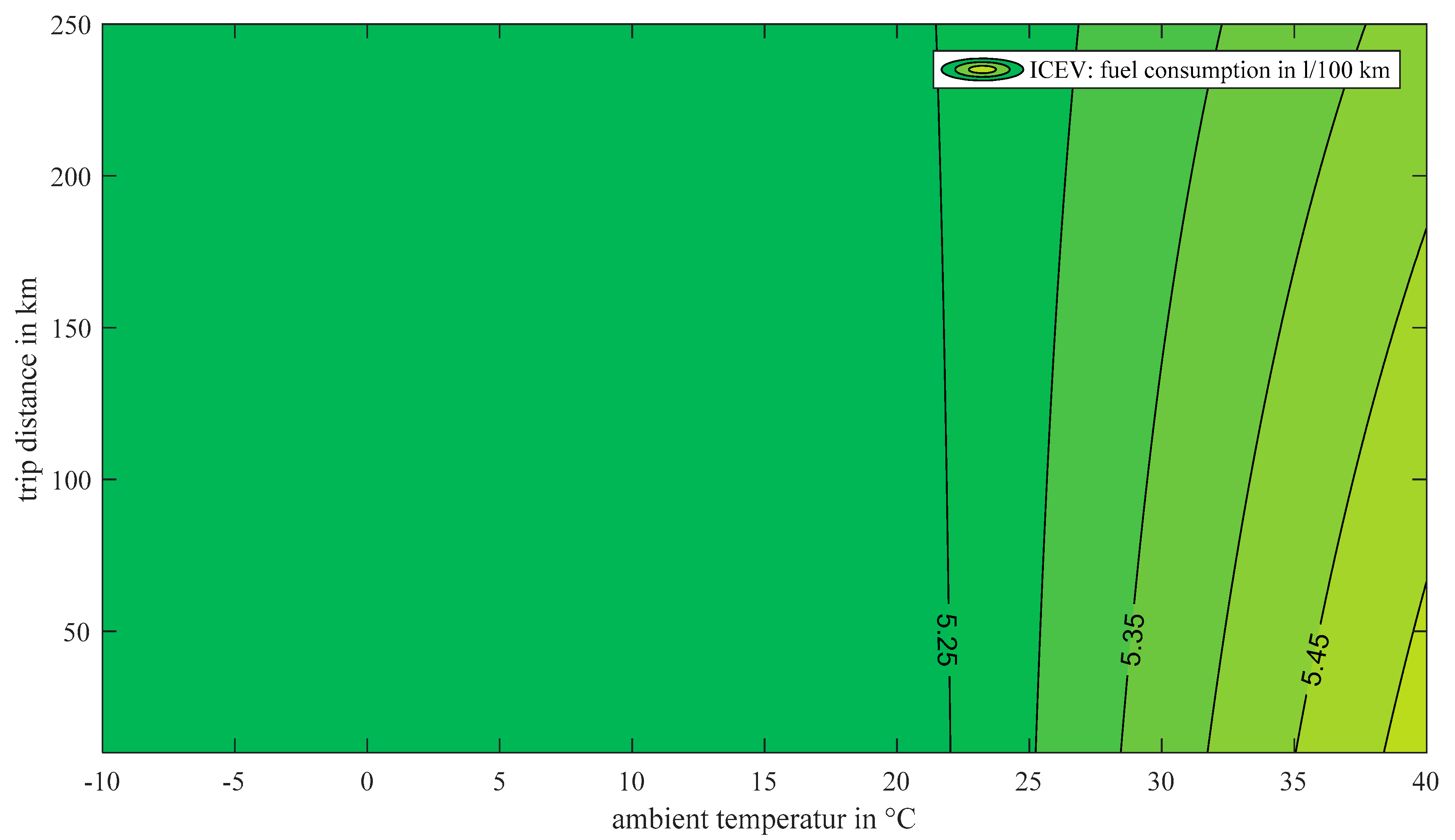
5.1. Internal Combustion Engine Vehicle

The results of the determined fuel consumption of the ICEV in l/100 km is shown in Figure 5. The graph is divided into two regions, above and below the desired internal cabin temperature of 21 °C. In the region below the desired cabin temperature, the consumption is very insensitive to trip distance and ambient temperature. There is normally more enough waste heat from the engine usable for climate control purposes even in very cold environments. Due to the fact that the waste heat is always available for heating and can been drawn with no influence on the fuel consumption there is a very low dependency in trip distance. Therefore, the consumption of an ICEV is very insensitive to ambient temperatures of up to 21 °C, which, for the given climate in Germany, are the most relevant operating conditions as shown in Figure 1. Regarding higher ambient temperatures, the consumption increases slightly because of the additional energy demand for cooling the vehicle cabin. The impact is moderate though due to the relatively high efficiency of the air conditioning system. Additionally, short trip distances lead to increased consumptions compared to longer trips because the time period necessary for cooling the vehicle in relation to the total trip length is higher, leading to a higher mean power demand for the secondary demand. The maximum absolute and relative differences in determined consumptions for the analysed range of trip distance and ambient temperature are 0.3 l/100 km and 5.5%, respectively.

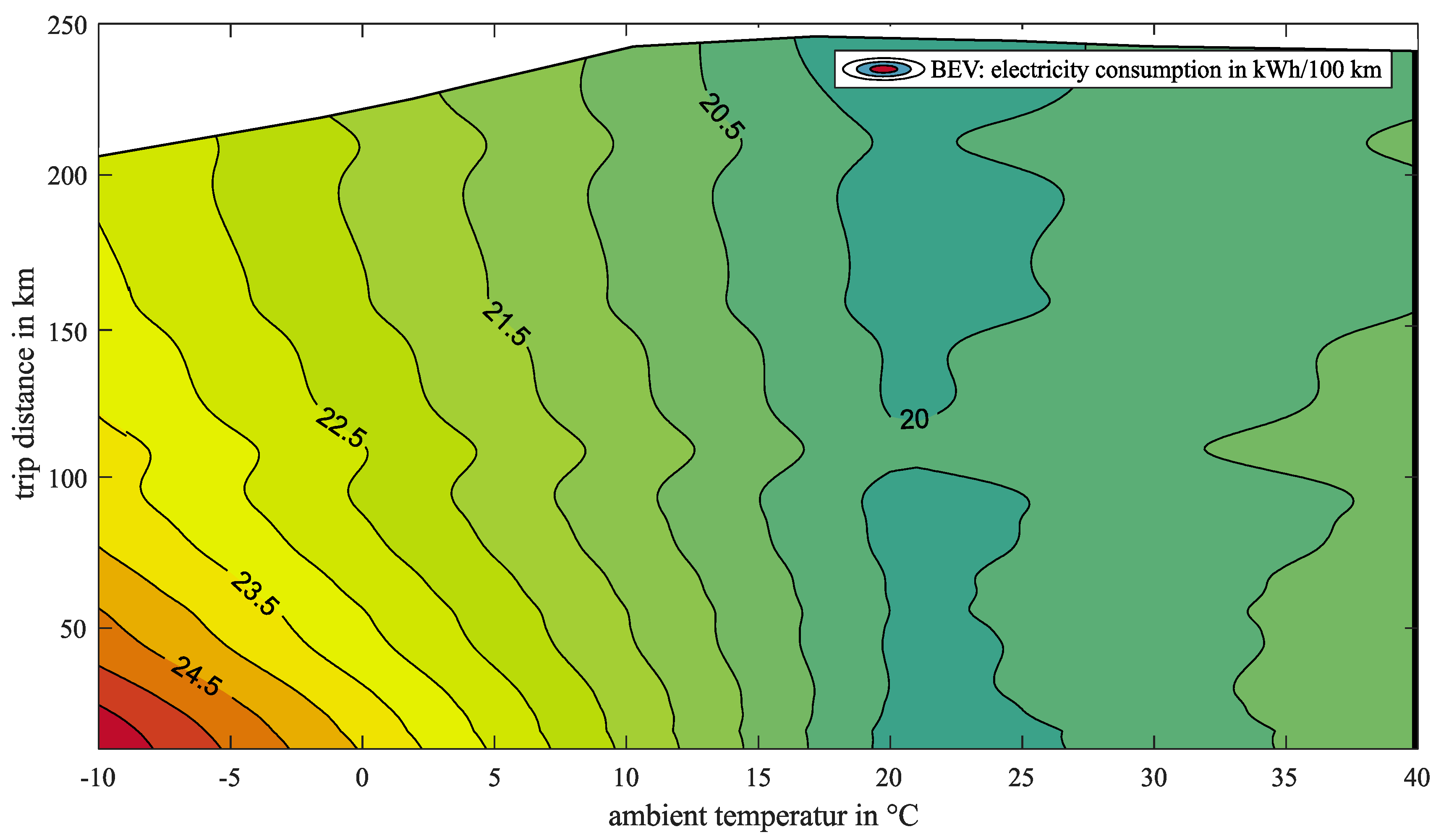
5.2. Battery Electric Vehicle

Similarly, to the analysis of the ICEV, the consumption of the BEV in kWh/100 km is determined for all trip distances and temperatures. The results are shown in Figure 6. Compared to the ICEV, the sensitivity in consumption is much higher in the whole analysed area of trip distance and ambient temperature. First of all, the temperature has a strong influence in all operating regions. The gradient of consumption towards lower ambient temperatures than the cabin’s set temperature is higher than towards increased ambient temperatures. The additional energy demand is especially affecting the consumption in heating scenarios with cold external conditions and is less relevant for warm conditions where the cabin has to be cooled down. This is due to the PTC elements that have to provide the whole heating power since no engine waste heat is available. For cooling, the air conditioning system is used resulting in a less significant additional energy demand at higher ambient temperatures. Regarding the influence of the trip distance, a much higher variation in consumption can be seen in comparison to the results of the ICEV especially for cold ambient temperatures. When the vehicle has to be heated to the desired cabin temperature from cold starting conditions within a very short trip, a high amount of power is required within a short time span leading to an increase in consumption. For longer trips, the influence of the secondary energy demand on the consumption is lower since after heating up the cabin, the power required to maintain the stationary conditions is lower for the remaining part of the trip.
The maximum difference in determined consumption is 5.85 kWh/100 km with a relative variation of 22.7%. When compared to the results of the ICEV, a much higher variation in energy demand as a function of the operating conditions occurs.
Note that the defined battery capacity is not sufficient to finish all trips, which is illustrated by the blank region in Figure 6. That is because at higher consumptions the maximum possible vehicle range is reduced.

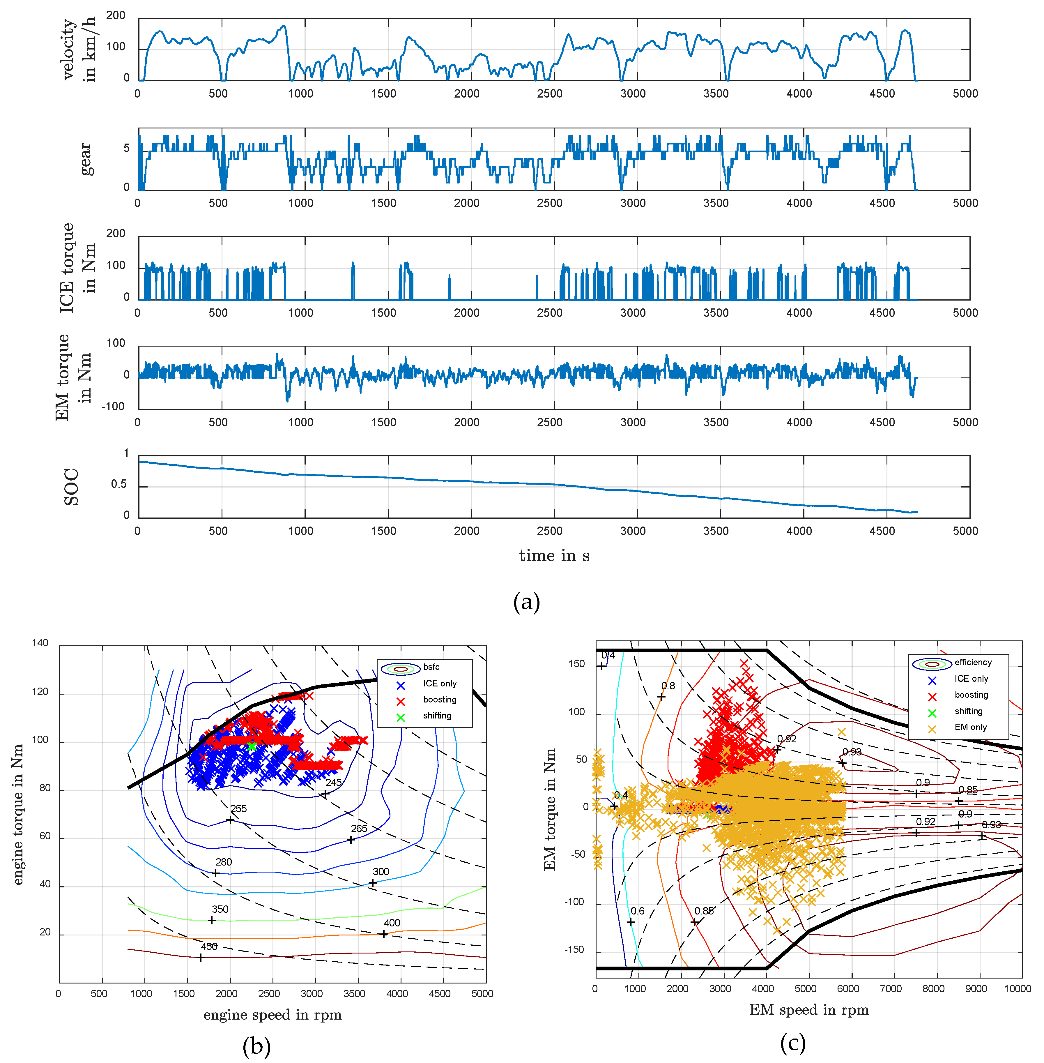
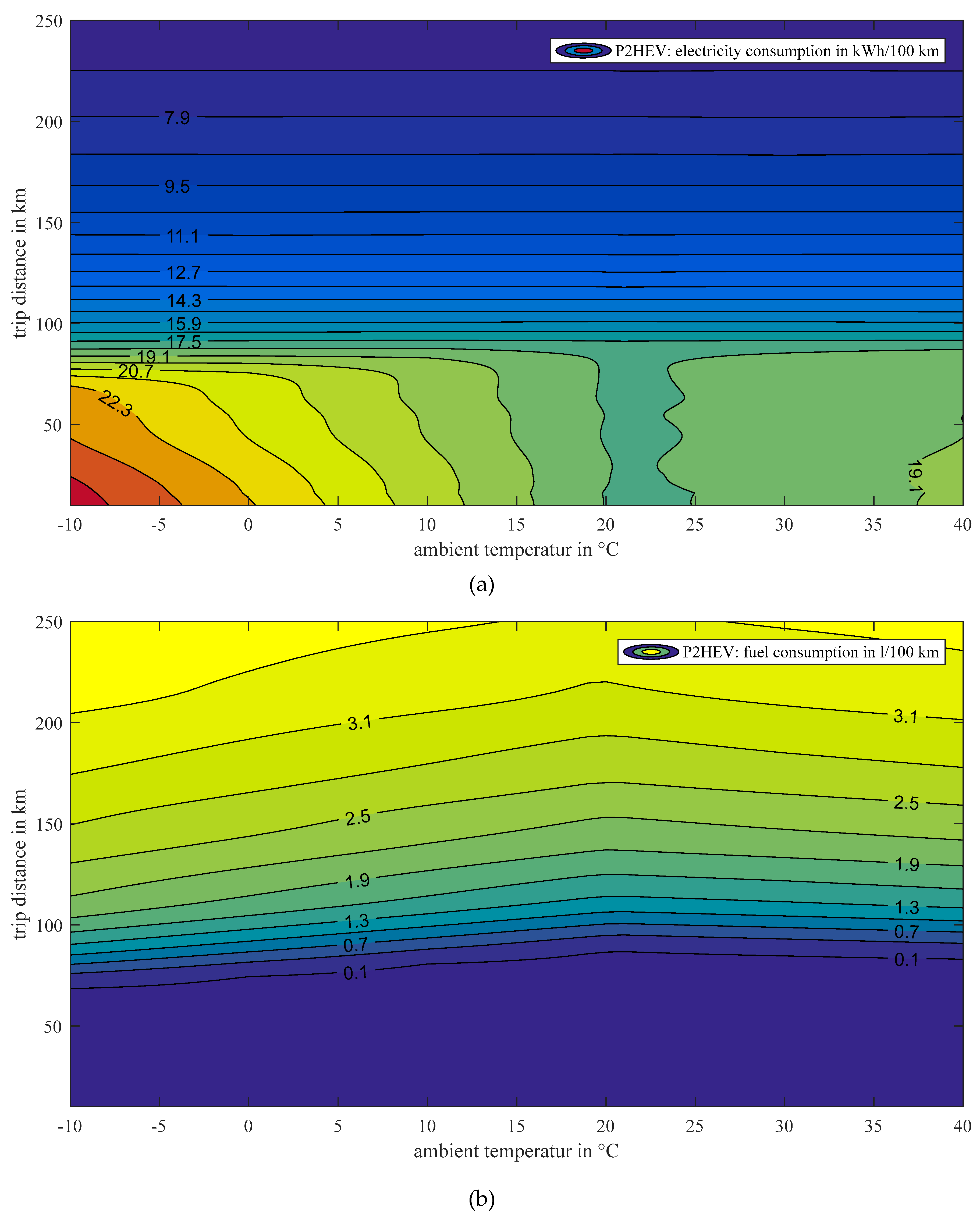
5.3. Plug-In Hybrid Electric Vehicle

In case of the PHEV, the consumption maps for both electric energy and fuel are calculated. As described above, the operating strategy does not operate in charge sustaining mode but tries to fully deplete the battery for each trip distance. Therefore, the vehicle is driving almost purely electrical at low trip distances. The results, which are shown in Figure 7, show a complex behaviour that is decomposed in the following. It is assumed that the PHEV starts each trip with a fully charged battery and ends with a depleted battery for trip distances above the electric range.
The electric consumption map can be divided into two regions, separated by the electric range of the vehicle. The electric range as a function of ambient temperature can approximately be derived from the fuel consumption plot as it is located close to the first contour line where the fuel consumption is greater than zero. In the region below the electric range of the vehicle, the PHEV can drive almost purely electric. Therefore, the fuel consumption is nearly zero. Very small values can occur though, since it is possible that the vehicle needs the ICE and EM power at the same time to fulfil a requested driving manoeuvre. In general, in the region below the electric range, the PHEV has a similar characteristic to the BEV. High and low ambient temperatures increase the electric consumption for the climate control of the cabin, with colder ambient temperatures being more energy intensive. Therefore, as for the BEV, the electric range is dependent on the ambient temperature due to the secondary demands. There is also a high sensitivity to trip distance in this region, since the vehicle has to be heated to stationary conditions with a high demand in power for HVAC. Hence, the energy required to heat the cabin accounts for a greater percentage of the total energy demand. Thus, the highest electrical consumption occurs at low trip distances and low ambient temperatures.
The second region above the electric range shows a completely different sensitivity to ambient temperature and trip distance. The electrical consumption is now independent from ambient temperatures because the battery is always fully depleted during each trip and all ambient temperatures. This means that the electric consumption can be directly derived from the quotient of available battery capacity and trip distance, thus forming a hyperbole function of trip distance. Higher overall energy demand is still required for low temperatures due to secondary demands, which results in an increase in fuel consumption.
In general, the operating strategy can decide on factors like the percentage of purely electric driving, boosting or load point shifting. The chosen operating strategy and the assumption that the battery, if possible, is always fully depleted after each trip, has a major influence on the results. This assumption leads to the abrupt change in sensitivity when exceeding the electric range. Additionally, higher trip distances lead to a higher percentage of the ICE being turned on. Therefore, more waste heat is available that can be used to heat the cabin. The figure shows that colder ambient temperatures are more energy intensive than warmer conditions for medium trip distances (around 100–150 km), since the electric driving percentage is still high, resulting in less available waste heat. For longer trip distances, the electric driving percentage diminishes and the vehicle can use the additional waste heat from the ICE in colder temperatures. Therefore, at around 250 km, the dependency of the energy demand on ambient temperature decreases. When even longer trip distances are considered, the PHEV increasingly approaches the characteristics of the ICEV with very robust consumption behaviour in colder environments. The determined electrical and fuel consumption values are calculated under the assumptions that the vehicles start with a maximum state of charge and that the operating strategy tries to maximize the electrical driving percentage. It can therefore be considered as an optimal result in terms of the potential in CO2 reduction having the increasing percentage of renewable energies on the energy mix in mind.
The results show that the consumption characteristic of a PHEV is strongly dependent on the usage profile. According to the typical distribution of trip distances, shown in Figure 1b, short trips are the most relevant, hence the PHEV in reality is often operated with a very high electric driving percentage, thus a high dependency of its consumption on ambient temperature and trip distance has to be considered. It should be stated that the results only allow for a qualitative comparison of the consumption sensitivities and not for a quantitative comparison of the examined drivetrain concepts, since vehicle parameters like the total traction power of the different concepts differ from each other.

6. Summary

The overall reduction of greenhouse gas emissions of light passenger vehicles through electrified drivetrains is a main goal for the development of new vehicle generations. In order to work towards the goal of less CO2-emissions, it is mandatory to assess the vehicles CO2-emissions in an analysis with extended system boundaries that depict the real world usage. By doing so, it is assured that efforts to reduce greenhouse gas emissions are effective. That is why the dependency of the consumption on external parameters needs to be analysed. In this contribution, the authors present a method to analyse the consumption of different drivetrain concept vehicles, namely a BEV, a PHEV and an ICEV, under extended system boundaries.
Typically, vehicles are evaluated in predefined procedures with static driving cycles. Today this is done by the WLTP. This procedure contains fixed system boundaries and conditions under which the vehicles emissions are determined. However, it fails to depict the diversity of real driving scenarios and thus fails as a comprehensive indicator for reducing vehicle emissions. As a result, the authors propose a new approach in generating representative driving cycles and evaluating them under real operating conditions with extended system boundaries. The focus within this contribution is to show the sensitivity of ambient temperature and trip distance towards the overall consumption of different vehicle concepts. Therefore, for a specific driving profile which is defined by driving data from in and around Darmstadt, Germany, representative driving cycles with different trip distances are generated. While this approach enables a qualitative assessment of the sensitivity of trip distance towards consumption, a more comprehensive approach with larger data sets would also consider the trip distances of the underlying GPS tracks. This approach would yield more realistic driving profiles as shorter trip distances would be mainly defined by urban driving while cycles for longer trip distances would be based on a higher percentage of highway driving. Additionally, it should be noted that the considered driving profile, shown in Figure 2b, is quite dynamic and leads to relatively high primary consumption demands. If a less dynamic profile is considered, the percentage of additional secondary energy demand would further increase.
To estimate the vehicle consumption, first, a longitudinal vehicle model based on a driving resistances equation is derived to calculate the required torque at the wheels. Second, the primary consumption for moving the vehicle is calculated using a powertrain model with efficiency maps for the multiple powertrain components. For this purpose, the ECMS is used as an operating strategy to determine how the vehicles satisfy the driving demands. The use of the ECMS allows for a proper comparison of different drivetrain concepts since all drivetrains are operated such that the overall consumption is minimized. Therefore, the potential of different drivetrains under optimal usage (concerning minimized consumption) is identified. While this ensures that every concept is operated at the optimal operating points to reduce consumption, aspects of drivability and comfort are neglected until this point. Since the aim of this work was to highlight the sensitivity of different drivetrain concepts on external conditions, the parameter sets of the different drivetrains are only rough guesses to fulfil the range and power demand requirements. In future work, the method can be extended by also finding an optimal set of powertrain parameters for all concepts which enables a quantitative comparison of the consumptions, too.
The secondary consumption is composed of comfort and other auxiliary demands in a vehicle. The most relevant influencing factor is the consumption caused by comfort demands, mainly the HVAC. Thus, a secondary consumption model is derived which calculates the requested power for the climate control of the vehicle as a function of the different drivetrain concepts. In case of the ICEV, the engine waste heat can be used to provide sufficient power for heating the passenger cabin. However, the BEV has to provide this power electrically through PTC elements such that passenger comfort can be assured. To calculate the power demand for heating and cooling, a thermodynamic model of the passenger cabin is derived. It contains five degrees of freedoms and exchanges heat with the surrounding depending on the ambient temperature and vehicle velocity. The consumption depends on the HVAC technology used. PTC elements and heat exchangers are used for heating, the air conditioning system with a heat pump is used for cooling.
The results show that the sensitivity of the evaluated drivetrain concepts on ambient temperature and trip distance is fundamentally different. While the ICEV has a maximum deviation of 5.5% from the set temperature to high temperatures at minimal trip distance, the BEVs consumptions increases by 22.7% in the worst operating conditions considered, at low temperatures and low trip distances to be specific. This is because the BEV has to provide sufficient heating power through the PTC elements. The PHEV is defined by two main operating modes depending on the trip distance. For distances up to the electric range, the qualitative sensitivity is almost identical to the BEV. However, its sensitivity changes drastically for larger trip distances, being closer to the characteristics of the ICEV, thus having less dependency especially on ambient temperature. Therefore, the consumption of a PHEV is highly dependent on the trip distance and, at low temperatures, of the ambient temperature. This contribution explicitly does not consider the temperature dependent battery efficiency and the temperature dependent amount of power needed to heat or cool the traction battery in BEV and PHEV concepts. Considering these influences will amplify the ambient temperature influence in these cases.
With regard to the results, the authors conclude that future vehicle concepts will have to be evaluated in more realistic operating conditions considering an extended system boundary. Until today, the development focused on ICEVs which do only show a small sensitivity to trip distance and ambient temperature. Therefore, neglecting these influences was tolerable. From now on, when developing new electrified vehicle drivetrain concepts to effectively reduce CO2-emissions, fleet representative driving conditions including the real driving behaviour and external operating conditions have to be considered. From the authors view, this should be done by defining an approach to generate a more realistic procedure for the consumption evaluation of different drivetrain concepts by simultaneously investigating the energy demand of drivetrain concepts under all operating conditions and their frequency of occurrence. In this way, the sensitivity of the drivetrain concepts would be incorporated. For doing so, the approach within this contribution should be further extended to enable a quantitative comparison of the consumption of different drivetrain concepts under equal but realistic operating conditions. This can be done by using larger datasets for the cycle generation and considering the trip distances of the GPS tracks. Additionally, the HVAC and thermodynamic cabin models should be further developed and validated experimentally. For a quantitative comparison, the main drivetrain parameters chosen for the investigation of the different vehicle concepts have to be optimized to yield minimal total CO2 emissions while still fulfilling all of the requirements on the vehicle.

Author Contributions

P.J., A.E., T.E., S.G., J.S. and S.R..; Methodology, P.J., A.E., T.E., S.G. and J.S.; Software, P.J., A.E., T.E., S.G. and J.S.; Validation, P.J., A.E., T.E., S.G., J.S. and S.R.; Formal Analysis, P.J., A.E. and S.G.; Investigation, P.J., A.E. and S.G.; Resources, S.R.; Data Curation, S.G.; Writing original draft & Review & Editing, P.J., A.E., T.E., S.G., J.S. and S.R.; Visualization, P.J. and A.E.; Supervision, S.R.

Funding

This research received no external funding.

Conflicts of Interest

The authors declare no conflict of interests.

References

  1. European Union. Comission Regulation (EU), 2017 (2017/1151). Available online: https://eur-lex.europa.eu/legal-content/EN/TXT/?uri=celex:32017R1151 (accessed on 12 October 2018).
  2. Mitschke, M.; Wallentowitz, H. Dynamik der Kraftfahrzeuge; 5., überarb. u. erg. Aufl. 2014; Springer Fachmedien Wiesbaden: Wiesbaden, Germany, 2014. [Google Scholar]
  3. Sundaravadivelu, K.; Shantharam, G.; Prabaharan, P.; Raghavendra, N. Analysis of vehicle dynamics using co-simulation of AVL-CRUISE and CarMaker in ETAS RT environment. In Proceedings of the 2014 International Conference on Advances in Electrical Engineering (ICAEE), Vellore, India, 9–11 January 2014; pp. 1–4. [Google Scholar]
  4. Srinivasan, P.; Kothalikar, U.M. Performance Fuel Economy and CO2 Prediction of a Vehicle using AVL Cruise Simulation Techniques. SAE Int. 2009. 2009-01-1862. [Google Scholar]
  5. Orofino, L.; Amante, F.; Mola, S.; Rostagno, M.; Villosio, G.; Piu, A. An Integrated Approach for Air Conditioning and Electrical System Impact on Vehicle Fuel Consumption and Performances Analysis: DrivEM 1.0. SAE Trans. J. Passeng. Cars Mech. Sys. J. 2007, 116, 678–686. [Google Scholar]
  6. Eckert, J.J.; Corrêa, F.C.; Santiciolli, F.M.; Costa, E.D.S.; Dionísio, H.J.; Dedini, F.G. Parallel Hybrid Vehicle Power Management Co-Simulation. SAE Int. 2014. 2014-36-0384. [Google Scholar]
  7. Rinderknecht, S.; Esser, A.; Jardin, P. Relevance of Multidimensional Real-Driving Optimization for the Development of a Battery-Electric Vehicle 5.0. In Proceedings of the International VDI Congress, Bonn, Germany, 27–28 June 2018; VDI Verlag GmbH: Düsseldorf, Germany, 2018. [Google Scholar]
  8. Basler, A. Eine Modulare Funktionsarchitektur zur Umsetzung einer Gesamtheitlichen Betriebsstrategie für Elektrofahrzeuge; KIT Scientific Publishing: Karlsruhe, Germany, 2015. [Google Scholar]
  9. Huang, D.; Wallis, M.; Oker, E.; Lepper, S. Design of Vehicle Air Conditioning Systems Using Heat Load Analysis. SAE Int. 2007. 2007-01-1196. [Google Scholar]
  10. Titov, G.; Lustbader, J.A. Modeling Control Strategies and Range Impacts for Electric Vehicle Integrated Thermal Management Systems with MATLAB/Simulink. In Proceedings of the WCXTM 17: SAE World Congress Experience, Detroit, MI, USA, 4–6 April 2017; SAE International400 Commonwealth Drive: Warrendale, PA, USA, 2017. [Google Scholar]
  11. Liu, K.; Wang, J.; Yamamoto, T.; Morikawa, T. Exploring the interactive effects of ambient temperature and vehicle auxiliary loads on electric vehicle energy consumption. Appl. Energy 2018, 227, 324–331. [Google Scholar] [CrossRef]
  12. Fiori, C.; Ahn, K.; Rakha, H.A. Power-based electric vehicle energy consumption model: Model development and validation. Appl. Energy 2016, 168, 257–268. [Google Scholar] [CrossRef]
  13. Yuksel, T.; Michalek, J.J. Effects of regional temperature on electric vehicle efficiency, range, and emissions in the United States. Environ. Sci. Technol. 2015, 49, 3974–3980. [Google Scholar] [CrossRef] [PubMed]
  14. Deutscher Wetterdienst. WESTE-XL. Available online: https://www.dwd.de/DE/leistungen/weste/westexl/weste_xl.html (accessed on 12 October 2018).
  15. infas; DLR. Mobilität in Deutschland 2008. Available online: http://www.mobilitaet-in-deutschland.de/pdf/MiD2008_Abschlussbericht_I.pdf (accessed on 12 October 2018).
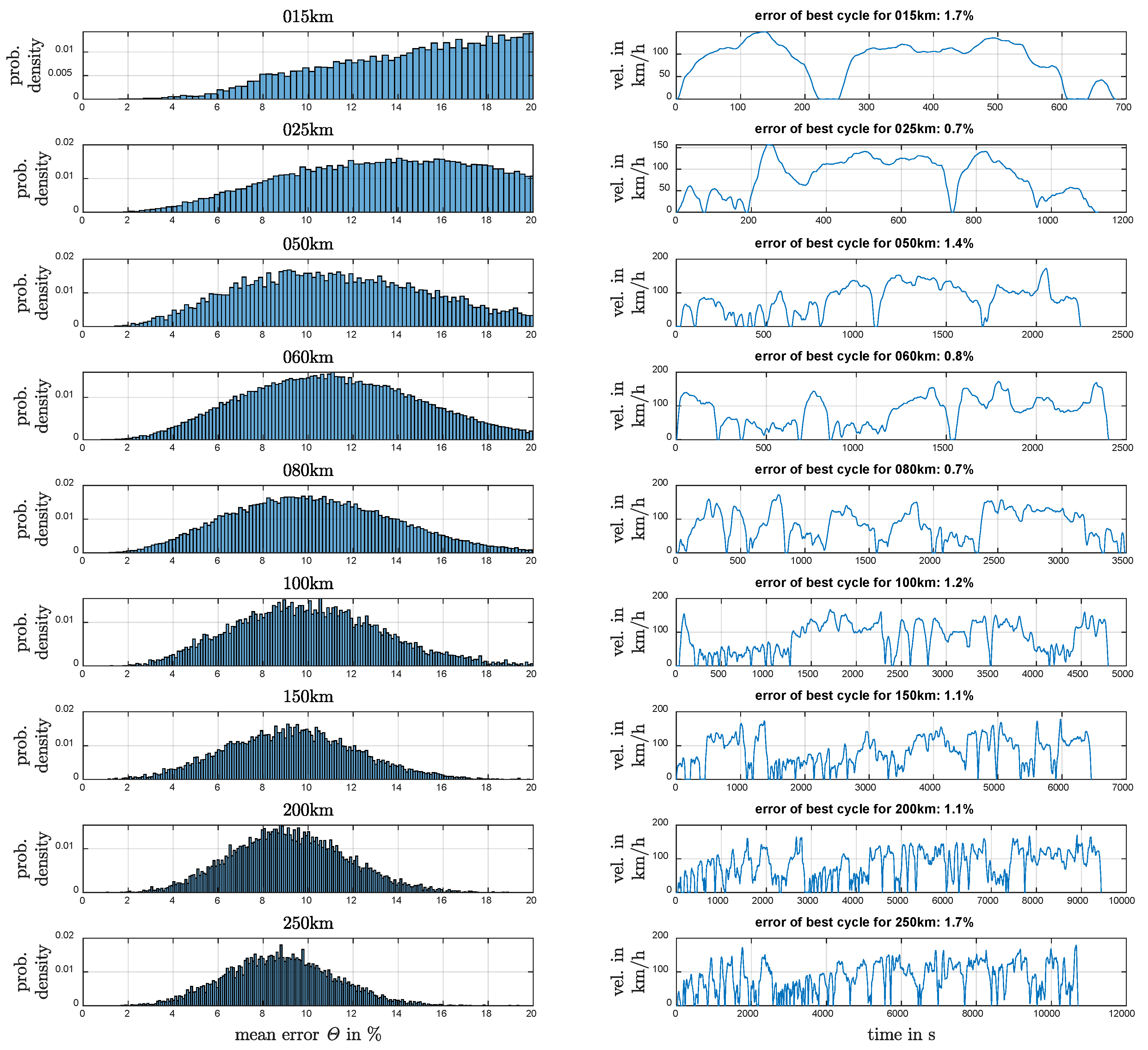
  16. Esser, A.; Zeller, M.; Foulard, S.; Rinderknecht, S. Stochastic Synthesis of Representative and Multidimensional Driving Cycles. SAE Int. J. Alt. Power. 2018, 7, 263–272. [Google Scholar] [CrossRef]
  17. OpenStreetMap. Available online: www.openstreetmap.org (accessed on 12 October 2018).
  18. Wipke, K.B.; Cuddy, M.R.; Burch, S.D. ADVISOR 2.1: A user-friendly advanced powertrain simulation using a combined backward/forward approach. IEEE Trans. Veh. Technol. 1999, 48, 1751–1761. [Google Scholar] [CrossRef]
  19. An, J.; Binder, A. Operation Strategy with Thermal Management of E-Machines in Pure Electric Driving Mode for Twin-Drive-Transmission (DE-REX). In Proceedings of the 2017 IEEE Vehicle Power and Propulsion Conference (VPPC), Belfort, France, 14–17 December 2017; IEEE: Piscataway, NJ, USA, 2017; pp. 1–6. [Google Scholar]
  20. An, J.; Binder, A. Permanent magnet synchronous machine design for hybrid electric cars with double e-motor and range extender. Elektrotech. Inftech. 2016, 133, 65–72. [Google Scholar] [CrossRef]
  21. Paganelli, G.; Delprat, S.; Guerra, T.M.; Rimaux, J.; Santin, J.J. Equivalent Consumption Minimization Strategy for Parallel Hybrid Powertrains. In Proceedings of the IEEE Vehicular Technology Conference, Birmingham, AL, USA, 6–9 May 2002. [Google Scholar]
  22. Serrao, L.; Onori, S.; Rizzoni, G. ECMS as a realization of Pontryagin’s minimum principle for HEV control. In Proceedings of the IEEE American Control Conference, St. Louis, MO, USA, 10–12 June 2009. [Google Scholar]
  23. Rinderknecht, S.; Esser, A.; Schleiffer, J.-E.; Eichenlaub, T. Comparative Real-Driving Optimization of Drivetrain Concepts regarding the Ecological Impact—A Big Data Approach for the Fleet. In Proceedings of the eDSIM Conference, Darmstadt, Germany, 25–26 September 2018. [Google Scholar]
  24. Beetz, K.; Kohle, U.; Eberspach, G. Beheizungskonzepte für Fahrzeuge mit Alternativen Antrieben. ATZ Automobiltechnische Zeitschrift 2010, 112, 246–249. [Google Scholar] [CrossRef] [Green Version]
  25. Großmann, H. Pkw-Klimatisierung. Physikalische Grundlagen und Technische Umsetzung; Springer: Berlin/Heidelberg, Germany, 2010. [Google Scholar]
Figure 1. Distribution of the daily mean ambient temperatures measured in Darmstadt by “Deutscher Wetterdienst” [14] during the period from Jan. 2013 until Jan. 2017 with a fitted normalized distribution in (a) and distribution of trip distances of passenger cars from [15] within Germany in (b).
Vehicles 01 00005 g001
Figure 2. Database of driving data used for this study as an input for the cycle synthesis procedure [16]. In (a), the considered tracks from the region around the cities of Darmstadt and Frankfurt in Germany are illustrated. In (b), the occurrence frequency of driving states in the velocity-acceleration plane is plotted.
Vehicles 01 00005 g002
Figure 3. On the left, the error distributions regarding the criteria set θ of the 10,000 synthesized cycles are displayed for each trip distance. There is a bigger variation in cycle quality for shorter trips because it is more difficult to satisfy all evaluation criteria in this case. On the right, the best cycles for each trip distance and the corresponding errors are displayed, which correspond to the best value of the error distribution on the left from the same row.
Vehicles 01 00005 g003
Figure 4. Exemplary outputs of the primary consumption model for the plug-in hybrid electric vehicle (PHEV) on a representative driving cycle with a trip distance of 100 km. In (a), the time-resolved graphs of vehicle velocity, gear, internal combustion engine (ICE) and electrical traction machine (EM) torques, state of charge (SOC) are shown. In (b) and (c), the chosen operating points of ICE and EM, with the corresponding operation conditions including boosting and shifting, are shown in the brake specific fuel consumption (BSFC) and efficiency maps, respectively.
Vehicles 01 00005 g004
Figure 5. The figure shows the fuel consumption in dependency of ambient temperature and trip distance for an ICEV. It shows that the overall dependency in temperature is small at a maximum derivation of 5.5% whilst the dependency in trip distance of 1.9% is even lower. The WLTP consumption without secondary energy demands is simulated at 4.17 l/100 km and is thus at least 20.6% lower.
Vehicles 01 00005 g005
Figure 6. The figure shows the electricity consumption in dependency of ambient temperature and trip distance for a BEV. It shows that the overall dependency in trip distance is higher than in case of an ICEV at a maximum derivation of 11.0% whilst the dependency in ambient temperature is even higher at a maximum of 22.7%. The WLTP electricity consumption without secondary energy demands is simulated at 12.9 kWh/100 km and is thus at least 35.5% lower.
Vehicles 01 00005 g006
Figure 7. The figure shows the electricity (a) as well as the fuel (b) consumption as a function of ambient temperature and trip distance for the PHEV. Since the operating strategy tries to fully deplete the battery, the electrical energy consumption is highly sensitive to trip distance. Below the electrical range of the vehicle, the electric consumption is much higher and shows a strong dependency on ambient temperature, similar to the BEV. Above the electrical range, the electric consumption is almost constant with respect to ambient temperature but decreases with higher trip distances because of the increasing use of fuel.
Vehicles 01 00005 g007
Table 1. Exemplary calculation of the overall error of the best synthesized cycle at a trip distance of 80 km for all single criteria θ i and the criteria set θ. The results of all error calculations are presented in Figure 3.
CriteriaProfileSingle CycleError
θ 1 23.06722.9870.3%
θ 2 150.481150.2330.1%
θ 3 0.20840.21051.0%
θ 4 577.369582.6410.9%
θ 5 0.5840.5870.5%
θ 6 0.12230.12360.1%
θ 0.66%
Table 2. Main parameters of the defined vehicle drivetrain concepts.
Main ParametersICEVBEVPHEV
ICE power in kW96~85
EM power in kW~300120
Battery capacity in kWh~6020
Number of gears717
Total mass in kg110916351358
Necessary starting torque in Nm165624422028
Typical electrical power rating of HVAC system in W [24]400–200060003500
Table 3. Heating ventilation and air conditioning (HVAC) technology depending on vehicle concepts where hooks in brackets (✓) are not considered within this work.
HVAC TechnologyICEVBEVPHEV
Heat exchanger heating
PTC element heating(✓)
Heat pump heating(✓)
Heat pump cooling

