Abstract
Despite the importance of demonstrating and evaluating how structural equation modeling (SEM), exploratory structural equation modeling (ESEM), and Bayesian structural equation modeling (BSEM) work simultaneously, research comparing these analytic techniques is limited with few studies conducted to systematically compare them to each other using correlated-factor, hierarchical, and bifactor models of personality. In this study, we evaluate the performance of SEM, ESEM, and BSEM across correlated-factor, hierarchical, and bifactor structures and multiple estimation techniques (maximum likelihood, robust weighted least squares, and Bayesian estimation) to test the internal structure of personality. Results across correlated-factor, hierarchical, and bifactor models highlighted the importance of controlling for scale coarseness and allowing small off-target loadings when using maximum likelihood (ML) and robust weighted least squares estimation (WLSMV) and including informative priors (IP) when using Bayesian estimation. In general, Bayesian-IP and WLSMV ESEM models provided noticeably best model fits. This study is expected to serve as a guide for professionals and applied researchers, identify the most appropriate ways to represent the structure of personality, and provide templates for future research into personality and other multidimensional representations of psychological constructs. We provide Mplus code for conducting the demonstrated analyses in the online supplement.
1. Introduction
Factor analysis has served as a critical tool for understanding the nature of constructs included in personality inventories. Over the years, factor analysis techniques have advanced from simple exploratory analyses to more sophisticated approaches that include (a) confirmatory factor analyses (CFAs); (b) estimation procedures that adjust for non-normal distributions, correct for ordinal-level data, and enhance model convergence; (c) extensions of simple structure models, also called independent-clusters models (IC-CFA; [1]), to allow for cross-loadings for non-targeted items via small-variance priors.
Maximum likelihood (ML) estimation is commonly used in factor analytic models but is affected by scale coarseness, whereas weighted least squares estimation with means and variances adjusted (WLSMV) corrects for such effects (e.g., [2,3]). Bayesian estimation allows for the incorporation of prior information in testing models (e.g., [4,5]). Traditional factor analytic procedures have forced off-target loadings to equal zero, but more recent exploratory structural equation modeling (ESEM) techniques have allowed such loadings to vary from zero to improve model fit and represent constructs more realistically ([6]).
Despite the importance of demonstrating how these CFA models estimated under maximum likelihood (CFA ML) and CFA models estimated under mean-variance adjusted weighted least squares (CFA WLSMV), exploratory structural equation modeling under maximum likelihood (ESEM ML), exploratory structural equation modeling under mean-variance adjusted weighted least squares (ESEM WLSMV), and Bayesian structural equation modeling (BSEM) analytical dimensions work, research comparing these analytic techniques simultaneously is limited with no studies to the best of our knowledge conducted to systematically compare them to each other using more complex correlated-factor, hierarchical factor, and bifactor models of personality or other related constructs.
In this study, we demonstrate how structural equation modeling (SEM) can be applied with different estimation methods (maximum likelihood (ML) vs. weighted least squares with mean and variance adjusted (WLSMV) vs. Bayesian and factor loading constraints (exploratory structural equation modeling; ESEM)) to find the types of procedures that best represent the theoretical framework of personality using online data for 447,500 respondents from the International Personality Item Pool (IPIP) database ([7]). The present study is focused on the most recent advances in factor analytic procedures to determine their relative effectiveness in best representing constructs measured by a personality inventory. The present analyses are expected to provide templates for future research into personality and other similar multidimensional representations of psychological constructs by implication.
The remainder of this paper is structured as follows: first, we provide an overview of factor analytic techniques including exploratory factor analysis, confirmatory factor analysis, exploratory structural equation modeling, and Bayesian structural equation modeling with an emphasis on correlated-factor, hierarchical, and bifactor structures. Next, we discuss (a) the methods used, data, and sample; (b) the results; (c) the discussion and implications; (d) recommendations for future studies; (e) limitations; and (f) conclusions.
2. An Overview of Factor Analytic Techniques
The primary goal of factor analysis is to determine the number and nature of latent variables or factors that explain variation and covariation among observed scores ([8]). Two main kinds of factor analysis fall under the umbrella of Thurstone’s (1947) [9] common factor model: exploratory factor analysis (EFA) and confirmatory factor analysis (CFA; [10,11]). Both methods seek to account for observed relationships among a set of indicators with a smaller set of latent variables or factors but are fundamentally different in other ways ([8,12]).
2.1. Exploratory Factor Analysis (EFA)
EFA is data-driven in the sense that the number of factors or the pattern of associations between the latent factors and the indicators need not be initially specified. EFA is used as an exploratory or descriptive tool to find an appropriate number of common factors and to determine which observed measures serve as the best indicators of the latent factors by the size and magnitude of factor loadings ([8,12]).
However, EFA has several shortcomings. These generally include the absence of fit indexes, being data-driven rather than theory-driven, the inability to account for method effects, confounding measurement error and indicator specificity, and the absence of procedures for testing measurement invariance and formal theoretical models ([13]). Confirmatory factor analysis is intended to alleviate these shortcomings.
2.2. Confirmatory Factor Analysis (CFA)
Confirmatory factor analysis (CFA) is a structural equation modeling (SEM) procedure that quantifies associations between observed measures or indicators (e.g., items) and latent variables or factors ([8]). CFA is a common statistical approach to analyzing complex multidimensional structures underlying personality inventories, including correlated-factor, hierarchical, and bifactor models. CFA is theory-driven, but it often fails to achieve acceptable model fit and can produce substantial parameter biases in the estimation of factor loadings and correlations because of its restrictive assumptions of exact zero cross-loadings and residual covariances (e.g., [8,12,14,15]). The CFA model links the observed indicators to the latent factors via the measurement equation
where indexes observations, is a vector of observed indicators, is a vector of intercepts, is a vector of latent variables, is a vector of measurement errors, and is a matrix of factor loadings that links the latent variables to the observed indicators. Under standard assumptions of the CFA model, and are normally distributed and independent, implying that and , with denoting the mean vector of the latent variables, is a factor covariance matrix, and is the residual covariance matrix.
Common CFA Models: Correlated-Factor, Hierarchical, and Bifactor Models
In this study, three types of CFA models including the correlated-factor, hierarchical, and bifactor models are relevant (see Figure 1). Within correlated-factor CFA models, factors are typically intercorrelated, but the researcher does not analyze the directions or patterns of factor interrelationships. Hierarchical factor analysis extends such modeling by further investigating higher-order factors that might account for intercorrelations among lower-order factors. Hierarchical CFA models, as the name implies, are useful when theory dictates that constructs are related in a hierarchical fashion in which lower-order factors account for the intercorrelations among observed indicators and higher-order factors in turn account for interrelationships among lower-order factors. As a result, the hierarchical model is more parsimonious but can fit the data no better than the correlated-factor model. Hierarchical models must include at least three first-order factors to differ from correlated-factor models. Additionally, first-order factors should have at least three indicators ([8,12,15,16,17]).
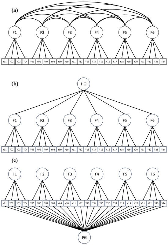
Figure 1.
Examples of correlated-factor, hierarchical, and bifactor measurement models. Note: F = factor; FG = general factor; HO = hierarchical factor. In (a), the correlated-factor model, covariation in the observed indicators is explained by six interrelated factors; in (b), the hierarchical model, covariation in the observed indicators is captured by lower-order factors whose interrelationship is in turn captured by the hierarchical factor; in (c), the bifactor model, covariation in the observed indicators is primarily captured by a general factor with the specific factors capturing additional covariation not captured by the general factor. For simplicity, residual variances and intercepts are omitted.
Bifactor (also known as nested-factor or general-specific) models serve as alternatives to hierarchical models ([17]). Such models have a latent structure that includes a general factor that accounts for the commonality among all indicators and independent group factors that represent systematic variance specific to nested and non-overlapping subsets of indicators ([8,12,16,18]). Unlike correlated-factor models, bifactor and hierarchical models both assume that global factors in addition to more specific factors explain covariation in observed scores ([13]).
Chen et al. (2006) [17] enumerated the following advantages of the bifactor model. First, the bifactor model can work as a baseline model to be compared to the second-order model through a likelihood ratio test because the second-order model is nested within the bifactor model ([19,20]). Second, the bifactor model can be used to assess the importance of domain-specific factors that are orthogonal to the general factor. For example, with Spearman’s (1927) [21] original conception of general and domain-specific factors, he assumed that there was a factor representing general intelligence as well as domain-specific factors reflecting separate abilities such as verbal, spatial, mathematical, and analytic.
Third, bifactor models show the strength of association between the specific group factors and their corresponding indicators with the effects of the general factor partialed out and vice versa. This is not the case with the hierarchical model because interpretations are level specific. Finally, the bifactor model can be used to predict outcomes using both the general and group factors while they mutually control for each other’s effects. This cannot be done with the second-order model because the second-order factors directly affect the first-order factors and thus residual variances of the first-order factors reflect the variability of the domain-specific factors that are not accounted for by the second-order factors ([8,17] Brown, 2015; Chen et al., 2006).
Despite the interpretative advantages of the three types of CFA models described here, they are not without their shortcomings and often fail to yield acceptable fits ([14] Marsh et al., 2014). The likelihood of this occurring typically increases as the number of items representing each factor increases ([22,23,24] Booth and Huges, 2014; Marsh et al., 2005; Marsh et al., 2010a). Misfit can occur because items typically do not exclusively represent the factors to which they are linked. In EFA, all cross-loadings are freely estimated to indicate potential systematic associations with other constructs, but such cross-loadings are forced to be zero in the basic IC-CFA models discussed here. Such restrictions also can result in inflated correlations among CFA factors, poor discriminant validity, and less accurate structural parameter estimates in misspecified SEMs ([6,14,15] Asparouhov and Muthén, 2009; Marsh et al., 2014; Morin et al., 2016).
2.3. Exploratory Structural Equation Modeling
Exploratory structural equation modeling (ESEM) was proposed by Asparouhov and Muthén (2009) [6] as an alternative method to solve the problems described in the previous paragraph by merging methodological advantages of CFA, SEM, and EFA to allow for assessment of goodness-of-fit, tests of multiple-group invariance, longitudinal differential item functioning, higher-order factor structures, growth modeling, and other applications ([6,13,14,24] Asparouhov and Muthén, 2009; Marsh et al., 2009, 2010a; Marsh et al., 2014).
ESEM Correlated-Factor, Hierarchical, and Bifactor Models
An appealing attribute of the ESEM framework is that it is applicable to the correlated-factor, hierarchical, and bifactor models of interest to this study, and has been applied in numerous studies (see, e.g., [15,25,26,27,28] Litalien et al., 2017; Morin et al., 2016; Perera, 2016; Sánchez-Oliva et al., 2017; Tóth-Király et al., 2018). Perera (2016) [26] investigated the construct validity of the Social Provisions Scale data using correlated-factor, bifactor, and higher-order ESEM models and found that the bifactor ESEM model outperformed other ESEM and IC-CFA models, which links each item to one factor only, with respect to model fit. Perera also found that the correlated-factor ESEM model produced much lower factor correlations than those in the corresponding IC-CFA model. Tóth-Király et al. (2018) [28] examined the multidimensionality of responses to the Basic Psychological Need Satisfaction and Frustration inventory using bifactor ESEM and found that most of the bifactor ESEM models achieved an acceptable level of model fit. Figure 2 illustrates an example of exploratory SEM correlated-factor, hierarchical, and bifactor models, respectively.
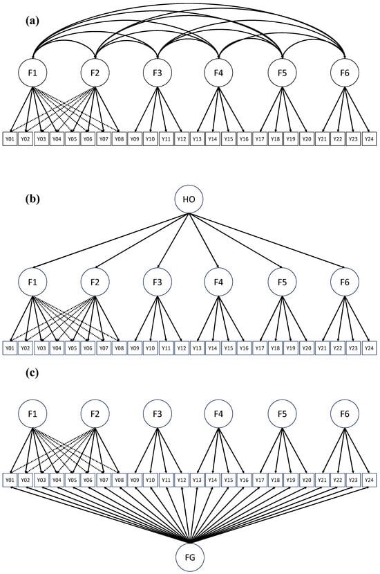
Figure 2.
Examples of exploratory SEM (a) correlated-factors, (b) hierarchical, and (c) bifactor models. Note: F: factor; FG: general factor; HO: higher-order factor. For simplicity and illustrative purposes, the figures above only contain a subset of cross-loadings (represented with the dashed lines).
2.4. Estimation Methods
Maximum Likelihood vs. Weighted Least Squares
With maximum likelihood (ML) estimation in factor modeling, observed item scores are assumed to fall on a continuous equal-interval scale that follows a multivariate normal distribution ([3,29,30] Beauducel and Herzberg, 2006; Li, 2016; Rhemtulla et al., 2012). When data are categorical or ordinal, diagonally weighted least squares procedures such as weighted least squares estimation with means and variances adjusted (WLSMV) can be used to correct for scale coarseness effects ([2,3] Beauducel and Herzberg, 2006; Muthén, 1993). WLSMV is an asymptotically distribution-free estimation procedure involving polychoric correlation matrices ([2] Muthén, 1993). The WLSMV estimator has been shown to produce better results when ordinal indicators are employed within SEMs ([3,31] Beauducel and Herzberg, 2006; Nussbeck et al., 2006) and when continuous and categorical indicators are used with multilevel SEMs ([32,33] Hox et al., 2010; Nylund et al., 2007).
2.5. Bayesian Structural Equation Modeling
Bayesian structural equation modeling (BSEM) has been proposed as an alternative approach to traditional CFA and SEM to improve model fit and provide less restrictive and more realistic presentations of the nature of constructs measured within personality inventories ([6,34] Asparouhov and Muthén, 2009; Muthén and Asparouhov, 2012). The term BSEM encompasses an extensive variety of Bayesian analyses conducted in SEM with numerous prior distributions ([35] Liang, 2020). BSEM is less restrictive than maximum likelihood procedures and uses prior information to reflect a researcher’s theories or prior knowledge in a way that the previously discussed estimation procedures do not. In contrast to BSEM, ML procedures rely on large-sample theory and normality assumptions ([34,36] Levy and Choi, 2013; Muthén and Asparouhov, 2012). BSEM is not based on such assumptions and can be used with small samples and in situations where ML estimates do not converge or yield counterintuitive results (e.g., [37,38,39] Heerwegh, 2014; Liang et al., 2020; van de Schoot et al., 2015).
Rooted in Bayes’ theorem, BSEM treats a vector of model parameters as random variables that are assigned a prior distribution according to a researcher’s previous knowledge, beliefs, or assumptions. The elements in include, but are not limited to, item intercepts, factor loadings, residual variances and factor covariances. The distributions are collectively denoted as ) and are referred to as priors. Bayesian inference combines the prior distribution ) and the likelihood of the observed data ) (i.e., the SEM model of interest) to produce the posterior distribution, denoted by ) ([5] Levy and Mislevy, 2017), which reflects updated knowledge about in light of the observed data. Bayes’ theorem says that the posterior distribution is given by
where is the marginal distribution of the observed data after the parameters have been integrated over their respective parameter space. Except for simple cases, the marginal distribution of the observed data are generally not available in analytic form, however, because it is constant with respect to the parameter vector , it is not needed in Bayesian computations.
Previous research on BSEM has found that a Bayesian approach provides bettermodel fit than CFA/SEM ([34] Muthén and Asparouhov, 2012). In addition, BSEM is also more flexible when the models are complex with smaller sample sizes of respondents in comparison to ESEMs which typically require larger samples to provide trustworthy results ([35,40] Liang, 2020; Reis, 2017).
2.5.1. Types of Priors
The prior distribution represents theories and previous knowledge or beliefs that a researcher has about the parameter values before gathering new data and conducting a new study ([34,41] Kaplan, 2014; Muthén and Asparouhov, 2012). Priors are specified for each of the CFA model parameters. They can be informative (small prior variance) or non-informative (large prior variance; also called vague or diffuse).
Informative priors are used when there are sufficient previous findings about the nature of scales and shapes of distributions ([42,43] Kaplan and Depaoli, 2012; Zyphur and Oswlad, 2015). BSEM provides a means to shrink noise parameters (e.g., trivial cross-loadings) toward zero in a sparse factor loading matrix. Many cross-loadings are constrained to zero, and only a few important or theoretically relevant cross-loadings are typically allowed to be non-zero ([35,44,45] Bhattacharya and Dunson, 2011; Kaufmann and Schumacher, 2017; Liang, 2020). Informative priors on small-sized parameters such as cross-loadings are assigned and manipulated to achieve shrinkage. Shrinkage priors are intended to diminish the noise parameters (e.g., trivial cross-loadings) toward zero for the purpose of generating a more parsimonious factor model while keeping estimates strong for the signal parameters (e.g., targeted loadings and non-trivial targeted cross-loadings; [35,38] Liang, 2020; Liang et al., 2020).
The small-variance normal prior is one of the shrinkage priors commonly used among various kinds of distributions in BSEM and available in Mplus ([34,40,46] Muthén and Asparouhov, 2012; Price, 2017; Reis, 2017). In BSEM with small-variance normal distribution priors (BSEM-N), major loadings are estimated in a confirmatory approach by being assigned non-informative priors (e.g., N (0, 1010)) or weakly informative priors if prior information is presented from past analyses. Cross-loadings are estimated in an exploratory way and penalized by being assigned shrinkage priors with a mean of zero and a small variance ([35] Liang, 2020). For example, utilizing a normal prior of N (0, 0.01) suggests “the prior belief that a 95% chance the true cross-loading falls between −0.196 and 0.196” ([38] Liang et al., 2020, p. 876). In comparison to the independent clusters model CFA, which allows each item to load on one factor and sets all the cross-loadings to zero ([13] Marsh et al., 2009), Bayesian estimation is flexible in estimating models by regulating the variability in cross-loadings through controlling prior distributions. This enables models that are not computed by frequentist methods such as ML to be estimated ([38] Liang et al., 2020).
Non-informative priors are employed when we do not possess sufficient prior knowledge or information or have consistent findings or theories to yield posterior inferences. This lack of information is still important to quantify to represent our cumulative understanding of an imminent problem. Non-informative priors are regarded as a standard method to quantify the lack of prior information.
One type of commonly used non-informative prior distribution is the uniform (flat) distribution. This prior is less informative (i.e., flatter) than other types of priors, so it allows the data to take over the estimation of posteriors via their likelihood ([47,48] Gill, 2008; Kass and Wasserman, 1996). This distribution indicates that, before any data are assembled, no parameter values are more plausible than others. A prior distribution with a large variance, such as a normal distribution with a mean and variance , serves a similar purpose. This variance makes the prior probability distribution of the parameter values almost flat, which is the default setting in Mplus (see [49,50] Asparouhov and Muthén, 2010; Muthén, 2010).
The choice of the prior distribution is challenging ([43,51] Xiao et al., 2019; Zyphur and Oswlad, 2015) because priors may influence the results in different and potentially misleading ways ([52,53] van de Schoot and Depaoli, 2014; van Erp et al., 2018). For example, researchers (e.g., [34,53] Muthén and Asparouhov, 2012; van Erp et al., 2018) have found that the use of improper priors and the large prior variance can result in model convergence problems and unstable estimates. Van Erp et al. (2018) [53] recommended that several default priors be used to evaluate the effects of the choice of the prior on model estimation.
The Markov chain Monte Carlo (MCMC) algorithm is often applied to empirically approximate posterior distributions. The words Monte Carlo mean that a simulation process with sampling, generating, and drawing is applied. The word chain indicates that the random values are drawn by being linked and taking place sequentially. Thus, MCMC iteratively draws many samples from posterior distributions of unknown model parameters. When MCMC chains converge to a stationary distribution, Bayesian parameter estimates can be generated based on summary statistics (e.g., mean, mode, standard deviation, median, and quantiles) of the posterior distributions ([4,5,35,42] Gelman et al., 2014; Kaplan and Depaoli, 2012; Levy and Mislevy, 2017; Liang, 2020).
2.5.2. Bayesian Model Fit Evaluation
Model goodness-of-fit indices and information criteria (IC) used in conventional SEMs have also been adapted for use in BSEM. These include the Bayesian root mean square error of approximation (BRMSEA; [7] Hoofs et al., 2018), the Bayesian comparative fit index (BCFI), and the Bayesian Tucker–Lewis index (BTLI; [54] Garnier-Villarreal and Jorgensen, 2020). BRMSEA, BCFI, and BTLI indices of model fit are based on discrepancies between actual and replicated data at each MCMC iteration in a similar way to the posterior predictive model checking technique (PPMC; e.g., [55] Gelman et al., 1995). PPMC replicates a dataset with the same sample size as the observed data at every MCMC iteration and quantifies a posterior predictive p-value (PPp; [56] Meng, 1994) as the proportion of iterations where the fit statistic calculated based on the observed data does not exceed the fit statistic obtained from the replicated data. PPMC implies that the discrepancy between the observed and replicated data should be minimal when the model fits the data ([34,42] Kaplan and Depaoli, 2012; Muthén and Asparouhov, 2012). BRMSEA indices have been shown effective in large samples (). Unlike most frequentist equivalents, Bayesian adaptions of fit indices also include credibility intervals to quantify their uncertainty ([54] Garnier-Villarreal and Jorgensen, 2020).
In keeping with cutoff criteria for acceptable model fit within a frequentist structural equation modeling framework stated earlier, RMSEAs less than 0.06 indicate excellent fit, and values less than 0.08 are acceptable with sample sizes greater than or equal to 1000. In contrast, the application of traditional cutoff values for BCFI and BTLI is not endorsed by Garnier-Villarreal and Jorgensen (2020) [54] because the criteria were not applicable to all samples.
3. Research on IPIP-NEO-120
The International Personality Item Pool—Neuroticism, Extraversion, and Openness (IPIP-NEO-120) questionnaire is a public domain 120-item inventory that assesses personality traits under the Big Five model. The domain scales (Openness, Conscientiousness, Extraversion, Agreeableness, and Neuroticism) have 24 items each with six nested four-item facet subscales under each domain ([57] Johnson, 2014). The IPIP-NEO-120 was assembled by Johnson as an abbreviated version of the 300-item IPIP-NEO inventory ([58] Goldberg, 1999) and is intended to measure the same constructs assessed by the original 240-item NEO Personality Inventory (NEO PI-R; [59] Costa and McCrae, 1992). To measure personality more efficiently, researchers have created several reduced-length forms of the IPIP-NEO-300, including the IPIP-20, IPIP-50, IPIP-100, and IPIP-NEO-120, but only the IPIP-NEO-120 measures all six facets nested under each of the Big Five domains. The IPIP-NEO-120 is available from the IPIP website (http://ipip.ori.org), accessed on 28 November 2023.
Reliability and Validity Evidence of the IPIP-NEO-120
Because the IPIP-NEO-120 was developed recently ([57] Johnson, 2014), empirical studies investigating its psychometric properties are limited. The following summary of findings from those studies (e.g., [57,60,61,62,63] Giolla and Kajonius, 2019; Johnson, 2014; Kajonius and Giolla, 2017; Kajonius and Johnson, 2018, 2019) verifies that scores from the IPIP-NEO-120 show solid evidence for reliability and validity despite its reduced length.
The reliability indices of the IPIP-NEO-120 are commonly reported at both domain and facet levels. Overall, alpha coefficients ranged from 0.81 to 0.92 for domain scales and from 0.47 to 0.89 for facet scales. In general, the mean alpha coefficients for domain scales were higher than those for facet scales ([57,60,61,62,63,64,65,66] Giolla and Kajonius, 2019; Johnson, 2014; Kajonius and Giolla, 2017; Kajonius and Johnson, 2018, 2019; Lace et al., 2019, 2020a, 2020b).
The convergent validity evidence of the IPIP-NEO-120 was reported in two studies. [57] Johnson (2014) evaluated the convergent validity of the IPIP-NEO-120 in the Eugene-Springfield sample by correlating subscale scores with those for the NEO PI-R ([59] Costa and McCrae, 1992). Correlation coefficients among IPIP-NEO-120 and NEO PI-R ([59] Costa and McCrae, 1992) domain scores ranged from 0.76 to 0.87 (M = 0.82) and among facet scores from 0.53 to 0.76 (M = 0.66). Lace et al. (2019) [65] also reported convergent concurrent validity coefficients of the IPIP-NEO-120 Anxiety and Depression scores with Anxiety and Depression scores from the Kessler Psychological Distress Scale (K10) with correlations of 0.65 for Anxiety and 0.75 for Depression, respectively.
Factor structures for IPIP-NEO-120 scale scores were also investigated using CFA, EFA, and maximum likelihood estimation in two studies ([61,63] Kajonius and Giolla, 2017; Kajonius and Johnson, 2019). Kajonius and Giolla (2017) [61] used a worldwide sample of 130,602 respondents from 22 countries to examine hierarchical factor models using confirmatory factor analysis with maximum likelihood estimation for each of the five global domains. They reported comparative fit indices (CFIs) ranging from 0.87 to 0.92 for Neuroticism, 0.75 to 0.89 for Extraversion, 0.76 to 0.89 for Openness, 0.84 to 0.91 for Agreeableness, and 0.89 to 0.94 for Conscientiousness across 22 countries.
As another example, Kajonius and Johnson (2019) [63] initially confirmed the five factors of the IPIP-NEO-120 using exploratory factor analysis with maximum likelihood estimation based on a sample of 320,128 respondents living in the United States. They then compared hierarchical and bifactor confirmatory factor analysis models utilizing maximum likelihood estimation for each of the IPIP-NEO-120 global domains. They found that bifactor models fit better than hierarchical models with the largest differences in CFIs between bifactor and hierarchical models observed for Extraversion (0.91 vs. 0.88) and Agreeableness (0.93 vs. 0.87).
4. Significance of the Current Study
Recent research into ESEM and BSEM has been primarily focused on simple factor analytic models and generally shows that these procedures better fit data than CFAs (e.g., [51,67] Guo et al., 2019; Xiao et al., 2019). Also, factor analytic studies of IPIP-NEO-120 responses ([61,63] Kajonius and Giolla, 2017; Kajonius and Johnson, 2019) were limited to hierarchical and bifactor confirmatory factor analysis models using maximum likelihood estimation. For example, Guo et al. (2019) [67] evaluated and contrasted single-factor models of CFA, ESEM, and BSEM using the 60-item NEO Five-Factor Inventory (NEO-FFI; [59] Costa and McCrae, 1992); Muthén and Asparouhov (2012) [34] compared five-factor models of CFA and BSEM using Big Five personality data from the British Household Panel Study; and Kim and Wang (2021) [68] assessed the factor structure of data from the Positive and Negative Affect Schedule (PANAS; [69] Watson et al., 1988) employing correlated-factor and bifactor models of CFA, ESEM, and BSEM. In all instances, ESEM and BSEM performed better than CFA.
Absent from these studies are weighted least squares with mean and variance adjusted estimation (WLSMV), exploratory structural equation modeling, and Bayesian structural equation modeling analyses. Limited research involved comparisons of CFA, ESEM, and BSEM simultaneously, focusing only on simple factor analytic models for the Big Five personality models (e.g., [34,67,68] Guo et al., 2019; Kim and Wang, 2021; Muthén and Asparouhov, 2012). To the best of our knowledge, no research has been conducted within more complex correlated-factor, hierarchical, and bifactor frameworks with the IPIP-NEO-120. Because the IPIP-NEO-120 was recently developed, evidence supporting the reliability and validity of its scores is quite limited. The present study is focused on the most recent advances in factor analytic procedures to determine their relative effectiveness in best representing constructs measured by a personality inventory, allowing replication of analyses within a distinct domain of personality.
5. Illustrations of SEM, ESEM, and BSEM Techniques Using IPIP-NEO-120 Agreeableness Scale
In this study, we demonstrate and evaluate the effects of SEM estimation methods (maximum likelihood (ML) vs. weighted least squares with mean and variance adjusted (WLSMV) vs. Bayesian estimation) and factor loading constraints (exploratory structural equation modeling: ESEM) on model fit in correlated-factor, hierarchical, and bifactor models using IPIP-NEO-120 Agreeableness Scale. The following three research questions will guide this study.
- RQ1.
- To what extent do parameter estimation methods (SEM ML, WLSMV, and Bayesian SEM) affect model fit for correlated-factor, bifactor, and hierarchical factor models?
- RQ2.
- To what extent do factor loading constraints (allowing vs. restricting weak off-target loadings; ESEM vs. CFA) affect model fit for correlated-factor, bifactor, and hierarchical factor models?
- RQ3.
- To what extent will the use of different priors in BSEM affect model fit for correlated-factor, bifactor, and hierarchical factor models?
6. Methods
6.1. Data and Measure
IPIP-NEO-120
The IPIP-NEO-120 ([57] Johnson, 2014) is a 120-item personality inventory that measures the Big Five personality factors (Agreeableness, Conscientiousness, Extraversion, Neuroticism, and Openness to Experience). Each of the five domain scales has six nested four-item facet subscales. The Agreeableness subscale consists of 24 items measuring levels of trust, morality, altruism, cooperation, modesty, and sympathy. The Conscientiousness subscale has 24 items focused on self-efficacy, orderliness, dutifulness, achievement-striving, self-discipline, and cautiousness. The Extraversion subscale consists of 24 items with facets for friendliness, gregariousness, assertiveness, activity level, excitement-seeking, and cheerfulness. The Neuroticism subscale has 24 items that measure anxiety, anger, depression, and vulnerability. The Openness to Experience subscale includes 24 items for the facets of imagination, artistic interests, emotionality, and liberalism ([57] Johnson, 2014).
Items are answered using a five-point Likert-type rating scale in which 1 = Very Inaccurate, 2 = Moderately Inaccurate, 3 = Neither Accurate nor Inaccurate, 4 = Moderately Accurate, and 5 = Very Accurate (see Figure 3), with possible scores ranging from 24 to 144 for each 24-item domain scale, and from 4 to 20 for each facet subscale. Missing values are coded as 0. The IPIP-NEO-120 consists of 65 positively phrased and 55 negatively phrased items. Among the domain scales, 29%, 46%, 75%, 71%, and 50% are positively phrased for Agreeableness, Conscientiousness, Extraversion, Neuroticism, and Openness to Experience, respectively. Negatively phrased items are reverse scored by recoding (1 = 5, 2 = 4, 4 = 2, 5 = 1), and this recoding is automatically done after respondents finish the questionnaire so that users need not do so themselves ([57] Johnson, 2014). For illustrations, we used data from the Agreeableness subscale.

Figure 3.
Five-point Likert-Type Rating Scale of IPIP-NEO-120.
6.2. Sample
Participants included in the study sample consisted of 447,500 respondents from the United States who voluntarily completed the International Personality Item Pool NEO-120 questionnaire (IPIP-NEO-120; [57] Johnson, 2014) at the IPIP website (data publicly available via the Open Source Framework at https://osf.io/tbmh5/wiki/home/) accessed on 28 November 2023. It consisted of 39% male (N = 174,707) and 61% female (N = 272,793) respondents who had an average age of 24.93 years (SD = 10.29).
6.3. Descriptive Statistics
Preliminary analyses included descriptive statistics for the Agreeableness domain and their facet scores (means and standard deviations) and conventional reliability estimates (alpha and omega; see Table 1). Item-scale means ranged from 3.10 to 4.13. The mean item-scale standard deviation across all facets was 0.82. Alpha reliability estimates ranged from 0.70 to 0.84 (overall M = 0.85 for the domain, and M = 0.73 across facets). Omega coefficients ranged from 0.70 to 0.85 (overall M = 0.90 for the domain, and M = 0.74 across facets).

Table 1.
Descriptive Statistics and Conventional Reliability Estimates for IPIP-NEO-120 Agreeableness Facet Scores (N = 447,500).
6.4. Data Analyses
Data analyses were completed in Mplus 8.8 ([70] Muthén and Muthén, 2017). For the Agreeableness personality domain, 15 models were analyzed (see Table 2). For the non-Bayesian models, fit was evaluated using the comparative fit index (CFI), Tucker–Lewis index (TLI), and root mean square error of approximation (RMSEA). Values greater than 0.90 and 0.95 for CFI and TLI have typically been interpreted as acceptable and excellent fit, respectively ([23,71,72,73,74] Browne and Cudeck, 1992; Hu and Bentler, 1999; Jöreskog and Sörbom, 1993; Marsh et al., 2005; Marsh, Hau, and Wen, 2004). For RMSEA, values of 0.08 or lower have been suggested as adequate fit, values less than or equal to either 0.05 ([71,73] Browne and Cudeck, 1993; Jöreskog and Sörbom, 1993) or 0.06 ([72,75] Hu and Bentler, 1999; Yu, 2002) as indicators of excellent or close fit, and values of 0 as perfect fit. We choose to adopt the more commonly used value of 0.06 for RMSEAs to signify an excellent fit in this study. For Bayesian analyses, we investigated recently developed counterparts to the CFI, TLI, and RMSEA, namely the BRMSEA, BCFI, and BTLI, proposed by Garnier-Villarreal and Jorgensen (2020) [54].
Table 2.
Factor Models Analyzed.
The Bayesian models were estimated using the default priors for the target loadings and informative priors for the off-target loadings, respectively. The small-variance normal distribution priors were used with a mean of zero and a small variance. More specifically, the small-variance normal distribution informative priors assigned to the off-target loadings were N(0, 0.005), N(0, 0.01), N(0, 0.02), and N(0, 0.03). A total of two chains were specified with each running 10,000 Markov chain iterations with the first 5000 iterations of each chain discarded as burn-in.
7. Results
7.1. The Effects of Estimation Methods
7.1.1. Correlated-Factor Models
The results in Table 3 for the correlated-factor model revealed that when considering estimation methods as a whole, Bayesian estimation with informative priors produced superior model fit on average ( = 0.983, = 0.983, and = 0.022) relative to ML and WLSMV estimation with respect to CFI, TLI, and RMSEA.
Table 3.
Goodness-of-Fit Statistics for the Factor Models Estimated.
The best-fitting models for CFAs versus ESEMs varied with the index considered. WLSMV estimates for ESEM models provided the best fit in relation to CFIs (=0.983), and Bayesian-IP estimates did so in relation to TLIs (=0.983) and RMSEAs (=0.022) that penalized model complexity. Model fit under ML estimation was better than WLSMV estimation in terms of CFIs, TLIs, and RMSEAs.
On average, WLSMV estimates for CFA models provided the poorest fit in terms of CFIs, TLIs, and RMSEAs. Based on the criteria of CFIs and TLIs ≥ 0.95 and RMSEAs ≤ 0.06, all Bayesian-IP and all ESEM ML and WLSMV models yielded excellent fit.
7.1.2. Bifactor Models
The results in Table 3 for the bifactor model again showed that Bayesian-IP estimation produced better model fit on average than did ML and WLSMV in relation to CFIs, TLIs, and RMSEAs. For CFAs versus ESEMs, the best-fitting estimation procedure varied with the index considered. WLSMV estimates for ESEMs provided the best fit in relation to CFIs (=0.993), and Bayesian-IP estimates did so in relation to TLIs (=1.000) and RMSEAs (=0.001). Model fit for WLSMV was better than those for ML in terms of CFIs and TLIs, but the reverse was true for RMSEAs. On average, ML estimates for CFAs and Bayesian-NIP estimation provided the poorest fit in terms of CFIs and TLIs, and WLSMV estimates did so in terms of RMSEAs. Based on the criteria of CFIs and TLIs ≥ 0.95 and RMSEAs ≤ 0.06, all Bayesian-IP, ESEM ML, and ESEM WLSMV models yielded excellent fits.
7.1.3. Hierarchical Models
As with previous models, results for the hierarchical model in Table 3 show that Bayesian-IP estimation generated better model fit on average than did ML and WLSMV with respect to CFIs, TLIs, and RMSEAs. For CFAs versus ESEMs, the best-fitting estimation procedure varied with the index considered. WLSMV estimates for ESEM models provided the best fit in relation to CFIs (≥0.986), and Bayesian-IP estimates did so in relation to TLIs (≥0.978) and RMSEAs (≤0.025). Model fits for WLSMV were better than those for ML in terms of TLIs, but worse for RMSEAs. On average, WLSMV estimates for CFAs provided the poorest fit in terms of CFIs, TLIs, and RMSEAs. Based on CFIs and TLIs ≥ 0.95 and RMSEAs ≤ 0.06, all Bayesian-IP, ESEM ML, and ESEM WLSMV models provided excellent fits.
7.1.4. Fit Differences for Estimation Procedures
We examined differences in average model fit indices between selected pairs of models to compare relative improvements in fit gained by altering estimation procedures and allowing off-target loadings. We provide mean differences in CFI, TLI, and RMSEA values between estimation methods within each type of factor model (correlated-factor, bifactor, and hierarchical). Table 4 also allows for direct comparisons of fit indices among the three types of models. The following sets of estimation procedures are compared: (a) ML versus WLSMV estimation, (b) ML estimation versus Bayesian estimation with informative priors, and (c) WLSMV estimation versus Bayesian estimation with informative priors.
Table 4.
Fit Differences for Estimation Procedures.
An important observation that applies to all comparisons to be discussed is that overall fit indices were best for the bifactor model, followed by the correlated-factor model, and followed by the hierarchical models. In addition, overall patterns of differences related to estimation procedure and allowance of non-zero off-target loadings were very consistent across these factor models.
7.1.5. ML vs. WLSMV
Results contrasting ML versus WLSMV estimation in Table 4 reveal that control for scale coarseness provided better fits in terms of TLIs (M difference = 0.001) but worse fits in terms of RMSEAs (M difference = 0.020).
7.1.6. ML vs. Bayesian Informative Priors
Differences in fit indices between ML and Bayesian estimation with informative priors shown in Table 4 range from 0.030 to 0.056 (M = 0.041) for CFIs, from 0.053 to 0.066 (M = 0.057) for TLIs, and from −0.020 to −0.036 (M = −0.026) for RMSEAs.
7.1.7. WLSMV vs. Bayesian Informative Priors
Differences in CFIs, TLIs, and RMSEAs between WLSMV and Bayesian estimation with informative priors were also noteworthy. In comparison to ML, corresponding differences for WLSMV in CFIs (M = 0.041 vs. 0.041) and TLIs (M = 0.057 vs. 0.056) were very similar but differences in RMSEAs were larger (M = −0.046 vs. −0.026). Thus, when considering results in this section collectively, Bayesian estimation with informative priors provided the best average fits for CFIs, TLIs, and RMSEAs. WLSMV estimation on average yielded similar CFIs and TLIs to ML estimation, but RMSEAs were larger than ML estimation.
7.2. The Effects of Allowing and Restricting Off-Target Loadings (ESEM vs. CFA)
7.2.1. Correlated-Factor Models
The results in Table 5 indicate the average model fit indices of CFA ML and WLSMV vs. ESEM ML and WLSMV. Correlated-factor ESEMs that allowed off-target loadings, on average, provided better model fit ( = 0.985, = 0.972, and = 0.034) than did corresponding CFA models ( = 0.900, = 0.884, and = 0.073). Improvements in fit when allowing off-target loadings were great (CFI = 0.985 vs. 0.900, TLI = 0.972 vs. 0.884, RMSEA = 0.034 vs. 0.073). According to the criteria adopted here (CFI and TLI ≥ 0.95 and RMSEA ≤ 0.06), all ESEMs yielded excellent fit.
Table 5.
Goodness-of-Fit Statistics for the Factor Models Allowing vs. Restricting Weak Off-Target Loadings.
7.2.2. Bifactor Models
As was the case with correlated-factor models, bifactor ESEMs on average fit better ( = 0.983, = 0.982, = 0.028) than did corresponding CFA models that did not allow off-target loadings ( = 0.932, = 0.918, and = 0.060). Improvements in fit statistics when allowing non-zero off-target loadings were great in CFIs (0.983 vs. 0.932), TLIs (0.982 vs. 0.918), and RMSEAs (0.028 vs. 0.060). All bifactor ESEMs again provided excellent fits according to the present criteria (CFI and TLI ≥ 0.95 and RMSEA ≤ 0.06).
7.2.3. Hierarchical Models
Consistent with results for correlated-factor and bifactor ESEMs, ESEMs for hierarchical models allowing non-zero off-targets fit better ( = 0.982, = 0.970, and = 0.036) on average than did corresponding hierarchical models ( = 0.872, = 0.856, and = 0.080) that restricted such loadings. As with the correlated-factor and bifactor ESEMs, all hierarchical ESEMs yielded excellent fit (CFI and TLI ≥ 0.95 and RMSEA ≤ 0.06). When considered collectively, fit results for models supported the inclusion of non-zero off-target loadings, with the improvements in most fit statistics.
7.2.4. Fit Differences When Allowing Off-Target Loadings
In this section, we contrast differences in fit indices for ML and WLSMV estimation when restricting versus allowing off-target loadings. Results in Table 6 reveal that for all comparisons, models allowing off-target loadings provided better model fits than models that restricted such loadings.
Table 6.
Fit Differences When Allowing Off-Target Loadings.
For ML models, allowing off-target loadings raised mean CFIs by 0.077, mean TLIs by 0.077, and reduced mean RMSEAs by 0.026. For WLSMV models, a similar pattern was evident with mean changes in CFIs, TLIs, and RMSEAs equaling 0.093, 0.099, and −0.051, respectively. In general, these results emphasize that model fit noticeably improved on average for all models and fit indices.
7.3. The Effects of Different Priors in BSEM on Model Fits
Correlated-Factor Models. The results in Table 7 for the correlated-factor model reveal that the Bayesian-IP models on average provided noticeably better fits ( = 0.983, = 0.983, and = 0.022) than Bayesian-NIP models ( = 0.906, = 0.891, and = 0.055). Improvements in fit when using different informative priors were not noticeable, but as variance increased, BTLI was to some extent increased (BTLI = 0.980 vs. 0.984) and BRASEA was slightly decreased (BRMSEA = 0.024 vs. 0.021). In keeping with the cutoff criteria of CFIs and TLIs ≥ 0.95 and RMSEAs ≤ 0.06, all Bayesian-IP models yielded exceptional fits.
Table 7.
Goodness-of-Fit Statistics for the Bayesian Factor Models with Different Priors.
Bifactor. Consistent with correlated-factor model results, Bayesian-IP models produced better model fit indices ( = 0.990, = 1, and = 0.001) than did Bayesian-NIP models ( = 0.929, = 0.915, and = 0.048). Using different informative priors did not improve model fit. In accordance with cutoff criteria for CFIs and TLIs ≥ 0.95 and RMSEAs ≤ 0.06, all Bayesian models with informative priors yielded excellent fits.
Hierarchical Models. Similar to correlated-factor and bifactor models, Bayesian-IP models produced noticeably better model fit indices ( = 0.983, = 0.978, and = 0.025) than did Bayesian-NIP ( = 0.876, = 0.861, and = 0.061). Model fit when using informative priors with N (0, 0.005) was better than those with large variance. According to the cutoff rules of CFIs and TLIs ≥ 0.95 and RMSEAs ≤ 0.06, all Bayesian-IP models yielded excellent fits.
7.4. Fit Differences for ESEM WLSMV Models versus Bayesian Models with Informative Priors
As a final follow-up comparison, we contrast average fit results between WLSMV-ESEMs and Bayesian models with informative priors, which were the best-ranking models overall in model fit. Results in Table 8 reveal that WLSMV-ESEMs slightly raised mean CFIs (by 0.004), lowered mean TLIs (by 0.008), and raised mean RMSEAs (by 0.020).
Table 8.
Fit Differences for ESEM WLSMV Models versus Bayesian Models with Informative Priors.
8. Discussion
8.1. The Effects of Parameter Estimation Methods on Model Fit
When considering model fit indices collectively, Bayesian-IP estimation provided the best average model fit in comparison to non-Bayesian estimation (ML and WLSMV) procedures, whereas WLSMV estimation for CFAs provided the poorest overall fit. Based on the criteria of CFIs and TLIs ≥ 0.95 and RMSEAs ≤ 0.06 adopted here, all Bayesian-IP models yielded excellent fit.
The finding that Bayesian-IP models performed better than ML models is consistent with previous studies ([34,40,49,51] Asparouhov and Muthén, 2010; Muthén and Asparouhov, 2012; Reis, 2017; Xiao et al., 2019). Bayesian estimation is a less restrictive approach than maximum likelihood and does not depend on large-sample theory and normality assumptions.BSEM can be applied to complex models with small sample sizes where ML estimates often fail to converge or produce counterintuitive results (e.g., [35,37,38,39,68] Heerwegh, 2014; Kim and Wang, 2021; Liang, 2020; Liang et al., 2020; van de Schoot et al., 2015).
Findings also revealed that Bayesian-IP typically outperformed WLSMV, especially in relation to parsimony-favoring fit indices. In previous research, this was not always the case. Depaoli and Clifton (2015) [76] demonstrated that Bayesian models more frequently converged in comparison to WLMSV models within a multilevel SEM simulation study. Holtmann et al. (2016) [77] in another simulation study found that Bayesian estimation performed better than WLSMV only when using highly informative priors, and this was true in the present study as well. Aside from fit considerations, Liang and Yang (2014) [78] noted that WLSMV is much more efficient than Bayesian-IP with respect to computational time.
We speculate that conflicting results for Bayesian estimation are largely due to the choice of priors. Researchers (see, e.g., [52,53] van de Schoot and Depaoli, 2014; van Erp et al., 2018) have emphasized the importance of selecting suitable prior distributions because varying priors may produce different and sometimes misleading results. Xiao et al. (2019) [51] recommended that Bayesian estimation only be used when correct specifications of informative priors are made for cross-loadings. Consequently, methods for best specifying appropriate priors remain an important topic for future research.
In comparison to ML, WLSMV estimation yielded similar or better comparative fit indices (CFIs) and Tucker–Lewis indices (TLIs), but worse root mean square errors of approximation (RMSEAs). These results are congruent with those reported by Beauducel and Herzberg (2006), Lei (2009), and Li (2016) [3,29,79]. Weaker fits for ML are often attributable to scale coarseness effects due to limited numbers of response options and/or unequal intervals between those options. Ark (2015), Rhemtulla et al. (2012), and Zumbo et al. (2007) [30,80,81] note that corrections for scale coarseness are most needed when scales have four or fewer response options. However, the present results indicated that such corrections also were warranted with five-option Likert-style scales commonly used with self-report measures. Failure to make such corrections can produce imprecise test statistics, standard errors, and parameter estimates. In such cases, the use of WLSMV is strongly advocated ([2,3,82] Beauducel and Herzberg, 2006; Muthén, 1993; Muthén and Kaplan, 1985), and the present results further support this conclusion.
However, an interesting and consistent result observed here was that RMSEA values for WLSMV were generally larger than those for ML. Across previous studies, relationships between RMSEAs for WLSMV versus ML estimation have been inconsistent. Beauducel and Herzberg (2006) [3] found the same relationship observed here when number of response categories exceeded four, whereas others ([83,84] Nye and Drasgow, 2011; Xia and Yang, 2019) found that WLSMV RMSEAs were smaller than ML RMSEAs. Under circumstances when RMSEAs for WLSMV do not reach satisfactory levels but CFIs and TLIs do, modification indices may highlight effective ways to lower RMSEAs. In the present analyses, when RMSEAs for WLSMV were higher than those for ML, they still met the present criteria for inferring excellent to adequate fits.
In this regard, researchers have routinely emphasized that final model selection should not be based solely on fit indices exceeding a set of cutoff values ([74,84] Marsh et al., 2004; Xia and Yang, 2019). Instead, RMSEA, CFI, and TLI values should serve as a diagnostic means to improve fit. As suggested by Xia and Yang (2019) [84], researchers need to pursue alternative approaches to assessing goodness-of-fit statistics when ordered categorical data are employed, and this again represents an important area for further inquiry.
8.2. The Effects of Factor Loading Constraints on Model Fit
ESEMs have been adopted as an alternative approach to CFA models, which though theory-driven, often fail to achieve acceptable model fits. Unlike CFA, ESEM is more data-driven and less restrictive. In ESEMs, items loading on specific factors are not specified in advance and all other parameters are estimated freely ([14] Marsh et al., 2014). In previous studies comparing ESEMs and CFA models, much better model fits and lower inter-factor correlations have been reported ([6,13,15,22,24,26,40,85] Asparouhov and Muthén, 2009; Booth and Hughes, 2014; Mai et al., 2018; Marsh et al., 2009, 2010a; Morin et al., 2016; Perara, 2016; Reis, 2017). As expected, these results were replicated in the present analyses, with off-target loadings typically being trivial in magnitude.
Nevertheless, ESEMs also have potential drawbacks worth mentioning. These include (a) being less parsimonious, especially in large, complicated models, (b) being more likely to have convergence issues in small samples with complicated models, and (c) being susceptible to confounding of constructs within factors that should be separated according to theory ([14,35,40,68,86] Kim and Wang, 2021; Liang, 2020; Marsh et al., 2014; Marsh et al., 2020; Reis, 2017). Although these issues did not come into play in the present analyses, they might be in other situations, especially with small sample sizes.
Sellbom and Tellegen (2019) [87] have argued against comparing ESEMs and CFA models in terms of fit due to the large number of additional parameters estimated in an exploratory manner within ESEMs. Marsh et al. (2020) [86] also acknowledged that, due to the nesting of CFA models within ESEM models, CFA models will always be more parsimonious. As a result, though not observed here, ESEMs may exhibit superior fits than CFA models for indices that do not control for parsimony such as CFI, whereas the opposite fits may be true for indices that do (e.g., TLI and RMSEA). Accordingly, Marsh et al. (2020) [86] recommended that when ESEMs and CFA models differ regarding parsimony, models should not be evaluated solely by the goodness of fit. They recommended that if fit and parameter estimates for CFA models and ESEMs are similar, then CFA models are more desirable based on parsimony. If ESEMs provide substantial improvements in goodness of fit compared to CFA models, then ESEMs would be preferred despite their added complexity.
ESEM results can also be influenced by the choice of rotation method ([51,67] Guo et al., 2019; Xiao et al., 2019). ESEMs here were estimated using target rotations in which cross-loadings were confined to zeros, whereas target loadings were freely estimated ([6,88] Asparouhov and Muthén, 2009; Marsh et al., 2013). When target rotations are used, ESEMs provide good estimates of target loadings and factor correlations. However, with alternative rotations such as Geomin, these relationships may vary and thus are worthy of further investigation.
8.3. Bayesian Structural Equation Models and Exploratory Structural Equation Models
Another key finding observed here was that Bayesian-IP models and ESEMs consistently provided noticeably better fits to the data than did CFA models. WLSMV-ESEMs yielded the best fits in terms of CFIs, whereas Bayesian-IP models did so in terms of parsimony favoring TLIs and RMSEAs. Consequently, if model fit is of primary interest, then one of those models would likely best serve that purpose assuming satisfactory convergence and the absence of counterintuitive results.
Compared to CFA models, using ESEM models allowing non-zero off-target loadings generally provided the greatest improvements in model fit. Specifically, for both ML and WLSMV models, allowing non-zero off-target loadings improved mean CFIs and mean TLIs and reduced mean RMSEAs. Using increases in CFIs and TLIs greater than 0.01 and decreases in RMSEAs greater than 0.015 suggested by Chen (2007) and Cheung and Rensvold (2002) [89,90] as rough guidelines, these differences all would be considered noteworthy changes in average fit.
Results contrasting ML and Bayesian-IP estimation were generally even more pronounced, revealing that models using Bayesian-IP fit better on average than did models with ML and WLSMV estimation with respect to CFIs, TLIs, and RMSEAs. According to guidelines suggested by Chen (2007) and Cheung and Rensvold (2002) [89,90], all of these differences would be considered important. When conflicts arise among fit indices, Marsh, Hau, and Grayson (2005) and Marsh et al. (2020) [23,86] favor the use of TLIs and RMSEAs over CFIs because the former indices favor parsimony by penalizing model complexity.
8.4. Implications
Overall, this study was centered on the most recent innovations in factor analytic techniques to assess their relative effectiveness in representing latent constructs measured by the IPIP-NEO-120 inventory. Incorporating these innovations into correlated-factor, bifactor, and hierarchical models significantly extended evidence of the psychometric quality of IPIP- NEO-120 scores, identified appropriate ways to represent the structure of personality, and provided guidelines for future research into personality and other multidimensional measures of psychological constructs.
The current results revealed that the structure of personality can be well represented from three theoretical perspectives (correlated-factor, bifactor, and hierarchical models). In general, Bayesian-IP and WLSMV ESEM models best represented each theoretical framework. Researchers in future studies might replicate the present modeling procedures to determine the extent to which they generalize to other measures.
To guide professionals and applied researchers to identify suitable models for multidimensional representations of constructs, we suggest the following guidelines. First, Bayesian estimation is a less restrictive approach than maximum likelihood and does not depend on large-sample theory and normality assumptions. BSEM-IP models provide better fits and can be used when models are complex with small sample sizes where ML or WLSMV often fail to converge or yield negative variance. However, specifying appropriate informative priors is necessary to avoid counterintuitive results and best enhance fit. Second, ESEM models are advantageous in allowing off-target loadings and providing better fits. With ML and WLSMV estimations, allowing non-zero off-target loadings noticeably improved model fit. If ESEMs show much better model fits and lower inter-factor correlations than CFAs and the model fit is of foremost interest, ESEMs may be preferred. ESEM results may be influenced by the choice of rotation methods, so further investigation with different rotation methods may be required. Third, WLSMV estimation may be needed to correct for scale coarseness when scales have four or fewer response options. Finally, if CFA and ESEM models provide similar fit and parameter estimates, CFA models are more desirable based on the parsimony.
8.5. Recommendations for Future Research
This study might be extended to assessing method effects for positively and negatively worded items ([1,15] Marsh et al., 2010b; Morin et al., 2016) or an overall acquiescence factor by adding a unit-weighted factor to all items when feasible in correlated-factor and hierarchical models ([91,92,93] Hofstee et al., 1998; Soto and John, 2017; Ten Berge, 1999). Alternative response metrics with additional options might be substituted by the current five-point scale to assess possible improvements in reliability, validity, and model fit. For example, Vispoel et al. (2019) [94] demonstrated that there were no meaningful differences between ML and WLSMV when eight response options were used with measures of self-concept.
Other areas for future inquiry include exploration of methods for creating appropriate priors within Bayesian analyses, use of promising but underused methods to correct for scale coarseness (e.g., paired maximum likelihood; [95] Katsikatsou et al., 2012), most accurate criteria for determining model fit when using WLSMV and Bayesian estimation ([54,83,84] Garnier-Villarreal and Jorgensen 2020; Nye and Drasgow, 2011; Xia and Yang, 2019), alternative rotation methods in ESEM analyses ([6,51,67,88] Asparouhov and Muthén, 2009; Guo et al., 2019; Marsh et al., 2013; Xiao et al., 2019), guidelines for the best uses of the bifactor model for theoretical inquiries and practical applications, and simulation studies for determining the most suitable model for various scenarios.
8.6. Limitations
While interpreting results from this study, a couple of limitations should be kept in mind. First, analyses relied on only one self-report personality measure collected from a volunteer sample of United States participants, and, therefore, the results may not apply to heterogeneous groups. Second, it is important to note that our findings regarding the Bayesian analysis included many parameters in situations in which cross-loadings were included. The inclusion of cross-loadings necessarily increases the complexity of the model and it is possible that improvements in model fit could come at the cost of overfitting the data. Hence, future research should investigate the extent to which the inclusion of multiple cross-loadings affects model fit.
9. Conclusions
Our goal in this study was to demonstrate and systematically evaluate the effects of estimation procedures, scale metrics, and relaxed factor loading constraints within correlated-factor, bifactor, and hierarchical models using a recently developed, comprehensive, and well-constructed inventory of reasonable length that captures current theoretical consensus on overall domains and underlying facets of personality. Analyses performed on a sample of well over 400,000 respondents from the United States also contributed new insights into the psychometric scores from the IPIP-NEO-120 in representing constructs from several theoretical frameworks. Techniques demonstrated here are widely applicable to self-report measures in general and may serve as templates for future investigations into multidimensional psychological constructs. To help readers apply these techniques, we provide code in Mplus 8.8 for analyzing all factor models described in this study (see Supplementary Materials). We hope these resources prove helpful in choosing models to best represent constructs in multiple disciplines.
Supplementary Materials
The following supporting information can be downloaded at: https://www.mdpi.com/2624-8611/6/1/7/s1, File S1: Sample Mplus Code.
Author Contributions
Conceptualization, H.H. and W.P.V.; methodology, H.H., W.P.V. and A.J.M.; software, H.H. and A.J.M.; validation, H.H., W.P.V. and A.J.M.; formal analysis, H.H. and A.J.M.; investigation, H.H., W.P.V. and A.J.M.; resources, H.H., W.P.V. and A.J.M.; data curation, H.H.; writing—original draft preparation, H.H., W.P.V. and A.J.M.; writing—review and editing, H.H. and A.J.M.; visualization, H.H., W.P.V. and A.J.M.; supervision, W.P.V.; project administration, H.H. and W.P.V. All authors have read and agreed to the published version of the manuscript.
Funding
This research received no external funding.
Institutional Review Board Statement
Not applicable.
Informed Consent Statement
Not applicable.
Data Availability Statement
Data is contained within the article.
Conflicts of Interest
The authors declare no conflict of interest.
References
- Marsh, H.W.; Scalas, L.F.; Nagengast, B. Longitudinal tests of competing factor structures for the Rosenberg Self-Esteem Scale: Traits, ephemeral artifacts, and stable response styles. Psychol. Assess. 2010, 22, 366–381. [Google Scholar] [CrossRef]
- Muthén, B. Goodness of Fit with Categorical and Other Non-Normal Variables. In Testing Structural Equation Models; Bollen, K.A., Long, J.S., Eds.; Sage Publications, Inc.: Newbury Park, CA, USA, 1993; pp. 205–243. [Google Scholar]
- Beauducel, A.; Herzberg, P.Y. On the Performance of Maximum Likelihood Versus Means and Variance Adjusted Weighted Least Squares Estimation in CFA. Struct. Equ. Model. A Multidiscip. J. 2006, 13, 186–203. [Google Scholar] [CrossRef]
- Gelman, A.; Hwang, J.; Vehtari, A. Understanding predictive information criteria for Bayesian models. Stat. Comput. 2013, 24, 997–1016. [Google Scholar] [CrossRef]
- Levy, R.; Mislevy, R.J. Bayesian Psychometric Modeling; CRC Press: Boca Raton, FL, USA, 2017. [Google Scholar]
- Asparouhov, T.; Muthén, B. Exploratory Structural Equation Modeling. Struct. Equ. Model. 2009, 16, 397–438. [Google Scholar] [CrossRef]
- Hoofs, H.; van de Schoot, R.; Jansen, N.W.; Kant, I. Evaluating model fit in Bayesian confirmatory factor analysis with large samples: Simulation study introducing the BRMSEA. Educ. Psychol. Meas. 2018, 78, 537–568. [Google Scholar] [CrossRef]
- Brown, T.A. Confirmatory Factor Analysis for Applied Research, 2nd ed.; Guilford: New York, NY, USA, 2015. [Google Scholar]
- Thurstone, L.L. Multiple-Factor Analysis; University of Chicago Press: Chicago, IL, USA, 1947. [Google Scholar]
- Jöreskog, K.G. A general approach to confirmatory maximum likelihood factor analysis. Psychometrika 1969, 34, 183–202. [Google Scholar] [CrossRef]
- Jöreskog, K.G. Statistical analysis of sets of congeneric tests. Psychometrika 1971, 36, 109–133. [Google Scholar] [CrossRef]
- Kline, R.B. Principles and Practice of Structural Equation Modeling; Guilford: New York, NY, USA, 2016. [Google Scholar]
- Marsh, H.W.; Muthén, B.; Asparouhov, T.; Lüdtke, O.; Robitzsch, A.; Morin, A.J.; Trautwein, U. Exploratory structural equation modeling, integrating CFA and EFA: Application to students’ evaluations of university teaching. Struct. Equ. Model. A Multidiscip. J. 2009, 16, 439–476. [Google Scholar] [CrossRef]
- Marsh, H.W.; Morin, A.J.; Parker, P.D.; Kaur, G. Exploratory structural equation modeling: An integration of the best features of exploratory and confirmatory factor analysis. Annu. Rev. Clin. Psychol. 2014, 10, 85–110. [Google Scholar] [CrossRef]
- Morin, A.J.S.; Scalas, L.F.; Vispoel, W.; Marsh, H.W.; Wen, Z. The Music Self- Perception Inventory: Development of a short form. Psychol. Music. 2016, 44, 915–934. [Google Scholar] [CrossRef]
- Chen, Z.; Watson, P.J.; Biderman, M.; Ghorbani, N. Investigating the properties of the general factor (M) in bifactor models applied to Big Five or HEXACO data in terms of method or meaning. Imagin. Cogn. Personal. 2016, 35, 216–243. [Google Scholar] [CrossRef]
- Chen, F.F.; West, S.G.; Sousa, K.H. A comparison of bifactor and second-order models of quality of life. Multivar. Behav. Res. 2006, 41, 189–225. [Google Scholar] [CrossRef]
- Reise, S.P. The rediscovery of bifactor measurement models. Multivar. Behav. Res. 2012, 47, 667–696. [Google Scholar] [CrossRef]
- Markon, K.E. Bifactor and Hierarchical Models: Specification, Inference, and Interpretation. Annu. Rev. Clin. Psychol. 2019, 15, 51–69. [Google Scholar] [CrossRef]
- Yung, Y.F.; Thissen, D.; McLeod, L.D. On the relationship between the higher-order factor model and the hierarchical factor model. Psychometrika 1999, 64, 113–128. [Google Scholar] [CrossRef]
- Spearman, C. The Abilities of Man; MacMillan: London, UK, 1927. [Google Scholar]
- Booth, T.; Hughes, D.J. Exploratory structural equation modeling of personality data. Assessment 2014, 21, 260–271. [Google Scholar] [CrossRef]
- Marsh, H.W.; Hau, K.-T.; Grayson, D. Goodness of fit in structural equation modeling. In Contemporary Psychometrics: A Festschrift for Roderick P. McDonald; Maydeu-Olivares, A., McArdle, J., Eds.; Erlbaum: Hillsdale, NJ, USA, 2005; pp. 275–340. [Google Scholar]
- Marsh, H.W.; Lüdtke, O.; Muthén, B.; Asparouhov, T.; Morin, A.J.S.; Trautwein, U.; Nagengast, B. A new look at the big five factor structure through exploratory structural equation modeling. Psychol. Assess. 2010, 22, 471–491. [Google Scholar] [CrossRef]
- Litalien, D.; Morin, A.J.; Gagná, M.; Vallerand, R.J.; Losier, G.F.; Ryan, R.M. Evidence of a continuum structure of academic self-determination: A two-study test using a bifactor-ESEM representation of academic motivation. Contemp. Educ. Psychol. 2017, 51, 67–82. [Google Scholar] [CrossRef]
- Perera, H.N. Construct validity of the Social Provisions Scale: A bifactor exploratory structural equation modeling approach. Assessment 2016, 23, 720–733. [Google Scholar] [CrossRef]
- Sánchez-Oliva, D.; Morin, A.J.; Teixeira, P.J.; Carraça, E.V.; Palmeira, A.L.; Silva, M.N. A bifactor exploratory structural equation modeling representation of the structure of the basic psychological needs at work scale. J. Vocat. Behav. 2017, 98, 173–187. [Google Scholar] [CrossRef]
- Tóth-Király, I.; Morin, A.J.; Bőthe, B.; Orosz, G.; Rigó, A. Investigating the multidimensionality of need fulfillment: A bifactor exploratory structural equation modeling representation. Struct. Equ. Model. A Multidiscip. J. 2018, 25, 267–286. [Google Scholar] [CrossRef]
- Li, C.H. Confirmatory factor analysis with ordinal data: Comparing robust maximum likelihood and diagonally weighted least squares. Behav. Res. Methods 2016, 48, 936–949. [Google Scholar] [CrossRef]
- Rhemtulla, M.; Brosseau-Liard, P.É.; Savalei, V. When can categorical variables be treated as continuous? A comparison of robust continuous and categorical SEM estimation methods under suboptimal conditions. Psychol. Methods 2012, 17, 354–373. [Google Scholar] [CrossRef]
- Nussbeck, F.W.; Eid, M.; Lischetzke, T. Analysing multitrait–multimethod data with structural equation models for ordinal variables applying the WLSMV estimator: What sample size is needed for valid results? Br. J. Math. Stat. Psychol. 2006, 59, 195–213. [Google Scholar] [CrossRef]
- Hox, J.J.; Maas, C.J.; Brinkhuis, M.J. The effect of estimation method and sample size in multilevel structural equation modeling. Stat. Neerl. 2010, 64, 157–170. [Google Scholar] [CrossRef]
- Nylund, K.L.; Asparouhov, T.; Muthén, B.O. Deciding on the number of classes in latent class analysis and growth mixture modeling: A Monte Carlo simulation study. Struct. Equ. Model. A Multidiscip. J. 2007, 14, 535–569. [Google Scholar] [CrossRef]
- Muthén, B.; Asparouhov, T. Bayesian structural equation modeling: A more flexible representation of substantive theory. Psychol. Methods 2012, 17, 313–335. [Google Scholar] [CrossRef]
- Liang, X. Prior sensitivity in Bayesian structural equation modeling for sparse factor loading structures. Educ. Psychol. Meas. 2020, 80, 1025–1058. [Google Scholar] [CrossRef]
- Levy, R.; Choi, J. Bayesian structural equation modeling. In Structural Equation Modeling: A Second Course; Hancock, G.R., Mueller, R.O., Eds.; IAP Information Age Publishing: Charlotte, NC, USA, 2013; pp. 563–623. [Google Scholar]
- Heerwegh, D. Small Sample Bayesian Factor Analysis. Phuse. 2014. Available online: http://www.lexjansen.com/phuse/2014/sp/SP03.pdf (accessed on 11 January 2024).
- Liang, X.; Yang, Y.; Cao, C. The performance of ESEM and BSEM in structural equation models with ordinal indicators. Struct. Equ. Model. A Multidiscip. J. 2020, 27, 874–887. [Google Scholar] [CrossRef]
- Van De Schoot, R.; Broere, J.J.; Perryck, K.H.; Zondervan-Zwijnenburg, M.; Van Loey, N.E. Analyzing small data sets using Bayesian estimation: The case of posttraumatic stress symptoms following mechanical ventilation in burn survivors. Eur. J. Psychotraumatology 2015, 6, 25216. [Google Scholar] [CrossRef] [PubMed]
- Reis, D. Further insights into the German version of the Multidimensional Assessment of Interoceptive Awareness (MAIA): Exploratory and Bayesian structural equation modeling approaches. Eur. J. Psychol. Assess. 2017, 35, 317–325. [Google Scholar] [CrossRef]
- Kaplan, D. Bayesian Statistics for the Social Sciences; Guilford: New York, NY, USA, 2014. [Google Scholar]
- Kaplan, D.; Depaoli, S. Bayesian structural equation modeling. In Handbook of Structural Equation Modeling; Hoyle, R.H., Ed.; Guilford: New York, NY, USA, 2012; pp. 650–673. [Google Scholar]
- Zyphur, M.J.; Oswald, F.L. Bayesian estimation and inference: A user’s guide. J. Manag. 2015, 41, 390–420. [Google Scholar] [CrossRef]
- Bhattacharya, A.; Dunson, D.B. Sparse Bayesian infinite factor models. Biometrika 2011, 98, 291–306. [Google Scholar] [CrossRef] [PubMed]
- Kaufmann, S.; Schumacher, C. Identifying relevant and irrelevant variables in sparse factor models. J. Appl. Econom. 2017, 32, 1123–1144. [Google Scholar] [CrossRef]
- Price, L. A didactic investigation of perfect fit in second-order confirmatory factor analysis: Exploratory structural equation modeling and Bayesian approaches. SM J. Biom. Biostat. 2017, 2, 1011. [Google Scholar] [CrossRef]
- Gill, R.D. Conciliation of Bayes and Pointwise Quantum State Estimation. In Quantum Stochastics and Information—Statistics, Filtering and Control; World Scientific: Singapore, 2008. [Google Scholar]
- Kass, R.E.; Wasserman, L. The Selection of Prior Distributions by Formal Rules. J. Am. Stat. Assoc. 1996, 91, 1343–1370. [Google Scholar] [CrossRef]
- Asparouhov, T.; Muthén, B. Bayesian Analysis of Latent Variable Models Using Mplus. Technical Report. Version 4. 2010. Available online: http://www.statmodel.com/download/BayesAdvantages18.pdf (accessed on 28 November 2023).
- Muthén, B. Bayesian Analysis in Mplus: A Brief Introduction. Technical Report. Version 3. 2010. Available online: http://www.statmodel.com/download/IntroBayesVersion%203.pdf (accessed on 11 January 2024).
- Xiao, Y.; Liu, H.; Hau, K.T. A comparison of CFA, ESEM, and BSEM in test structure analysis. Struct. Equ. Model. A Multidiscip. J. 2019, 26, 665–677. [Google Scholar] [CrossRef]
- van de Schoot, R.; Depaoli, S. Bayesian analyses: Where to start and what to report. Eur. Health Psychol. 2014, 16, 75–84. [Google Scholar]
- Van Erp, S.; Mulder, J.; Oberski, D.L. Prior sensitivity analysis in default Bayesian structural equation modeling. Psychol. Methods 2018, 23, 363–388. [Google Scholar] [CrossRef]
- Garnier-Villarreal, M.; Jorgensen, T.D. Adapting fit indices for Bayesian structural equation modeling: Comparison to maximum likelihood. Psychol. Methods 2020, 25, 46–70. [Google Scholar] [CrossRef]
- Gelman, A.; Carlin, J.B.; Stern, H.S.; Rubin, D.B. Bayesian Data Analysis; Chapman and Hall/CRC: Boca Raton, FL, USA, 1995. [Google Scholar]
- Meng, X.L. Posterior predictive p-values. Ann. Stat. 1994, 22, 1142–1160. [Google Scholar] [CrossRef]
- Johnson, J.A. Measuring thirty facets of the Five Factor Model with a 120-item public domain inventory: Development of the IPIP-NEO-120. J. Res. Personal. 2014, 51, 78–89. [Google Scholar] [CrossRef]
- Goldberg, L.R. A broad-bandwidth, public domain, personality inventory measuring the lower-level facets of several five-factor models. Personal. Psychol. Eur. 1999, 7, 7–28. [Google Scholar]
- Costa, P.T., Jr.; McCrae, R.R. Revised NEO Personality Inventory (NEO PI-RTM) and NEO Five-Factor Inventory (NEO-FFI): Professional Manual; Psychological Assessment Resources: Odessa, FL, USA, 1992. [Google Scholar]
- Giolla, E.; Kajonius, P.J. Sex differences in personality are larger in gender equal countries: Replicating and extending a surprising finding. Int. J. Psychol. 2019, 54, 705–711. [Google Scholar] [CrossRef]
- Kajonius, P.J.; Giolla, E.M. Personality traits across countries: Support for similarities rather than differences. PLoS ONE 2017, 12, e0179646. [Google Scholar] [CrossRef]
- Kajonius, P.J.; Johnson, J.A. Sex differences in 30 facets of the five factor model of personality in the large public (N= 320,128). Personal. Individ. Differ. 2018, 129, 126–130. [Google Scholar] [CrossRef]
- Kajonius, P.J.; Johnson, J.A. Assessing the structure of the five factor model of personality (IPIP-NEO-120) in the public domain. Eur. J. Psychol. 2019, 15, 260–275. [Google Scholar] [CrossRef]
- Lace, J.W.; Evans, L.N.; Merz, Z.C.; Handal, P.J. Five-factor model personality traits and self-classified religiousness and spirituality. J. Relig. Health 2020, 59, 1344–1369. [Google Scholar] [CrossRef] [PubMed]
- Lace, J.W.; Greif, T.R.; McGrath, A.; Grant, A.F.; Merz, Z.C.; Teague, C.L.; Handal, P.J. Investigating the factor structure of the K10 and identifying cutoff scores denoting nonspecific psychological distress and need for treatment. Ment. Health Prev. 2019, 13, 100–106. [Google Scholar] [CrossRef]
- Lace, J.W.; Merz, Z.C.; Grant, A.F.; Emmert, N.A.; Zane, K.L.; Handal, P.J. Validation of the K6 and its depression and anxiety subscales for detecting nonspecific psychological distress and need for treatment. Curr. Psychol. 2020, 39, 1552–1561. [Google Scholar] [CrossRef]
- Guo, J.; Marsh, H.W.; Parker, P.D.; Dicke, T.; Lüdtke, O.; Diallo, T.M.O. A systematic evaluation and comparison between exploratory structural equation modeling and Bayesian structural equation modeling. Struct. Equ. Model. 2019, 26, 529–556. [Google Scholar] [CrossRef]
- Kim, M.; Wang, Z. Factor Structure of the PANAS with Bayesian Structural Equation Modeling in a Chinese Sample. Eval. Health Prof. 2021, 45, 0163278721996794. [Google Scholar] [CrossRef] [PubMed]
- Watson, D.; Clark, L.A.; Tellegen, A. Development and validation of brief measures of positive and negative affect: The PANAS scales. J. Personal. Soc. Psychol. 1988, 54, 1063. [Google Scholar] [CrossRef]
- Muthén, L.K.; Muthén, B.O. Mplus User’s Guide (Version 8th); Muthén & Muthén: Los Angeles, CA, USA, 2017. [Google Scholar]
- Browne, M.W.; Cudeck, R. Alternative ways of assessing model fit. Sociol. Methods Res. 1992, 21, 230–258. [Google Scholar] [CrossRef]
- Hu, L.; Bentler, P.M. Cutoff criteria for fit indexes in covariance structure analysis: Conventional criteria versus new alternatives. Struct. Equ. Model. 1999, 6, 1–55. [Google Scholar] [CrossRef]
- Jöreskog, K.G.; Sörbom, D. LISREL 8: Structural Equation Modeling with the SIMPLIS Command Language; Scientific Software International, Inc.: Skokie, IL, USA; Lawrence Erlbaum Associates, Inc.: Mahwah, NJ, USA, 1993. [Google Scholar]
- Marsh, H.W.; Hau, K.T.; Wen, Z. In search of golden rules: Comment on hypothesis-testing approaches to setting cutoff values for fit indexes and dangers in overgeneralizing Hu and Bentler’s (1999) findings. Struct. Equ. Model. 2004, 11, 320–341. [Google Scholar] [CrossRef]
- Yu, C.Y. Evaluating Cutoff Criteria of Model-Fit Indexes for Latent Variable Models with Binary and Continuous Outcomes. Ph.D. Thesis, University of California, Los Angeles, CA, USA, 2002. [Google Scholar]
- Depaoli, S.; Clifton, J.P. A Bayesian approach to multilevel structural equation modeling with continuous and dichotomous outcomes. Struct. Equ. Model. 2015, 22, 327–351. [Google Scholar] [CrossRef]
- Holtmann, J.; Koch, T.; Lochner, K.; Eid, M. A comparison of ML, WLSMV, and Bayesian methods for multilevel structural equation models in small samples: A simulation study. Multivar. Behav. Res. 2016, 51, 661–680. [Google Scholar] [CrossRef]
- Liang, X.; Yang, Y. An evaluation of WLSMV and Bayesian methods for confirmatory factor analysis with categorical indicators. Int. J. Quant. Res. Educ. 2014, 2, 17–38. [Google Scholar] [CrossRef]
- Lei, P.-W. Evaluating estimation methods for ordinal data in structural equation modeling. Qual. Quant. 2009, 43, 495–507. [Google Scholar] [CrossRef]
- Ark, T.K. Ordinal Generalizability Theory Using an Underlying Latent Variable Framework. Ph.D. Thesis, University of British Columbia, Vancouver, BC, Canada, 2015. [Google Scholar]
- Zumbo, B.D.; Gadermann, A.M.; Zeisser, C. Ordinal versions of coefficients alpha and theta for Likert rating scales. J. Mod. Appl. Stat. Methods 2007, 6, 4. [Google Scholar] [CrossRef]
- Muthén, B.; Kaplan, D. A comparison of some methodologies for the factor analysis of non-normal Likert variables. Br. J. Math. Stat. Psychol. 1985, 38, 171–189. [Google Scholar] [CrossRef]
- Nye, C.D.; Drasgow, F. Assessing goodness of fit: Simple rules of thumb simply do not work. Organ. Res. Methods 2011, 14, 548–570. [Google Scholar] [CrossRef]
- Xia, Y.; Yang, Y. RMSEA, CFI, and TLI in structural equation modeling with ordered categorical data: The story they tell depends on the estimation methods. Behav. Res. Methods 2019, 51, 409–428. [Google Scholar] [CrossRef]
- Mai, Y.; Zhang, Z.; Wen, Z. Comparing exploratory structural equation modeling and existing approaches for multiple regression with latent variables. Struct. Equ. Model. A Multidiscip. J. 2018, 25, 737–749. [Google Scholar] [CrossRef]
- Marsh, H.W.; Guo, J.; Dicke, T.; Parker, P.D.; Craven, R.G. Confirmatory Factor Analysis (CFA), Exploratory Structural Equation Modeling (ESEM), and Set-ESEM: Optimal Balance Between Goodness of Fit and Parsimony. Multivar. Behav. Res. 2020, 55, 102–119. [Google Scholar] [CrossRef] [PubMed]
- Sellbom, M.; Tellegen, A. Factor analysis in psychological assessment research: Common pitfalls and recommendations. Psychol. Assess. 2019, 31, 1428. [Google Scholar] [CrossRef]
- Marsh, H.W.; Lüdtke, O.; Nagengast, B.; Morin, A.J.; Von Davier, M. Why item parcels are (almost) never appropriate: Two wrongs do not make a right—Camouflaging misspecification with item parcels in CFA models. Psychol. Methods 2013, 18, 257. [Google Scholar] [CrossRef]
- Cheung, G.W.; Rensvold, R.B. Evaluating goodness-of fit indexes for testing measurement invariance. Struct. Equ. Model. 2002, 9, 233–255. [Google Scholar] [CrossRef]
- Chen, F.F. Sensitivity of goodness of fit indexes to lack of measurement invariance. Struct. Equ. Model. 2007, 14, 464–504. [Google Scholar] [CrossRef]
- Hofstee, W.K.B.; Ten Berge, J.M.F.; Hendriks, A.A.J. How to score questionnaires. Personal. Individ. Differ. 1998, 25, 897–909. [Google Scholar] [CrossRef]
- Soto, C.J.; John, O.P. The next Big Five Inventory (BFI-2): Developing and assessing a hierarchical model with 15 facets to enhance bandwidth, fidelity, and predictive power. J. Personal. Soc. Psychol. 2017, 113, 117–143. [Google Scholar] [CrossRef] [PubMed]
- Ten Berge, J.M. A Legitimate Case of Component Analysis of Ipsative Measures, and Partialling the Mean as an Alternative to Ipsatization. Multivar. Behav. Res. 1999, 34, 89–102. [Google Scholar] [CrossRef] [PubMed]
- Vispoel, W.P.; Morris, C.A.; Kilinc, M. Using generalizability theory with continuous latent response variables. Psychol. Methods 2019, 24, 153–178. [Google Scholar] [CrossRef]
- Katsikatsou, M.; Moustaki, I.; Yang-Wallentin, F.; Jöreskog, K.G. Pairwise likelihood estimation for factor analysis models with ordinal data. Comput. Stat. Data Anal. 2012, 56, 4243–4258. [Google Scholar] [CrossRef]
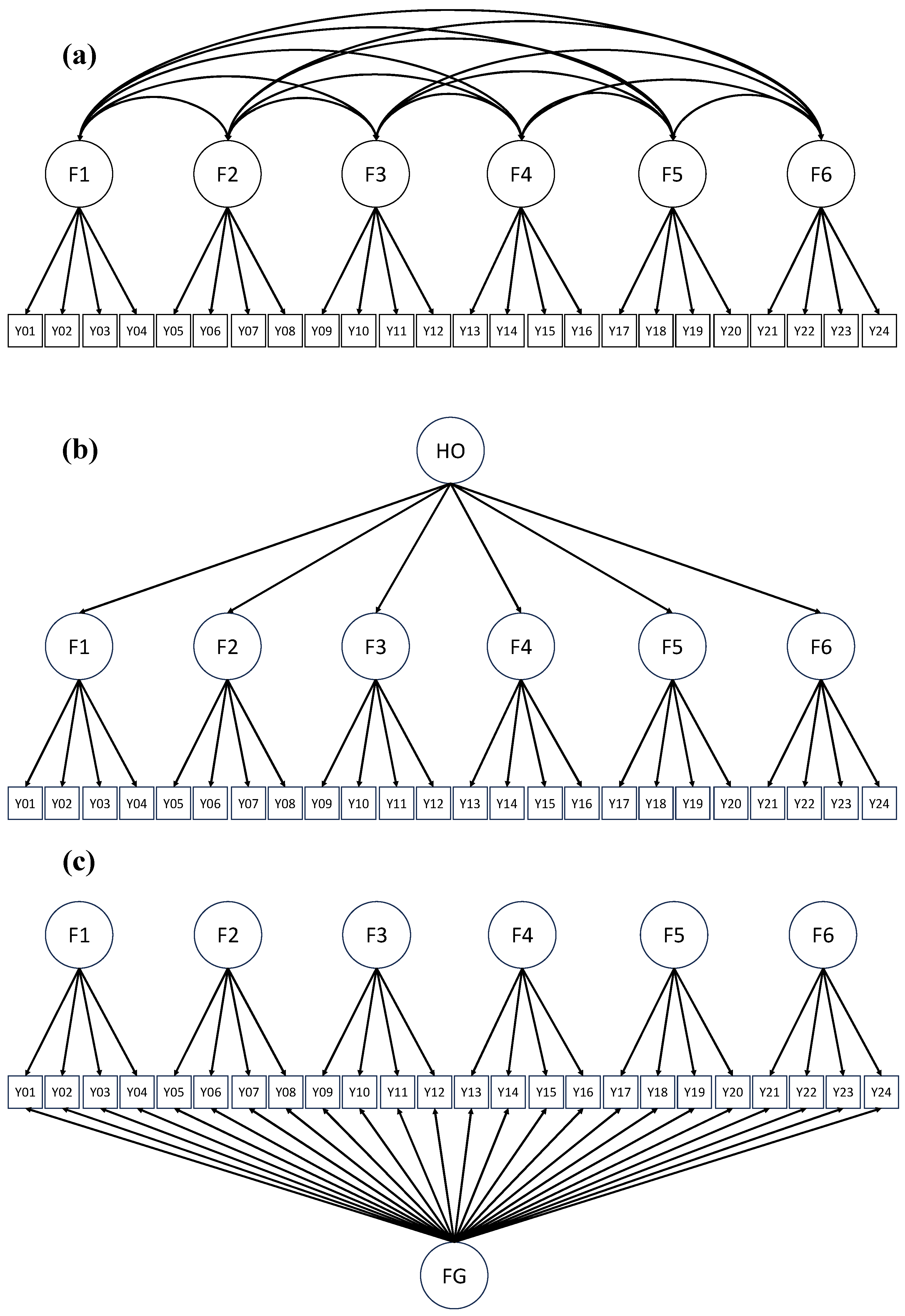
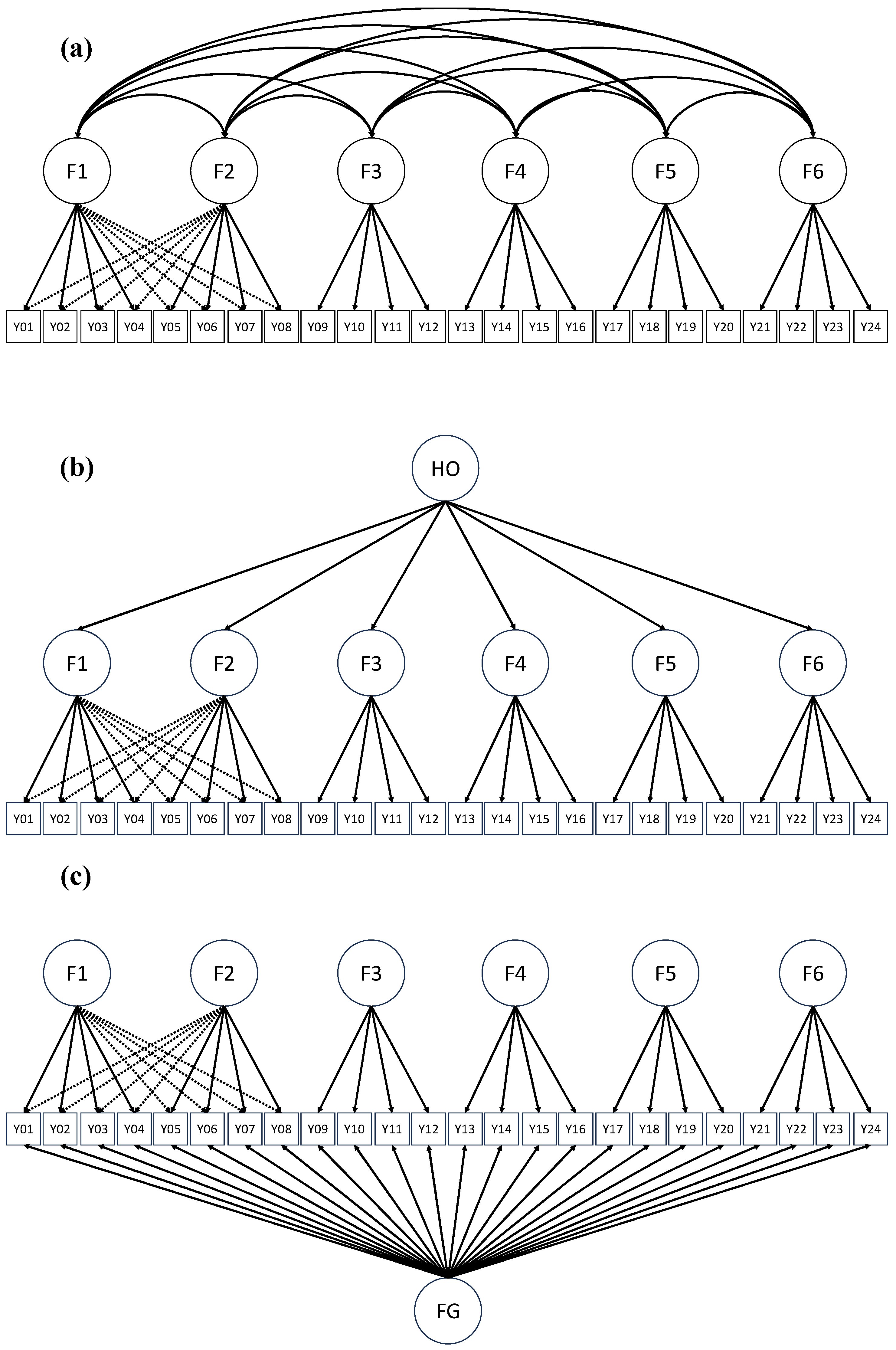

Disclaimer/Publisher’s Note: The statements, opinions and data contained in all publications are solely those of the individual author(s) and contributor(s) and not of MDPI and/or the editor(s). MDPI and/or the editor(s) disclaim responsibility for any injury to people or property resulting from any ideas, methods, instructions or products referred to in the content. |
© 2024 by the authors. Licensee MDPI, Basel, Switzerland. This article is an open access article distributed under the terms and conditions of the Creative Commons Attribution (CC BY) license (https://creativecommons.org/licenses/by/4.0/).