RMX/PIccc: An Extended Person–Item Map and a Unified IRT Output for eRm, psychotools, ltm, mirt, and TAM

Abstract

A constituting feature of item response models is that item and person parameters share a latent scale and are therefore comparable. The Person–Item Map is a useful graphical tool to visualize the alignment of the two parameter sets. However, the “classical” variant has some shortcomings, which are overcome by the new RMX package (Rasch models—eXtended). The package provides the RMX::plotPIccc() function, which creates an extended version of the classical PI Map, termed “PIccc”. It juxtaposes the person parameter distribution to various item-related functions, like category and item characteristic curves and category, item, and test information curves. The function supports many item response models and processes the return objects of five major R packages for IRT analysis. It returns the used parameters in a unified form, thus allowing for their further processing. The R package RMX is freely available at osf.io/n9c5r.

1. Introduction

In the seminal textbook of Fischer and Molenaar (1995; [1]), Erling B. Andersen [2]—“asked” about “What Georg Rasch Would Have Thought about this Book”—formulated:

But Rasch would have wondered about what happened to the use of graphs. And I think he would have been quite justified in this. Could it be that we have used computers in a wrong way? Since Rasch retired from active duty, have we emphasized the power of computers to do complicated calculations and solving complicated equations over the power of the computers to make nice and illustrative graphs?

([2]; p. 388)

In this vein, we want to introduce an extended version of the Person–Item Map (PI Map or Wright Map, cf. [3,4,5]). The PI Map is a graphical depiction of both item and person parameter estimates of an item response theory (IRT; [6]) model. It dates back to 1979 [7] and has gained popularity by its integration in the WinSteps software [8]. It juxtaposes the histogram of the person with the item parameter estimates based on the fact that they share a common latent scale. Wind and Hua [9] note that the PI Map should only be interpreted if the model fits (p. 14). However, the authors also carry out that plotting of non-fitting models might as well provide valuable hints for the reasons of the misfit.

In a test application, we gain most information about a test person when item difficulty and person ability align, but also obtain unbiased person parameter estimates with items “far away” from a respondee’s location on the latent scale (however, the standard error of the estimate increases with the distance). Analogously, we gain most information about an item when its difficulty aligns with the test persons’ abilities. The PI Map fosters the detection of such a mis-alignment. Debelak et al. (2022; [10] term this kind of analysis “sanity check” (p. 121). Refinements—like indicating the mean and standard deviation of either distribution—allow for “optimal targeting” (e.g., [3], p. 130). Boone et al. (2014; [3]), for example, show how PI Maps allow for detecting redundant items (referring to items with very similar difficulty parameters), which may prove useful if one is to develop a short form of a scale; or it shows “measurement gaps” (p. 129). Wind and Hua (2022; [9]) further point out that the spread of both the item and the person parameters also provides important information.

The WrightMap package [11] of R [12] is specialized in drawing PI Maps, supporting the output of the (non-R) program ConQuest [13]. Some of the major R packages for IRT also support the PI Map in one form or another, for example, eRm [14] with the plotPImap() function, psychotools [15] with the piplot() function (Figure 1), or TAM [16] with the IRT.WrightMap() wrapper to the WrightMap package.

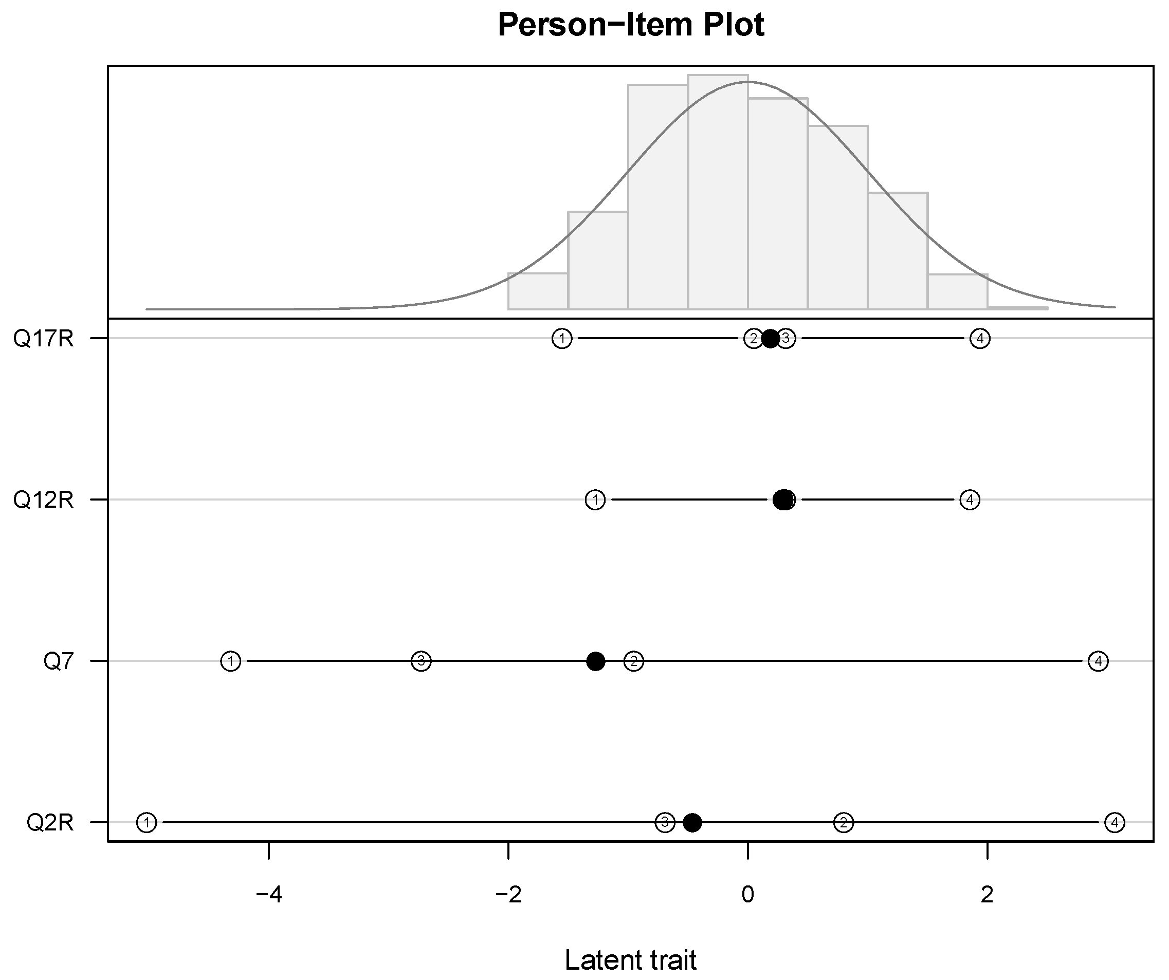
In this diagram, we find in the upper part a histogram of the person parameter estimates with the normal curve (using the mean and the standard deviation of the person parameter estimates) superimposed and in the lower part the threshold locations (numbered) along with their averages (bullets).

The diagram shows the results of a GPCM applied to the four items of the Agreeableness sub-scale of the Big Five inventory (see Section 3 for details regarding the data). The person parameter distribution is slightly right-skewed, ranging from $-2$ to +2. Compared to the majority of the persons’ locations, the items Q17R and Q12R appear optimally placed, with the first and the last threshold covering the range of the person parameter estimates. However, the two middle thresholds of these two items are very close to each other, indicating possible problems with the middle category. In contrast, we find a much larger range of the thresholds of items Q7 and Q2R, with both items’ first thresholds below $-4$. This could indicate that the lowest response categories were “easy” in a psychometric sense and therefore seldom used. Moreover, we find for the latter two items the middle thresholds’ positions exchanged, which might be due to problems with the middle category of the five-categorical response format.

Although this “classical” PI Map conveys important information regarding the locations of item and person parameters relative to each other, it withholds other important features of the items. For example:

−

Only the item difficulty/category threshold parameters are drawn, which is only partial information for models involving discrimination, guessing, or laziness parameters.

−

Although the threshold parameters are drawn for polytomous items, it is difficult to recognize which categories are likely to be chosen across the latent scale. Especially, the effects of threshold disorder are difficult to deduce.

−

Beyond item/threshold difficulty parameters, we may also learn a lot about our items in terms of information. The category and item information curves may tell us a lot if set into relation to the person parameter distribution.

−

Current implementations do not easily support flexibly arranging the items according to their characteristics (beyond difficulty) or, in the multidimensional case, dimensions.

−

Current implementations do not allow for varying the area proportions used for the person parameter histogram and the item parameter part. In Figure 1, it would be advantageous if we could increase the upper part at the expense of the item part.

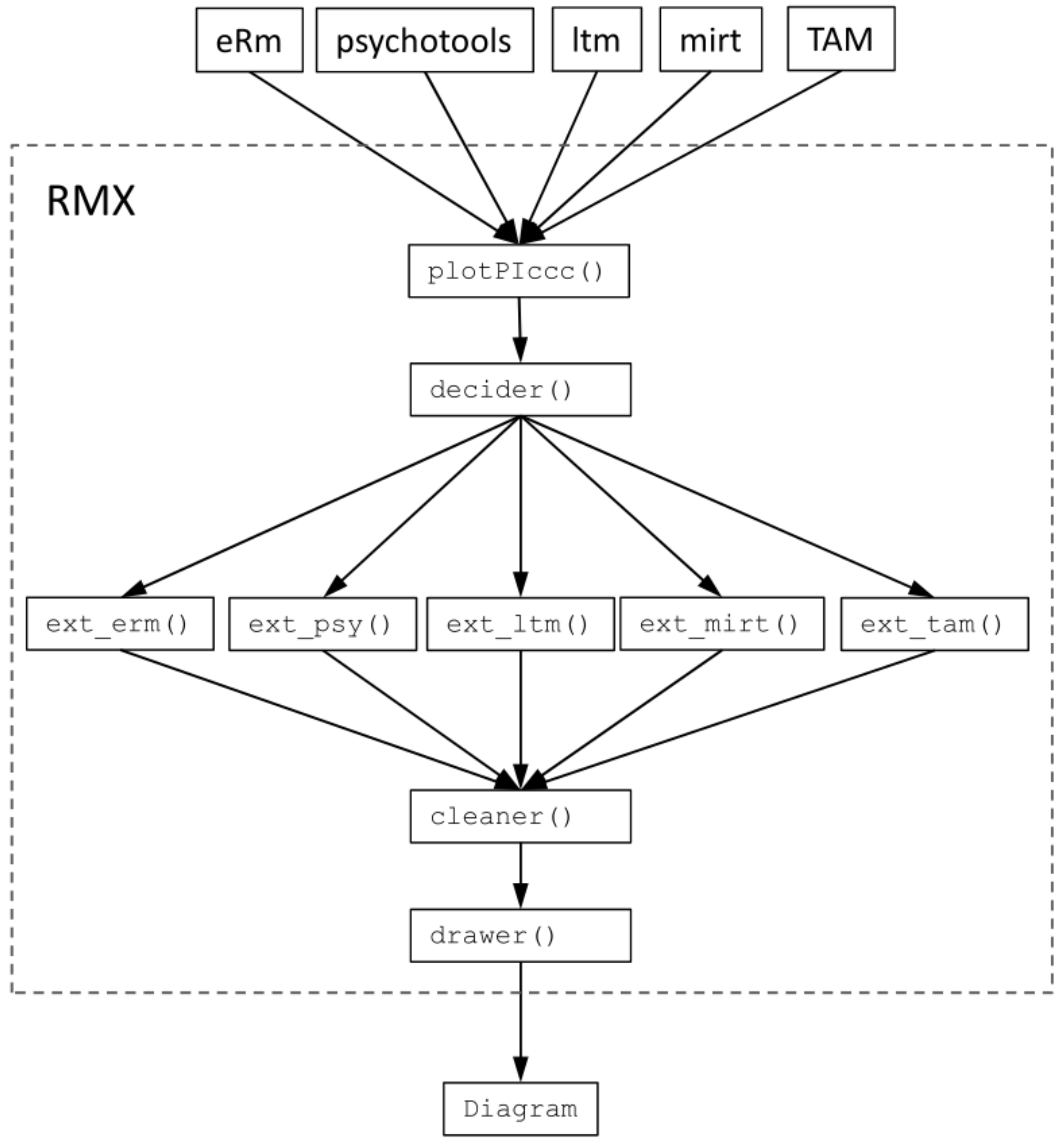
In this article, we want to introduce the R package RMX (Rasch models—eXtended). It currently provides the function RMX::plotPIccc(), which overcomes the restrictions of the “classical” PI Map in several respects. We term this modified diagram “PIccc” for it shows the Person–Item confrontation using category characteristic curves CCCs) and many other functions. Note that, although the package carries “Rasch” in its name, it does not only refer to the “Rasch Family of Models” (cf. [1]) but also to extensions covered by the term “Item Response Theory” (which is indicated by the “X”).

2. The RMX Package and the plotPIccc() Function

We start with a brief overview of the new package’s features and options, followed by a more technical description of how they were implemented.

2.1. Functionality Overview

The major innovation of a PIccc is to plot not only dots for difficulty or threshold parameters on the item side but also further model characteristics. Such an extension will prove especially useful for models involving parameters other than location only, i.e., non-Rasch models. These features are accessible via the type= argument, the options of which are listed in

Table 1. Options of the type= argument of RMX::plotPIccc().

Option	Curve Type
type="CCC"	the Category Characteristic Curve, a.k.a, Item Category Response Functions (ICRF), Category Response Functions (CRF), Operating Characteristic Curves (OCC), or Option Response Functions (ORF). The CCCs describe the probability of responding in a certain category given the location on the latent trait.
type="TCC"	the Threshold Characteristic Curve, a.k.a, Category Boundary Response Function (CBRF), Category Boundary Curves, Cumulative Probability Curves, or Boundary Characteristic Curves (cf. [6], p. 329). They describe “the probability of responding positively rather than negatively at a given boundary between two categories” (Ostini and Nering, 2006, [17], p. 9).
type="IIF"	the Item Information Function
type="CIF"	the Category Information Function, a.k.a Item Response Information Function (e.g., [18])
type="BIF"	both the CIF and the IIF (“Both Information Functions”)

.

Additionally, the function supports a classical=TRUE option, which draws the PI-Map in its traditional form (see Section 3).

The plotPIccc() function supports two modi, either

−

drawing one type of curve for a set of items (default); or

−

drawing several types for one item (by providing a vector of types).

In the former case, the items can optionally be selected with the isel= option (default: all items). For multidimensional models, the dsel= options allows item selection according to dimensions. The items may be sorted according to various item characteristics with the isort= option (see

Table 2. Options of the isort= argument of RMX::plotPIccc().

Sort Option	Sort Criterion	Applicable to
isort="mean"	the mean difficulty	all models
isort="median"	the median difficulty	all models
isort="var"	the variance of the thresholds	polytomous models
isort="min"	the minimum threshold	polytomous models
isort="max"	the maximum threshold	polytomous models
isort="range"	the threshold range	polytomous models
isort="disc"	the discrimination parameter	2/3/4PL, GPCM, GRM, and NRM
isort="guess"	the guessing parameter	3/4PL
isort="lazy"	the laziness parameter	4PL
isort="none"	keeping the original ordering	default

).

It is evident that options 3–6 (i.e., sorting by the variance, the minimum, the maximum, and range of thresholds) will have no effect for dichotomous models and neither will have isort="disc"/"guess"/"lazy" for the RM, the RSM, and the PCM. Note that selecting the isort="disc" option for the NRM will result in sorting by the average of the category discrimination parameters per item. Alternatively, the user may achieve any sorting by specifying the order of items in the isel= option. Additionally, the logical gsort= option switches for multidimensional models between sorting items within each dimension (FALSE) vs. globally (TRUE), i.e., across all dimensions.

Moreover, we can plot

−

the test information function (TIF) for the entire set of items (TIF=TRUE);

−

the TIF of the selected items (sTIF=TRUE);

−

the standard error (SE) for all items (SE=TRUE);

−

the SE of the selected items (sSE=TRUE); and

−

the kernel density estimate (dens=TRUE)

over the person parameter histogram (for the respective color options, see

Table 3. Color options of RMX::plotPIccc().

Option	Color of …
Person Parameter Area:
dimcol=	…the PP histogram(s)
dencol=	…the PP density line(s)
tifcol=	…the TIF line(s)
secol=	…the S.E. line(s)
Item Parameter Area:
funcol=	…the function lines, i.e., CCC, TCC, CIF; (see usedimcol=)
infcol=	…the IIF lines
discol=	…the disordered threshold indicator
bgcol=	…the background of the function plots
gridcol=	…the grid in the function plots
usedimcol=	Use dimension colors (dimcol=) for thresholds (classical=TRUE only; overrides funcol=)

).

The function also draws a category frequency barplot for the selected item(s). Many further options allow for fine-tuning the diagram, including several coloring options (see Table 3) or changing the proportions of the four plotting areas (funwprop= and funhprop=) and the range of the latent continuum to plot.

Users may choose a predefined color set for funcol=, which will also take precedence over the infcol= option. For multidimensional models, all options of the upper (person parameter) part of the PIccc accept color vectors. If the standard palette is used (default) and there are items with more than 8 categories, the colors will be recycled.

The package supports currently 10 different item response models from five packages (see

Table 4. Supported packages and models.

Model	eRm	Ltm	TAM	Mirt	Psychotools
Rasch Model (RM; [19])	√	√	√	√	√
2PL model [20]		√	√	√	√
3PL model [20]		√	√	√	√
4PL model [21,22]				√	√
Partial Credit Model (PCM; [23])	√	√	√	√	√
Rating Scale Model (RSM; [24])	√		√	√	√
Generalized Partial Credit Model (GPCM; [25])		√	√	√	√
Graded Response Model (GRM; [18])		√		√
Graded Rating Scale Model (GRSM; [26])				√
Nominal Response Model (NRM; [27,28,29])			(√) ${}^a$	√

${}^a$ Not yet supported by RMX.

for an overview of which package supports which model).

All models can be used in both the uni- and the multidimensional variant, as available in the supported packages (see Section 2.2 for details). Several of these possibilities will be demonstrated in Section 3.

The return object of RMX::plotPIccc() contains a list with the parameters used for plotting, thus fostering further processing, e.g., in a results table (see Section 3).

2.2. Some Technical Details

The RMX::plotPIccc() function automatically detects the package used for parameter estimation and unifies the various outputs.

2.2.1. Person Parameters

First of all, a PI Map requires both item and person parameters. IRT parameter estimation follows (except for JML, which is not considered here) a two-step strategy, estimating first the item parameters, which are then used for estimating the PP in a separate step. For that purpose, each package provides a specific routine (person.parameter() in eRm, personpar() in psychotools, factor.scores() in ltm, fscores() in mirt, and IRT.factor.scores.tam() or tam.wle() in TAM), some of which support several estimation variants. As the return objects of the model parameter estimation routines contain only the item parameters (except for TAM), RMX::plotPIccc() applies the appropriate PP estimation routine from the originating package with the default options. If a non-default PP estimation method is desired, one may use the pp= option and provide the return object of the respective package. For TAM, RMX::plotPIccc() uses the PPs provided already contained in the return object of the estimation routine.

One nifty feature might prove useful: if the user provides only the return object of the parameter estimating function of the originating package (which is required) and no person parameter object (i.e., pp=NULL), the RMX::plotPIccc() function estimates the person parameters internally. This may take a considerable amount of time for some models. Now, creating a PIccc likely takes several rounds with fine-tuning the graphical options until the optimal result is obtained. Letting the function recalculate the PPs each time can make the fine-tuning unnecessarily cumbersome. Therefore, RMX::plotPIccc() returns the PP object (as an attribute), which is automatically detected and could then be re-used in the pp= option:

  # first run:

    plotresult = RMX::plotPIccc(object, ... options ...)

  # subsequent runs:

    RMX::plotPIccc(object, pp=plotresult, ... better options ...)

This feature will save an enormous amount of time, especially when analyzing multidimensional models.

2.2.2. Model Formulations

There are two ways to formulate item response model equations, the “IRT” (or “slope-threshold”; ${\alpha }_j(\theta -{\beta }_j)$; cf. Garnier-Villarreal et al., 2021, [30]) and the “regression” (or “slope-intercept”; ${\alpha }_j\theta +d$; cf. de Ayala, 2022, [6], p. 18) variant, with eRm and psychotools returning the former and ltm, mirt, and TAM the latter (Note that mirt and TAM use cumulative intercepts in their outputs and eRm cumulative thresholds (for the latter, see [31])). The ltm routines (rasch(), ltm(), tpm(), gpcm(), and grm()) support an IRT.param=TRUE option in their function calls to switch between the two formulations (mirt also supports an IRTparams=TRUE in its coef() function and TAM has a set of “IRT.”-prefixed output functions, but these cannot be used here). Either way, RMX::plotPIccc() transforms all parameters into the slope threshold formulation, if necessary, and uses these values for plotting and in the return object.

2.2.3. Threshold Definitions

The category threshold parameters of divide-by-total models (following the taxonomy of Thissen and Steinberg, 1986, [32], p. 570) for ordered categories can be expressed the “Andrich/Masterian” or the “Thurstonian” way. The former indicates the CCC intersection locations of adjacent categories $j-1$ and j, i.e., $P(x=j-1)=P(x=j)$, and the latter denotes for each category c the location $\theta$ at which for response x holds that $P(x<j)=P(x\ge j)=0.5$ ([33]; notation adapted). The RMX::plotPIccc() function uses the Andrich/Masters formulation and transforms the input, if necessary. For type="CCC" or type="TCC", RMX::plotPIccc indicates threshold disordering with an asterisk (or the symbol set with disind=).

Two formulations have been developed for the NRM, which we term the “Bock” [27,29] and the “Thissen-Cai-Bock” (TCB; [34]) variant. They differ with respect to the slope/discrimination parameter $\alpha$: the Bock parametrization uses an item/category-specific slope parameter ${\alpha }_{ij}$ (for item i and category j, notation adapted), whereas the Thissen–Cai–Bock variant splits the slope into an item-specific parameter ${\alpha }_i^{*}$ and a category-specific scoring function $a_j$ (termed ak in mirt), the latter restricted to equality across items (notation adapted; see [34], Equation (3.32), for details). The advantage of the TCB variant is that it allows for formulating a multidimensional NRM with ${\alpha }_i^{*}$, which allows for an analogue interpretation as the loadings of a factor analysis. The RMX::plotPIccc() function uses the Bock parametrization [27], transforming the parameters following Thissen et al. [34], Equation (3.32), if necessary. Such a transformation is also applied for multidimensional models for we then obtain the category slope parameters for each item required for drawing. If the user requests type="TCC" for an NRM, the slopes of the lines are the category boundary discrimination ($CBD$) parameters

$$CBD={\alpha }_{ij}-{\alpha }_{i,j-1}$$

(1)

and their locations (i.e., points of inflection) b are the intersection points (using the category intercepts c and category slopes $\alpha$)

$$b_{i,j-1}=\frac{c_{i,j-1}-c_{ij}}{{\alpha }_{ij}-{\alpha }_{i,j-1}}=\frac{c_{i,j-1}-c_{ij}}{CBD}$$

(2)

([35], Equation (2); notation adapted).

For the GRM (a difference model in the taxonomy of Thissen and Steinberg, 1986, [32], p. 569), the program calculates and uses the differences in the cumulative probability formulation, i.e., the

$$P_{ij}=P_{ij}^{*}-P_{i,j+1}^{*}$$

(3)

(cf. Ostini and Nering, 2006, [17], p. 64, Equation  (1.2); notation adapted).

2.2.4. Multidimensional Models

The packages ltm, mirt, and TAM support multidimensional IRT models. The ltm routines allow for up to two exploratory dimensions, whereas mirt and TAM support an arbitrary number of dimensions in both a confirmatory and an exploratory modelling approach. RMX::plotPIccc() detects a multidimensional model automatically from the return object of the originating package. It plots (in the one type/several items mode) a diagram for each selected item and each selected dimension appearing in the model. Hence, an item appearing in more than one dimension (within-item multidimensionality) will be plotted more than once. The package supports both between- and within-item multidimensional compensatory models (The mirt package also supports non-compensatory models (sometimes referred to as partially compensatory (e.g., [36], Chapter 4), but only for dichotomous data. “[P]artially compensatory polytomous MIRT modes are yet to be developed.” ([37], p. 47)). It is important to note the following (dimensions indexed by $\ell =1\dots m$): we obtain each item’s parameters in the slope intercept (“regression”) formulation per dimension, i.e., a vector of length m of discrimination parameters $a_{i\ell }$ and the item’s intercept $d_i$. A slope threshold (“IRT”) formulation equivalent to the multidimensional slope for the 2PL (M2PL; cf. [36], Equation (4.5), p. 86) is the MDISC index

$$A_i=\sqrt{\sum _{\ell }{a}_{i\ell }^2}$$

(4)

(cf. [36], Equation (5.10), p. 118; notation adapted), which, in turn, allows for determining a multidimensional difficulty index MDIFF,

$$B_i=-\frac{d_i}{A_i}$$

(5)

(cf. [36], Equation (4.9), p. 90 and Equation (5.9), p. 117; notation adapted). The MDIFF index $B_i$ generalizes to the polytomous GRM by expansion to a vector across all thresholds per item. The MDISC index $A_i$ expresses the “steepest slope in a particular direction from the origin of the $\theta$-space.” ([37], p. 63; emphasis in the original). However, these indices are of limited value for the present purposes for two reasons:

First, they reduce each item’s dimension-specific slope $a_{i\ell }$ into one single number $A_i$, which would result in drawing the identical diagram for each dimension. One could, of course, enter MDIFF and MDISC in the model equations like in the uni-dimensional case and calculate that way the CCCs, TCCs, and the information functions. This yielded a diagram with several histograms for the person parameter estimates and one diagram per item based on the multidimensional indices.

Second, there is a more fundamental shortcoming in that MDIFF and MDISC are only defined for dichotomous models and the GRM (Note that mirt already calculates MDISC and MDIFF for multidimensional dichotomous models and the GRM. Other function calls stop with Error in MDIFF(…):Item 1 is not of class "graded" or "dich"), thus limiting the support of RMX to these models. Multidimensional PCMs, RSMs, and GPCMs could not be drawn that way.

We, therefore, chose a slightly different approach: Because we seek each item’s characteristics within each dimension separately (i.e., the “marginal” parameters, in an ANOVA-like notion), we apply an adaptation of the uni-dimensional transformation of the “regression” into the “IRT” formulation, i.e.,

$$b_{i\ell }=-\frac{d_i}{a_{i\ell }}$$

(6)

(with $b_{i\ell }$ denoting the “marginal” item difficulty parameter of item i in dimension ℓ) for all multidimensional models originating from ltm, mirt, and TAM. The rationale for this approach builds ultimately on the Pythagorean theorem, as visualized in [37], p. 62, Figure 5.6: We use the cathetes (i.e., $a_{i\ell }$) rather than the hypothenuse (i.e., $A_i$) in the denominator. A drawback of Equation (6) is that possible correlations of the latent dimensions are not taken into consideration. This seemed an acceptable solution insofar as the program focuses on the items’ specific properties rather than their multidimensional interpretation. For a correct interpretation of the plots drawn with RMX::plotPIccc(), we have to keep in mind that the parameters used here “give the relative difficulty of the item related to the corresponding coordinate dimension” ([36], p. 89).

2.2.5. Information Functions

The item information functions for all divide-by-total models for ordered categories are calculated according to Masters and Evans (1986; [38], p. 362, Equation (3)), those of the GRM according to Samejima (1968; [18], p. 60, Equation (6-6)), and those of the NRM according to Bock (1970; [27], p. 44, Equations (24) and (25)). The category information functions are obtained according to Muraki (1993; [39], p. 354, Equation (13)).

In contrast to the probability-based functions CCC and TCC, the information functions do not have an interpretable maximum. The RMX::plotPIccc() function provides, therefore, the infomax= option, which takes either the keywords infomax="auto" and infomax="equal" or a numeric value indicating the maximum value to plot. With "auto", each diagram is zoomed to its individual maximum, whereas "equal" uses a common scale for all visible information diagrams (i.e., the common maximum across items in the multiple items/one function mode or the common maximum across the chosen information functions in the one-item/multiple-functions mode).

2.2.6. The Internal Structure and the Return Object

The various features are implemented in a workflow shown in Figure 2. Currently, RMX exports only the RMX::plotPIccc() function, but users may directly call the five extractor functions (i.e., ext_erm(), ext_psy(), ext_ltm(), ext_mirt(), and ext_tam()) using the triple colon (:::) operator. Each of them expects the return object of the originating package and determines the dimensionality of the model, extracts the item parameters (per dimension, if applicable), calculates/extracts the person parameters (also per dimension, if applicable), counts the response frequencies of all categories of each item, and returns a list. Note that all item parameters will be returned in the slope threshold (“IRT”) formulation. The cleaner() function selects the required items and (if admissible) dimensions (isel=, dsel=) and sorts them (isort=). The return object of the cleaner() is then used by the drawer().

The return object is a list containing one element per latent dimension each containing all selected item parameters, i.e.,

−

matrices with the location estimates in the slope-threshold formulation;

−

discrimination, guessing, and laziness parameters;

−

a vector indicating each item’s model (as mirt allows for varying models across items);

−

a vector of length n with the person parameter estimates of this dimension;

−

vectors of length $n^{*}=1001$ (tmin to tmax) with TIF, sTIF, SE, and sSE; and

−

matrices ($n^{*}\times k$) with CCCs, TCCs, CIFs, and IIFs,

with n for the sample size, $n^{*}$ for the grid along the horizontal axis used for drawing the lines, and k for the number of items.

Next to the dimension elements, level 1 of the return object also contains a list of length k with each item’s category response frequencies table and finally the sort vector. Additionally, the return object carries two attributes, a string with the originating package and model and the complete result object from the person parameter estimation (required for the time-saving feature described above). With these detailed results, the RMX::plotPIccc() function may also serve as a tool for further processing the results of an analysis (e.g., as a table; see the last listing 4), even if no diagram is required (option plot=FALSE).

3. Worked Examples

For demonstrating some of the capabilities of RMX::plotPIccc(), we use the example dataset big5 delivered with the RMX package. Mimicking a students’ survey, it comprises 21 items covering the Big Five (i.e., Openness, Conscientiousness, Extraversion, Agreeableness, and Neuroticism; [40]) and 1076 simulated respondents. The response format of all items was Likert-type, with the categories “very inapplicable”, “rather inapplicable”, “neither-nor”, “rather true”, and “very true” (translated from the German original).

The first example (Listing 1) shows the diagram of a GPCM evaluated with psychotools using the default options of RMX::plotPIccc():

Listing 1. Example of a GPCM with psychotools using the Agreeableness items.

library(RMX)

library(psychotools)

mod1 = psychotools::gpcmodel(big5[,c(2,7,12,17)])

RMX::plotPIccc(mod1)

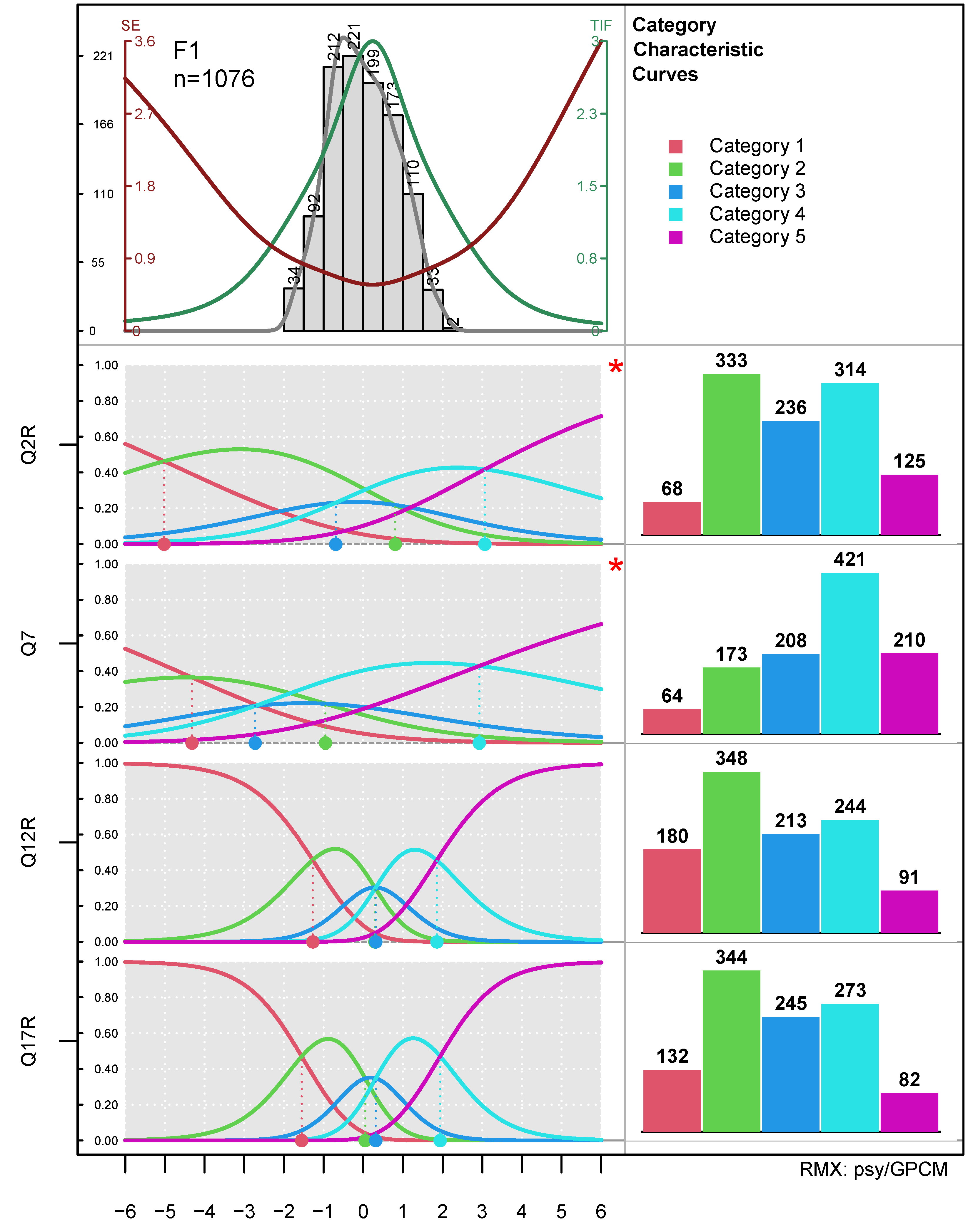
In Figure 3, we find four areas of output: the top left segment shows the person parameter histogram, here with the default option pplab="abs" for absolute frequencies (alternatively pplab="rel" for percentages or pplab="dens" for the kernel density estimates). The green line is the test information function (TIF) and the red line the standard error (SE). Additionally, if only a subset of items is used, dashed lines indicate the TIF and the SE of the selected items in the respective colors. The top right segment holds the legend for the one-function/several-items mode and the category frequency barchart for the one-item/several-functions mode (see Figure 4 for the latter). The lower left segment shows the item-related functions, i.e., the CCCs by default in the one-function/several-items case or the selected functions in the one-item/several-functions case. The lower right segment shows the category response frequency barcharts of each item in the one-function/several-items mode and the legend of the respective function in the one-item/several-functions mode. The upper : lower and left : right proportions can be adapted with the funhprop= and the funwprop= option, each taking decimal values between zero and one. Values of zero or one for either option will switch on/off the entire regions so that each of the four segments can be drawn alone.

The diagram in Figure 3 is based on the same data as used in Figure 1. Note that the items are ordered from top to bottom (i.e., reversed compared to Figure 1), thus following the ordering of the items. The CCCs of this diagram immediately show that the spread of the thresholds of items Q2R and Q7 (observed in Figure 1) is due to the low discrimination of these two items (${\alpha }_{\mathrm{Q}2\mathrm{R}}=0.35$ and ${\alpha }_{\mathrm{Q}7}=0.26$). Again, we find thresholds 2 and 3 reversed (indicated by asterisks), and we can confirm the suspicion from Figure 1 that the lowest categories of these two items were barely used. From the CCCs, we also see that the middle category was at no point of the latent continuum the most attractive one. Additionally, we see that the TIF of this sub-scale has a strong peak, which went undetected in the classical variant of the PI Map.

The next example demonstrates the one-item/multiple-functions mode. We estimate a GPCM for the Neuroticism subscale of the Big Five example dataset (i.e., items 4, 9, 14, and 19; Listing 2).

Listing 2. Example of a GPCM using TAM.

library(TAM)

mod2a = TAM::tam.mml(    big5[,c(4,9,14,19)],verbose=FALSE) # Neuroticism

mod2b = TAM::tam.mml.2pl(big5[,c(4,9,14,19)],verbose=FALSE)

RMX::plotPIccc(mod2a,type=c("CCC","TCC","BIF"),isel=2,infomax=1.05)

RMX::plotPIccc(mod2b,type=c("CCC","TCC","BIF"),isel=2,infomax=1.05)

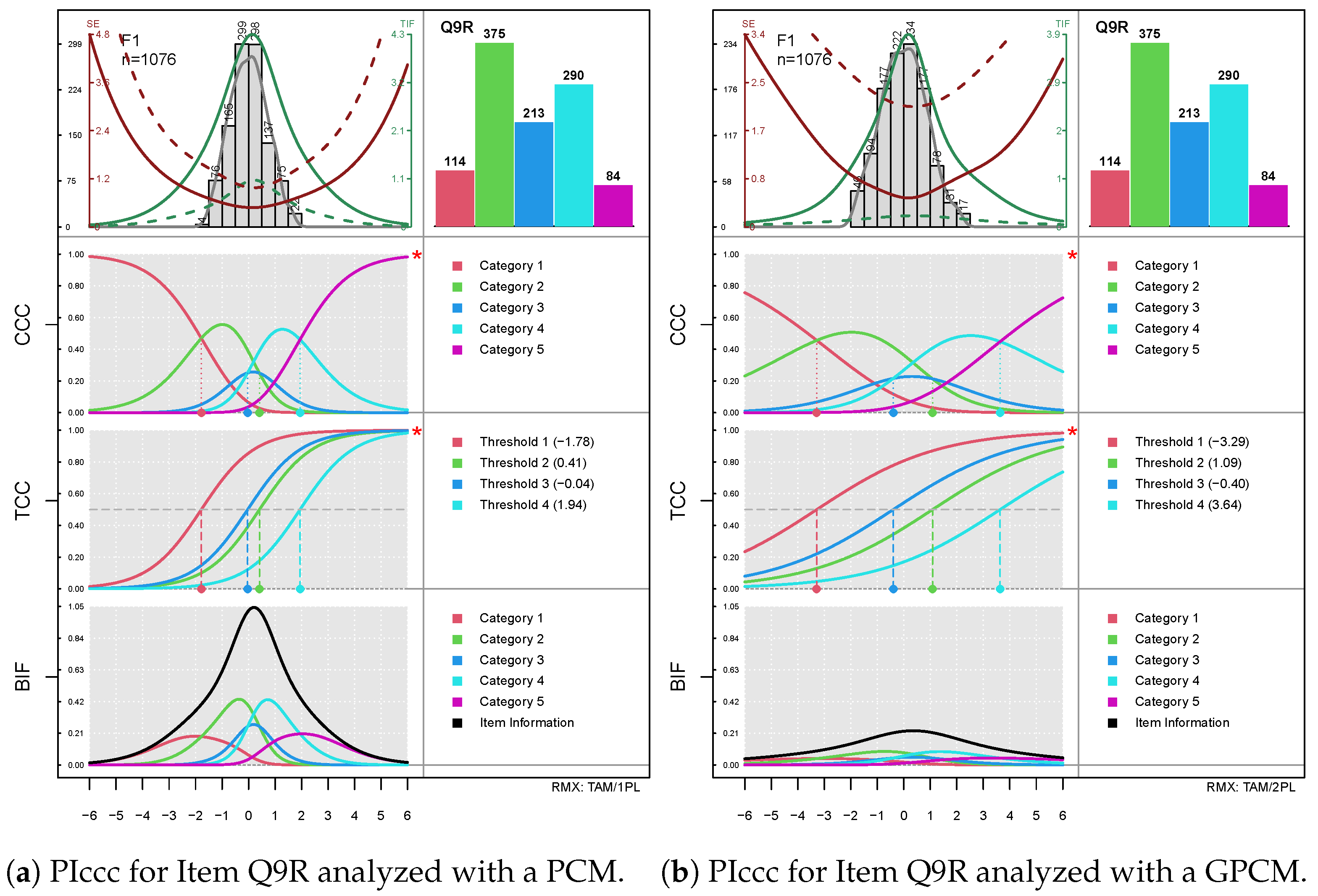
Figure 4 shows the output of the multiple-type diagram for item Q9R of the Neuroticism subscale. In this mode, the barchart with the category frequencies is shifted to the top and the legends are now placed to the right of each diagram. In the top left area, we now see not only the TIF and SE lines (solid) but also the respective dashed lines for the selected item, as mentioned above. The latter allow for comparing the item’s contribution to the test information. Note that the arrangement of the three functions follows the ordering in the type= option.

By comparing the two diagrams, we see clearly the differences in the item’s discrimination parameter, which is 1 for the PCM and ${\alpha }_{\mathrm{Q}9\mathrm{R}}=0.436$ for the GPCM. Accordingly, the CCCs and TCCs in the right diagram (Figure 4b) are clearly flatter than those in the left one (Figure 4a). Interestingly, the maximum item information also differs remarkably (1.04 for the PCM vs. 0.23 for the GPCM; we used the infomax= option to equalize the scales of the two information functions). Here, we see clearly that the improvement in fit due to varying slopes comes at the cost of information. The item shows a threshold disordering for both models, which is indicated by the red asterisks. Thus, the weaknesses of the item become visible at a glance. Moreover, the comparison of the sSE curves of this item (dotted red lines) shows that the GPCM-based standard errors are remarkably larger than those based on the PCM, which is a result of the lower discrimination parameter of this item.

Next, we demonstrate the output of a multidimensional diagram using the classical form (Listing 3).

Listing 3. Example of a multidimensional GPCM using mirt and the Big Five example dataset.

big5mod = "O = 5,10,15,20,21

C = 3,8,13,18

E = 1,6,11,16

A = 2,7,12,17

N = 4,9,14,19

COV=O*C*E*A*N"

big5res = mirt::mirt(big5,big5mod,itemtype="gpcm",method="MHRM")

big5est = RMX::plotPIccc(big5res,classical=TRUE,  lmar=3,  ylas=2,

funhprop=0.6,dencol=NA,usedimcol=TRUE,

dimcol=c("#bef7ff", "#a0dcff", "#82c2ff", "#63a7ff", "#458cff"),

tifcol=grey(0.6), secol="dodgerblue4")

Figure 5 shows the output of Listing 3.

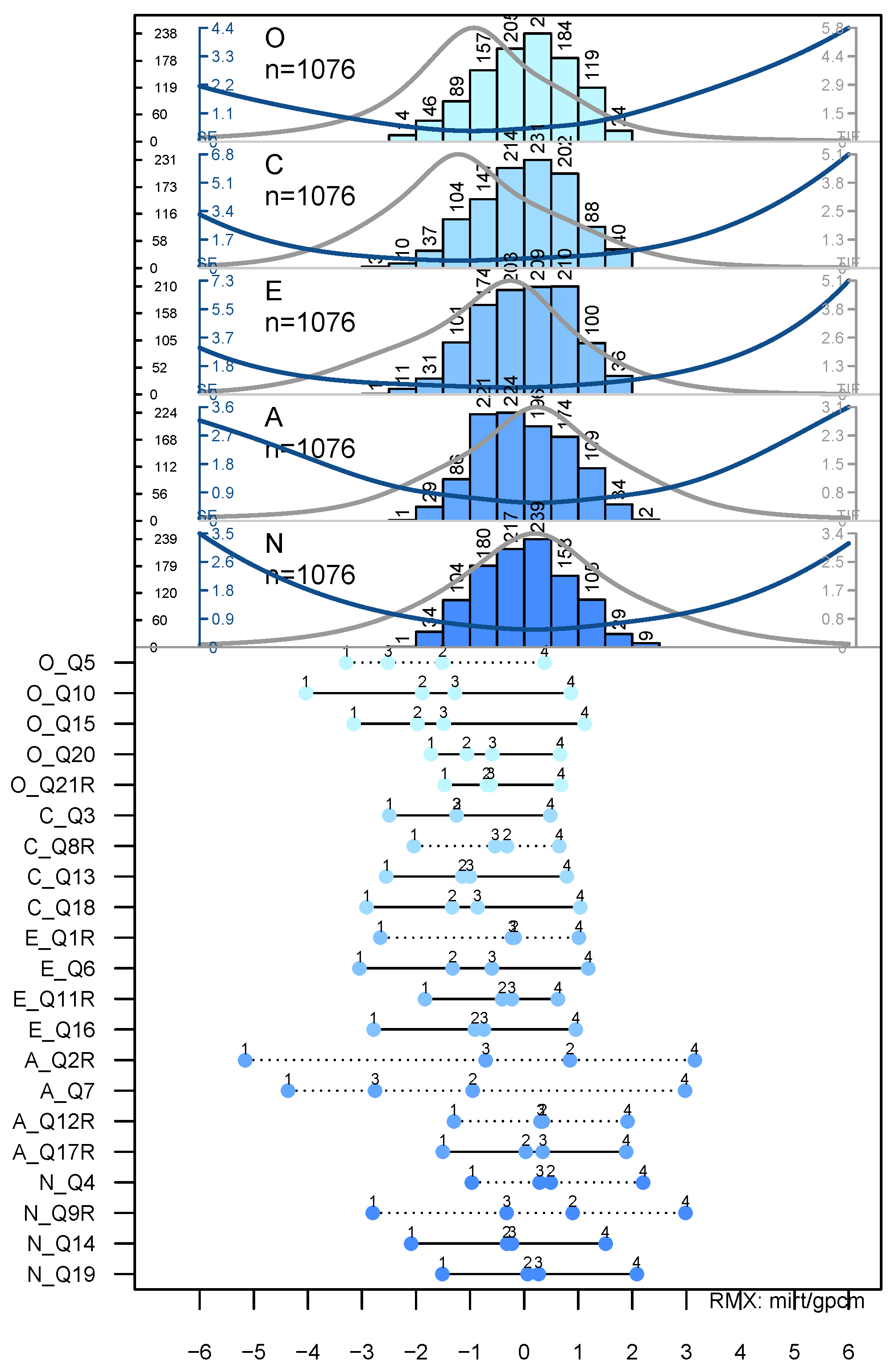
The lmar=3 and ylas=2 options allowed for printing the item labels, which have been automatically extended by the dimension labels. With the option usedimcol=TRUE, we colored the items’ dots according to their respective latent dimension. Note further that, in the classical=TRUE variant, threshold disordering is indicated with dotted lines.

From Figure 5, we learn that the items’ thresholds exceed the range of the person parameters and that eight items show threshold disordering. Another interesting feature becomes visible here: the combined depiction of the person parameter histogram and the TIF allows for examining whether the instrument (here, sub-scale) measures best where the respondents are located. Such a comparison could be useful for clinical applications, for example, to check whether the instrument works better for inpatients or for screening purposes in the general population.

For publishing, one could redirect the output to a suitably formatted file with the pdf() or png() function of R (the former yielding scalable images). That way, the user may choose the optimal window proportions (width=, height=), which is the reason why the plot opens by default in an external window (RStudio/posit [41] users may set extwin=FALSE to use the internal graphics viewer). Internally, RMX::plotPIccc() uses for the external graphics window the generic dev.new() function of R with the noRStudioGD=TRUE option set. The extwin=FALSE option is also required if one uses RMX::plotPIccc() for compiling a markdown output, which is readily supported by RStudio/posit. Additionally, the option resetpar= (default: TRUE) controls, whether the graphic parameters (set with par()) are restored after the drawing has finished. Setting to FALSE allows for further refinements of the diagram (e.g., additional text, arrows, etc.).

The RMX::plotPIccc() function returns (invisibly) a list with all values used for plotting, which may be useful for publishing the results. Listing 4 shows, exemplarily, how to build a table for LATEX using the xtable package [42] of R using the return object big5est from Listing 3:

Listing 4. Processing the return object of the analysis of Listing 3.

xtable::xtable(big5est$N$thresholds)

\begin{table}[H]

\centering

\begin{tabular}{rrrrr}\hline

&   Q4 &    Q9R &    Q14 &  Q19 \\\hline

1 &  -0.97 &  -2.79 &  -2.09 &  -1.51 \\

2 &  0.49 &  0.90 &  -0.32 &  0.07 \\

3 &  0.29 &  -0.32 &  -0.22 &  0.27 \\

4 &  2.20 &  2.99 &  1.51 &  2.09 \\\hline

\end{tabular}

\end{table}

This code yields the following

Table 5. Parameter table built with xtable::xtable in its raw form.

	Q4	Q9R	Q14	Q19
1	−0.97	−2.79	−2.09	−1.51
2	0.49	0.90	−0.32	0.07
3	0.29	−0.32	−0.22	0.27
4	2.20	2.99	1.51	2.09

(kept in its original format, improvements ad lib):

Non-LATEX users may as well use different packages (e.g., knitr [43,44], pandoc [45], sjplot [46], R2wd [47], etc.) to transform the output into a form compatible with one’s favorite text processing software.

4. Discussion

In this article, we introduced the RMX package, which provides the PIccc, an extended Person–Item Map. In addition to plotting the estimated difficulty and threshold parameters, it also supports a set of item-related functions, like the CCC, the TCC, and various information functions. This allows for a more efficient assessment of the items’ functioning and the alignment of person and item parameters.

Aside from the multi-purpose PIccc, the RMX::plotPIccc() function may also be used to draw simple diagrams of a single item’s CCC, TCC, CIF, IIF, or the category frequencies barplot only by using the isel=, funhprop=, and funwprop= options. Thus, the package offers enormous flexibility by covering functionality, which may require more programming effort in the other packages, if supported at all. It further improves some of the other packages’ functions in terms of graphical options.

In contrast to the classical PI Map, the new PIccc diagram works best with only a few items (except, of course, for classical=TRUE). This may require to split items across multiple diagrams, e.g., according to sub-scales or other substantive criteria. However, the alternative (so far) was to plot each, say, CCC separately per item (possibly gathering them in a plot matrix), which makes comparisons more difficult, not to mention the limited comparability to the person parameter distribution. Therefore, the presented solution seems to be a major step forward in this respect.

4.1. Threshold (Dis)Ordering in the NRM

When analyzing items with the NRM, threshold disordering is indicated by the CBDs rather than the intersection points like in the (G)PCM ([48], but opposed by [49]). This is exactly what the PIccc diagram draws with the option type="TCC", thus allowing for easily detecting threshold disordering. Importantly, the type="CCC" will not allow for detecting threshold disordering for the NRM as a category could indeed lack a range on the latent continuum, along which it has a larger probability to be chosen than any other category, although thresholds are ordered. This is in contrast to the (G)PCM, where threshold disordering is always associated with categories “vanishing” behind others. To our knowledge, RMX::plotPIccc() is the first program directly implementing a graphical disorder detection feature for the NRM.

4.2. Sorting Items in the NRM

The RMX::plotPIccc() function allows for sorting polytomous items according to several criteria, including the discrimination parameters. For the NRM, this is not possible in a straightforward manner because it estimates a discrimination parameter for each category of an item. Therefore, we use the mean of the discrimination parameters per item for sorting. Alternatively, sorting could also be achieved by using the item-wise (i.e., single-indexed) discrimination parameter as defined by Thissen et al. (2010; [34]), which is planned for a further release of RMX.

4.3. Estimating the Person Parameters

Regarding the person parameters, we have to distinguish the CML- and the MML-based methods ([50]), with eRm and psychotools supporting the former and ltm, mirt, and TAM the latter. In the CML context, no person parameter estimates can be obtained for perfect and zero scores as they tend to add or subtract infinity, respectively (The same applies to the item parameter estimation; i.e., items with zero or perfect scores will also require special treatment, but this is already handled in the originating packages). However, making certain additional assumptions allows for generating surrogate values. The eRm package applies a spline interpolation to the score-$\theta$ function and extrapolates estimates for zero and maximum possible score using the extrapolate=TRUE option in the coef() function. In contrast, the psychotools package will just return NA for respondents with zero or perfect scores.

We encounter a similar situation for datasets containing missing values. The eRm routines evaluate each missing pattern separately and return a vector with the respective estimates for all respondents. In contrast, psychotools also return NA if a response vector contains missing values. Therefore, the N= shown in the person parameter distribution area may differ from the actual sample size if the originating package was psychotools. In contrast, the MML-based packages can handle zero and perfect scores.

5. Conclusions and Outlook

The RMX package may be of great help not only for test developers, who can easily recognize relevant information about the items’ functioning, but also in an educational context to visualize the various aspects of all IRT models and packages covered, i.e., eRm, psychotools, ltm, mirt, and TAM. To highlight the innovations of RMX::plotPIccc(), consider the partial TIF and SE of selected items, flexible area proportions, multiple functions for an item, unified output using the slope difficulty formulation for all models, flexible selection of items and/or dimensions, TCC for the NRM, allowing for visually detecting threshold disordering, many graphical options to fine-tune the diagram, and support of all major IRT packages of R and many IRT models (as shown in Table 4). We further hope that the easy availability of the many type options for analysis will pass attention to more diverse item analyses involving the CCCs, the TCC, and the various information functions. We therefore think that the RMX package constitutes a considerable step forward regarding graphical item analysis in the sense of Andersen/Rasch.

The package is freely available at https://osf.io/n9c5r/ (accessed on 28 August 2023) where users will also find a gallery demonstrating the capabilities of RMX::plotPIccc(). The current version has been developed with

−

eRm 1.0-2 (https://cran.r-project.org/package=eRm; accessed on 28 August 2023),

−

ltm 1.2-0 (https://cran.r-project.org/package=ltm; accessed on 28 August 2023),

−

psychotools 0.7-3 (https://cran.r-project.org/package=psychotools; accessed on 28 August 2023),

−

mirt 1.40 (https://cran.r-project.org/package=mirt; accessed on 28 August 2023), and

−

TAM 4.1-4 (https://cran.r-project.org/package=TAM; accessed on 28 August 2023).

Further diagrams are currently under construction and will be added to future versions of the RMX package, which will then be made available on CRAN.

References

1. Fischer, G.H.; Molenaar, I.W. (Eds.) Rasch Models. Foundations, Recent Developments, and Applications; Springer: Berlin/Heidelberg, Germany, 1995. [Google Scholar]
2. Andersen, E.B. What Georg Rasch Would Have Thought about this Book. In Rasch Models. Foundations, Recent Developments, and Applications; Fischer, G.H., Molenaar, I.W., Eds.; Springer: New York, NY, USA, 1995; pp. 383–390. [Google Scholar] [CrossRef]
3. Boone, W.J.; Staver, J.R.; Yale, M.S. Rasch Analysis in the Human Sciences; Springer: Dordrecht, The Netherlands, 2014. [Google Scholar] [CrossRef]
4. Wilson, M. Constructing Measures. An Item Response Modeling Approach; Taylor & Francis; Psychology Press: New York, NY, USA, 2005. [Google Scholar]
5. Wilson, M. Some Notes on the Term: “Wright Map”. Rasch Meas. Trans. 2011, 25, 1331. Available online: https://rasch.org/rmt/rmt253b.htm (accessed on 28 August 2023).
6. De Ayala, R.J. The Theory and Practice of Item Response Theory, 2nd ed.; The Guilford Press: New York, NY, USA, 2022. [Google Scholar]
7. Wright, B.D.; Stone, M.H. Best Test Design; Mesa Press: Chicago, IL, USA, 1979. [Google Scholar]
8. Linacre, J.M. Winsteps® Rasch Measurement Computer Program. Available online: https://Winsteps.com (accessed on 28 August 2023).
9. Wind, S.; Hua, C. Rasch Measurement Theory Analysis in R; Chapman and Hall; CRC: New York, NY, USA, 2022. [Google Scholar] [CrossRef]
10. Debelak, R.; Strobl, C.; Zeigenfuse, M.D. An Introduction to the Rasch Model with Examples in R; CRC/Chapman & Hall: Boca Raton, FL, USA, 2022. [Google Scholar] [CrossRef]
11. Irribarra, D.T.; Freund, R. Wright Map: IRT Item-Person Map with Conquest Integration. 2014. Available online: https://github.com/david-ti/wrightmap (accessed on 28 August 2023).
12. Team, R.C. R: A Language and Environment for Statistical Computing; R Foundation for Statistical Computing: Vienna, Austria, 2023. [Google Scholar]
13. Adams, R.J.; Wu, M.L.; Cloney, D.; Berezner, A.; Wilson, M.R. ACER ConQuest: Generalised Item Response Modelling Software. 2020. [Computer Program] Australian Council for Educational Research. Available online: https://www.acer.org/au/conquest (accessed on 28 August 2023).
14. Mair, P.; Hatzinger, R.; Maier, M.J. eRm: Extended Rasch Modeling. 2020. 1.0-2. Available online: https://CRAN.R-project.org/package=eRm (accessed on 28 August 2023).
15. Zeileis, A.; Strobl, C.; Wickelmaier, F.; Komboz, B.; Kopf, J.; Schneider, L.; Debelak, R. Psychotools: Infrastructure for Psychometric Modeling. 2021. R Package Version 0.7-0. Available online: https://CRAN.R-project.org/package=psychotools (accessed on 28 August 2023).
16. Robitzsch, A.; Kiefer, T.; Wu, M. TAM: Test Analysis Modules, R Package Version 3.4-26; R Foundation for Statistical Computing: Vienna, Austria, 2020; Available online: https://CRAN.R-project.org/package=TAM (accessed on 28 August 2023).
17. Ostini, R.; Nering, M.L. Polytomous Item Response Theory Models; Sage: Thousand Oaks, CA, USA, 2006. [Google Scholar]
18. Samejima, F. Estimation of Latent Ability Using a Response Pattern of Graded Scores. Educ. Test. Serv. Res. Bull. 1968, RB-68-2, 1–169. [Google Scholar]
19. Rasch, G. Probabilistic Models for Some Intelligence and Attainment Tests; Danmarks Pædagogiske Institut: Copenhagen, Denmark, 1960. [Google Scholar]
20. Birnbaum, A. Some Latent Trait Models and Their Use in Inferring an Examinee’s Ability. In Statistical Theories of Mental Test Scores; Lord, F.M., Novick, M.R., Eds.; Addison-Wesley: Reading, MA, USA, 1968; Chapter 17–20; pp. 395–479. [Google Scholar]
21. Barton, M.A.; Lord, F.M. An Upper Asymptote for the Three-Parameter Logistic Item-Response Model; Educational Testing Service Research Report Series [RR-81-20]; ETS: Princeton, NJ, USA, 1981. [Google Scholar] [CrossRef]
22. Loken, E.; Rulison, K.L. Estimation of a four-parameter item response theory model. Br. J. Math. Stat. Psychol. 2010, 63, 509–525. [Google Scholar] [CrossRef] [PubMed]
23. Masters, G.N. A Rasch Model for Partial Credit Scoring. Psychometrika 1982, 47, 149–174. [Google Scholar] [CrossRef]
24. Andrich, D. A rating formulation for ordered response categories. Psychometrika 1978, 43, 561–573. [Google Scholar] [CrossRef]
25. Muraki, E. A Generalized Partial Credit Model: Application of an EM Algorithm. Appl. Psychol. Meas. 1992, 16, 159–176. [Google Scholar] [CrossRef]
26. Muraki, E. Fitting a Polytomous Item Response Model to Likert-Type Data. Appl. Psychol. Meas. 1990, 14, 59–71. [Google Scholar] [CrossRef]
27. Bock, R.D. Estimating item parameters and latent ability when responses are scored in two or more nominal categories. Psychometrika 1970, 37, 29–51. [Google Scholar] [CrossRef]
28. Thissen, D.; Steinberg, L. A Response Model for Multiple Choice Items. Psychometrika 1984, 49, 501–519. [Google Scholar] [CrossRef]
29. Thissen, D.; Steinberg, L. A Response Model for Multiple-Choice Items. In Handbook of Modern Item Response Theory; van der Linden, W.J., Hambleton, R.K., Eds.; Springer: New York, NY, USA, 1997; pp. 51–65. [Google Scholar]
30. Garnier-Villarreal, M.; Merkle, E.C.; Magnus, B.E. Between-Item Multidimensional IRT: How Far Can the Estimation Methods Go? Psych 2021, 3, 404–421. [Google Scholar] [CrossRef]
31. Alexandrowicz, R.W. GMX: Extended Graphical Model Checks. A Versatile Replacement of the plotGOF() Function of eRm. Psychol. Test Assess. Model. 2022, 64, 215–225. [Google Scholar]
32. Thissen, D.; Steinberg, L. A Taxonomy of Item Response Models. Psychometrika 1986, 51, 567–577. [Google Scholar] [CrossRef]
33. Wilson, M. Dichotomizing Rating Scales and Rasch-Thurstone Thresholds. Rasch Meas. Trans. 2009, 23, 1228. Available online: https://www.rasch.org/rmt/rmt233e.htm (accessed on 28 August 2023).
34. Thissen, D.; Cai, L.; Bock, R.D. The Nominal Categories Item Response Model. In Handbook of Polytomous Item Response Theory Models; Nering, M.L., Ostini, R., Eds.; Taylor & Francis: New York, NY, USA, 2010; pp. 43–75. [Google Scholar]
35. De Ayala, R.J.; Sava-Bolesta, M. Item Parameter Recovery for the Nominal Response Model. Appl. Psychol. Meas. 1999, 23, 3–19. [Google Scholar] [CrossRef]
36. Reckase, M.D. Multidimensional Item Response Theory; Springer: New York, NY, USA, 2009. [Google Scholar] [CrossRef]
37. Bonifay, W. Multidimensional Item Response Theory; Sage: Thousand Oaks, CA, USA, 2020. [Google Scholar] [CrossRef]
38. Masters, G.N.; Evans, J. Banking Non-Dichotomously Scored Items. Appl. Psychol. Meas. 1986, 10, 335–367. [Google Scholar]
39. Muraki, E. Information Functions of the Generalized Partial Credit Model. Appl. Psychol. Meas. 1993, 17, 351–363. [Google Scholar] [CrossRef]
40. Rammstedt, B.; John, O.P. Kurzversion des Big Five Inventory (BFI-K): Entwicklung und Validierung eines ökonomischen Inventars zur Erfassung der fünf Faktoren der Persönlichkeit. [Short version of the Big Five Inventory (BFI-K): Development and validation of an economical inventory for assessing the five personality factors. Diagnostica 2005, 51, 195–206. [Google Scholar] [CrossRef]
41. RStudio Team. RStudio: Integrated Development Environment for R; RStudio, PBC: Boston, MA, USA, 2023. [Google Scholar]
42. Dahl, D.B.; Scott, D.; Roosen, C.; Magnusson, A.; Swinton, J. xtable: Export Tables to LaTeX or HTML. 2019. R Package Version 1.8-4. Available online: https://CRAN.R-project.org/package=xtable (accessed on 28 August 2023).
43. Xie, Y. knitr: A Comprehensive Tool for Reproducible Research in R. In Implementing Reproducible Computational Research; Stodden, V., Leisch, F., Peng, R.D., Eds.; Chapman and Hall/CRC: Boca Raton, FL, USA, 2014; ISBN 978-1466561595. [Google Scholar]
44. Xie, Y. Dynamic Documents with R and knitr, 2nd ed.; Chapman and Hall/CRC: Boca Raton, FL, USA, 2015; ISBN 978-1498716963. [Google Scholar]
45. Dervieux, C. pandoc: Manage and Run Universal Converter ’Pandoc’ from ’R’. 2022. R Package Version 0.1.0. Available online: https://CRAN.R-project.org/package=pandoc (accessed on 28 August 2023).
46. Lüdecke, D. sjPlot: Data Visualization for Statistics in Social Science. 2023. R Package Version 2.8.14. Available online: https://CRAN.R-project.org/package=sjPlot (accessed on 28 August 2023).
47. Ritter, C. R2wd: Write MS-Word Documents from R. 2012. R Package Version 1.5. Available online: https://CRAN.R-project.org/package=R2wd (accessed on 28 August 2023).
48. Preston, K.; Reise, S.; Cai, L.; Hays, R.D. Using the Nominal Response Model to Evaluate Response Category Discrimination in the PROMIS Emotional Distress Item Pools. Educ. Psychol. Meas. 2011, 71, 523–550. [Google Scholar] [CrossRef]
49. García-Pérez, M.A. Order-Constrained Estimation of Nominal Response Model Parameters to Assess the Empirical Order of Categories. Educ. Psychol. Meas. 2017, 78, 826–856. [Google Scholar] [CrossRef] [PubMed]
50. Baker, F.B.; Kim, S.H. Item Response Theory. Parameter Estimation Techniques; Marcel Dekker: New York, NY, USA, 2004. [Google Scholar]
Figure 1. Example of a “classical” PI Map of the example dataset (delivered with RMX; see Section 3) drawn with psychotools::piplot().
Psych 05 00062 g001
Figure 2. Internal structure and workflow of RMX::plotPIccc().
Psych 05 00062 g002
Figure 3. PIccc example for the same result object used in Figure 1 with all options at their default values. For details see text. * indicate threshold disordering, but the symbol can be changed with the disind= option.
Psych 05 00062 g003
Figure 4. The one-item/multiple-functions mode. * indicate threshold disordering, but the symbol can be changed with the disind= option.
Psych 05 00062 g004
Figure 5. Example of a multidimensional GPCM using mirt in the classical mode.
Psych 05 00062 g005