Next Article in Journal
Walking with a Mobile Phone: A Randomised Controlled Trial of Effects on Mood
Next Article in Special Issue
Accurate Standard Errors in Multilevel Modeling with Heteroscedasticity: A Computationally More Efficient Jackknife Technique
Previous Article in Journal
Re-Examining the Cognitive Scale of the Developmental Support in Childcare
Previous Article in Special Issue
Detecting Differential Item Functioning in 2PL Multistage Assessments
 
 
Please note that, as of 22 March 2024, Psych has been renamed to Psychology International and is now published here.
Article

Approximate Invariance Testing in Diagnostic Classification Models in the Presence of Attribute Hierarchies: A Bayesian Network Approach

by
Alfonso J. Martinez
* and
Jonathan Templin
Department of Psychological and Quantitative Foundations, University of Iowa, 224B Lindquist Center, 240 S Madison St., Iowa City, IA 52242, USA
*
Author to whom correspondence should be addressed.
Psych 2023, 5(3), 688-714; https://doi.org/10.3390/psych5030045
Submission received: 12 June 2023 / Revised: 7 July 2023 / Accepted: 10 July 2023 / Published: 13 July 2023
(This article belongs to the Special Issue Computational Aspects and Software in Psychometrics II)

Abstract

:
This paper demonstrates the process of invariance testing in diagnostic classification models in the presence of attribute hierarchies via an extension of the log-linear cognitive diagnosis model (LCDM). This extension allows researchers to test for measurement (item) invariance as well as attribute (structural) invariance simultaneously in a single analysis. The structural model of the LCDM was parameterized as a Bayesian network, which allows attribute hierarchies to be modeled and tested for attribute invariance via a series of latent regression models. We illustrate the steps for carrying out the invariance analyses through an in-depth case study with an empirical dataset and provide JAGS code for carrying out the analysis within the Bayesian framework. The analysis revealed that a subset of the items exhibit partial invariance, and evidence of full invariance was found at the structural level.

1. Introduction

The process of classifying individuals based on responses obtained from a diagnostic assessment is an invaluable aspect of research in the social, behavioral, and educational sciences. Information obtained from diagnostic assessments can be used to make a variety of inferences; in psychological settings, for instance, diagnostic assessments can aid in the measurement and identification of psychological disorders (e.g., [1,2,3]). In educational contexts, diagnostic assessments are routinely used to provide teachers with a detailed account of their students’ overall performance along with a comprehensive profile that outlines the student’s strengths and weaknesses, as well as recommendations for improvement in areas of deficiency [4,5].
An implicit assumption underlying the use of diagnostic assessments with different populations or groups is that the assessment is invariant, or unaffected by, factors unrelated to the constructs being measured. When a qualitative difference between groups exists (e.g., native language), it is imperative to take measures that ensure that the assessment does not systematically (dis)advantage any one group, so long as the characteristic in question is not relevant to the construct of interest [6]. This is especially important in psychological and educational assessment contexts, as invariance can be framed as a validity, equity, and fairness issue (e.g., [7]). For instance, a student’s socioeconomic status (SES) should not play a role in the students performance on a diagnostic assessment, provided that the SES is not meaningfully related to the construct being measured [8].
The American Educational Research Association (AERA), American Psychological Association (APA), and National Council on Measurement in Education (NCME) have jointly highlighted the importance of invariance, fairness, and equity in the most recent edition of the Standards for Educational and Psychological Testing [9] standards. In particular, Standard 3.2 of the Standards states that:
Test developers are responsible for developing tests that measure the intended construct and for minimizing the potential for tests being affected by construct-irrelevant characteristics, such as linguistic, communicative, cognitive, cultural, physical, or other characteristics. (p. 64)
This particular standard is directly related to invariance as it emphasizes the need for assessments to (1) not measure anything other than the construct of interest, (2) be free from biases that may systematically advantage or disadvantage certain populations, and (3) limit the barriers that could hinder a subject’s performance (e.g., providing appropriate accommodations).
The notion of invariance has a rich statistical literature, particularly under the factor analytic (FA) and item response theory (IRT) frameworks (e.g., [10,11,12,13,14]). A taxonomy of invariance procedures has been proposed for these frameworks and many robust methods for empirically testing for invariance are available (e.g., [6]). Despite the extensive invariance literature in these areas, measurement invariance methods for diagnostic classification models is a relatively new area of research.
Diagnostic classification models (DCMs; [15]) are latent variable models that classify respondents into latent classes or categories by specifying a functional relationship between a set of observed manifest variables to a (smaller) set of latent binary variables, called attributes, that are hypothesized to underlie the manifest variables [16]. Unlike alternative psychometric frameworks (e.g., IRT), which generally require post hoc analyses for classification, DCMs perform classification directly as part of the model estimation process. DCMs are also highly flexible in that the attributes are allowed to form complex and intricate structures—called attribute hierarchies—that capture a researcher’s conceptualization of how the attributes influence and interact with each other. Conceptually, attribute hierarchies are akin to a structural equation model that consists exclusively of categorical latent variables that influence other latent (and manifest) variables via direct, indirect, and moderating effects. As we later show, attribute hierarchies can be parameterized as Bayesian networks, a powerful technique for decomposing complex dependency structures into a series of tractable marginal and conditional probability distributions [17]. In particular, the Bayesian network parameterization makes it possible to conduct invariance testing at the attribute level in a straightforward manner.
The purpose of this paper is to demonstrate how to conduct multiple-group invariance testing for DCMs with attribute hierarchies within the Bayesian framework. We show how to conduct the invariance analysis within the popular Bayesian inference program JAGS [18] as implemented in R [19]. JAGS is highly flexible in that it allows user to specify models via a syntax-based language; this feature makes it easy to specify the DCM measurement model (which links the attributes to the observed indicators) as well as the Bayesian network parameterization of the DCM structural model (which links the attributes to each other).
The remainder of the paper is structured as follows. The next section introduces the log-linear cognitive diagnosis model (LCDM), a highly flexible DCM that subsumes many reduced DCMs as special cases. We then show how the set of attributes can be conceptualized, parameterized, and modeled as a Bayesian network. Following this, we extend the LCDM and Bayesian network structural model for invariance testing at the item and attribute levels, respectively. We provide a high-level treatment of these topics and provide a practical implementation of these ideas in JAGS by means of an empirical example with the Diagnosing Teacher’s Multiplicative Reasoning dataset (DTMR; [20]). Throughout the paper, we also provide and describe the JAGS syntax used to estimate the models to facilitate their use in other applied settings.

2. Diagnostic Classification Models

2.1. Q-Matrix and Attribute Profiles

Two key features that characterize DCMs include the Q-matrix and the attribute profile. The Q-matrix is a loading structure that links the latent attributes to the manifest variables [21]. Suppose that there are I manifest variables (i.e., items) and A latent variables (with I > A ). The Q-matrix is an I × A indicator matrix where entry q i a = 1 if item i is hypothesized to measure (or provides information about) attribute a and q i a = 0 otherwise. Each row of the Q-matrix describes the set of attributes that load onto item i. Construction of the Q-matrix is generally informed by theory or by domain experts (e.g., [22]). In this paper, we assumed that the entries in the Q-matrix are known; however, see, for instance, Refs. [23,24,25,26] for data-driven approaches for learning the structure of the Q-matrix.
The second key feature of DCMs is the attribute profile, the set of categorical latent variables denoted by α = ( α 1 , , α a , , α A ) , where α a = 1 if an individual possesses the ath attribute and α a = 0 otherwise. In general, it is possible for an attribute to take on more than two states; however in this paper we restrict our discussion to binary attributes. Terms such as mastery or non-mastery or possesses attribute/does not possess attribute are common for describing the states of α a and the usage of a particular term will generally depend on the context of the analysis. For A dichotomous attributes, the collection of all possible states of α results in 2 A attribute profiles. An equivalent perspective is to conceptualize each attribute profile as a latent class in which each individual is a member of exactly one latent class.

2.2. The Log-linear Cognitive Diagnosis Model

A variety of DCMs have been proposed in the literature, each with particular characteristics such as model specification, parameterization, and estimation procedures [15]. Popular DCMs include the deterministic input noisy or gate model (DINO; [1]), deterministic input noisy and gate model (DINA; [27]), noisy inputs deterministic and gate model (NIDA; [27]), and the compensatory-reparameterized unified model ([28] C-RUM;). Ref. [29] unified these models under a single framework and showed that they are special cases of a general DCM, called the log-linear diagnostic classification model (LCDM).

2.2.1. LCDM Measurement Model

Let X r i denote a random variable representing the observed response given by individual r ( r = 1 , , R ) to item i ( i = 1 , , I ), with X r i = 1 indicating item endorsement (e.g., correct, agree) and X r i = 0 otherwise (e.g., incorrect, disagree). The measurement model links the individual’s observed responses to their latent attribute profile α via a response function that describes the probability of item endorsement. To illustrate with a concrete example, consider an item i that loads onto two attributes a and b. The LCDM measurement model for this item is given by
P ( X r i = 1 α r a , α r b ) = exp { λ i , 0 + λ i , 1 , ( a ) α r a + λ i , 1 , ( b ) α r b + λ i , 2 , ( a , b ) α r a α r b } 1 + exp { λ i , 0 + λ i , 1 , ( a ) α r a + λ i , 1 , ( b ) α r b + λ i , 2 , ( a , b ) α r a α r b } .
Features of the LCDM for this item are more easily seen if we algebraically rearrange and express Equation (1) as
log P ( X r i = 1 α r a , α r b ) 1 P ( X r i = 1 α r a , α r b ) = λ i , 0 + λ i , 1 , ( a ) α r a + λ i , 1 , ( b ) α r b + λ i , 2 , ( a , b ) α r a α r b .
From Equation (2), the parameters of the model can be interpreted as follows. First, λ i , 0 is the intercept, representing the baseline log-odds of endorsing item i for an individual who does not possess attribute α a nor attribute α b , i.e., α a = α b = 0 . The conditional main effect parameter λ i , 1 , ( ) represents the change in the log-odds of item endorsement for a individual who possesses attribute ★ (substitute for a or b) but not the other attribute. Parameter λ i , 2 , ( a , b ) is a latent interaction effect that represents the additional change in log-odds for individuals who possess both attributes above and beyond that of the conditional main effects. Once values for the λ terms are obtained (i.e., estimated), Equation (2) can be transformed back to (1) to express the probability of item endorsement. The LCDM parameters are estimated under a set of monotonicity constraints that note that the probability of endorsing an indicator increases monotonically with the number of attributes possessed.
Equation (2) highlights the following characteristics associated with the LCDM. First, the LCDM is linear in the logit and can be viewed as a multi-way generalized analysis of variance (ANOVA) model where attributes α a and α b are treated as reference-coded factors, with the caveat being that these factors are latent [22]. Furthermore, the states of each attribute are analogous to the levels of those factors [15].
The connection between the LCDM and ANOVA frameworks provides a basis for testing specific effects to evaluate if their inclusion in the model is necessary (e.g., Wald tests within a frequentist framework; see [22]). Moreover, the general form of the LCDM makes it possible to derive reduced DCMs by modifying the response function through constraints on the factor loadings. For instance, the DINA model is a highly restricted version of the LCDM that assumes that all effects but the highest interaction are zero [30]. In its most general form, the LCDM allows items to have their own unique measurement structure (e.g., item i might load onto a single attribute while item i may load onto two attributes with a possible interaction between the two). The general form of the LCDM model, expressed in the logit form, is given by
log P ( X r i = 1 α r ) 1 P ( X r i = 1 α r ) = λ i , 0 + a = 1 A λ i , 1 , ( a ) α r a q i a + a = 1 A 1 a = a + 1 A λ i , 2 , ( a , a ) α r a α r a q i a q i a + ,
where the ellipses indicate that the sum continues over all higher order interactions. Hence, in general, all A attributes can be modeled simultaneously; however, the structure of the Q-matrix, computational resources, model identification issues, and theoretical considerations typically limit the number of attributes that are actually modeled for a given item. In practice, LCDMs have enjoyed success modeling assessments with 3 to 20 attributes [31].

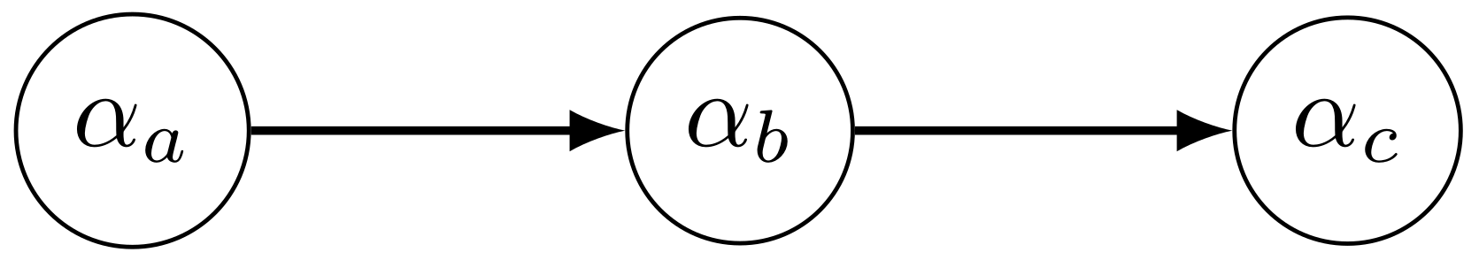
2.2.2. LCDM Structural Model and Attribute Hierarchies

Whereas the LCDM measurement model links the attributes to the manifest variables, the LCDM structural model describes how the attributes relate to each other. Within the traditional LCDM framework, attributes are assumed to be unstructured in the sense that directional or hierarchical relationships among attributes are not assumed nor specified [16]. However, as [15] notes, hierarchical structures naturally arise in psychological and educational contexts (e.g., [32,33,34]).
In general, directional arrangements among attributes imply that certain attribute profiles are unlikely to exist in the population. For instance, in an analysis of a three-attribute English proficiency assessment, [16] found evidence that the attributes formed an attribute hierarchy such that an individual needed to posses attribute α a (i.e., lexical rules) before possibly possessing attribute α b (i.e., cohesive rules), which, in turn, needed to be possessed before possibly possessing attribute α c (i.e., morphosyntatic rules). The existence of a hierarchy was supported as over 95% of individuals were classified into one of four profiles associated with a hierarchy even though there were eight possible classes. To be precise, the authors found evidence of a linear hierarchy (see Figure 1).
From a statistical perspective, an attribute hierarchy implies the non-existence of certain attribute profiles (or latent classes). If an attribute hierarchy truly exists in the population, DCMs that do not account for the hierarchy are likely to misfit the data. If the number of attributes is large, the LCDM will attempt to estimate 2 A attribute profiles, including those that do not exist. This will likely result in incorrect or unstable parameter estimates and attribute profile misclassifications (e.g., [16,35,36,37]). Ref. [16] addressed this concern by modifying the LCDM to statistically model and test hypotheses about the existence of attribute hierarchies. Their model, called the hierarchical diagnostic classification model (HDCM), was obtained by placing constraints on the structural (and measurement) model to reflect the hypothesis that certain attribute profiles are implausible. Thus, the HDCM models a subset of attribute profiles instead of all possible profiles. Under the linear hierarchy depicted in Figure 1, for instance, the HDCM models A + 1 = 3 + 1 = 4 attribute profiles instead of 2 A = 2 3 = 8 profiles.
The HDCM has been found to be a suitable alternative for modeling DCMs when an attribute hierarchy exists; however, a limitation of this model is that attribute profiles that do not follow the structure of the attribute hierarchy are assumed to have zero probability of existing in the population, inducing what we call a strict hierarchy. Recent research by [35,37], among others, has explored alternative methods for modeling attribute structures; however, their methods also impose the requirement of a strict hierarchical structure. The approach presented in this paper differs from these works as we relaxed the assumption of a strict attribute hierarchy by allowing unlikely attribute profiles to have a non-zero probability of existing in the population (i.e., a “malleable” hierarchy) by parameterizing the structural model as a Bayesian network.

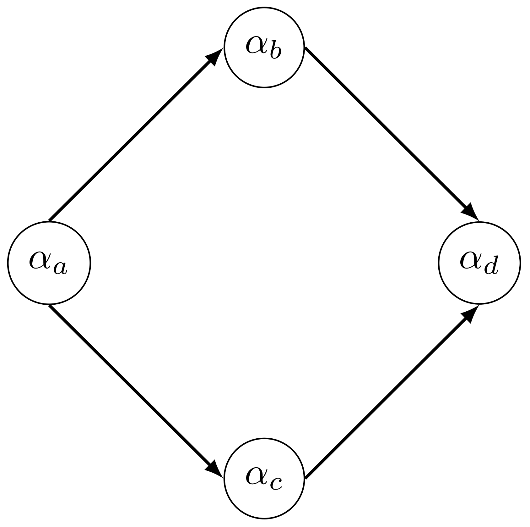
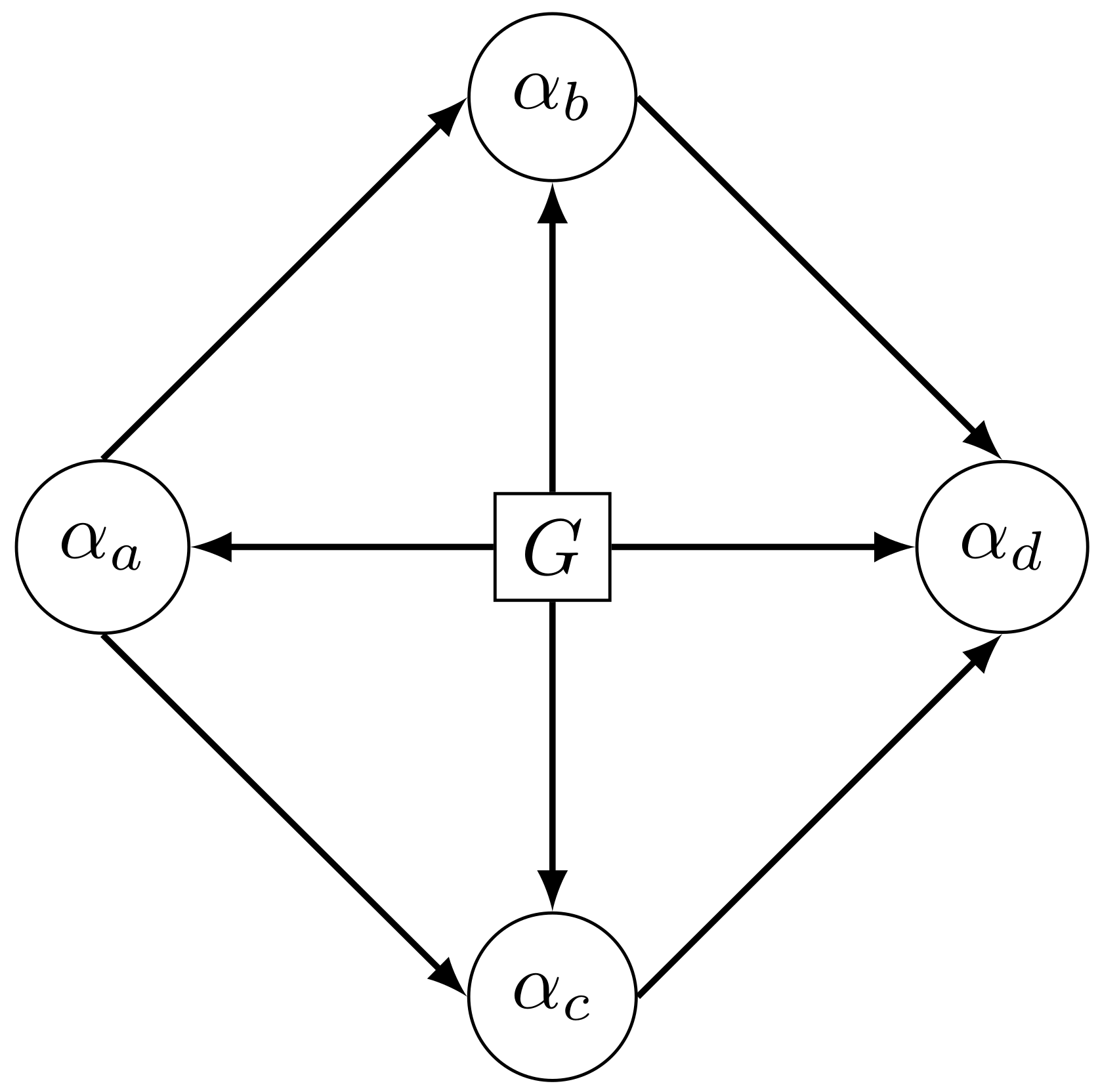
3. Parameterization of the LCDM Structural Model as a Bayesian Network

Ref. [36] showed that the unstructured DCM structural model can be parameterized as a Bayesian network (BN), which they called the saturated BN, and that attribute hierarchies can be derived from and are nested within the saturated BN via a factorization of the joint distribution of the attributes P ( α ) . A major advantage of the BN approach is that it relaxes the overly strict assumption that certain attribute profiles are impossible by permitting unlikely attribute profiles to have a non-zero probability in the population. Relaxing the assumption of a strict attribute hierarchy more closely aligns with empirical findings that it is possible for individuals to possess an attribute that is higher in the hierarchy without first possessing an attribute that is lower in the hierarchy (e.g., an individual possessing attribute α b and α c without necessarily possessing attribute α a in the example of the linear hierarchy in Figure 1).
Several excellent in-depth treatments of BNs can be found in [38,39,40], among others. For our purposes, it suffices to know that a BN consists of two components: (1) a graph—specifically a directed acyclic graph (DAG)—where the elements of the graph consist of nodes (representing random variables) and directed edges (arrows) connecting the nodes and (2) the specification of a joint probability distribution over the DAG. The power of the BN lies in its ability to decompose the joint distribution of the random variables in the DAG as a product of conditional and marginal distributions according to the structure imposed by the directed edges. Importantly, the resulting distributions will have tractable forms that make them easier to work with.

Illustrative Example with a Diamond Attribute Hierarchy

To illustrate, consider the DAG depicted in Figure 2, which represents a diamond attribute hierarchy. This is the attribute structure that we investigated in the case study described later in this paper. Because we have assumed that α is a latent variable, it will possess a distribution, namely the joint distribution P ( α ) = P ( α a , α b , α c , α d ) . We can recover the diamond attribute structure via the following product factorization:
P ( α ) = P ( α a , α b , α c , α d ) = P ( α a ) P ( α b α a ) P ( α c α a ) P ( α d α b , α c ) .
This decomposition follows directly from the product rule of probability [41]. Mathematically, any product decomposition of P ( α a , α b , α c , α d ) is valid; hence, for instance, the product P ( α b ) P ( α a α b ) P ( α c α b ) P ( α d α a , α c ) could have been used instead of the decomposition in Equation (4). However, the former is a more useful representation as it matches the diamond structure in Figure 1 whereas the latter implies a slightly different diamond structure. Using terminology from the BN literature, α a is called a parent of α b and α c (alternatively, the latter are also called children of α a ), α b and α c are parents of α d , and α a is an ancestor of α d (alternatively, α d is a descendant of α a ).
The factorization above shows that the joint distribution P ( α ) is the product of the marginal distribution of α a , the conditional distribution of α b given α a , the conditional distribution of α c given α a , and the conditional distribution of α d given ( α b , α c ) . Because each attribute is assumed to be binary, it follows that
α a Bernoulli ( ρ a ) , α b α a Bernoulli ( ρ b ) , α c α a Bernoulli ( ρ c ) , α d α b , α c Bernoulli ( ρ d ) ,
where ρ z = P ( α z = 1 P ( α z ) ) is the probability that attribute z is a possessed conditional on P ( α z ) . The term P ( α z ) is called the parent set of α z and, conceptually, it represents all the variables in the DAG that have an arrow pointing to α z . For the diamond hierarchy, we see that P ( α a ) is empty since there are no nodes (variables) in the DAG that point to α a , P ( α b ) = { α a } , P ( α c ) = { α a } , and P ( α d ) = { α b , α c } .
We can model the joint distribution P ( α ) via the probabilities ρ a , ρ b , ρ c , and ρ d , which can be accomplished through the latent regression models:
ρ a = exp ( β 0 ) 1 + exp ( β 0 ) , ρ b = exp ( γ 0 + γ 1 α a ) 1 + exp ( γ 0 + γ 1 α a ) , ρ c = exp ( δ 0 + δ 1 α a ) 1 + exp ( δ 0 + δ 1 α a ) , ρ d = exp ( κ 0 + κ 1 α b + κ 2 α c + κ 12 α b α c ) 1 + exp ( κ 0 + κ 1 α b + κ 2 α c + κ 12 α b α c ) ,
where ( β 0 , γ 0 , δ 0 , κ 0 ) are intercept parameters, ( γ 1 , δ 1 , κ 1 , κ 2 ) are main effect (slope) parameters, and κ 12 is a latent interaction effect.
An examination of Equation (6) provides insights into the structure of the attribute hierarchy. First, note that any probability of interest with respect to P ( α ) can be computed directly from the four probabilities in (6). For instance, consider the probability that an individual in the population has attribute profile α = ( 0 , 0 , 0 , 1 ) , which corresponds to possessing attribute α d but not α a , α b , nor α c . Under the BN, this probability is computed as   
P ( α ) = P ( α a = 0 , α b = 0 , α c = 0 , α d = 1 ) = P ( α a = 0 ) P ( α b = 0 α a = 0 ) P ( α c = 0 α a = 0 ) P ( α d = 1 α b = 0 , α c = 0 ) = ( 1 ρ a ) ( 1 ρ b ) ( 1 ρ c ) ρ d = 1 1 + exp ( β 0 ) 1 1 + exp ( γ 0 ) 1 1 + exp ( δ 0 ) exp ( κ 0 ) 1 + exp ( κ 0 ) .
In general, this quantity will be non-zero, which allows for the possibility an individual with attribute profile α to exist in the population even if the diamond hierarchy is correct. By contrast, methods that assume a strict hierarchy will assume that such an individual cannot exist and will therefore fail to accurately identify that individual’s true attribute profile.
A second observation from (6) is that α a directly influences α b and α c through the probabilities ρ b and ρ c , respectively. Hence, α a can be thought of as a direct effect to both α b and α c . Similarly, α b and α c can be thought of as direct effects to α d . Lastly, note that α a affects α d indirectly through the mediating probabilities ρ b and ρ c , showing that the effect of α a on α d is mediated by α b and α c , respectively.
Although the example above corresponds specifically to the diamond attribute hierarchy, the BN approach is general and can be extended to include many more attributes and can also accommodate different types of variables, both observed or latent. This extension is the basis for extending the LCDM structural model for invariance testing in subsequent sections.

4. Measurement Invariance in DCMs

As mentioned in the introduction, measurement invariance (MI) refers to the idea that an assessment should retain all desirable psychometric characteristics when administered across different populations. Within the DCM framework, invariance analyses seek to determine the extent to which the probability of item endorsement for individuals with a given attribute profile α , but whom belong to qualitatively different groups, remains the same. The condition of invariance is said to be satisfied if, conditional on attribute profile α and group membership, the probability of a item endorsement is the same irrespective of group membership [6,42].
Measurement invariance in the context of DCMs is a relatively new area of study; however, several methodological advances have been made in recent years. One line of DCM invariance research investigates invariance with special cases of general DCMs. The majority of research in this area has focused on measurement invariance with the highly restricted DINA model [42,43,44,45,46,47,48,49,50] and many of the listed references have focused on adapting IRT-based measurement invariance (called differential item functioning in the IRT literature) techniques for use in DCMs. The second line of invariance research has examined measurement invariance with general DCMs (e.g., [51,52,53,54]); however, this area appears to be much less studied than the former. Moreover, to the best of our knowledge, with the exception of [50], none of the existing DCM invariance literature has considered attribute-level invariance testing and none has considered invariance testing in the presence of attribute hierarchies.

5. Modifying the LCDM for Invariance Testing

In this section, we modify the LCDM measurement model and BN structural model to allow for invariance testing in the presence of attribute hierarchies. We start by extending the LCDM measurement model, followed by the BN structural model.

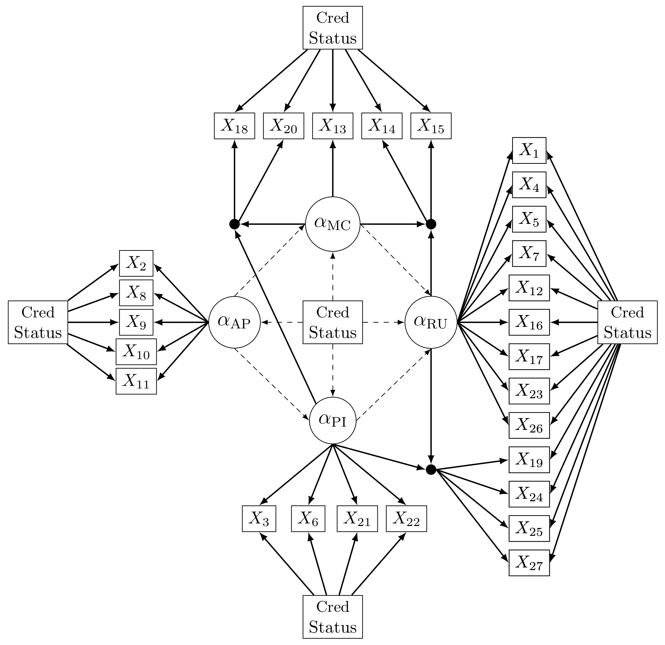
5.1. Specification of the MI-LCDM Measurement Model

The LCDM can be modified to allow for invariance testing in a straightforward way. For convenience, we call the modified LCDM the MI-LCDM. Throughout the remainder of this paper, we consider the case in which there are two groups under investigation; however, we note that the model can be extended to allow for more groups. To start, we introduce the indicator variable G, which takes on a value of 1 if an individual is a member of the focal group and 0 otherwise (i.e., reference group). For concreteness, consider the LCDM for item i as given earlier in (1). In the logit representation, the MI-LCDM for this item is of the form
log P ( X r i = 1 α r , G r ) 1 P ( X r i = 1 α r , G r ) = λ i , 0 + λ i , 1 , ( a ) α r a + λ i , 1 , ( b ) α r b + λ i , 2 , ( a , b ) α r a α r b + G r λ i , 0 + λ i , 1 , ( a ) α r a + λ i , 1 , ( b ) α r b + λ i , 2 , ( a , b ) α r a α r b ,
where parameters with the ★ superscript are called item invariance parameters and represent modifications to their respective counterparts that apply specifically to individuals who are members of the focal group. To illustrate, the parameter λ i , 0 now represents the expected log-odds of item endorsement for members of the reference group who do not possess α a nor α b . The invariance parameter λ i , 0 represents an adjustment to λ i , 0 that applies specifically to members of the focal group who also do not possess α a nor α b . In other words, the intercept for the reference group is λ i , 0 while the intercept for the focal group is λ i , 0 + λ i , 0 .
Similarly, λ i , 0 + λ i , 1 , ( a ) represents the expected log-odds of item endorsement for members of the reference group who possess α a but not α b , and ( λ i , 0 + λ i , 0 ) + ( λ i , 1 , ( a ) + λ i , 1 , ( a ) ) represents the expected log-odds of item endorsement for members of the focal group who possess α a but not α b . The interpretation of the remaining parameters follows a similar logic. In general, the focal group is favored over the reference group (i.e., a higher probability of item endorsement) when the invariance parameter λ i , ( g ) > 0 and the reference group is favored when λ i , ( g ) < 0 , keeping all other parameters constant, where • represents the effect under consideration and ( g ) denotes the focal group index (here, ( g ) = since we only consider two groups). The goal of invariance analyses in this context is to investigate the extent to which λ i , ( g ) results in a meaningful departure from λ i , .
Note that, because attributes are assumed to take on a finite number of states (in our case, two), the scale of the latent attributes is fixed. Importantly, this means that there is no need to identify an anchor item since the scale of the latent variables is completely determined, i.e., a respondent either does/does not possess the attribute under investigation; see [55]. This is in contrast to measurement invariance approaches for factor analysis and item response theory, which require that the latent variables be placed on the same scale for invariance analyses and group comparisons to be meaningful (see [56] for an in-depth discussion of this issue).
With the specification of the MI-LCDM measurement model complete, we now turn our attention to the specification of the modified BN structural model. As previously described, the role of the structural model is to capture and describe the relationships among the attributes. The BN parameterization of the structural model introduced earlier allows for saturated and hierarchical attribute structures to be specified as a series of latent regression models. We now extend these models to allow for invariance testing at the attribute level.

5.2. Specification of the MI-BN Structural Model

For invariance testing at the structural level, the group membership indicator variable G is appended to the structural model as an observed parent node to all attributes, which yields a modified joint distribution. For A attributes, the joint distribution factorizes as
P ( α , G ) = P ( G ) a = 1 A P α a P ( α a ) , G ,
where P ( G ) is the proportion of respondents in the focal group and the product reflects the hierarchical attribute structure of interest.
Returning to the diamond attribute hierarchy example, the factorized joint distribution for the modified hierarchy is
P ( α , G ) = P ( α a , α b , α c , α d , G ) = P ( G ) P ( α a G ) P ( α b α a , G ) P ( α c α a , G ) P ( α d α b , α c , G ) .
Hence, the conditional distributions for the attributes are
α a G Bernoulli ( ρ ˜ a ) , α b α a , G Bernoulli ( ρ ˜ b ) , α c α a , G Bernoulli ( ρ ˜ c ) , α d α b , α c , G Bernoulli ( ρ ˜ d ) ,
where ρ ˜ z is the modified probability that attribute z is possessed and is conditional on both P ( α z ) and G. For this example, the parent sets are P ( α a ) = { G } , P ( α b ) = { α a , G } , P ( α c ) = { α a , G } , and P ( α d ) = { α b , α c , G } . Figure 3 displays the DAG associated with the modified diamond attribute hierarchy. Note that, because G is an observed variable, it is represented in the DAG as a rectangle instead of a circle.
The latent regression models associated with each ρ ˜ z are given by
ρ ˜ a = exp ( β 0 + G β 0 ) 1 + exp ( β 0 + G β 0 ) , ρ ˜ b = exp ( γ 0 + γ 1 α a + G ( γ 0 + γ 1 α a ) ) 1 + exp ( γ 0 + γ 1 α a + G ( γ 0 + γ 1 α a ) ) , ρ ˜ c = exp ( δ 0 + δ 1 α a + G ( δ 0 + δ 1 α a ) ) 1 + exp ( δ 0 + δ 1 α a + G ( δ 0 + δ 1 α a ) ) , ρ ˜ d = exp ( κ 0 + κ 1 α b + κ 2 α c + κ 12 α b α c + G ( κ 0 + κ 1 α b + κ 2 α c + κ 12 α b α c ) ) 1 + exp ( κ 0 + κ 1 α b + κ 2 α c + κ 12 α b α c + G ( κ 0 + κ 1 α b + κ 2 α c + κ 12 α b α c ) ) .
Similar to the MI-LCDM measurement model, parameters in the MI-BN model with a ★ superscript represent attribute invariance parameters. In this formulation, ( β 0 , γ 0 , δ 0 , κ 0 ) are the intercept parameters for each respective α z -submodel. These parameters are interpreted as the log-odds of possessing attribute α z conditional on membership in the reference group and when all other elements in P ( α z ) are zero. Hence, for instance, in the α b -submodel, γ 0 is the log-odds of possessing attribute α b for members of the reference group who do not posses the prerequisite attribute α a . The parameters ( β 0 , γ 0 , δ 0 , κ 0 ) are adjustments made to the respective counterparts for respondents in the focal group. Thus, for the α b -submodel, γ 0 is the expected change to the log-odds of possessing α b for respondents in the focal group who do not posses α a . The other parameters are interpreted accordingly. Similar to invariance testing at the measurement level, the goal of invariance analyses at the structural level is to evaluate the extent to which the attribute invariance parameters result in a meaningful departure from their respective counterparts.

6. Case Study: Diagnosing Teachers’ Multiplicative Reasoning Skills

The diagnosing teachers’ multiplicative reasoning (DTMR) assessment is a diagnostic assessment developed by [20] to assess teachers’ understanding of the components needed to reason about fraction arithmetic. The assessment was primarily designed for teachers who teach grades 5–7, as these grades are formative for teaching students the fundamentals of arithmetic. The goal of the DTMR is to provide teachers with diagnostic feedback with respect to the attributes measured by the assessment, with the hope that the feedback will help teachers to identify components of reasoning about fraction arithmetic that they have or have not fully mastered.
The assessment consists of 27 dichotomously scored items and measures four attributes that emphasize the components needed for making sense of fraction arithmetic. The first attribute, referent units (RUs), measures the ability to identify the whole to which fractions refer. The second attribute, partitioning and iterating (PI), measures the ability to partition a quantity into equal components and create larger fractions by combining unit fractions. The third attribute, appropriateness (AP), measures the ability to identify an appropriate operation or mathematical expression for a given problem situation based on the text of the problem. The fourth attribute, multiplicative comparison (MC), measures the ability to make comparisons with respect to two quantities and identify the relative proportions between the two. Nineteen items measure a single attribute and eight items measure two attributes. The attributes RU, PI, AP, and MC were each measured by 15, 10, 5, and 5 items, respectively. The Q-matrix for this assessment is given in Table 1.
The dataset analyzed here was collected from a representative sample of 990 in-service middle school mathematics teachers. In the original analysis by [20], the response data were fit with the LCDM with an unstructured attribute pattern; however, [36] found that the patterns of the attribute structure were consistent with that of a diamond attribute hierarchy in which AP ( α a ) is a prerequisite of MC ( α b ) and PI ( α c ), both of which are prerequisites of RU ( α d ). Figure 4 shows the complete path diagram of the hypothesized DTMR model.
In addition to the response data obtained from the assessment, additional teacher information was collected. Of interest to this analysis is the variable MCred, an indicator variable that described the teachers’ credential status. Credentialed teachers were full-time instructors with several years of experience while non-credentialed teachers mainly consisted of early childhood and education majors who were working in the school system as part of their undergraduate training (i.e., teachers-in-training). In this analysis, teacher credential status served as the group covariate, with Mcred = 1 for credentialed teachers and Mcred = 0 otherwise. Approximately 67% (n = 653) of teachers were credentialed at the time of their participation in the study.

7. Bayesian Estimation in JAGS

Given the complexity of the MI-LCDM measurement model and the MI-BN structural model, we implemented a fully Bayesian approach to estimate the DTMR model parameters. More specifically, a Markov Chain Monte Carlo (MCMC) algorithm employing Gibbs sampling was used. The algorithm is implemented in the Bayesian inference software program JAGS (version 4.3.0; [18]) via R. JAGS, which is short for Just Another Gibbs Sampler, simulates a Markov chain for each model parameter by repeatedly sampling from its full conditional distribution over a large number of iterations. JAGS has been widely used for the estimation of psychometric models (e.g., [57,58]) and is known for being a reliable tool for estimating complex models within the Bayesian framework.
In this analysis, we specified two chains, each with a warm-up phase of 5000 iterations followed by 30,000 post warm-up iterations. To reduce the autocorrelation from sequential samples, a thinning period of 3 was specified (e.g., every third sample was kept). Chain convergence was assessed by inspecting the Gelman–Rubin potential scale reduction factor (PSRF, denoted R ^ ) for each estimated parameter [59]. We used the criterion R ^ 1.1 as evidence that the chains converged to the proper posterior distribution. We also visually inspected the traceplots of the post warm-up samples for further evidence of convergence and to assess the mixing of the chains. If the chains did not converge after the specified number of iterations, additional samples were drawn until convergence.

7.1. Posterior Inference for Teachers with Missing Credential Status

The main objective of this analysis was to investigate the invariance parameters; however, the Bayesian framework can also be used to make inferences about other quantities that may be of interest to researchers. With respect to the DTMR dataset, there were several teachers for which credential status information was not available ( n = 16 ). Rather than removing these cases from the analysis, we treated credential status for these cases as Bernoulli random variables. In doing so, the Gibbs sampling algorithm will construct a credential status posterior distribution by drawing a value from its full conditional distribution at each iteration of the Markov chain. The mean of the resulting posterior distribution quantifies the probability that a given teacher possesses their credential given their responses on the assessment.

7.2. Priors for the Item and Structural Model Parameters

In this analysis, we specified (relatively) non-informative priors to allow the data to contribute the most information in describing the posterior distribution of the parameters. The following priors were placed on the measurement model parameters of the MI-LCDM: λ i , 0 N ( 1.096 , 0.25 ) , λ i , 1 , a N ( 0 , 0.25 ) 1 ( · > 0 ) , and λ i , 2 , ( a , a ) N ( 0 , 0.25 ) 1 ( · > 0 ) , where N ( μ , τ ) is the normal distribution with mean μ and precision τ (i.e., the inverse of the variance). The prior for the intercept is centered at −1.096 so that the corresponding probability of item endorsement is around 0.25 when the respondent does not possess any of the attributes measured by the item. The prior for each main effect is centered at 0 and we imposed a constraint where the proposed sample must be greater than 0 to satisfy the monotonicity constraints described by [29]. These constraints ensure that the probability of item endorsement does not decrease for teachers who possess the attribute(s) measured by the item. The prior for the two-way interaction effect between attribute a and a was also centered around 0 and non-negativity constraints were placed so that the probability of item endorsement when a and a were possessed was greater than if only one of the two attributes was possessed. Strictly speaking, the two-way interaction effect is allowed to be negative so long as it is greater than or equal to the negative of min ( λ i , 1 , ( a ) , λ i , 1 , ( a ) ) ; however, to facilitate the use of the general coding scheme introduced in Listing 1, we opted to impose non-negativity constraints instead.
A similar strategy was used to specify the prior distributions for the parameters associated with the MI-BN model; in particular, the intercept parameters ( β 0 , γ 0 , δ 0 , κ 0 ) N ( 0 , 0.25 ) ; the main effects ( β 1 , γ 1 , δ 1 , κ 1 , κ 2 ) N ( 0 , 0.25 ) 1 ( · > 0 ) ; and the latent interaction effect κ 12 N ( 0 , 0.25 ) 1 ( · > 0 ) . Constraints were placed on the main effect and interaction terms to ensure that the probability of possessing a child attribute did not decrease if the parent attribute was possessed. The priors for the item and attribute invariance parameters will be discussed after showing the JAGS code.

7.3. JAGS Syntax for the MI-LCDM Measurement Model

Listing 1 provides a segment of the JAGS code, specifically the portion corresponding to the MI-LCDM measurement model (the complete JAGS syntax can be found in the Supplemental Materials). The label lambdaAM[i] refers to the name of the effect, where the index A = 0 refers to the intercept, A { 1 , 2 , 3 , 4 } refers to the main effect associated with the RU, PI, AP, and MC attribute, respectively (following the order of the columns in the Q-matrix), and A values with two digits refer to interaction effects between the attributes associated with the digits. The component [i] refers to the ith item and labels ending with G refer to invariance parameters. Thus, for instance, lambda24[18] refers to the interaction effect between attributes PI and MC on item 18 ( λ 18 , 2 , ( 2 , 4 ) ) and lambda24G[18] refers to the invariance effect of the corresponding interaction that applies specifically to credentialed teachers ( λ 18 , 2 , ( 2 , 4 ) ).
The label w[person, item, att] is an augmented variable that corresponds to the value α r a q i a and returns α r a if q i a = 1 and 1 otherwise. The value of these components are determined based on the structure of the Q-matrix. This labeling scheme allows us to use the same syntax for all items without having to define a measurement model for each item individually. Line 8 defines the intercept component of the model, where G[person] is the value on the credential status variable that is passed to JAGS as observed data (see supplemental materials for more details). Lines 10–19 define the main effects and lines 21–34 define the interaction effects. Lines 36–38 combine the intercept, main effects, and interaction effects to define the logit of item endorsement. Finally, line 40 specifies the conditional distribution of the item response (i.e., Bernoulli).
Listing 1. JAGS syntax for the MI-LCDM measurement model.
Psych 05 00045 i001a
Psych 05 00045 i001b

7.4. JAGS Syntax for the MI-BN Structural Model

Listing 2 provides the JAGS syntax corresponding to the MI-BN model. Line 4 defines the α AP -submodel, lines 6–11 define the α PI -submodel, lines 13–18 define the α MC -submodel, and lines 20–29 define the α RU -submodel. These are equivalent to the logit-transformed versions of ρ ˜ a , ρ ˜ b , ρ ˜ c , and ρ ˜ d in Equation (12), respectively. The labels delta1AP, etc. correspond to the coefficients of each submodel model, where the attribute labels that the effect applies to have been included for increased readability. Lines 31–34 express the models in the probability metric as the models were originally defined on the logit scale. Finally, the distribution of the attribute parameters is specified on line 36.
Listing 2. JAGS syntax for the MI-BN structural model.
Psych 05 00045 i002a
Psych 05 00045 i002b

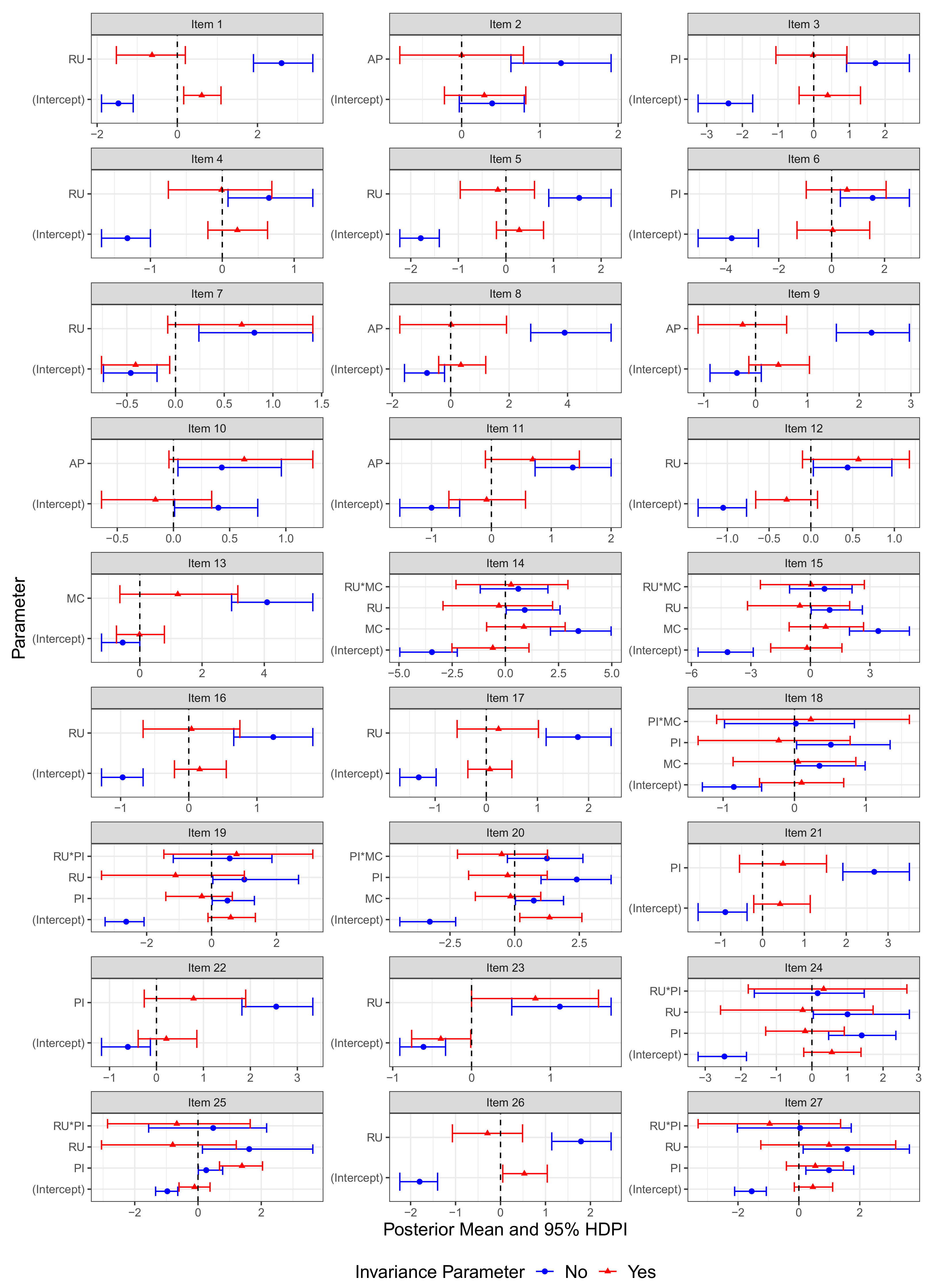
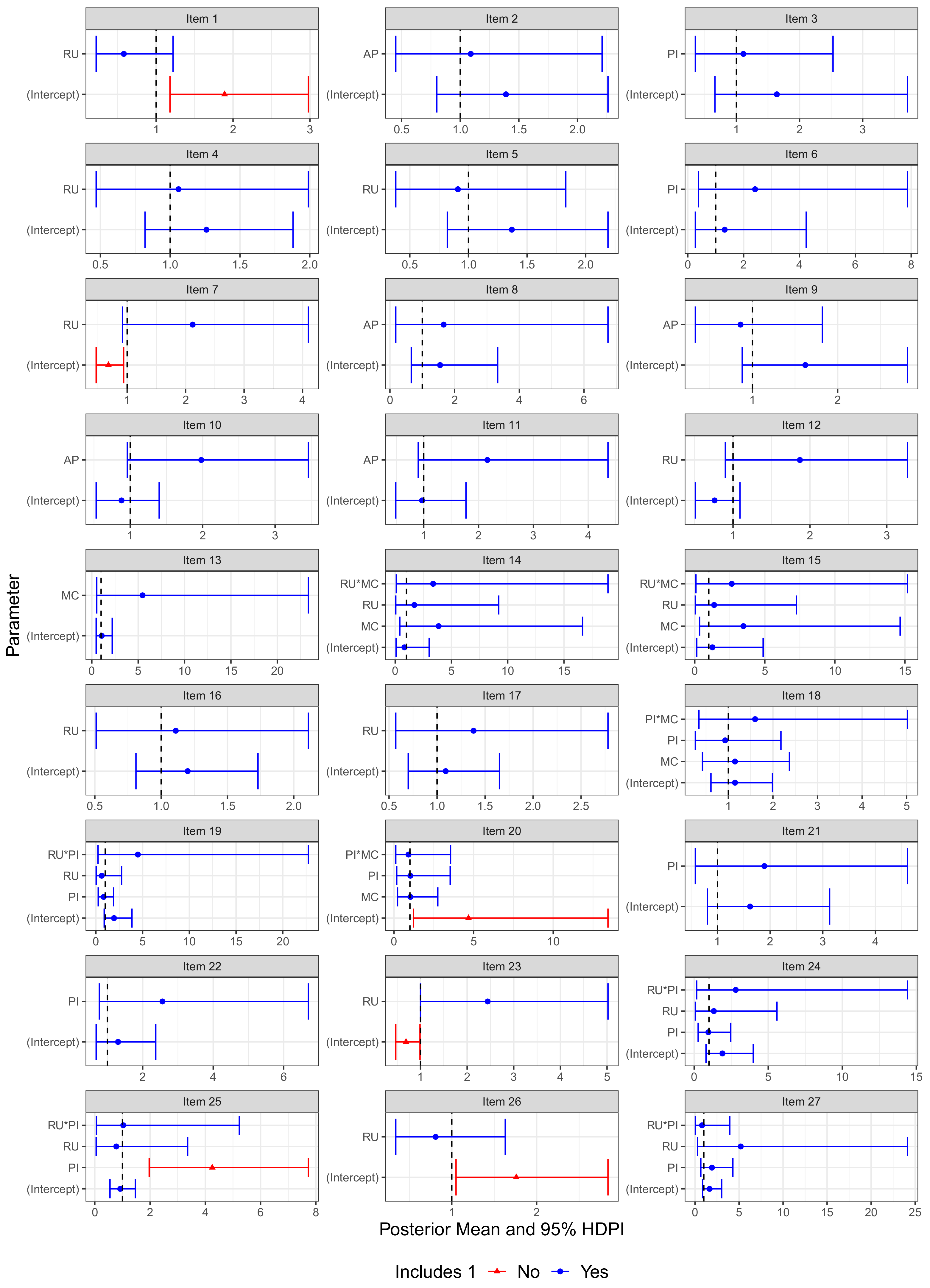
8. Approximate Invariance Testing of the Invariance Parameters

Invariance analyses in the Bayesian framework differ slightly from traditional approaches based on the frequentist framework. A key difference between the two approaches is that the latter tests for ‘strict’ invariance whereas the former tests for approximate invariance (e.g., [60,61]). Briefly, ‘strict’ invariance procedures test whether invariance parameters are exactly zero in the population and inferences are based on asymptotic arguments. By contrast, the approximate invariance approach allows the invariance parameter to live in a neighborhood around zero and the associated effect can still be considered invariant. This assumption is more realistic as parameters across groups are rarely ever exactly equivalent. We refer the reader to [60] for more information on the approximate invariance approach.
In this analysis, the priors for the item invariance parameters were specified as follows: ( λ i , 0 , λ i , 1 , a , λ i , 2 . ( a , a ) ) N ( 0 , 0.25 ) . No constraints were placed on any of the item invariance parameters. The priors for the attribute invariance parameters were specified as follows: ( β 0 , γ 0 , δ 0 , κ 0 ) N ( 0 , 0.25 ) , ( β 1 , γ 1 , δ 1 , κ 1 , κ 2 ) N ( 0 , 0.25 ) , and κ 12 N ( 0 , 0.25 ) . We chose relatively non-informative priors to avoid influencing the parameters too much with the prior distribution.
Following [50], we tested for invariance at the measurement and attribute level by examining the 100 ( 1 ζ ) % highest posterior density interval (HDPI; [62]) of the posterior distribution of the invariance parameters. We conclude that invariance holds with respect to invariance parameter ξ (where ξ generically represents any parameter with a ★ superscript) if the HPDI of ξ contains 0; otherwise, we conclude that the invariance parameter is meaningfully different from 0 and the item or attribute exhibits non-invariance with respect to that parameter. For this analysis, we set ζ = 0.05 so that the HDPI contains 95% of the posterior mass.
For each invariance parameter, we also constructed a measure of effect size by computing the odds ratio. More specifically, exp ( ξ ) can be shown to be the odds ratio of item endorsement for the focal group relative to the reference group. The value exp ( ξ ) implies that the odds of item endorsement for credentialed teachers is exp ( ξ ) times that of non-credentialed teachers. Thus, this value can be interpreted as a measure of effect size, with a value of 1 indicating that the odds between the two groups are equal, a value greater than 1 favoring the credentialed group, and a value less than 1 favoring the reference group. For each iteration of the Markov chain, exp ( ξ ) was computed after ξ was sampled from its respective distribution in the Gibbs sampling algorithm. The resulting distribution approximates the posterior distribution of the odds ratio, which can then be used to construct a HDPI. The effect size of the invariance parameter ξ is said to favor one group over the other if the 95% HDPI of exp ( ξ ) does not contain 1.

9. Results and Interpretation

9.1. Analysis of Markov Chains

Before analyzing the model parameters, the Markov chains were analyzed for evidence of convergence. After eliminating the warm-up samples, R ^ values were less than 1.08 for all parameters, indicating proper chain convergence. In addition, visual inspection of the trace plots showed an adequate mixing of the chains and no abhorrent chain patterns were detected. Thus, no additional samples were obtained beyond the original 30,000 post warm-up samples. Based on these results, we conclude that the chains converged to the posterior distribution and that the results can be meaningfully interpreted. In addition, the effective sample sizes across all parameters ranged from 272.7 to 50,000 (mean = 33,120.6). For item and attribute parameters specifically, these values ranged from 272.7 to 13,180.3 (mean = 2669.8). Overall, these values suggest that the posterior distributions contained adequate resolution, providing evidence that the thinning procedure was effective at mitigating autocorrelation issues associated with Gibbs sampling.

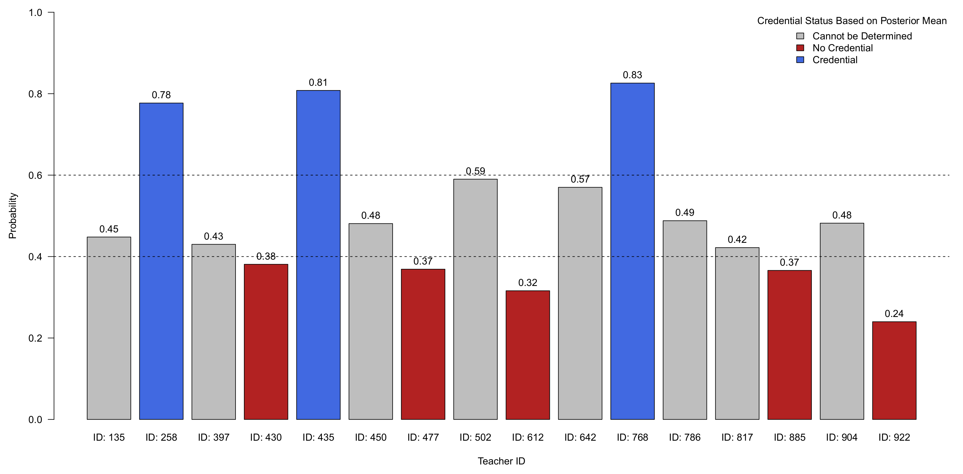
9.2. Analysis of Credential Status

Out of the entire sample, there were n = 16 teachers for whom credential status information was not available. A feature of the Bayesian analysis is the ability to leverage information from the model to estimate the probability that a teacher possesses their credential given their item responses and all other information contained in the model. Three teachers had posterior probabilities greater than 0.60 (range: 0.78–0.83), providing strong evidence that these teachers likely possessed teaching credentials. The posterior probabilities were less than 0.40 for five teachers (range: 0.24–0.38), providing evidence that these teachers likely did not possess teaching credentials (i.e., these teachers are likely to have been student teachers). There was not enough information to confidently classify the remaining eight teachers (range: 0.42–0.59) (see Figure 5).

9.3. Analysis of Measurement Model (Item) Parameters

Figure 6 displays the posterior means and 95% HDPI for all item parameters. Item parameter point estimates ranged from −4.18 to 4.09, with a mean value of 0.21. The point estimates of the odds-ratios ranged from 0.02 to 76.43, with a mean value of 3.89. For all items, the main effects were positive and none of the corresponding 95% HDPIs contained 0, providing evidence that non-credentialed teachers who mastered the attributes measured by the item had a higher probability of providing a correct response than non-credentialed teachers who were non-masters of the measured attributes. The interaction effects were all positive; however, all 95% HDPIs contained 0, suggesting that mastering all attributes measured by the respective items did not incur an additional increase in the probability of correctly answering the item beyond that of mastering the two individual attributes.
Across the 27 items, a total of 6 items (22%) were found to be non-invariant with respect to at least one effect. In particular, items 1, 7, 20, 23, and 26 were found to be non-invariant with respect to the intercept while item 25 was found to be non-invariant with respect to the main effect of attribute PI. The 95% HDPIs of the other invariance parameters contained 0, reflecting the item’s state of partial invariance, i.e., these items exhibit partial invariance but not full invariance. The non-invariant intercept of items 1, 20, and 26 were positive (posterior mean: 0.61, 1.35, 0.53, respectively) indicating that credentialed teachers who were not masters of the measured attributes had a higher probability of correctly answering the item than non-credentialed teachers with similar characteristics. The non-invariant intercept of items 7 and 23 were negative (posterior mean: 0.41 , 0.39 , respectively), indicating that non-credentialed teachers who did not master any of the required attributes had a higher probability of correctly answering the item than credentialed teachers who were also non-masters of the measured attributes. The invariance main effect of attribute PI on item 25 was 1.39, suggesting that credentialed teachers who possessed PI but not RU had a probability of 0.66 of correctly answering the item while non-credentialed teachers with the same characteristics only had a probability of 0.33 of correctly answering the item.
Figure 7 displays the odds ratio distributions for the item invariance parameters. For item 1, the posterior means of the odds-ratio of the non-invariant intercept was 1.98, meaning that the odds that a credentialed teacher who was a non-master of attribute RU provided a correct response was nearly two times larger than that of a non-credentialed teacher with similar mastery status on attribute RU. For item 7, the odds-ratio of the non-invariant intercept was 0.68; for item 20, the odds-ratio of the non-invariant intercept was 4.68; for item 23, the odds-ratio of the non-invariant intercept was 0.69; and, for item 26, the odds-ratio of the non-invariant intercept was 1.76. The odds-ratio of the non-invariant effect of attribute PI for item 25 was 4.25, indicating that the odds that a credentialed teacher who mastered PI provided a correct response was over four times greater than that of non-credentialed teachers.

9.4. Analysis of Structural Model Parameters

Table 2 contains summaries of the posterior distribution for the parameters in the MI-BN structural model. Posterior mean estimates ranged from −3.75 to 2.72, with an average value of 0.22. Posterior mean estimates for the odds ratio—which we computed only for the invariance parameters—ranged from 0.71 to 6.90, with an average value of 1.98. The mean of the intercept for the AP submodel was 0.47, which translates to a model-implied probability of 0.62 of possessing the AP attribute for teachers who were not credentialed. The posterior mean of the invariance intercept parameter was 0.16; however, the 95% HDPI contained 0, providing evidence that the log-odds (and, hence, probability) of mastering the AP attribute does not differ meaningfully from that of non-credentialed teachers. The posterior means and 95% HDPIs of the main effect of AP for the PI and MC submodels were both positive and did not contain 0, suggesting that non-credentialed teachers who possessed AP were much more likely to possess PI and MC compared to non-credentialed teachers who did not possess AP. The 95% HDPI for the invariance main effect of AP for the PI and MC submodels both contained 0, suggesting that credentialed teachers who possessed AP did not have an advantage or disadvantage relative to non-credentialed teachers who also possessed AP. The invariance intercept terms for the PI and MC submodels also contained 0, suggesting that credentialed and non-credentialed teachers who did not possess AP did not differ from each other. A similar trend was observed for the invariance parameters in the RU submodel. In particular, the invariance intercept term, invariance main effect terms of PI and MC, and the invariance interaction effect of PI and MC all contained 0 in their respective HDPIs, suggesting no difference between credentialed and non-credentialed teachers with respect to each of the effects. Because all invariance parameters in the structural model were found to not be meaningfully different from 0, we conclude that there is evidence of full structural (attribute) invariance.

9.5. Model Comparisons

To provide a point of comparison, we compared the relative model fit of the original invariance model (Model 1) to three simpler models via the deviance information criterion (DIC; [63]), where smaller values are generally considered to be indicators of a better model fit. The simpler models impose constraints on the measurement and/or attribute invariance parameters (i.e., parameters with a ★ superscript). The simpler models were: a model that assumes attribute invariance but not measurement invariance (i.e., the group covariate is removed from the structural model but kept in the measurement model; Model 2), a model that assumes measurement invariance but not structural invariance (i.e., the group covariate is removed from the measurement model but kept in the structural model; Model 3), and a model that assumes both measurement and structural invariance (i.e., the group covariate is removed from both the measurement and structural models; Model 4). Model 2 results in a reduction of nine parameters relative to Model 1, Model 3 results in a reduction of half the number of parameters in the measurement model relative to Model 1, and Model 4 results in a reduction of half the number of parameters in both the measurement and structural models relative to Model 1. Model 3 deviates from traditional invariance models as invariance testing usually begins at the measurement level and moves up to the structural level; however, we include Model 3 here for the sake of symmetry and completeness. Note that Model 4 is identical to the one previously estimated by [36] and is the most restrictive model as it assumes complete invariance at the measurement and structural levels. Models 2–4 were estimated using the same specifications as those of the original model.
The DIC values for Models 1–4 were 30,636.66, 30,636.66, 30,767.46, and 30,371.10, respectively. In particular, Models 1 and 2 had identical DIC values, suggesting that omitting the group covariate from the structural model had no impact on the model fit. This finding is consistent with the finding above in which we found evidence of full invariance at the attribute level. Model 3 had the largest DIC value, suggesting a worse model fit when the group covariate is omitted from the measurement model. This result also corroborates with the findings above as some invariance parameters at the measurement level were found to differ meaningfully from 0. Model 4 was found to have the smallest DIC value; however, this could be partially attributed to the fact that Model 4 contains half or just under half as many parameters as Models 1–3. Overall, the results from relative model fit comparisons suggest that the original invariance model exhibits a reasonable model fit relative to the simpler invariance models. As a result, we continue to interpret the results from the original invariance model in subsequent sections.

9.6. Intermediate Summary of Results

The analysis of item parameters revealed that 6 out of the 27 items on the DTMR exhibited partial measurement invariance. Five of the six partially invariant items were non-invariant with respect to the intercept and one item was non-invariant with respect to the effect of the PI attribute. With respect to the latter, non-credentialed teachers who did not possess the measured attributes were statistically less likely to provide a correct response to the item than credentialed teachers with similar characteristics. The effect of the former favored the credentialed teachers, meaning that, among teachers who possessed attribute PI, those with credentials were more likely to provide a correct response than those without credentials. All other items of the assessments were found to exhibit full measurement invariance. There is also evidence of full structural invariance, suggesting that the attribute hierarchy holds equally for teachers with different credential status. These findings were corroborated by the relative model fit comparisons. As a result, the analysis of attribute profiles presented in the next section combine the two groups.

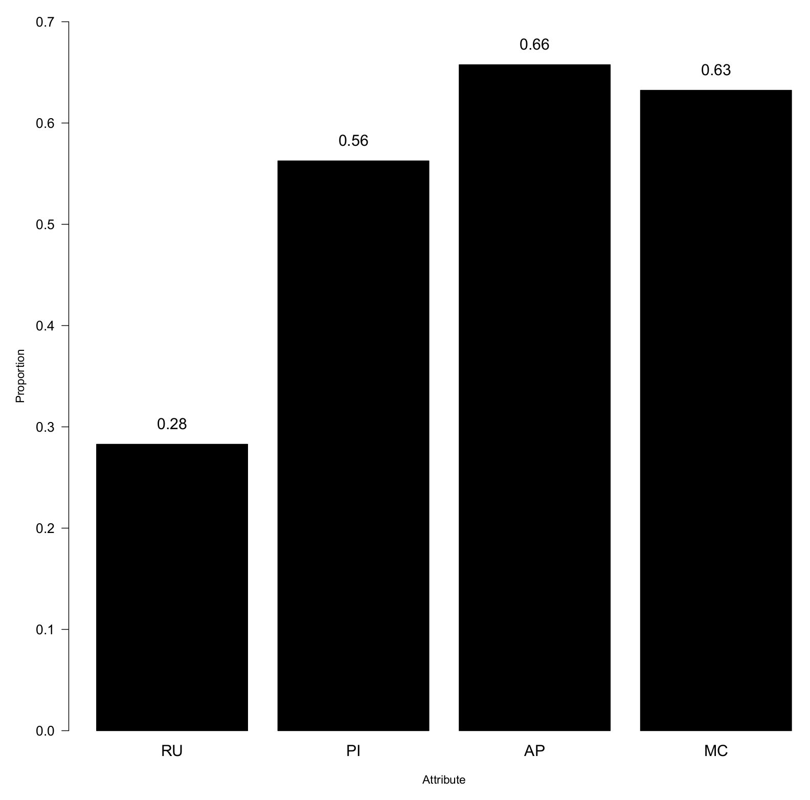
9.7. Analysis of Attribute Profiles

9.7.1. Prevalence of Individual Attributes

Figure 8 contains histograms of the attribute mastery proportions for each attribute across the sample. Attribute RU had the lowest mastery rates, with 28% of teachers possessing this attribute. This was by followed by attributes PI, MC, and AP, with mastery rates of 56%, 63%, and 66%, respectively. This is consistent with previous findings by [20], who observed similar rates under an unstructured attribute configuration. The attribute mastery rates reinforce the plausibility of the hierarchical attribute structure as teachers were more likely to possess attributes higher in the hierarchy compared to those lower in the hierarchy.

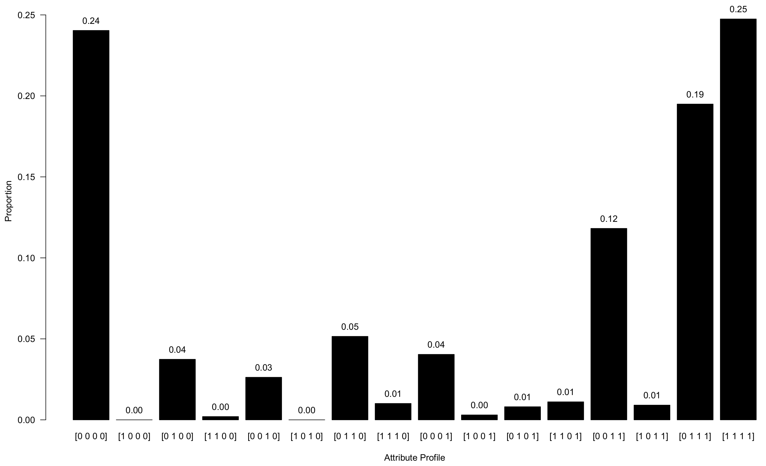
9.7.2. Prevalence of Attribute Profiles

Because the DTMR measures four attributes, there are 16 theoretical attribute profiles, [ α RU , α PI , α AP , α MC ] . However, because of the hypothesized attribute hierarchy, the number of observed attribute profiles was expected to be much smaller. Indeed, the results indicate that this is the case. In particular, zero teachers had profile [ 1 , 0 , 0 , 0 ] or [ 1 , 0 , 1 , 0 ] . This finding makes sense as the attribute hierarchy assumes that it is very unlikely for a teacher to possess RU if they do not possess PI, MC, and AP. It is also unlikely for teachers to possess RU and AP without possessing PI and MC given that, under the hypothesized hierarchy, the latter are descendants of AP and prerequisites for RU.
Figure 9 displays the proportion of teachers who fell into each of the theoretical attribute profiles under each model. As can be seen, the most prevalent attribute profile was [ 1 , 1 , 1 , 1 ] , with 25% of teachers falling into this class, followed by attribute profiles [ 0 , 0 , 0 , 0 ] , [ 0 , 1 , 1 , 1 ] , and [ 0 , 0 , 1 , 1 ] , with 24%, 19%, and 12% of teachers possessing these profiles, respectively. Together, these four attribute profiles made up over 80% of the observed profiles. Moreover, 4% of teachers mastered attribute PI only, 3% mastered attribute AP only, 5% mastered attributes AP and PI, and 4% mastered attribute MC only. Less than 1% of teachers had any of the remaining profiles.

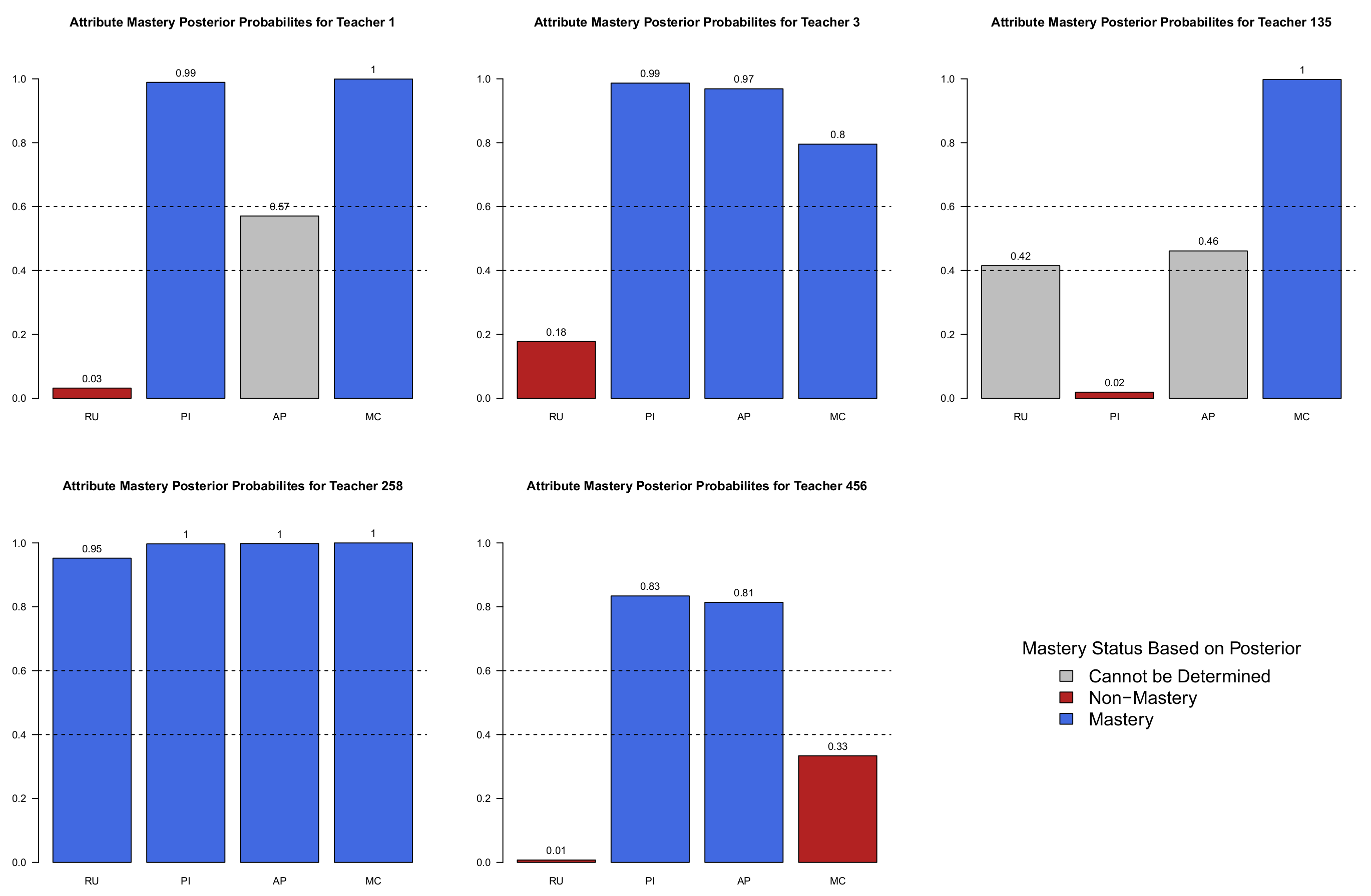
9.7.3. Analysis of Five Randomly Selected Teachers

Figure 10 displays the marginal probabilities of attribute mastery for five randomly selected teachers. The purpose of this analysis was to more closely examine the attribute mastery posterior probabilities and corresponding classifications with a subset of the sample. The figure provides a wealth of information as there was considerable variation in the mastery rates across this subset of teachers. For instance, based on the analysis, we are quite confident that teachers 1, 3, and 456 do not possess attribute RU; however, we are very confident that teacher 258 possesses RU. On the other hand, there was not enough information to unequivocally classify the RU status of teacher 135 based on their response pattern, suggesting that more information with respect to this attribute is needed (e.g., more RU items).

10. Discussion

Invariance testing is an important component of measurement, as researchers aim to develop assessments that are unaffected by factors unrelated to the constructs of interest. If an assessment is found to interact differentially according to group membership, then measures need to be taken to remedy the situation, either by statistically accounting for the non-invariance e.g., partial invariance [64] or by modifying the assessment by removing problematic items. Our goal in this paper was to provide an accessible overview of invariance testing in the DCM framework, specifically when the attributes form attribute hierarchies. To this end, we showed how the LCDM can be extended to allow differential item effects based on group membership to be tested. In addition, we demonstrated how to parameterize the LCDM structural model as a Bayesian network and how this parameterization allows for attribute-level invariance testing. These concepts were illustrated through an in-depth case study with an empirical dataset. The addition of the JAGS code can serve as a starting point for empirical researchers who wish to conduct DCM invariance analyses with their own data.
To the best of our knowledge, the only software programs currently capable of conducting invariance testing in DCMs are the GDINA [65] and CDM [66] packages, both of which are freely available in R. However, the invariance detection methods available in these packages are currently limited to two groups and cannot accommodate various attribute structures or the testing of attribute invariance at the structural level. By contrast, the JAGS code can be easily modified to accommodate more than two groups. For three groups, for instance, this can be accomplished by defining two group covariates G1 and G2, where G1 is an indicator variable that takes on a value of 1 for members of focal group 1 and 0 otherwise, and G2 is a second indicator variable that takes on a value of 1 for members of focal group two and 0 otherwise. An example of the JAGS code for an LCDM measurement model with three groups and four attributes is given in Listing 3. Moreover, because reduced DCMs can be derived from the LCDM through model constraints, the procedures described in this paper apply to reduced DCMs as well.
Listing 3. JAGS syntax for the MI-LCDM measurement model with three groups.
Psych 05 00045 i003a
Psych 05 00045 i003b
We note that although we illustrated the invariance procedure specifically with the diamond attribute structure, the method is very general and the JAGS code can be modified to accommodate the researchers’ specific problem at hand. For instance, the JAGS syntax for a three-attribute linear hierarchy like the one shown in Figure 1, as well as its two-group extension, is provided in Listing 4. Moreover, because attribute hierarchies can be derived from a saturated Bayesian network [36], the procedure and code can also be used for invariance testing with unstructured attributes.
The focus of this paper was to provide an accessible introduction to invariance testing in DCMs in the presence of attribute hierarchies. As a result, we opted to focus on the DTMR as a case study for all analyses. An assumption made in the process was that of a correctly specified diamond attribute hierarchy. Although this assumption was supported by previous empirical research, the extent to which the results from the invariance analyses hold will depend on issues that were not explored in this paper (e.g., parameter recovery, robustness to model misspecifications, etc.). This highlights the need for simulation-based research in this area. Such efforts are currently underway and should provide additional insights above and beyond what this paper can provide (e.g., the impact of incorrectly specifying an attribute hierarchy on invariance analyses).
Listing 4. JAGS syntax for a BN structural model with three-attribute linear hierarchy.
Psych 05 00045 i004a
Psych 05 00045 i004b
In closing, we hope that this paper serves as a useful starting point and guide for applied researchers wishing to conduct invariance analyses with their own data. From our experience, JAGS appears to be well suited for this type of analysis, with the major limitations being mainly computational (e.g., estimation time) as no major issues with respect to the estimation routine itself were found (i.e., we found acceptable evidence of chain convergence). The estimation of the MI-LCDM and MI-BN models took several hours (approximately 7) on an Intel core I5 MacBook Pro with 8GB of RAM. Hence, in addition to the practical contributions of this paper, we also hope that it sparks innovative methodological research into estimation algorithms that can make the estimation of the models more feasible and accessible to applied researchers.

Supplementary Materials

The following supporting information can be downloaded at: https://www.mdpi.com/article/10.3390/psych5030045/s1.

Author Contributions

Conceptualization, A.J.M. and J.T.; methodology, A.J.M. and J.T.; software, A.J.M. and J.T.; validation, A.J.M. and J.T.; formal analysis, A.J.M.; investigation, A.J.M. and J.T.; resources, A.J.M. and J.T.; data curation, A.J.M. and J.T.; writing—original draft preparation, A.J.M.; writing—review and editing, A.J.M. and J.T.; visualization, A.J.M.; supervision, J.T.; project administration, A.J.M. All authors have read and agreed to the published version of the manuscript.

Funding

This research received no external funding.

Institutional Review Board Statement

Not applicable.

Informed Consent Statement

Not applicable.

Data Availability Statement

Code and a simulated version of the dataset can be found in the supplemental materials of this manuscript. Requests for access to the dataset used in the analysis should be directed to Jonathan Templin ([email protected]).

Conflicts of Interest

The authors declare no conflict of interest.

References

  1. Templin, J.; Henson, R.A. Measurement of psychological disorders using cognitive diagnosis models. Psychol. Methods 2006, 11, 287–305. [Google Scholar] [CrossRef] [PubMed]
  2. Wang, D.; Gao, X.; Cai, Y.; Tu, D. Development of a new instrument for depression with cognitive diagnosis models. Front. Psychol. 2019, 10, 1306. [Google Scholar] [CrossRef] [PubMed]
  3. de la Torre, J.; van der Ark, L.A.; Rossi, G. Analysis of clinical data from a cognitive diagnosis modeling framework. Meas. Eval. Couns. Dev. 2018, 51, 281–296. [Google Scholar] [CrossRef]
  4. Ravand, H.; Baghaei, P. Diagnostic classification models: Recent developments, practical issues, and prospects. Int. J. Test. 2020, 20, 24–56. [Google Scholar] [CrossRef]
  5. Leighton, J.; Gierl, M. Cognitive Diagnostic Assessment for Education: Theory and Applications; Cambridge University Press: Cambridge, UK, 2007. [Google Scholar]
  6. Millsap, R.E. Statistical Approaches to Measurement Invariance; Routledge: New York, NY, USA, 2012. [Google Scholar]
  7. Zumbo, B.D. Three generations of DIF analyses: Considering where it has been, where it is now, and where it is going. Lang. Assess. Q. 2007, 4, 223–233. [Google Scholar] [CrossRef]
  8. Hansson, Å.; Gustafsson, J.E. Measurement invariance of socioeconomic status across migrational background. Scand. J. Educ. Res. 2013, 57, 148–166. [Google Scholar] [CrossRef]
  9. American Educational Research Association; American Psychological Association; National Council on Measurement in Education. Standards for Educational and Psychological Testing; American Educational Research Association: Philadelphia, PA, USA, 2014. [Google Scholar]
  10. Kim, E.S.; Yoon, M. Testing measurement invariance: A comparison of multiple-group categorical CFA and IRT. Struct. Equ. Model. 2011, 18, 212–228. [Google Scholar] [CrossRef]
  11. Meredith, W. Measurement invariance, factor analysis and factorial invariance. Psychometrika 1993, 58, 525–543. [Google Scholar] [CrossRef]
  12. Stark, S.; Chernyshenko, O.S.; Drasgow, F. Detecting differential item functioning with confirmatory factor analysis and item response theory: Toward a unified strategy. J. Appl. Psychol. 2006, 91, 1292. [Google Scholar] [CrossRef]
  13. Reise, S.P.; Widaman, K.F.; Pugh, R.H. Confirmatory factor analysis and item response theory: Two approaches for exploring measurement invariance. Psychol. Bull. 1993, 114, 552. [Google Scholar] [CrossRef]
  14. Byrne, B.M.; Shavelson, R.J.; Muthén, B. Testing for the Equivalence of Factor Covariance and Mean Structures: The Issue of Partial Measurement Invariance. Psychol. Bull. 1989, 105, 456–466. [Google Scholar] [CrossRef]
  15. Rupp, A.A.; Templin, J.; Henson, R.A. Diagnostic Measurement: Theory, Methods, and Applications; Guilford Press: New York, NY, USA, 2010. [Google Scholar]
  16. Templin, J.; Bradshaw, L. Hierarchical diagnostic classification models: A family of models for estimating and testing attribute hierarchies. Psychometrika 2014, 79, 317–339. [Google Scholar] [CrossRef] [PubMed]
  17. Almond, R.G.; DiBello, L.V.; Moulder, B.; Zapata-Rivera, J.D. Modeling diagnostic assessments with Bayesian networks. J. Educ. Meas. 2007, 44, 341–359. [Google Scholar] [CrossRef]
  18. Plummer, M. JAGS: A program for analysis of Bayesian graphical models using Gibbs sampling. In Proceedings of the 3rd International Workshop on Distributed Statistical Computing, Vienna, Austria, 20–22 March 2003; Volume 124, pp. 1–10. [Google Scholar]
  19. R Core Team. R: A Language and Environment for Statistical Computing; R Foundation for Statistical Computing: Vienna, Austria, 2022. [Google Scholar]
  20. Bradshaw, L.; Izsak, A.; Templin, J.; Jacobson, E. Diagnosing teachers’ understandings of rational numbers: Building a multidimensional test within the diagnostic classification framework. Educ. Meas. Issues Pract. 2014, 33, 2–14. [Google Scholar] [CrossRef]
  21. Tatsuoka, K.K. Rule space: An approach for dealing with misconceptions based on item response theory. J. Educ. Meas. 1983, 20, 345–354. [Google Scholar] [CrossRef]
  22. Templin, J.; Hoffman, L. Obtaining diagnostic classification model estimates using Mplus. Educ. Meas. Issues Pract. 2013, 32, 37–50. [Google Scholar] [CrossRef]
  23. Chung, M. Estimating the Q-Matrix for Cognitive Diagnosis Models in a Bayesian Framework. Ph.D. Thesis, Columbia University, New York, NY, USA, 2014. [Google Scholar]
  24. Chen, Y.; Liu, Y.; Culpepper, S.A.; Chen, Y. Inferring the number of attributes for the exploratory DINA model. Psychometrika 2021, 86, 30–64. [Google Scholar] [CrossRef]
  25. Culpepper, S.A. Estimating the Cognitive Diagnosis Q Matrix with Expert Knowledge: Application to the Fraction-Subtraction Dataset. Psychometrika 2019, 84, 333–357. [Google Scholar] [CrossRef]
  26. Chung, M. A Gibbs sampling algorithm that estimates the Q-matrix for the DINA model. J. Math. Psychol. 2019, 93, 102275. [Google Scholar] [CrossRef]
  27. Junker, B.W.; Sijtsma, K. Cognitive assessment models with few assumptions, and connections with nonparametric item response theory. Appl. Psychol. Meas. 2001, 25, 258–272. [Google Scholar] [CrossRef]
  28. Hartz, S.M. A Bayesian Framework for the Unified Model for Assessing Cognitive Abilities: Blending Theory with Practicality; University of Illinois at Urbana-Champaign: Urbana-Champaign, IL, USA, 2002. [Google Scholar]
  29. Henson, R.A.; Templin, J.L.; Willse, J.T. Defining a family of cognitive diagnosis models using log-linear models with latent variables. Psychometrika 2009, 74, 191. [Google Scholar] [CrossRef]
  30. de La Torre, J. The generalized DINA model framework. Psychometrika 2011, 76, 179–199. [Google Scholar] [CrossRef]
  31. Sessoms, J.; Henson, R.A. Applications of diagnostic classification models: A literature review and critical commentary. Meas. Interdiscip. Res. Perspect. 2018, 16, 1–17. [Google Scholar] [CrossRef]
  32. Tabatabaee-Yazdi, M. Hierarchical diagnostic classification modeling of reading comprehension. SAGE Open 2020, 10, 2158244020931068. [Google Scholar] [CrossRef]
  33. Ma, W.; Wang, C.; Xiao, J. A Testlet Diagnostic Classification Model with Attribute Hierarchies. Appl. Psychol. Meas. 2023, 47, 183–199. [Google Scholar] [CrossRef] [PubMed]
  34. Zhang, X.; Wang, J. On the sequential hierarchical cognitive diagnostic model. Front. Psychol. 2020, 11, 579018. [Google Scholar] [CrossRef]
  35. Wang, C.; Lu, J. Learning attribute hierarchies from data: Two exploratory approaches. J. Educ. Behav. Stat. 2021, 46, 58–84. [Google Scholar] [CrossRef]
  36. Hu, B.; Templin, J. Using diagnostic classification models to validate attribute hierarchies and evaluate model fit in Bayesian networks. Multivar. Behav. Res. 2020, 55, 300–311. [Google Scholar] [CrossRef]
  37. Ma, C.; Ouyang, J.; Xu, G. Learning latent and hierarchical structures in cognitive diagnosis models. Psychometrika 2023, 88, 175–207. [Google Scholar] [CrossRef]
  38. Pearl, J. Causality: Models, Reasoning, and Inference; Cambridge University Press: Cambridge, UK, 2009. [Google Scholar]
  39. Culbertson, M.J. Bayesian networks in educational assessment: The state of the field. Appl. Psychol. Meas. 2016, 40, 3–21. [Google Scholar] [CrossRef]
  40. Almond, R.G.; Mislevy, R.J.; Steinberg, L.S.; Yan, D.; Williamson, D.M. Bayesian Networks in Educational Assessment; Springer: Berlin/Heidelberg, Germany, 2015. [Google Scholar]
  41. Bishop, C.M. Pattern Recognition and Machine Learning; Springer: Berlin/Heidelberg, Germany, 2006. [Google Scholar]
  42. Liu, Y.; Yin, H.; Xin, T.; Shao, L.; Yuan, L. A comparison of differential item functioning detection methods in cognitive diagnostic models. Front. Psychol. 2019, 10, 1137. [Google Scholar] [CrossRef]
  43. Li, X.; Wang, W.C. Assessment of differential item functioning under cognitive diagnosis models: The DINA model example. J. Educ. Meas. 2015, 52, 28–54. [Google Scholar] [CrossRef]
  44. George, A.C.; Robitzsch, A. Multiple group cognitive diagnosis models, with an emphasis on differential item functioning. Psychol. Test Assess. Model. 2014, 56, 405. [Google Scholar]
  45. de La Torre, J.; Lee, Y.S. A note on the invariance of the DINA model parameters. J. Educ. Meas. 2010, 47, 115–127. [Google Scholar] [CrossRef]
  46. Paulsen, J.; Svetina, D.; Feng, Y.; Valdivia, M. Examining the impact of differential item functioning on classification accuracy in cognitive diagnostic models. Appl. Psychol. Meas. 2020, 44, 267–281. [Google Scholar] [CrossRef] [PubMed]
  47. Hou, L.; de la Torre, J.; Nandakumar, R. Differential item functioning assessment in cognitive diagnostic modeling: Application of the Wald test to investigate DIF in the DINA model. J. Educ. Meas. 2014, 51, 98–125. [Google Scholar] [CrossRef]
  48. Svetina, D.; Feng, Y.; Paulsen, J.; Valdivia, M.; Valdivia, A.; Dai, S. Examining DIF in the context of CDMs when the Q-matrix is misspecified. Front. Psychol. 2018, 9, 696. [Google Scholar] [CrossRef]
  49. Zhang, W. Detecting Differential Item Functioning Using the DINA Model. Ph.D. Thesis, The University of North Carolina at Greensboro, Greensboro, NC, USA, 2006. [Google Scholar]
  50. Li, F. A Modified Higher-Order DINA Model for Detecting Differential Item Functioning and Differential Attribute Functioning. Ph.D. Thesis, University of Georgia, Athens, GA, USA, 2008. [Google Scholar]
  51. Ma, W.; Terzi, R.; de la Torre, J. Detecting differential item functioning using multiple-group cognitive diagnosis models. Appl. Psychol. Meas. 2021, 45, 37–53. [Google Scholar] [CrossRef] [PubMed]
  52. Bozard, J.L. Invariance Testing in Diagnostic Classification Models. Ph.D. Thesis, University of Georgia, Athens, GA, Georgia, 2010. [Google Scholar]
  53. Sun, X.; Wang, S.; Guo, L.; Xin, T.; Song, N. Using a Generalized Logistic Regression Method to Detect Differential Item Functioning with Multiple Groups in Cognitive Diagnostic Tests. Appl. Psychol. Meas. 2023, 47, 328–346. [Google Scholar] [CrossRef] [PubMed]
  54. Bramlett, S.A. A Method for Detecting Measurement Invariance in the Log-linear Cognitive Diagnosis Model. Ph.D. Thesis, University of Georgia, Athens, GA, USA, 2018. [Google Scholar]
  55. Yu, X.; Zhan, P.; Chen, Q. Don’t worry about the anchor-item setting in longitudinal learning diagnostic assessments. Front. Psychol. 2023, 14, 1112463. [Google Scholar] [CrossRef]
  56. Bartholomew, D.J.; Knott, M.; Moustaki, I. Latent Variable Models and Factor Analysis: A Unified Approach; John Wiley & Sons: Hoboken, NJ, USA, 2011. [Google Scholar]
  57. Zhan, P.; Jiao, H.; Man, K.; Wang, L. Using JAGS for Bayesian cognitive diagnosis modeling: A tutorial. J. Educ. Behav. Stat. 2019, 44, 473–503. [Google Scholar] [CrossRef]
  58. Levy, R.; Mislevy, R.J. Bayesian Psychometric Modeling; CRC Press: Boca Raton, FL, USA, 2017. [Google Scholar]
  59. Gelman, A.; Rubin, D.B. Inference from iterative simulation using multiple sequences. Stat. Sci. 1992, 7, 457–472. [Google Scholar] [CrossRef]
  60. Depaoli, S. Bayesian Structural Equation Modeling; Guilford Publications: New York, NY, USA, 2021. [Google Scholar]
  61. Muthén, B.; Asparouhov, T. BSEM measurement invariance analysis. Mplus Web Notes 2013, 17, 1–48. [Google Scholar]
  62. Gelman, A.; Carlin, J.B.; Stern, H.S.; Dunson, D.B.; Vehtari, A.; Rubin, D.B. Bayesian Data Analysis; CRC Press: Boca Raton, FL, USA, 2013. [Google Scholar]
  63. Spiegelhalter, D.J.; Best, N.G.; Carlin, B.P.; Van Der Linde, A. Bayesian measures of model complexity and fit. J. R. Stat. Soc. Ser. B Stat. Methodol. 2002, 64, 583–639. [Google Scholar] [CrossRef]
  64. Millsap, R.E. Testing measurement invariance using item response theory in longitudinal data: An introduction. Child Dev. Perspect. 2010, 4, 5–9. [Google Scholar] [CrossRef]
  65. Ma, W.; de la Torre, J. GDINA: An R package for cognitive diagnosis modeling. J. Stat. Softw. 2020, 93, 1–26. [Google Scholar] [CrossRef]
  66. Robitzsch, A.; Kiefer, T.; George, A.C.; Uenlue, A.; Robitzsch, M.A. Package ‘CDM’. In Handbook of Diagnostic Classification Models; Springer: New York, NY, USA, 2022. [Google Scholar]
Figure 1. Example of a linear attribute hierarchy.
Psych 05 00045 g001
Figure 2. Example of a diamond attribute hierarchy.
Psych 05 00045 g002
Figure 3. Modified linear attribute hierarchy with indicator variable G.
Psych 05 00045 g003
Figure 4. DTMR path diagram. Note: The dashed lines represent the structural model and the solid lines represent the measurement model. The solid circles indicate a complex loading structure among the attributes that point to them. For instance, the measurement model for variable X 18 includes the main effects of α MC and α PI , as well as their latent interaction.
Psych 05 00045 g004
Figure 5. Posterior inference of teachers with missing credential status variable.
Psych 05 00045 g005
Figure 6. Posterior means and 95% HDPI for item parameters. Note: to avoid overlap, the points and lines have been slightly dodged.
Psych 05 00045 g006
Figure 7. Posterior odd ratio means and 95% HDPI for item invariance parameters.
Psych 05 00045 g007
Figure 8. Prevalence of individual attributes.
Psych 05 00045 g008
Figure 9. Prevalence of attribute profiles.
Psych 05 00045 g009
Figure 10. Attribute analysis for five randomly selected teachers.
Psych 05 00045 g010
Table 1. DTMR Q-matrix.
ItemReferent Units, α RU Partitioning and Iterating, α PI Appropriateness, α AP Multiplicative Comparisons, α MC
11000
20010
30100
41000
51000
60100
71000
80010
90010
100010
110010
121000
130001
141001
151001
161000
171000
180101
191100
200101
210100
220100
231000
241100
251100
261000
271100
Table 2. Bayesian network structural model posterior summaries.
Odds Ratio
SubmodelEffectNotationMean (SD)95% HDPIMean (SD)95% HDPI
APIntercept β 0 0.47 (0.23)(0.04, 0.93)
β 0 0.16 (0.27)(−0.38, 0.69)1.22 (0.34)(0.68, 2.00)
PIIntercept γ 0 −1.37 (0.50)(−2.47, −0.53)
γ 0 −0.07 (0.59)(−1.16, 1.14)1.12 (0.89)(0.31, 3.11)
AP Main Effect γ 1 2.54 (0.54)(1.59, 3.69)
γ 1 0.21 (0.63)(−1.06, 1.43)1.51 (1.04)(0.35, 4.18)
MCIntercept δ 0 −1.31 (0.47)(−2.31, −0.46)
δ 0 0.43 (0.54)(−0.57, 1.52)1.79 (1.18)(0.57, 4.59)
AP Main Effect δ 1 2.72 (0.53)(1.77, 3.80)
δ 1 −0.11 (0.61)(−1.33, 1.04)1.08 (0.69)(0.26, 2.83)
RUIntercept κ 0 −3.75 (0.75)(−5.35, −2.46)
κ 0 −0.87 (1.06)(−3.03, 1.14)0.71 (0.91)(0.05, 3.13)
PI Main Effect κ 1 2.08 (0.87)(0.41, 3.85)
κ 1 −0.13 (1.20)(−2.59, 2.14)1.76 (3.22)(0.07, 8.47)
MC Main Effect κ 2 0.97 (0.62)(0.06, 2.33)
κ 2 1.31 (1.10)(−0.85, 3.52)6.90 (11.66)(0.43, 33.88)
PI × MC Interaction κ 12 1.07 (0.83)(−0.54, 2.73)
κ 12 −0.33 (1.26)(−2.74, 2.24)1.80 (6.79)(0.06, 9.42)
Note: Terms with a ★ superscript are attribute invariance parameters and represent modifications to the their non-★ counterparts.
Disclaimer/Publisher’s Note: The statements, opinions and data contained in all publications are solely those of the individual author(s) and contributor(s) and not of MDPI and/or the editor(s). MDPI and/or the editor(s) disclaim responsibility for any injury to people or property resulting from any ideas, methods, instructions or products referred to in the content.

