
A Tutorial on How to Conduct Meta-Analysis with IBM SPSS Statistics


Abstract
1. Introduction
1.1. Steps of Meta-Analysis
- The research question should be formulated.
- A decision should be made on how to select appropriate studies from the collected studies.
- Appropriate studies should be collected according to research questions and keywords.
- Quality control/sensitivity analyses should be done.
- The effect size to be used in the selected studies should be decided and calculated for each study.
- The data should be pooled and a summary measure and confidence interval should be calculated.
- Additional analyses (heterogeneity, publication bias, etc.) should be done.
- Moderator analyses for moderator variables should be performed.
- Results should be interpreted and inferences should be made.
- In addition, the details of the above-mentioned steps should be reported together with the meta-analysis findings.
1.2. Software Options
1.3. Properties of IBM SPSS Statistics
1.3.1. Main Analyses
1.3.2. Publication Bias Analyses
1.3.3. Subgroup Analyses and Meta-Regression
1.4. Steps of Conducting Meta-Analysis in IBM SPSS Statistics
- Step 1: Prepare your data set
- Step 2: Open IBM SPSS Statistics and import your data set
- Select File > Import Data > Excel.
- Step 3: Open Meta Analysis menu
- Select Analyze > Meta Analysis.
- Step 4: Calculate mean effect size
- Select Analyze > Meta Analysis > Continuous Outcomes > Raw Data…
- Add the variables of the treatment group (sample size, mean, and SD) into the ‘Treatment Group’ box
- Add the variables of the control group (sample size, mean, and SD) into the ‘Control Group’ box
- Add the identifying variable (Authors’ names) into the ‘Study ID’ box
- Select the effect size type (Cohen’s d, Hedges’ g, Glass’ delta, Unstandardized Mean Difference) in the ‘Effect Size’ box
- Select the model type (fixed-effect or random-effects) under the ‘Model’ box
- Click ‘OK’
- Select Analyze > Meta Analysis > Binary Outcomes > Pre-Calculated Effect Size
- Select the effect size type (Logg Odds Ratio, Peto’s Logg Odds Ratio, Logg Risk Ratio, and Risk Difference) in the ‘Effect Size’ box
- Add the effect size variable (e.g., Logg Odds Ratio) into the ‘Effect Size’ box
- Add the variance variable into the ‘Variance’ box
- Alternatively, add the standard error variable into the ‘Standard Error’ box
- Add the identifying variable (Authors’ names) into the ‘Study ID’ box
- Select the model type (fixed-effect or random-effects) under the ‘Model’ box
- Click ‘OK’
- Step 5: Check heterogeneity
- Select Analyze > Meta Analysis > Continuous Outcomes > Raw Data…
- Click on the ‘Print’ dialog
- Check the dialog boxes labeled as ‘Test of homogeneity’ and ‘Heterogeneity measures’
- Click ‘Continue’ to go back to the main screen
- Click ‘OK’
- Step 6: Create plots
- Select one of the input screens under the Meta Analysis menu
- For example, Select Analyze > Meta Analysis > Continuous Outcomes > Raw Data
- Click on the ‘Plot’ dialog
- Select ‘Forest Plot’
- Check the dialog box under the ‘Display Columns’
- Decide ‘Position of plot column’, ‘Annotations’, and ‘Reference lines’
- Click ‘Continue’ to go back to the main screen
- Click ‘OK’
- Step 7: Assess publication bias
- Select one of the input screens under the Meta Analysis menu
- For example, Select Analyze > Meta Analysis > Continuous Outcomes > Raw Data
- Click on the ‘Bias’ dialog
- Select ‘Egger’s regression-based test’
- Check the dialog boxes under the ‘Include intercept in regression’ and ‘Estimates statistics based on t-distribution’
- Click ‘Continue’ to go back to the main screen
- Click ‘OK’
- Select one of the input screens under the Meta Analysis menu
- For example, Select Analyze > Meta Analysis > Continuous Outcomes > Raw Data
- Click on the ‘Trim-and-Fill’ dialog
- Select ‘Estimate number of missing studies’
- Check the dialog boxes under the ‘Side to Impute Studies’ as left or right. Another option is to click on ‘Determined by the slopes of Egger’s test’
- Other options can be determined by clicking the boxes under ‘Method’, ‘Iteration Process’
- Click ‘Continue’ to go back to the main screen
- Click ‘OK’
- Step 8: Perform subgroup analyses
- Select one of the input screens under the Meta Analysis menu
- For example, Select Analyze > Meta Analysis > Continuous Outcomes > Raw Data
- Click on the ‘Analysis’ dialog
- Add the variables of interest (categorical moderator) from the ‘Variables’ box into the ‘Subgroup Analysis’ box
- Click ‘Continue’ to go back to the main screen
- Click ‘OK’
- Step 9: Perform meta-regression analyses
- Select Analyze > Meta Analysis > Meta Regression
- Add the effect size variable (e.g., Cohen’s d) from the ‘Variables’ box into the ‘Effect size’ box
- Add the effect size variance from the ‘Variables’ box into the ‘Variance’ box. Alternatively, one can use the standard error or weight of the effect size
- Add the variables of interest (continuous moderator) from the ‘Variables’ box into the ‘Covariate(s)’ box
- Add the variables of interest (categorical moderator) from the ‘Variables’ box into the ‘Factor(s)’ box
- Click ‘Continue’ to go back to the main screen
- Click ‘OK’
2. Empirical Examples
2.1. Example 1 (Standardized Mean Difference)
- Select Analyze > Meta Analysis > Continuous Outcomes > Pre-Calculated Effect Size
- Select File > Open > Data
- Select “Files of Type” as “Excel”
- Find the data > Open
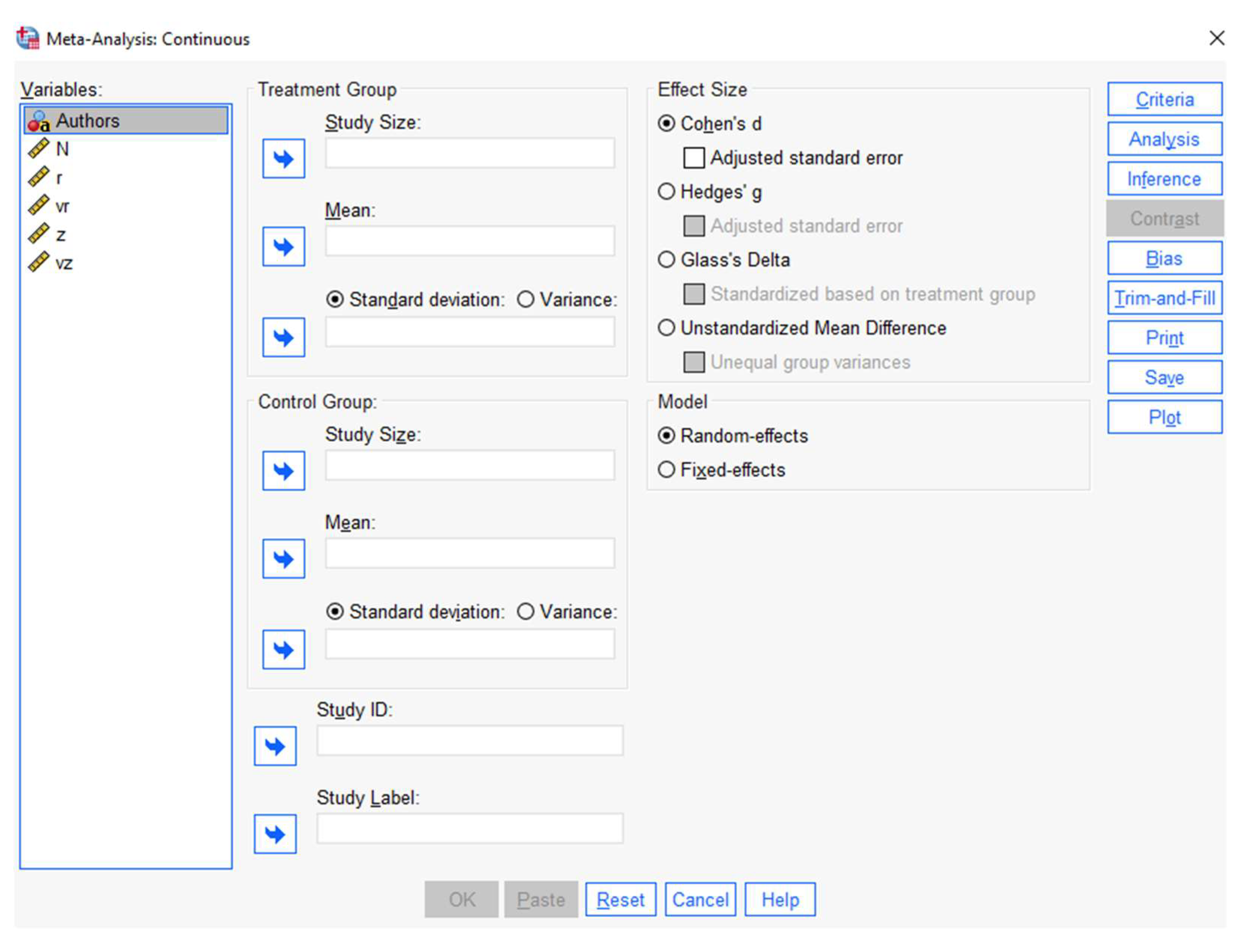
- Select Analyze > Meta Analysis > Continuous Outcomes > Raw Data (see Figure 4)

- Add the variables of the treatment group (sample size, mean, and SD) into the ‘Treatment Group’ box
- Add the variables of the control group (sample size, mean, and SD) into the ‘Control Group’ box
- Add the identifying variable (Authors’ names [Study]) into the ‘Study ID’ box
- Select the effect size type as ‘Hedges’ g’ in the ‘Effect Size’ box
- Select the model type ‘Random-effects’ under the ‘Model’ box
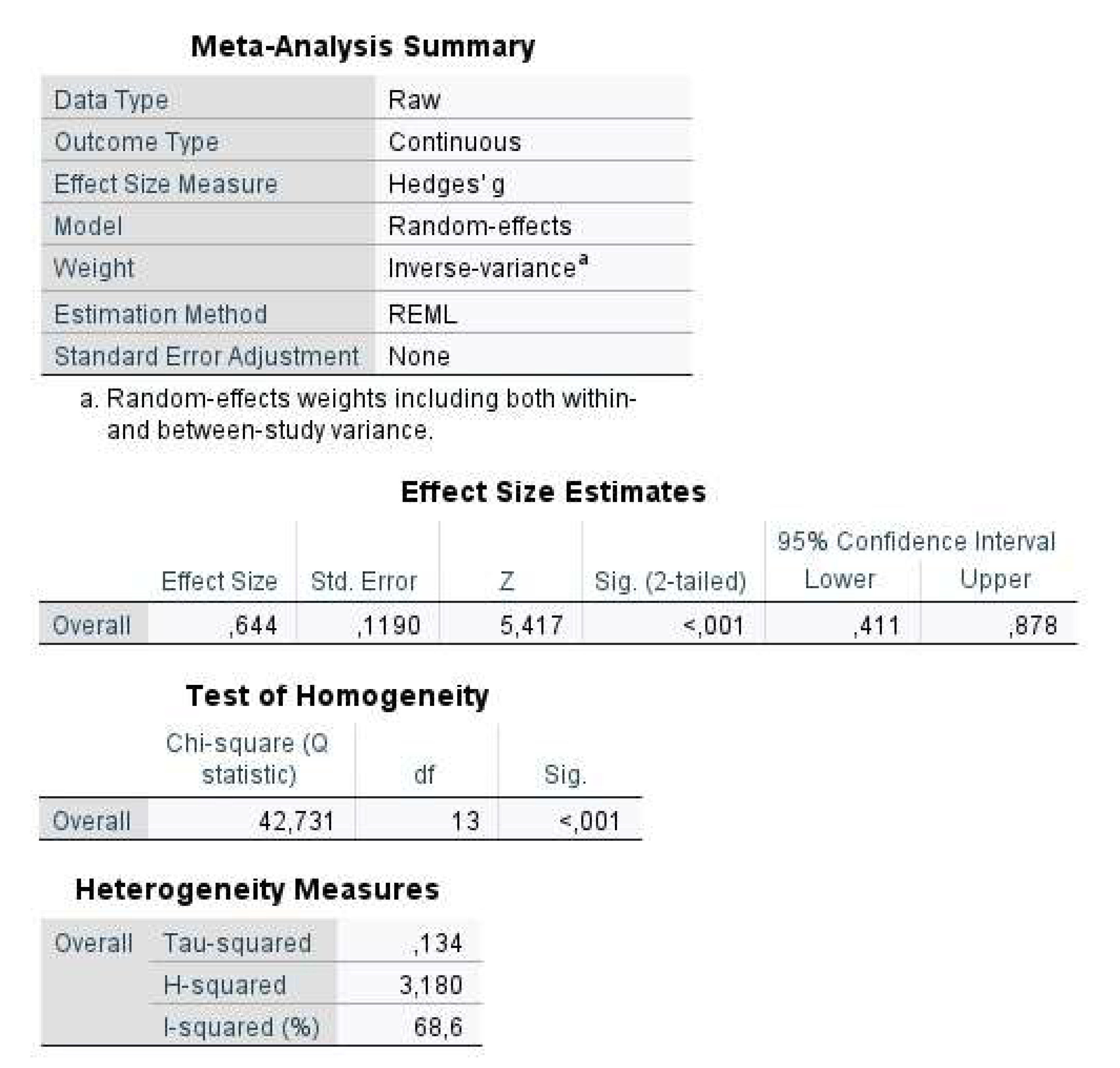
- Open ‘Print’ Dialogue > Select the ‘Test of homogeneity’ and ‘Heterogeneity Measures’ > Click ‘Continue’ (see Figure 5)
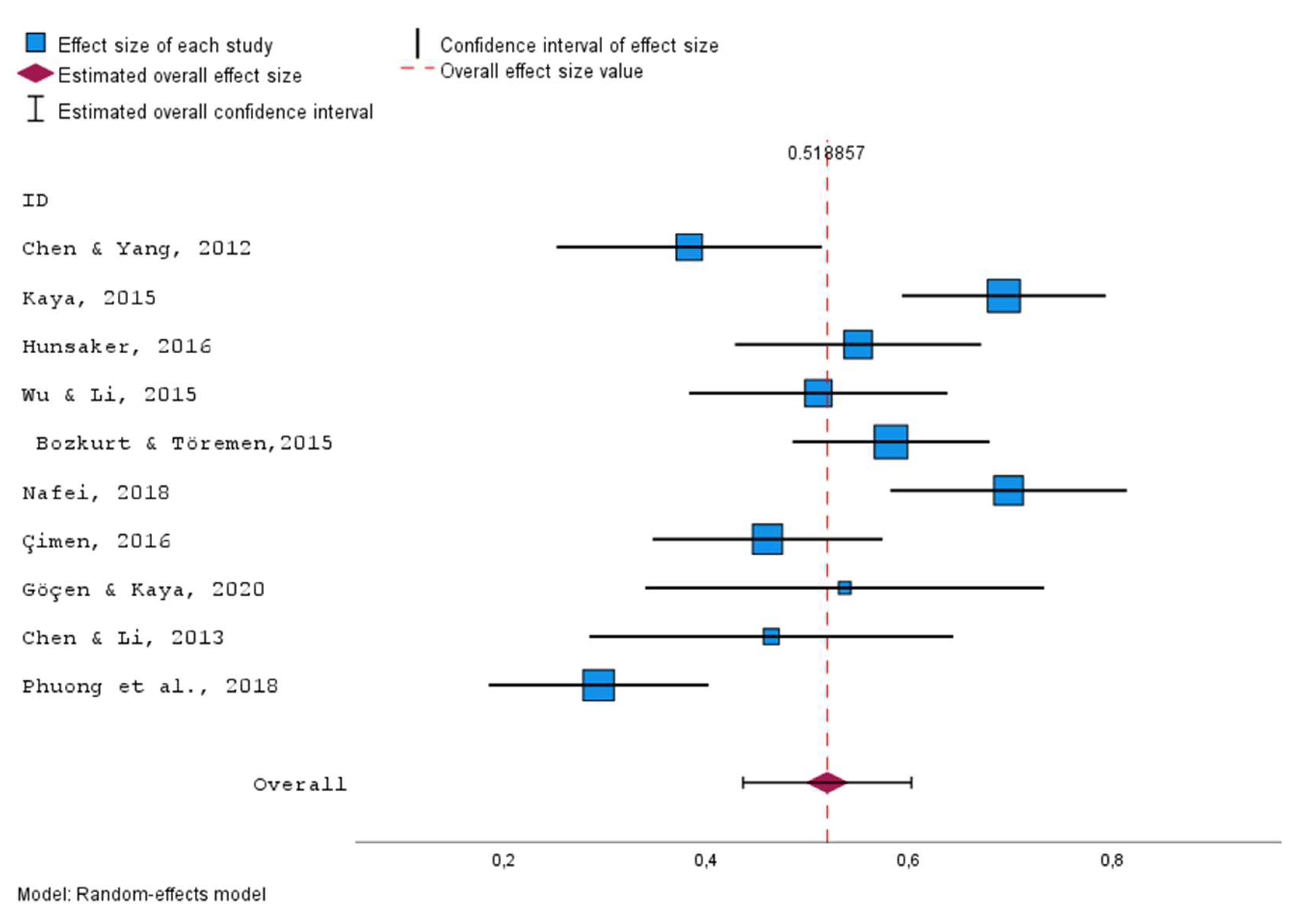
- Open ‘Plot’ Dialogue > Select ‘Forest Plot’ box and all the ‘Display Columns’ boxes > Click ‘Continue’
- Click ‘OK’ (see Figure 6)
2.2. Example 2 (Odds Ratio)
- Select Analyze > Meta Analysis > Binary Outcomes > Pre-Calculated Effect Size
- An easier way to do this is to conduct the analysis using raw data when you have the data ready as entered in Excel. For this option, the following steps can be used.
- Select File > Open > Data
- Find the data > Open
- Select Analyze > Meta Analysis > Binary Outcomes > Raw Data
- Add the variables of the experimental group (success and failure) into the ‘Treatment Group’ box
- Add the variables of the control group (success and failure) into the ‘Control Group’ box
- Add the identifying variable (Authors’ names [Study]) into the ‘Study ID’ box
- Select the effect size type as ‘Log Odds Ratio’ in the ‘Effect Size’ box
- Select the model type ‘Random-effects’ under the ‘Model’ box
- Open ‘Print’ Dialogue > Select the ‘Test of homogeneity’ and ‘Heterogeneity Measures’ > Click ‘Continue’ (see Figure 9)
- Open ‘Plot’ Dialogue > Select ‘Forest Plot’ box and all ‘Display Columns’ boxes > Select ‘Overall effect size’ box > Click ‘Continue’
- Click ‘OK’ (see Figure 10)
2.3. Example 3 (Correlation)
- Select Analyze > Meta Analysis > Continuous Outcomes > Pre-Calculated Effect Size
- Add the effect size variable (e.g., z) into the ‘Effect Size’ box
- Add the variance variable (e.g., vz) into the ‘Variance’ box
- Add the identifying variable (e.g., authors) into the ‘Study ID’ box
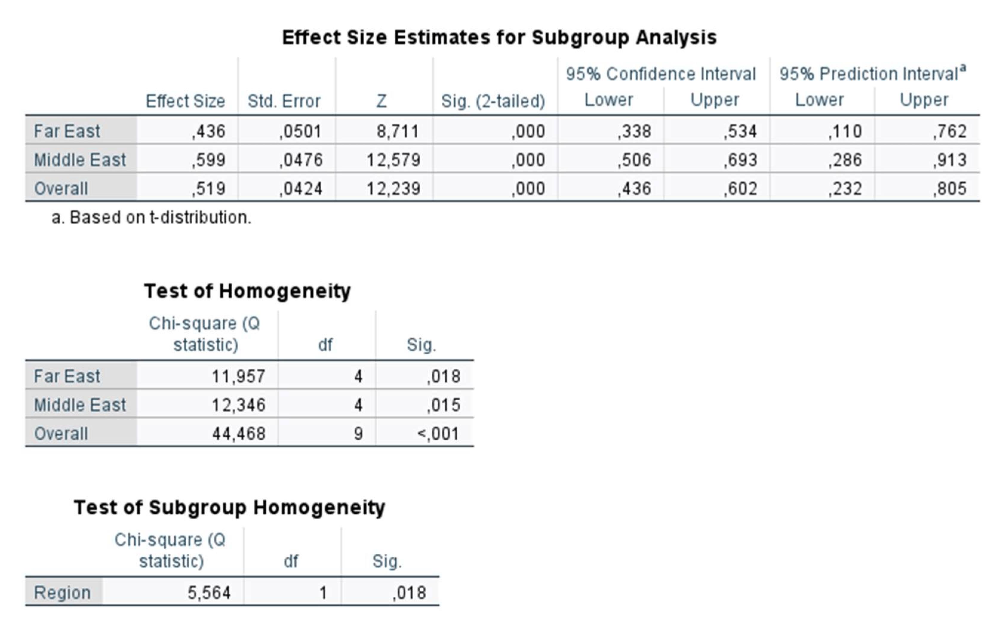
- Select the model type as random-effects under the ‘Model’ box
- Click ‘OK’ (see Figure 14)
- Select Analyze > Meta Analysis > Meta Regression
- Add the effect size variable (e.g., z) into the ‘Effect Size’ box
- Add the variance variable (e.g., vz) into the ‘Variance’ box
- Add the continuous variable (e.g., FemalePercent) into the ‘Covariate(s)’ box
- Add the categorical variable (e.g., Region) into the ‘Factor(s)’ box
- Select the model type as random-effects under the ‘Model’ box
- Click ‘OK’ (see Figure 19)
3. Conclusions
Supplementary Materials
Author Contributions
Funding
Institutional Review Board Statement
Informed Consent Statement
Data Availability Statement
Conflicts of Interest
References
- Eysenck, H.J. The Effects of Psychotherapy: An Evaluation. J. Consult. Psychol. 1952, 16, 319–324. [Google Scholar] [CrossRef] [PubMed]
- Smith, M.L.; Glass, G.V. Meta-Analysis of Psychotherapy Outcome Studies. Am. Psychol. 1977, 32, 752–760. [Google Scholar] [CrossRef] [PubMed]
- Eysenck, H.J. An Exercise in Mega-Silliness. Am. Psychol. 1978, 33, 517. [Google Scholar] [CrossRef]
- Lipsey, M.W.; Wilson, D.B. Practical Meta-Analysis; Applied social research methods series; Sage Publications: Thousand Oaks, CA, USA, 2001; ISBN 978-0-7619-2167-7. [Google Scholar]
- Pearson, K. Report on Certain Enteric Fever Inoculation Statistics. BMJ 1904, 3, 1243–1246. [Google Scholar]
- Rosenthal, R. Combining Results of Independent Studies. Psychol. Bull. 1978, 85, 185–193. [Google Scholar] [CrossRef]
- Glass, G.V.; McGaw, B.; Smith, M.L. Meta-Analysis in Social Research; Sage Publications: Beverly Hills, CA, USA, 1981; ISBN 978-0-8039-1633-3. [Google Scholar]
- Hedges, L.V. Fitting Categorical Models to Effect Sizes from a Series of Experiments. J. Educ. Stat. 1982, 7, 119. [Google Scholar] [CrossRef]
- Hedges, L.V. A Random Effects Model for Effect Sizes. Psychol. Bull. 1983, 93, 388–395. [Google Scholar] [CrossRef]
- Hunter, J.E.; Schmidt, F.L.; Jackson, G.B. Meta-Analysis: Cumulating Research Findings across Studies; Studying organizations: Innovations in methodology; Sage: Beverly Hills, CA, USA, 1982; ISBN 978-0-8039-1864-1. [Google Scholar]
- Light, R.J.; Pillemer, D.B. Summing Up: The Science of Reviewing Research; Harvard University Press: Cambridge, MA, USA, 1984; ISBN 978-0-674-85430-7. [Google Scholar]
- Pigott, T.D. Advances in Meta-Analysis; Statistics for social and behavioral sciences; Springer: New York, NY, USA, 2012; ISBN 978-1-4614-2277-8. [Google Scholar]
- Glass, G.V. Primary, Secondary, and Meta-Analysis of Research. Educ. Res. 1976, 5, 3–8. [Google Scholar] [CrossRef]
- Glass, G.V. Integrating Findings: The Meta-Analysis of Research. Rev. Res. Educ. 1977, 5, 351. [Google Scholar] [CrossRef]
- Hunter, J.E.; Schmidt, F.L. Methods of Meta-Analysis: Correcting Error and Bias in Research Findings; Sage: Thousand Oaks, CA, USA, 2004; ISBN 978-1-4416-5498-4. [Google Scholar]
- Schmidt, F.L.; Hunter, J.E. Development of a General Solution to the Problem of Validity Generalization. J. Appl. Psychol. 1977, 62, 529–540. [Google Scholar] [CrossRef]
- Hedges, L.V.; Olkin, I. Statistical Methods for Meta-Analysis; Academic Press: Orlando, FL, USA, 1985; ISBN 978-0-12-336380-0. [Google Scholar]
- Petitti, D.B. Meta-Analysis, Decision Analysis, and Cost-Effectiveness Analysis: Methods for Quantitative Synthesis in Medicine, 2nd ed.; Monographs in Epidemiology and Biostatistics; Oxford University Press: New York, NY, USA, 2000; ISBN 978-0-19-513364-6. [Google Scholar]
- Begg, C.B.; Berlin, J.A. Publication Bias: A Problem in Interpreting Medical Data. J. R. Stat. Society. Ser. A (Stat. Soc.) 1988, 151, 419. [Google Scholar] [CrossRef]
- Rosenthal, R. The File Drawer Problem and Tolerance for Null Results. Psychol. Bull. 1979, 86, 638–641. [Google Scholar] [CrossRef]
- Lipsey, M.W.; Wilson, D.B. The Efficacy of Psychological, Educational, and Behavioral Treatment: Confirmation from Meta-Analysis. Am. Psychol. 1993, 48, 1181–1209. [Google Scholar] [CrossRef] [PubMed]
- Conn, V.S.; Valentine, J.C.; Cooper, H.M.; Rantz, M.J. Grey Literature in Meta-Analyses. Nurs. Res. 2003, 52, 256–261. [Google Scholar] [CrossRef]
- Rosenthal, R. Meta-Analytic Procedures for Social Research; Applied Social Research Methods Series; Sage Publications: Beverly Hills, CA, USA, 1984; ISBN 978-0-8039-2033-0. [Google Scholar]
- Begg, C.B.; Mazumdar, M. Operating Characteristics of a Rank Correlation Test for Publication Bias. Biometrics 1994, 50, 1088. [Google Scholar] [CrossRef]
- Rosenberg, M.S.; Adams, D.C.; Gurevitch, J. MetaWin: Statistical Software for Meta-Analysis with Resampling Tests; Sinauer Assoc: Sunderland, MA, USA, 1997; ISBN 978-0-87893-773-8. [Google Scholar]
- Borenstein, M.; Hedges, L.V.; Higgins, J.P.T.; Rothstein, H.R. Comprehensive Meta-Analysis; Biostat: Englewood, NJ, USA, 2005. [Google Scholar]
- Johnson, B.T.; Wood, T.D. DSTAT 2.00: Software for Meta-Analysis; Lawrence Erlbaum Assoc Inc.: Storrs, CT, USA, 2006. [Google Scholar]
- Mullen, B. Advanced BASIC Meta-Analysis; L. Erlbaum Associates: Hillsdale, NJ, USA, 1989; ISBN 978-0-8058-0502-4. [Google Scholar]
- Martorell-Marugan, J.; Toro-Dominguez, D.; Alarcon-Riquelme, M.E.; Carmona-Saez, P. MetaGenyo: A Web Tool for Meta-Analysis of Genetic Association Studies. BMC Bioinform. 2017, 18, 563. [Google Scholar] [CrossRef]
- Rudner, L. Meta-Stat: Software to Aid in the Meta-Analysis of Research Findings; ERIC Clearinghouse on Assessment. ERIC Clearinghouse on Assessment and Evaluation Department of Measurement, Statistics and Evaluation, University of Maryland: College Park, MD, USA, 2002. [Google Scholar]
- Schwarzer, R. Manual for Meta-Analysis Programs. 1996. Available online: userpage.fu-berlin.de/~health/manual.pdf (accessed on 30 July 2022).
- Kenny, D.A. Meta-Analysis: Easy to Answer. 1999. Available online: http://davidakenny.net/meta.htm (accessed on 30 July 2022).
- Wallace, B.C.; Schmid, C.H.; Lau, J.; Trikalinos, T.A. Meta-Analyst: Software for Meta-Analysis of Binary, Continuous and Diagnostic Data. BMC Med. Res. Methodol. 2009, 9, 80. [Google Scholar] [CrossRef]
- Bax, L.; Yu, L.-M.; Ikeda, N.; Moons, K.G. A Systematic Comparison of Software Dedicated to Meta-Analysis of Causal Studies. BMC Med. Res. Methodol. 2007, 7, 40. [Google Scholar] [CrossRef]
- Barendregt, J.J.; Suhail, A.D. MetaXL User Guide Version 5.3. 2016. Available online: https://www.epigear.com/index_files/metaxl.html (accessed on 30 July 2022).
- Kontopantelis, E.; Reeves, D. MetaEasy: A Meta-Analysis Add-In for Microsoft Excel. J. Stat. Softw. 2009, 30, 1–25. [Google Scholar] [CrossRef]
- Palmer, T.M.; Sterne, J.A.C. (Eds.) Meta-Analysis in Stata: An Updated Collection from the Stata Journal, 2nd ed.; StataCorp LP: College Station, TX, USA, 2016; ISBN 978-1-59718-147-1. [Google Scholar]
- Van Houwelingen, H.C.; Arends, L.R.; Stijnen, T. Advanced Methods in Meta-Analysis: Multivariate Approach and Meta-Regression. Stat. Med. 2002, 21, 589–624. [Google Scholar] [CrossRef]
- R Development Core Team. R: A Language and Environment for Statistical Computing. 2022. Available online: https://cran.r-project.org/web/packages/meta/meta.pdf (accessed on 30 July 2022).
- Schwarzer, G. Package ‘Meta’; The R Foundation for Statistical Computing. 2022. Available online: https://cran.r-project.org/web/packages/meta/meta.pdf (accessed on 30 July 2022).
- Viechtbauer, W. Metafor: Meta-Analysis Package for R. 2015. Available online: https://cran.r-project.org/web/packages/meta/meta.pdf (accessed on 30 July 2022).
- Lumley, T. Rmeta: Meta-Analysis. 2009. Available online: https://cran.r-project.org/web/packages/meta/meta.pdf (accessed on 30 July 2022).
- Fisher, Z.; Tipton, E. Robumeta: An R-Package for Robust Variance Estimation in Meta-Analysis. arXiv 2015, arXiv:1503.02220. [Google Scholar]
- Cheung, M.W.-L. MetaSEM: An R Package for Meta-Analysis Using Structural Equation Modeling. Front. Psychol. 2015, 5, 1521. [Google Scholar] [CrossRef] [PubMed]
- Polanin, J.R.; Hennessy, E.A.; Tanner-Smith, E.E. A Review of Meta-Analysis Packages in R. J. Educ. Behav. Stat. 2017, 42, 206–242. [Google Scholar] [CrossRef]
- Field, A.P.; Gillett, R. How to Do a Meta-Analysis. Br. J. Math. Stat. Psychol. 2010, 63, 665–694. [Google Scholar] [CrossRef] [PubMed]
- Şen, S. How to Do Meta-Analysis with SPSS? HEJ 2019, 4, 21–49. [Google Scholar] [CrossRef]
- Göçen, A.; Şen, S. Spiritual Leadership and Organizational Citizenship Behavior: A Meta-Analysis. SAGE Open 2021, 11, 215824402110407. [Google Scholar] [CrossRef]
- Çirak Kurt, S.; Yildirim, İ.; Cücük, E. Harmanlanmış Öğrenmenin Akademik Başarı Üzerine Etkisi: Bir Meta-Analiz Çalışması. HUJE 2017, 33, 776–802. [Google Scholar] [CrossRef]
- Marfo, P.; Okyere, G.A. The Accuracy of Effect-Size Estimates under Normals and Contaminated Normals in Meta-Analysis. Heliyon 2019, 5, e01838. [Google Scholar] [CrossRef]
- Cohen, J. Statistical Power Analysis for the Behavioral Sciences, 2nd ed.; L. Erlbaum Associates: Hillsdale, NJ, USA, 1988; ISBN 978-0-8058-0283-2. [Google Scholar]
- Cummings, P.; Del Beccaro, M.A. Antibiotics to Prevent Infection of Simple Wounds: A Meta-Analysis of Randomized Studies. Am. J. Emerg. Med. 1995, 13, 396–400. [Google Scholar] [CrossRef]
- Roberts, A.H.N.; Teddy, P.J. A Prospective Trial of Prophylactic Antibiotics in Hand Lacerations. Br. J. Surg. 2005, 64, 394–396. [Google Scholar] [CrossRef]
- Acar, S.; Sen, S. A Multilevel Meta-Analysis of the Relationship between Creativity and Schizotypy. Psychol. Aesthet. Creat. Arts 2013, 7, 214–228. [Google Scholar] [CrossRef]
- Borenstein, M.; Hedges, L.V.; Higgins, J.P.T.; Rothstein, H. Introduction to Meta-Analysis; John Wiley & Sons: Hoboken, NJ, USA, 2011; ISBN 978-1-119-55837-8. [Google Scholar]
- Viechtbauer, W. Conducting Meta-Analyses in R with the Metafor Package. J. Stat. Softw. 2010, 36, 1–48. [Google Scholar] [CrossRef]


| Study | n | r | vr | Country | Region | Business | Female % | z | vz |
|---|---|---|---|---|---|---|---|---|---|
| Chen & Yang, 2012 | 227 | 0.365 | 0.003 | Taiwan | FE | Others | 49.4 | 0.383 | 0.004 |
| Kaya, 2015 | 383 | 0.600 | 0.001 | Turkey | ME | Education | 50.5 | 0.693 | 0.003 |
| Hunsaker, 2016 | 263 | 0.500 | 0.002 | South Korea | FE | Others | 33 | 0.549 | 0.004 |
| Wu & Li, 2015 | 239 | 0.470 | 0.003 | Taiwan | FE | Others | 38.6 | 0.510 | 0.004 |
| Bozkurt & Töremen, 2015 | 409 | 0.524 | 0.001 | Turkey | ME | Education | 52.81 | 0.582 | 0.002 |
| Nafei, 2018 | 285 | 0.603 | 0.001 | Egypt | ME | Others | 60 | 0.698 | 0.004 |
| Çimen, 2016 | 301 | 0.430 | 0.002 | Turkey | ME | Education | 56.48 | 0.460 | 0.003 |
| Göçen & Kaya, 2020 | 102 | 0.490 | 0.006 | Turkey | ME | Education | 22.56 | 0.536 | 0.010 |
| Chen & Li, 2013 | 122 | 0.433 | 0.006 | China | FE | Others | 0.8 | 0.464 | 0.008 |
| Phuong et al., 2018 | 329 | 0.285 | 0.003 | Vietnam | FE | Others | 45 | 0.293 | 0.003 |
| Study | Blended n | Blended Mean | Blended SD | Face-to-Face n | Face-to-Face Mean | Face-to-Face SD |
|---|---|---|---|---|---|---|
| Unsal, 2007 | 24 | 31 | 2.5 | 22 | 31.05 | 2.82 |
| Turkcapar, 2011 | 28 | 18.14 | 3.67 | 28 | 15.89 | 4.67 |
| Aygun, 2011 | 35 | 18.91 | 2.72 | 36 | 15.23 | 4.003 |
| Aksogan, 2011 | 32 | 53.8 | 11.9 | 31 | 50.25 | 16.76 |
| Yapici, 2011 | 47 | 25.11 | 5.04 | 60 | 19.08 | 2.657 |
| Yildiz, 2011 | 36 | 8.41 | 0.996 | 35 | 7.6 | 1.03 |
| Turk, 2012 | 51 | 71.57 | 13.47 | 64 | 58.36 | 14.28 |
| Saritepeci, 2012 | 52 | 12.36 | 4.11 | 55 | 10.25 | 4.1 |
| Demirkol, 2012 | 27 | 78.7 | 13.05 | 27 | 72.22 | 9.12 |
| Akgündüz, 2013a | 25 | 20.44 | 5.874 | 24 | 15.792 | 6.29 |
| Akgündüz, 2013b | 25 | 18.08 | 6.211 | 24 | 15.792 | 6.29 |
| Pesen, 2014a | 38 | 32.23 | 2.87 | 38 | 29.86 | 2.56 |
| Pesen, 2014b | 41 | 28.17 | 3.77 | 41 | 28.43 | 3.16 |
| Kahyaoglu, 2014 | 25 | 31.44 | 3.78 | 25 | 26 | 8.14 |
| Publication | Antibiotic (Infected) | Antibiotic (Uninfected) | Antibiotic (Total) | Control (Infected) | Control (Uninfected) | Control (Total) |
|---|---|---|---|---|---|---|
| Beelsey, 1975 | 1 | 63 | 64 | 1 | 64 | 65 |
| Day, 1975 | 12 | 44 | 56 | 4 | 52 | 56 |
| Roberts, 1977 | 18 | 187 | 205 | 12 | 88 | 100 |
| Hutton, 1978 | 10 | 132 | 142 | 9 | 134 | 143 |
| Worlock, 1980 | 5 | 66 | 71 | 2 | 32 | 34 |
| Grossman, 1981 | 2 | 172 | 174 | 1 | 90 | 91 |
| Thirlby, 1983 | 16 | 211 | 227 | 17 | 255 | 272 |
| Infected | Uninfected | Total | |
|---|---|---|---|
| Treatment group | 18 | 187 | 205 |
| Control group | 12 | 88 | 100 |
| Total | 30 | 275 | 305 |
| IBM SPSS | CMA | Metafor | |
|---|---|---|---|
| Model fitting: | |||
| Fixed-effect models | yes | yes | yes |
| Random-effects models | yes | yes | yes |
| Heterogeneity estimator | various | various | various |
| Mantel–Hanszel method | yes | yes | yes |
| Peto’s method | yes | yes | yes |
| Plotting: | |||
| Forest plots | yes | yes | yes |
| Funnel plots | yes | yes | yes |
| Radial plots | yes | no | yes |
| L’Abbe plots | yes | no | no |
| Q-Q normal plots | yes | no | yes |
| Moderator analyses: | |||
| Categorical moderators | single * | single | multiple |
| Continuous moderators | multiple * | multiple | multiple |
| Mixed-effects models | yes | yes | yes |
| Testing/Confidence Intervals: | |||
| Knapp and Hartung adjustment | yes | yes | yes |
| Likelihood ratio tests | no | no | yes |
| Permutation tests | no | no | yes |
| Other: | |||
| Leave-one-out analysis | no | yes | yes |
| Influence diagnostics | yes | yes | yes |
| Cumulative meta-analysis | yes | yes | yes |
| Tests for funnel plot asymmetry | yes | yes | yes |
| Trim-and-fill method | yes | yes | yes |
| Selection models | no | no | no |
| Prediction interval | yes | no | yes |
Publisher’s Note: MDPI stays neutral with regard to jurisdictional claims in published maps and institutional affiliations. |
© 2022 by the authors. Licensee MDPI, Basel, Switzerland. This article is an open access article distributed under the terms and conditions of the Creative Commons Attribution (CC BY) license (https://creativecommons.org/licenses/by/4.0/).
Share and Cite
Sen, S.; Yildirim, I. A Tutorial on How to Conduct Meta-Analysis with IBM SPSS Statistics. Psych 2022, 4, 640-667. https://doi.org/10.3390/psych4040049
Sen S, Yildirim I. A Tutorial on How to Conduct Meta-Analysis with IBM SPSS Statistics. Psych. 2022; 4(4):640-667. https://doi.org/10.3390/psych4040049
Chicago/Turabian StyleSen, Sedat, and Ibrahim Yildirim. 2022. "A Tutorial on How to Conduct Meta-Analysis with IBM SPSS Statistics" Psych 4, no. 4: 640-667. https://doi.org/10.3390/psych4040049
APA StyleSen, S., & Yildirim, I. (2022). A Tutorial on How to Conduct Meta-Analysis with IBM SPSS Statistics. Psych, 4(4), 640-667. https://doi.org/10.3390/psych4040049