Next Article in Journal
Estimating Explanatory Extensions of Dichotomous and Polytomous Rasch Models: The eirm Package in R
Previous Article in Journal
Tattoos in Psychodermatology
 
 
Please note that, as of 22 March 2024, Psych has been renamed to Psychology International and is now published here.
Article

Item Parameter Estimation in Multistage Designs: A Comparison of Different Estimation Approaches for the Rasch Model

by
Jan Steinfeld
1,2,* and
Alexander Robitzsch
3,4
1
Differential Psychology and Psychological Assessment, Department of Developmental and Educational Psychology, Faculty of Psychology, University of Vienna, Liebiggasse 5, A-1010 Vienna, Austria
2
Austrian Federal Ministry of Education, Science and Research, A-1010 Vienna, Austria
3
IPN—Leibniz Institute for Science and Mathematics Education, Olshausenstraße 62, D-24118 Kiel, Germany
4
Center for International Student Assessment (ZIB), D-80333 München, Germany
*
Author to whom correspondence should be addressed.
Psych 2021, 3(3), 279-307; https://doi.org/10.3390/psych3030022
Submission received: 30 April 2021 / Revised: 17 June 2021 / Accepted: 2 July 2021 / Published: 8 July 2021
(This article belongs to the Section Psychometrics and Educational Measurement)

Abstract

:
There is some debate in the psychometric literature about item parameter estimation in multistage designs. It is occasionally argued that the conditional maximum likelihood (CML) method is superior to the marginal maximum likelihood method (MML) because no assumptions have to be made about the trait distribution. However, CML estimation in its original formulation leads to biased item parameter estimates. Zwitser and Maris (2015, Psychometrika) proposed a modified conditional maximum likelihood estimation method for multistage designs that provides practically unbiased item parameter estimates. In this article, the differences between different estimation approaches for multistage designs were investigated in a simulation study. Four different estimation conditions (CML, CML estimation with the consideration of the respective MST design, MML with the assumption of a normal distribution, and MML with log-linear smoothing) were examined using a simulation study, considering different multistage designs, number of items, sample size, and trait distributions. The results showed that in the case of the substantial violation of the normal distribution, the CML method seemed to be preferable to MML estimation employing a misspecified normal trait distribution, especially if the number of items and sample size increased. However, MML estimation using log-linear smoothing lea to results that were very similar to the CML method with the consideration of the respective MST design.

1. Introduction

Several studies have shown adaptive test designs such as computerized adaptive tests (CATs; [1,2,3,4,5,6,7]) or multistage tests (MST; [8,9,10,11,12,13]) are usually more efficient in terms of shorter test lengths, providing equal or even higher measurement precision and higher predictive validity, compared to linear fixed-length tests (LFTs; [6,7,14,15,16,17,18,19,20,21,22,23]). The advantages of adaptive tests are particularly evident for more extreme abilities at the lower and upper end of the measurement scale [6,15,24].
In situations with administration time constraints, CATs can be a good choice and should be considered. However, a decision in favor of adaptive tests also means that some disadvantages are taken for granted. Some will be explained in the following. It should become clear that MST designs, compared to CATs, do not share many of these disadvantages, which has probably also led to its popularity and use in educational measurement and, in particular, international large-scale assessments (ILSAs; e.g., [16]). In recent years, several well-known programs, such as the Programme for International Student Assessment (PISA; [25]), the Programme for The International Assessment of Adult Competencies (PIAAC; [26]), Trends in the International Mathematics and Science Study collection cycle 2019 on computer-based assessment systems (eTIMSS, TIMSS; [27]), or the National Assessment of Educational Progress (NAEP; [28,29]), applied MST designs and might have contributed to its popularity. Besides ILSAs, there are several other areas with successful applications in the past decade, such as psychological assessment (e.g., [30]), or classroom assessments [16]. It can be summarized that the application of adaptive testing currently has become an essential testing method (e.g., [31,32]).
In the following, we refer to MSTs and CATs in their more classical form, even if some contributions do not separate both designs so strictly from one another. Chang [16], for example, stated that both designs could be regarded as sequential designs (see also [33,34,35,36] for dynamic multistage designs).
Here, CATs should therefore be understood as adaptive designs on the item level. Based on one or more item selection algorithms, the best-suited item is selected. The maximum of information is often defined with a success rate of 50 % for this item. If the item pool is large enough for the desired measurement accuracy, the smallest number of items is required in CATs. Therefore, the efficiency is theoretically the largest if the item pool is large enough. Some indices to measure the amount of adaptation in practice were recently discussed by Wyse and McBride [37].
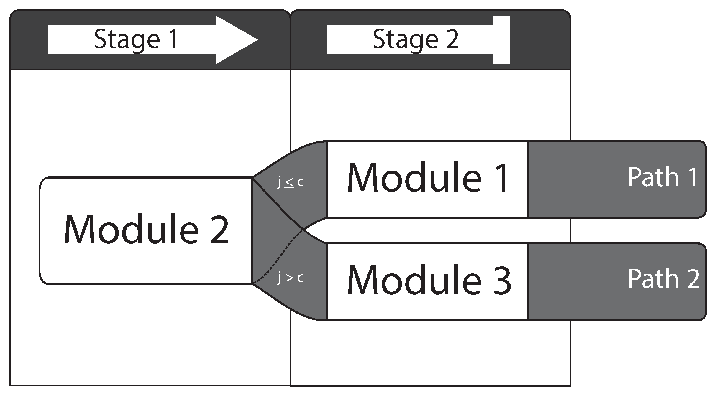
In MSTs, the decision points are modules. These are collections of items with mostly related content (see also the comparison to testlets; [6,38]), certain mean item difficulties, and variances. At the start, test persons receive a routing module and, based on the performance in this module and performance-related prior information, if available, one or more additional modules. Each additional module in this routing process describes a stage in the MST design. Each stage consists of at least two modules (see Figure 1 for an example). The specific combination of processed modules in the routing process is called a path. Different groups of modules, stages, and paths are called panels. Panels can be seen as parallel forms in LFTs. Routing in the MST context is branching from one to the next module, based on pre-specified rules.
As with all adaptive designs, the selection of items or modules is the central part of the design, and much research has been performed to serve different needs. In particular, in CATs, the item selection can become very complex. Additional considerations can refer to, e.g., content balancing or strategies to avoid overexposure and/or underexposure of items. Next to the desired purpose of that algorithm, there might also be some disadvantages, which can negatively impact the validity and the fairness of the test. In particular, in CATs, the item exposure control can become a challenging task [13,39].
Overexposure might be a problem if the information of those items processed more often is shared across test persons. This can threaten the validity of the test because the performance of the test persons can no longer be separable between ability and knowledge. Especially with high-stakes tests, it might be a major problem, where industry could quickly build up to collect the information of items [40]. While simply increasing the item pool is not the solution [39], additional algorithms must be considered. Concerning underexposure, economic considerations are probably more in the foreground, as the construction of items is very expensive. However, this can also lead to problems in parameter estimation if the sample size per item is low, which subsequently results in the inaccurate estimation of item parameters and the standard errors. Here, MST designs seem to show their advantages, as they can be designed and checked before they are applied. Hence, no additional algorithms are necessary.

1.1. Motivation

An essential factor in every test is the motivation of the test persons (see, e.g., [41,42,43]). It has been reported that due to the better match of the item difficulty and the person’s ability, test persons, especially those with low abilities, are more motivated to proceed, sometimes less bored, and more committed during the test [44,45,46,47,48,49,50]. On the other hand, there are several contributions concerning CATs that report negative psychological effects of the demanding item selection. Kimura [51] stated that this could lead to negative test experiences as well as lower motivation, lower self-confidence, and increased test anxiety (see also [52,53,54,55,56,57,58]). These psychological variables seem to be an important topic in testing since they could negatively affect the persons’ test performance [56,59,60]. Motivation is a key factor in every low-stakes test such as ILSAs since unmotivated participants might influence the test results and thus the validity of the test (see, e.g., [61]). It seems to be central and can be deduced from these contributions that the impact on motivation or boredom, but also anxiety, should not be ignored, as this can significantly influence the test results [62,63]. Finally, this contributes to standardization and thus to reliable results and more valid parameter estimates [64,65].
MST designs are conceptualized before the actual application. The items are explicitly assigned to modules, and every path of that design can be reviewed in advance. Therefore, these mentioned aspects can be verified before the application, and no additional algorithms are required during the actual application.

1.2. Test Anxiety

Increased test anxiety among test participants is another reported psychological effect in CATs [60]. Due to the lack of the possibility to review items that have already been processed and, if necessary, changed by the test person, test anxiety might also be further increased [66,67,68,69,70]. An item revision in CATs is not possible [7,71,72], because the item selection in CATs is based on the responses already given. Hence, changing responses retrospectively may impact the measurement precision, which results in larger standard errors [69,73,74,75,76,77,78]. Therefore, allowing item revision within CATs has been controversially discussed in the literature, even if some contributions encountered this measurement problem (see, e.g., [66,77,79,80,81,82]). While it can be argued that only a few persons might change their responses [83], a lack of this ability appears to contribute to increased test anxiety. However, it is also reported that subsequent changes to given responses are mostly from wrong to processed correct [83] and thus not only affect the psychological aspects, but also the validity of the test scores.
Several studies suggested methods to allow a (limited) item review in CATs while avoiding the negative effects of the lower measurement accuracy or the extension of the test at the same time [68,75,77,81,82,84]. However, the proposals can also be viewed critically. For example, Zwick and Bridgeman [85] found that more experienced test persons may use the review options more often than others. This could again harm the validity of the test, while the absence of the item review affects all persons across the entire skill range equally [60]. Next to the possibility of reprocessing the responses in CATs, this option can also be used to manipulate the test score [84,86]. Wainer [76] described one of these strategies, in which a test person first gives only incorrect responses to continuously obtain easier items. At the end of the test, all given responses are then corrected, which results in large measurement errors. Kingsbury [87] described a strategy in which test persons recognize whether a subsequent item is easier or more difficult than the one they have just worked on and obtain information about the given response. If the following item is easier, which hints that the prior response might be wrong, the response can be changed on this item; see also [88]. In MSTs, all test persons have the same chance to review their given responses and change them before taking on a new module. It is, therefore, to be expected that test anxiety will be lower with MSTs.

1.3. Routing in Adaptive Designs

Item selection algorithms are one of the key factors in CATs, especially when it comes to maximizing the test economy and thus shortening the test length [16]. Increasing the test efficiency can also be viewed critically, as we will discuss later. When choosing one of the selection algorithms, the optimization and the associated negative effects should be considered. Furthermore, the item selection is also related to considerations regarding under- and over-exposure, as well as considerations of the safety aspects. Some selection algorithms can be found in Chang [16].
In this context, deterministic means that persons with the same performance in the same module m [ b ] of B modules with b = ( 1 , , B ) in the same stage are routed to the same subsequent module. A decision base can be, e.g., the number of solved items (number-correct score; NC). Assuming a person θ p achieves a score j in the module m [ b ] , this person, given a cutoff value c, is routed to an easier module in the cases j < c or j c (that is, once again, performed deterministically by the test author) and, in the remaining cases, a more difficult module (see also [6,12]). In this simple case, the decision to route from one module to the next is only made based on the performance in the module currently being processed. This can easily be expanded by including the information from all previously processed modules in the decision. This type of routing should be referred to as the cumulative number-correct score (cNC; [89,90]). Since the information about the persons’ ability across modules is used, theoretically, a more valid routing is possible. In addition to the raw scores, the routing decision can also be made based on specifically processed items. Since item parameters are known, person parameters can be estimated a priori via the respective item combinations. This type of routing is referred to in the literature as item response theory (IRT)-based routing [91]. The decision for a routing strategy in MST is linked to the efficiency of the proposed design and can also impact the precision of item parameter estimation [6]. The available strategies can roughly be grouped into deterministic and probabilistic ones. Svetina et al. [89] compared different routing strategies. The authors concluded that the IRT-based routing performed best, but the NC-based routing was not significantly worse when it came to the median of person parameter recovery rates. An additional argument for NC-based routing is that it is much easier to implement.
In the mentioned probabilistic routing, the routing rule j < c , respectively j c , is expanded with an additional probability based on the performance j. This means that routing into an easier module is not solely based on the cutoff value c, but rather with a previously defined probability p , depending on the individual score j of person p. With the counter-probability 1 p and the same score j, the person is routed to a more difficult module. This type of routing is used, for example, in the PIAAC [32,92,93]. In addition to the deterministic definition of the cutoff values c, additional thresholds are defined for each decision stage and score.
A motivation to use probabilistic routing instead of exclusively deterministic is the possibility of being able to better control the exposure rate so that it is ensured across all proficiency levels that a minimum number of sufficient responses per item is guaranteed, even with difficult tasks (see, e.g., [32,93]).
To summarize: MSTs can be seen as a design with advantages from two perspectives. There are fully adaptive item-by-item designs such as CATs with a very high test economy [14,23,94], on the one hand, and LFTs, on the other [94]. MSTs allow for more efficient testing; test persons can review items within modules they have already worked on and change their responses if necessary. The design can be examined by the test authors concerning the item content regarding content balancing and security concerns, but also possible differential item functioning. Even overexposure and underexposure can be controlled more easily [95]. While CATs are tied to the computer, MSTs can also be administered as paper-pencil tests [19,22,30].

2. Item Parameter Estimation

Item parameter estimation in adaptive designs is an important topic and relates to the MST’s main component of this contribution. For the calibration of an item pool, with data obtained by an MST, an item response theory model such as the Rasch model (1PL; [96]) is fitted. Item parameters are typically regarded as fixed, and persons are treated as either fixed or random (see, e.g., [9,97,98,99,100], for a further discussion on this topic). Several methods are available, which will be briefly discussed in the following.
These are the marginal maximum likelihood method (MML; [101,102,103]) and the conditional maximum likelihood method (CML; [104,105]). Various considerations can lead to choosing one of these estimation methods, such as the flexibility of that approach or more fundamental beliefs about the method.
The MML estimation method can also be applied in MST designs without leading to biased item parameter estimates (see, e.g., [106,107,108]). The CML-based parameter estimation in MSTs, without severely biased item parameter estimates [108], is only feasible by modifying the CML estimation method proposed by Zwitser and Maris [109]. Besides the relatively newly proposed modification of the CML approach, the normal MML method and models with non-normal trait [110] are available. It is frequently argued that the CML estimation method enables the estimation of item parameters independent of the distribution assumptions of the trait [107,108,109,111]. Comparisons between CML and MML estimation in MSTs showed biased item parameter estimates in MML if the distribution assumption deviates severely from the true distribution (see, e.g., [109]). In our contribution, the estimation methods were systematically examined and compared. In this context, it seems very interesting that scaling the data using a multigroup model, in which the groups are represented by the respective paths in the MST design, seems to lead to severely biased parameter estimates [106].
In the following, we only considered dichotomous item responses and utilized the 1PL model. In the 1PL model, the probability of solving item i with difficulty β i by person p with ability θ p can be expressed as:
P ( X p i = x p i θ p , β i ) = exp [ x p i ( θ p β i ) ] 1 + exp ( θ p β i ) ,
with x p i = 1 . Then, the likelihood L ( x p θ p , β ) with responses x p = ( x p 1 , x p 2 , , x p I ) of the test person p with ability θ p and the item difficulty β = ( β 1 , β 2 , , β I ) can be expressed as follows:
L ( x p θ p , β ) = exp ( r p θ p i = 1 I x p i β i ) i = 1 I ( 1 + exp ( θ p β i ) )
with r p as the raw score of person p with r p = i = 1 I x p i . Equation (2) can be seen as the starting point for the following approaches in parameter estimation. The likelihood for the response matrix X can be expressed as:
L ( X θ , β ) = exp ( p = 1 P r p θ p p = 1 P i = 1 I x p i β i ) p = 1 P i = 1 I ( 1 + exp ( θ p β i ) )

2.1. Marginal Maximum Likelihood Estimation

For the estimation in the parametric case (see Equation (4)), a distribution G with probability density function g ( θ ; α ) with a vector α containing the parameters of the latent ability distribution is introduced for person parameter θ . It is assumed that the persons are a random sample from this population, e.g.,  θ N ( μ , σ 2 ) . The random variable θ is integrated out of the marginal log-likelihood function. For parameter estimation in MST designs, Glas [108] and Zwitser and Maris [109] stated that the distributional assumptions could be incorrect, and the estimated item parameter estimates can be severely biased. Therefore, the following simulation should shed some light on this.
Data collected based on the MST design have missing values due to the design. Mislevy and Sheehan [112], referring to Rubin [113], showed that MML provides consistent estimates in incomplete designs in general (see also [106]). For MST designs, it can be shown that MML can also be applied to MST, following this justification [106,109]. Based on the likelihood function (3), in the MML case, the likelihood for the observed data matrix X is the product of the integrals of the respective likelihood of the response patterns x i .
L M M L ( X β , μ , σ 2 ) = r = 0 I exp ( r θ i = 1 I s i β i ) i = 1 I ( 1 + exp ( θ β i ) ) g ( θ ; α ) d θ n r
with s i = p = 1 P x p i the item score of item i, n r as the number of test persons with the raw score r, and α as a parameters for the distribution G .
For model identification purposes, if a normal distribution is assumed, the mean is fixed to zero μ = 0 , and  σ 2 is freely estimated. Therefore, the marginal likelihood is no longer dependent on θ (see Equation (4)). The integral in Equation (4) can be solved by, e.g., Gauss–Hermite quadrature by summing over a finite number of discrete quadrature points θ q with q = ( 1 , , Q ) and the corresponding weights w q = w q (see, e.g., [101,102]).
L M M L ( X β , G ) = r = 0 I exp ( i = 1 I s i β i ) q = 1 Q exp ( r θ q ) i = 1 I ( 1 + exp ( θ q β i ) ) w q n r

Marginal Maximum Likelihood with Log-Linear Smoothing

For the specification of the unknown latent ability distribution G in Equation (4), both parametric and nonparametric strategies are available. Another interesting approach for the specification, which is flexible and parsimonious in terms of the number of parameters to be estimated, is the application of log-linear smoothing (LLS; [110,114,115]). In IRT, this method was used, for example, by Xu and von Davier [110]. They fitted an unsaturated log-linear model in the framework of a general diagnostic model (GDM; [116]) to determine the discrete (latent) ability distribution g ( θ ) . The LLS model used here in the case of the 1PL can be described as log w q δ 0 + m = 1 M δ m w q m [115,117]. Here, log w q describes the logarithmic weighted quadrature points ( θ 1 , , θ Q ) . The intercept δ 0 is a normalization constant, M the moments to be fitted, and δ m the dependent coefficients to be estimated. The central property of log-linear smoothing is the matching of the moments of the empirical distribution.
An interesting connection between the MML parameters’ estimation outlined above in Section 2.1 using a nonparametric approach as described by Bock and Aitkin [101] (also referred to as a Bock–Aitkin or the empirical histogram (EH) solution) and the LLS is that the former can be seen as a special case of the LLS method with M = Q 1 moments.
The LLS is integrated into the EM algorithm [110] to estimate β since the number of expected persons (expected frequencies) at each quadrature point g q is unobserved. An LLS with M = 2 moments is equivalent to a discretized (standard) normal distribution (exactly two parameters are necessary, μ and σ 2 ) (see [117]). The specification of more than two moments allows, e.g., the specification of skewed latent variables [118].
Casabianca and Lewis [115] showed in detailed and promising simulation studies that the LLS method leads to better parameter recovery if the specified distribution deviates from the true empirical ones. By specifying up to four moments, bimodal distributions could be captured. It is also worth mentioning that there may be less effort for users to use this method since only the number of moments has to be specified.

2.2. Conditional Maximum Likelihood Estimation

Unlike the MML method, CML does not require assumptions for the distribution of the traits. Here, the person parameter is eliminated from the likelihood due to conditioning on the raw scores r p , which is referred to as minimal sufficient statistic for person parameter θ p [96,104,105,119] in Equation (6). Therefore, only item parameters β i , but no person parameter θ p , are estimated, which have to be determined afterwards. In the following, the likelihood for the response matrix X in the CML case is outlined following Equation (3) again.
For the estimation of item parameter, the calculation of the elementary symmetric function (ESF) γ ( r , β ) of order r p of β 1 , β 2 , , β I is the crucial part of the likelihood in CML. Different methods have been proposed, which differ mainly in accuracy and speed [120,121,122].
There are I r p different possibilities to obtain the score r p for a person with the ability θ p . The sum over these different possibilities results in γ ( r , β ) = x i x i = r exp ( i = 1 I x i β i ) , with given item difficulty β i , as well as the responses x i for a given score r.
L C M L ( X r , β ) = L ( X θ , β ) L ( r β )
The likelihood of the response vector r can be written as:
L ( r β ) = exp ( p = 1 P r p θ p ) p = 1 P x p i r p exp ( i = 1 I x p i β i ) p = 1 P i = 1 I ( 1 + exp ( θ p β i ) )
The likelihood in Equation (6) can then be written using Equations (3) and (7) in the CML case as follows:
L C M L ( X r , β ) = exp ( i = 1 I s i β i ) r = 0 I γ ( r , β ) n r
The resulting estimates β ^ are consistent, asymptotically efficient, and asymptotically normally distributed [99].

CML Approach of Zwitser and Maris (2015)

Glas [108] stated that ignoring the MST design in the CML item parameter estimation process leads to severely biased estimates (see also [107,111]). Based on these results, it has long been recommended not to use the CML method for MST designs. The MML method offered an alternative, or the parameter of the items for each path or module could be estimated separately using the CML method [123]. The latter has the major disadvantage that item parameters estimated in this way can no longer be compared. Recently, this CML estimation problem could be solved for deterministic routing while considering the respective MST design in the CML estimation process [109]. To solve this problem, the symmetric function has to be modified, such that only those raw scores are considered, which can occur due to the specific MST design. This leads to consistent item parameter estimates. There are currently two R [124] packages for this method: dexterMST [125] and tmt [126]. The modified CML estimate is outlined in the following. In the deterministic case, a person with score j is routed from one module m [ b ] to the next module based on a cut-score c. Based on the design in Figure 1, the probability of reaching a score of x [ 1 , 2 ] in the modules m [ 1 , 2 ] with ability θ , and the number of solved items in the module m [ 1 ] being less than or equal to the cut-score c with X + [ 1 ] c , can be described as follows:
P m [ 1 , 2 ] ( x [ 1 , 2 ] θ , X + [ 1 ] c ) = P m [ 1 , 2 ] ( x [ 1 , 2 ] , X + [ 1 ] c θ ) P m [ 1 , 2 ] ( X + [ 1 ] c θ ) = P m [ 1 , 2 ] ( x [ 1 , 2 ] θ ) P m [ 1 , 2 ] ( X + [ 1 ] c θ )
The ESF as described above can be written as γ s ( m [ b ] ) = x : x + [ b ] = s i exp ( x i [ b ] β i [ b ] ) and rearranged as γ x + ( m ) = i + j + k = x + γ i ( m [ 1 ] ) γ j ( m [ 2 ] ) γ k ( m [ 3 ] ) . Here, the ESF is first evaluated for each module separately and then for a specific path of the MST design. Zwitser and Maris [109] proposed to partition the denominator of the likelihood into the sum of items j = 0 , , c in the first module and x + [ 1 , 2 ] j items in the second module. Equation (9) can be factored as:
P m [ 1 , 2 ] ( x [ 1 , 2 ] θ , X + [ 1 ] c ) = P m [ 1 , 2 ] ( x [ 1 , 2 ] x + [ 1 , 2 ] , X + [ 1 ] c ) P m [ 1 , 2 ] ( x + [ 1 , 2 ] θ , X + [ 1 ] c )
Inserting Equation (10) into the common CML approach results in:
P m [ 1 , 2 ] ( x [ 1 , 2 ] x + [ 1 , 2 ] ) = i exp ( x i [ 1 ] β i [ 1 ] ) j exp ( x j [ 2 ] β j [ 2 ] ) j = 0 n [ 1 , 2 ] γ j ( m [ 1 ] ) γ x + [ 1 , 2 ] j ( m [ 2 ] )
The probability of X + [ 1 ] being less than or equal to c conditional on x + [ 1 , 2 ] :
P m [ 1 , 2 ] ( X + [ 1 ] c x + [ 1 , 2 ] ) = j = 0 c γ j ( m [ 1 ] ) γ x + [ 1 , 2 ] j ( m [ 2 ] ) j = 0 n [ 1 , 2 ] γ j ( m [ 1 ] ) γ x + [ 1 , 2 ] j ( m [ 2 ] )
Following Equations (11) and (12), we obtain:
P m [ 1 , 2 ] ( x [ 1 , 2 ] x + [ 1 , 2 ] , X + [ 1 ] c ) = P m [ 1 , 2 ] ( x [ 1 , 2 ] , X + [ 1 ] c x + [ 1 , 2 ] ) P m [ 1 , 2 ] ( X + [ 1 ] c x + [ 1 , 2 ] ) = P m [ 1 , 2 ] ( x [ 1 , 2 ] x + [ 1 , 2 ] ) P m [ 1 , 2 ] ( X + [ 1 ] c x + [ 1 , 2 ] ) = i exp ( x i [ 1 ] β i [ 1 ] ) j exp ( x j [ 2 ] β j [ 2 ] ) j = 0 c γ j ( m [ 1 ] ) γ x + [ 1 , 2 ] j ( m [ 2 ] )
and further:
P m [ 1 , 2 ] ( x + [ 1 ] , x + [ 2 ] θ ) = γ x + [ 1 ] ( m [ 1 ] ) γ x + [ 2 ] ( m [ 2 ] ) exp ( x + [ 1 ] + x + [ 2 ] ) θ 0 j + k n [ 1 , 2 ] γ j ( m [ 1 ] ) γ k ( m [ 2 ] ) exp ( j + k ) θ
Taking the same considerations from Equation (14) for the following:
P m [ 1 , 2 ] ( x + [ 1 , 2 ] θ , X + [ 1 ] c ) = P m [ 1 , 2 ] ( x + [ 1 , 2 ] , X + [ 1 ] c θ ) P m [ 1 , 2 ] ( X + [ 1 ] c θ ) = j c γ j ( m [ 1 ] ) γ x + [ 1 , 2 ] j ( m [ 2 ] ) exp ( x + [ 1 , 2 ] ) θ 0 j + k n [ 1 , 2 ] j c γ j ( m [ 1 ] ) γ k ( m [ 2 ] ) exp ( j + k ) θ
then it follows that:
P m [ 1 , 2 ] ( x [ 1 , 2 ] θ ) = P m [ 1 ] ( x [ 1 ] x + [ 1 ] ) P m [ 2 ] ( x [ 2 ] x + [ 2 ] ) P m [ 1 , 2 ] ( x + [ 1 ] , x + [ 2 ] x + [ 1 , 2 ] ) P m [ 1 , 2 ] ( x + [ 1 , 2 ] θ )
Using Equations (13), (15) and (16), Equation (10) follows. Therefore, it can be concluded that after the integration of additional design information in the MST design, the CML item parameter estimation is justified.

3. Simulation Study

A Monte Carlo simulation was carried out to provide information on the influence of different trait distributions on the estimation of item parameters in MST designs. In addition to the different trait distributions (normal, bimodal, skewed, and  χ 2 with d f = 1 ), the test length (I = 15, 35, and 60 items), different MST designs, and sample sizes (N = 100, 300, 500, and 1000) were considered. All conditions were simulated as MSTs, as well as fixed-length tests. The simulation and all conditions are explained in detail below. MST designs can be expanded to more modules, items within modules, and more stages. It is important to note that, branching on the item level as is the case with CATs, CML estimation is not possible. As stated by Zwitser and Maris [109] for CATs, the information about the item parameters is bound in the design and thus not available for CML parameter estimation. Therefore, CAT designs were not considered here.

3.1. Data Generation

For all MST conditions, a two-stage design was used (see Figure 1). All MST conditions started with the routing module m [ 2 ] and were subsequently routed in one additional module. The module with easier items was the module m [ 1 ] and the module with more difficult items m [ 3 ] . The entire routing was based on the NC score. We chose deterministic routing for all multistage conditions because no additional random aspects influenced the routing process. The routing module in the test length condition I = 15 and I = 35 contained five items. The routing model in the condition with I = 60 contained ten items. The cutoff values for the routing into module m [ 1 ] within the first two conditions were j 2 and for the third condition j 5 . Item parameters of all models were drawn from a uniform distribution U ( 2 , 2 ) , whereby the item parameters for the routing module m [ 2 ] were from U ( 1 , 1 ) , m 1 from U ( 2 , 1 ) , and  m [ 3 ] from U ( 1 , 2 ) . In the simulation, four different types of (standardized) distribution of g ( β ) were considered (see Figure 2; skew as skewness and kurt as the kurtosis parameter):
(a)
(standard) normal ( s k e w = 0 , k u r t = 0 ): θ N ( 0 , 1 ) ;
(b)
bimodal ( s k e w = 0.3 , k u r t = 1.0 ): θ 3 5 N ( 0.705 , 0.254 ) + 2 5 N ( 1.058 , 0.254 ) ;
(c)
skewed ( s k e w = 1.5 , k u r t = 3.2 ): θ 1 5 N ( 1.259 , 1.791 ) + 4 5 N ( 0.315 , 0.307 ) ;
(d)
χ 1 2 ( s k e w = 2.8 , k u r t = 12 ): θ χ 1 2 with one degree of freedom.
The skewed and bimodal distribution parameters were chosen following Casabianca and Lewis [115]. This study also dealt with parameter recovery for MML with log-linear smoothing, but solely in LFT designs. The authors reported that they chose theses parameter based on their own work [127], as well as other contributions that also dealt with simulation studies on the same or related topics (see, e.g., [128,129,130,131,132,133]).
In disciplines such as educational measurement, clinical psychology, or medicine, there are many situations where the resulting trait distribution might deviate from an assumed normal distribution (see, e.g., [115,129,132,134,135]). A bimodal trait distribution might occur, e.g., in clinical and personality psychology, if one aspect of personality or psychopathology is low for most people and a few people high. One such reported dimension is, e.g., psychoticism, which tends to be positively skewed towards low scores [136]. Furthermore, in situations where groups of persons are examined, in which a subgroup has psychopathological symptoms, distributions deviating from a normal distribution are expected and typically positively skewed [137]. Areas of (large-scale) educational testing, as well as raw scores of state-wide tests tend to be non-normal distributed [138,139].
A bimodal distribution can be expected when two different groups of examinees are investigated, e.g., high versus low performer or schools with privileged versus underprivileged students [140].
For the estimation, the following three different estimation approaches were used:
  • CML/CMLMST: CML estimation with consideration of the respective MST design in the MST condition (CMLMST);
  • MMLN: MML estimation, assuming that traits are normally distributed;
  • MMLS: MML estimation with log-linear smoothing up to four moments.
For each condition, 1000 datasets were generated, and the CML and MML estimation methods were applied. Thereby, 1000 replications R were conducted in each cell. For the parameter estimation and the analysis of the simulation study, the open-source software R [124] was used. For reasons of the comparability of the estimated item parameters across the different estimation methods, the estimated item parameters were centered after estimation.

3.2. Implementation in R

All introduced estimation methods were implemented in R packages. For the conventional CML estimation, there is a wide variety of packages available. In addition to the well-known eRm with eRm::RM() [141], these are, for example, the R packages with the respective functions psychotools with psychotools::raschmodel(), immer with immer::immer_cml() and tmt with the function tmt::tmt_rm(), to name a few representatives [126,141,142,143]. All packages allow a user-friendly application, but they differ in terms of speed and the availability of further analysis options. With regard to CML parameter estimation in MST designs, two packages are currently available: dexterMST with dexterMST::fit_enorm_mst() and tmt with the function tmt::tmt_rm(). The two packages differ concerning the specification of the MST design to be taken into account. In dexterMST, first, an MST project must be created with the function dexterMST::create_mst_project(), then the the scoring rules used with dexterMST::add_scoring_rules_mst() are handed over. Essentially, this is a list of all items, admissible responses, and assigned scores to each response when grading. For the estimation, the routing rules were set with dexterMST::mst_rules() and with dexterMST::create_mst_test(), then the actual test was carried out, created from the specified rules and the defined modules. Once these steps were executed, the actual data were added with dexterMST::add_booklet_mst() to the created database. The actual parameter estimation was realized with dexterMST::fit_enorm_mst(). Furthermore, in the tmt package, the actual used MST design must be defined. For this purpose, a model language was developed that could be used to define the modules and routing rules. In the first section, the modules were defined, in the example below indicated as m1, m2 and m3. Subsequently, each path of the MST design with the respective rules was specified (in the example below with p1 and p2). In deterministic routing, the lower and upper limit of the raw scores must be specified for each module in each path. The parameter estimation was realized with tmt::tmt_rm() with the specified design as an additional argument.
model <- “
m1 =~c(i01,i02,i03,i04,i05)
m2 =~c(i06,i07,i08,i09,i10)
m3 =~paste0(’i’,11:15)
p1 := m2(0,2) + m1
p2 := m2(3,5) + m3
Furthermore, for MML parameter estimation, numerous packages are available. Some selected examples are ltm with ltm::rasch(), sirt with sirt::rasch.mml2() and TAM with TAM::tam.mml() or mirt with mirt::mirt(), which also differ in functionality and speed [144,145,146,147]. In contrast to CML estimation, no further steps were necessary to obtained the unbiased estimates. The log-linear smoothing used here is available in the package sirt [145]. As already pointed out positively by Casabianca and Lewis [115], only the desired number of moments needs to be specified additionally. This can also be emphasized as an advantage compared to the described CML estimation in MST designs, especially in cases with complex MST designs. To utilize the log-linear smoothing, the package sirt with the function sirt::rasch.mirtlc() is available. The model type (in our case, modeltype = “MLC1”) and the trait distribution distribution.trait = “codesmooth4” were passed as an additional argument (in this example, up to four moments). In the simulation described here, we utilized the R package sirt [145] for MML estimation and the R package tmt [126] for CML estimation.

3.3. Outcome Measures

To compare the different estimation methods under the different simulation conditions, we computed three criteria. The focus was the estimated item parameters β ^ in each simulation condition. The computed quantities were the bias of the estimates, the accuracy measured with the root mean squared error (RMSE), and the average relative RMSE (RRMSE) as a summary of the bias and variability. The bias represents the absolute deviation of item parameter estimates from the true item parameter and is reported as the average absolute bias (ABIAS) overall replication in each condition.
A B I A S ( β ^ ) = 1 I i = 1 I 1 R r = 1 R β ^ i r β i = 1 I i = 1 I B i a s ( β ^ i )
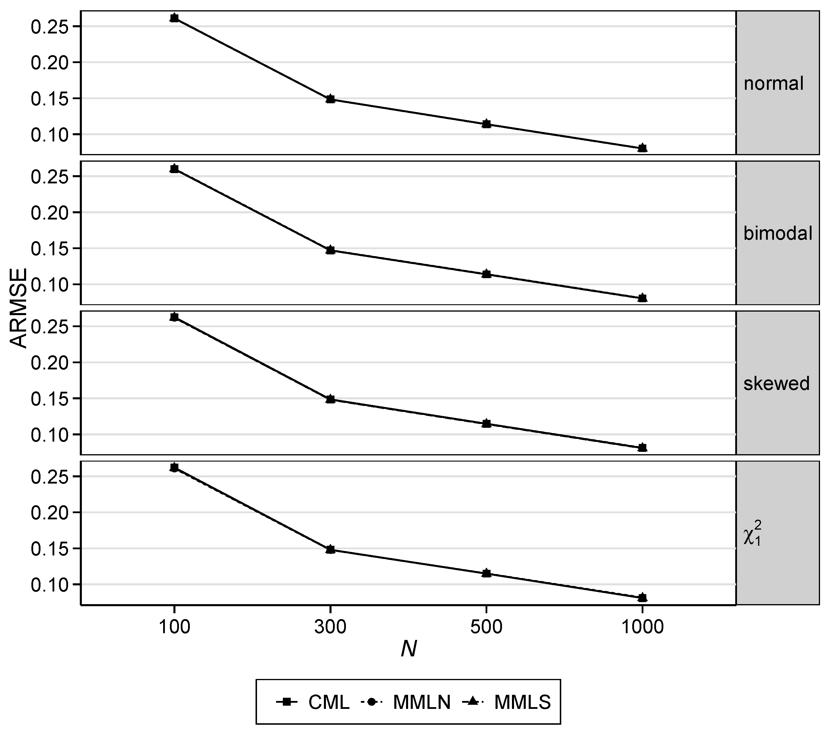
For the evaluation of the overall accuracy of item parameter estimation, the RMSE was computed. The average RMSE was calculated as the square root of the squared differences between the estimated and true item parameters. The ABIAS and the ARMSE are reported, each as the average for each condition and in the MST case for each module separately.
A R M S E ( β ^ ) = 1 I i = 1 I 1 R r = 1 R ( β ^ i r β i ) 2 = 1 I i = 1 I R M S E ( β ^ i )
The RRMSE is defined as follows:
R R M S E ( β ^ ) = i = 1 I R M S E ( β ^ i ) i = 1 I S D r e f e r e n c e ( β ^ i ) ,
where S D r e f e r e n c e is the average standard deviation of the item parameters of the CML method in the fixed-length condition, respectively CMLMST in the MST condition, and serves hereby as the reference.

4. Results

The results of the simulation study are reported separately for the conditions of the LFT and MST. In both conditions, the RMSE is reported in the figures and the ABIAS and RRMSE in the tables. In the simulation, there were no items that all persons did not or wholly solved. Concerning the persons who solved all items or none of the items, the average was 2.5 % in the fixed-length condition and 2.6 % in the multistage condition. We did not exclude any persons in this regard, but used the default settings of the respective packages. For the item parameter estimation, this was neither a problem for the CML nor the MML estimation method (see, e.g., [148]).

4.1. Results for the Linear Fixed-Length Test Condition

The results for the LFT showed across the estimation conditions very minor differences. Therefore and for a better overview, only the results for the long test condition ( I = 60 ) are presented (results for all test lengths and sample sizes can be found in Appendix A Table A1). In Figure 3, the RMSE of all estimation conditions decreased across all trait distribution conditions. There was no difference between the estimation methods either in the normal or in the non-normal conditions (bimodal, skewed, χ 1 2 ).
The ABIAS and RRMSE reported in Table 1 show very similar results. In the normal distribution condition, there was no difference between the different estimation methods concerning the BIAS of the item parameters. With large sample sizes ( N = 1000 ), the MMLS method seemed to lead to a slightly smaller RRMSE compared to CML and MMLN. In the conditions of non-normal distribution, the results were more heterogeneous. In the bimodal condition, the MMLN method with a small sample size ( N = 100 ) led to smaller bias, but the difference to CML and MMLS decreased with increasing sample size. The ABIAS in the conditions skewed and χ 1 2 was lower in the CML method, but the difference between CML and MMLS decreased with increasing sample size. It is noteworthy that in the condition skewed, the difference between CML and MMLS was lower than in the condition χ 1 2 : here, the CML method led to a smaller bias of the item parameters even with larger sample sizes. Regarding the RRMSE, the MMLS led in both the bimodal, as well as the skewed condition for medium and large sample sizes to the smallest RRMSE. In the χ 1 2 condition, both the CML and MMLS method led to lower RRMSE compared to MMLN. However, it can be summarized that even for the MMLN approach, the results showed compared to the CML and also MMLS condition that the misspecification of the trait distribution had no (large) influence (see also [149]) for a more detailed discussion on different trait distributions in the LFT.

4.2. Results for the Multistage Test Condition

The results for the MST condition were more differentiated and therefore discussed separately. For a better overview, the results are not reported separately by module; these can be found in the Appendix A in Figure A1 for the RMSE and two separate tables for the ABIAS in Table A2 and the RRMSE in Table A3. The RMSE in Figure 4 indicates that the conventional CML estimate (i.e., the CML method without considering the respective MST design) led to the largest RMSE across all conditions.

4.2.1. Normal Distribution

In Figure 4, the RMSE in the condition with a normal trait distribution was the smallest for the MMLN method. This result was expected because this was the condition with the correct distribution specification. The difference between the estimation methods was small. Concerning the test lengths and sample size, the RMSE of the MMLN method was smaller for short and medium test lengths ( I = 15 , 35 ) and small sample sizes, but vanished for longer test lengths or sample sizes above N = 300 . Overall, the difference between the estimation methods in the condition normal distribution except for the CML method seemed to be quite low. With regard to the relative RMSE (RRMSE) in Table 2 at which all estimation methods were referenced to the CMLMST method, these results can be confirmed. Relating to ABIAS, the CMLMST method led to a smaller average bias of the item parameters; however, the difference between CMLMST and MMLN was very small, especially for sample sizes above N = 100 .

4.2.2. Non-Normal Distributions

In the conditions with a non-normal trait distribution, the MMLN method led nearly in all conditions to a higher RRMSE compared to CMLMST and MMLS. Exceptions were the bimodal condition with a small sample size ( N = 100 ) together with a short to medium test length ( I = 15 , 35 ) and the χ 1 2 condition with a long test length ( I = 60 ). It should be emphasized that in all other non-normal distribution conditions, the MMLS method led to smaller RRMSE regardless of the sample size and test length compared to MMLN and CMLMST. Concerning the bias of the item parameter in Table 2, the CMLMST method showed the smallest ABIAS independently of sample size and test length. In the bimodal distribution condition, the difference between CMLMST and MMLS was comparatively small, but it should be noted that it was also smaller for the MMLS condition compared to CMLMST. Concerning the two other non-normal distribution conditions (skewed, χ 1 2 ), the bias of the item parameter in the CMLMST was smaller regardless of sample size and test length.

5. Summary and Discussion

For the estimation of item parameters, alternative estimation methods are available.
While users of the CML method often emphasize that this method comes close to the idea of person-free assessment [148] required for the postulation of specific objectivity [150,151] and that no distribution assumption for the person parameters are required, supporters of the MML method might highlight the flexibility of the approach.
When it comes to MST designs, there was only MML estimation available. If CML parameter estimation were applied, the estimated item parameters would be severely biased. Based on the contribution by Zwitser and Maris [109], two implementations in R packages dexterMST [125] and tmt [126] are available for item parameter estimation using the CML method in MST designs.
The simulation study was carried out to investigate the influence of trait distributions on the estimation of item parameters. The results showed a differentiated picture. As the sample size increased and the number of items increased, the CMLMST method showed a comparatively small RMSE. As expected, the MMLN method led to a comparatively large RMSE in all non-normal distribution conditions. It is noteworthy that the MMLS estimation method provided the smallest RMSE across conditions. The results were very similar between MMLS and CMLMST, especially with increasing sample sizes and an increasing number of items, even though the MMLS method objectively led to a smaller RMSE. Based on the results, it seems favorable for MST designs to either use the CMLMST or MMLS estimation. Concerning the bias of the item parameter, the CMLMST method led to the smallest ABIAS independently of sample size and test length in nearly all MST conditions. However, in the decision for the CMLMST or MMLS method, it should be considered that the actual distribution used in the MMLS method was assumed to resemble the true population distribution, which may differ. This might be an advantage of the CMLMST method since no distribution assumption was made here.
There are also limitations associated with the present study that might limit the generalizability of the findings. In our research question, we were interested in the influence of the type of trait distribution on item parameter estimation. The number of items and the MST design were varied as additional factors. It would be interesting to systematically study the impact of using more complex MST designs in further studies and perhaps also consider Bayesian estimation methods (see, e.g., [152]). It was noticeable in the results that for the 60-item condition with a χ 1 2 trait distribution, the difference in the RMSE among CML, MMLN, and MMLS was smaller than in the two other item conditions (15 and 35). Next to the different number of items, the MST design in the condition with 60 items differed in the size of the routing module with ten instead of five items. On the other hand, the difference between CML and MMLN seemed to increase with an increasing number of items, but the same size of the routing module. Therefore, it would be interesting to investigate more complex MST designs for item parameter estimation in future research.

Author Contributions

Conceptualization, J.S. and A.R.; methodology, J.S. and A.R.; software, J.S.; validation, J.S. and A.R.; formal analysis, J.S.; investigation, J.S.; writing—original draft preparation, J.S.; writing—review and editing, J.S. and A.R.; visualization, J.S. and A.R.; supervision, A.R.; project administration, J.S. All authors have read and agreed to the published version of the manuscript.

Funding

This research received no external funding.

Institutional Review Board Statement

Not applicable.

Informed Consent Statement

Not applicable.

Data Availability Statement

The script for the simulation presented are available on request from the corresponding author.

Acknowledgments

We would like to thank the two anonymous reviewers for their careful reading, comments, and suggestions, which led to an improved final manuscript.

Conflicts of Interest

The authors declare no conflict of interest.

Abbreviations

The following abbreviations are used in this manuscript:
1PLone-parameter logistic model
ABIASaverage absolute bias
ARMSEaverage root mean squared error
CATcomputerized adaptive tests
CMLconditional maximum likelihood
CMLMSTCML estimation with consideration of the respective MST design
cNCcumulative number-correct score
ESFelementary symmetric function
GDMgeneral diagnostic model
ILSAsInternational Large-Scale Assessments
IRTitem response theory
LFTlinear fixed-length test
LLSlog-linear smoothing
MMLmaximum likelihood method
MMLNMML estimation, assuming that traits are normally distributed
MMLSMML estimation with log-linear smoothing up to four moments
MSTmultistage test
NAEPNational Assessment of Educational Progress
NCnumber-correct score
PIAACProgramme for the International Assessment of Adult Competencies
PISAProgramme for International Student Assessment
RMSEroot mean squared error
RRMSErelative root mean squared error
TIMSSTrends in the International Mathematics and Science Study

Appendix A

In Table A1, the results for all test lengths and sample sizes for the linear fixed-length test condition are reported. The results for the multistage condition separately by module and in total can be found in Figure A1 for the RMSE, in Table A2 for the ABIAS, and in Table A3 for the RRMSE.
Table A1. Average absolute bias (ABIAS) and relative root mean squared error (RRMSE) for the fixed-length test condition as a function of sample size N and the number of items I for each trait distribution.
NormalBimodalSkewed χ 1 2
CriterionNICMLMMLNMMLSCMLMMLNMMLSCMLMMLNMMLSCMLMMLNMMLS
ABIAS100150.0170.0160.0170.0210.0190.0210.0200.0280.0200.0200.0320.021
350.0170.0170.0180.0180.0140.0180.0190.0250.0200.0220.0310.023
600.0180.0180.0180.0170.0150.0180.0200.0250.0210.0210.0270.022
300150.0050.0050.0050.0050.0060.0050.0070.0190.0070.0060.0240.006
350.0080.0080.0080.0080.0060.0080.0070.0150.0070.0080.0190.010
600.0080.0080.0080.0080.0060.0080.0060.0120.0070.0070.0150.009
500150.0030.0030.0030.0040.0070.0040.0030.0190.0030.0040.0240.005
350.0050.0050.0040.0050.0040.0050.0050.0130.0050.0040.0160.006
600.0040.0040.0040.0040.0030.0040.0050.0110.0050.0050.0130.007
1000150.0020.0020.0020.0030.0080.0020.0020.0180.0030.0030.0240.003
350.0020.0020.0020.0030.0050.0030.0030.0120.0030.0030.0160.005
600.0020.0020.0020.0030.0030.0030.0030.0090.0030.0030.0120.005
RRMSE10015100.2100.1100.2100.4100.5100.5100.499.8100.1100.499.6100.1
35100.2100.2100.2100.3100.4100.3100.399.9100.0100.499.8100.1
60100.2100.2100.3100.2100.4100.3100.3100.1100.2100.399.9100.1
30015100.099.999.9100.1100.3100.0100.1100.599.7100.1100.899.8
35100.1100.1100.0100.1100.3100.0100.1100.199.7100.1100.3100.0
60100.1100.1100.1100.1100.3100.1100.1100.099.8100.1100.0100.0
50015100.0100.099.9100.0100.599.9100.0101.299.6100.1102.099.9
35100.1100.099.9100.1100.399.9100.1100.499.6100.0100.599.9
60100.1100.1100.0100.0100.299.9100.1100.199.8100.1100.2100.1
100015100.0100.099.8100.0100.899.8100.0102.799.6100.0104.8100.0
35100.0100.099.8100.0100.599.8100.0100.999.6100.1101.9100.0
60100.0100.099.9100.1100.299.9100.0100.499.7100.0100.8100.1
Note: ABIAS = average absolute bias; RRMSE = relative root mean squared error with CML as reference; normal = (standard) normal ( s k e w = 0 , k u r t = 0 ): θ N ( 0 , 1 ) ; bimodal ( s k e w = 0.3 , k u r t = 1.0 ): θ 3 5 N ( 0.705 , 0.254 ) + 2 5 N ( 1.058 , 0.254 ) ; skewed ( s k e w = 1.5 , k u r t = 3.2 ): θ 1 5 N ( 1.259 , 1.791 ) + 4 5 N ( 0.315 , 0.307 ) ; χ 1 2 ( s k e w = 2.8 , k u r t = 12 ): θ χ 1 2 with one degree of freedom. All distributions are transformed such that E ( θ ) = 0 and Var ( θ ) = 1 . CML = conditional maximum likelihood; MMLN = marginal maximum likelihood estimation (MML) with normal distribution; MMLS = MML with log-linear smoothing up to four moments.
Figure A1. Average root mean squared error (ARMSE) for the multistage condition as a function of sample size N and the number of items for each module separately and in total for each trait distribution. Note: ARMSE = average root mean squared error; normal = (standard) normal ( s k e w = 0 , k u r t = 0 ): θ N ( 0 , 1 ) ; bimodal ( s k e w = 0.3 , k u r t = 1.0 ): θ 3 5 N ( 0.705 , 0.254 ) + 2 5 N ( 1.058 , 0.254 ) ; skewed ( s k e w = 1.5 , k u r t = 3.2 ): θ 1 5 N ( 1.259 , 1.791 ) + 4 5 N ( 0.315 , 0.307 ) ; χ 1 2 ( s k e w = 2.8 , k u r t = 12 ): θ χ 1 2 with one degree of freedom. All distributions are transformed such that E ( θ ) = 0 and Var ( θ ) = 1 . CML = conditional maximum likelihood (CML); CMLMST = CML estimation with consideration of the respective MST design; MMLN = marginal maximum likelihood estimation (MML) with normal distribution; MMLS = MML with log-linear smoothing up to four moments.
Psych 03 00022 g0a1
Table A2. Average absolute bias (ABIAS) for the multistage condition as a function of sample size N and the number of items I for each module separately and in total for each trait distribution.
NormalBimodalSkewed χ 1 2
NIModulesCMLMSTCMLMMLNMMLSCMLMSTCMLMMLNMMLSCMLMSTCMLMMLNMMLSCMLMSTCMLMMLNMMLS
10015m10.0310.5740.0370.0440.0270.5250.0310.0250.0280.6410.0700.0480.0340.6250.1350.042
m20.0100.0810.0100.0110.0100.0810.0150.0090.0160.0950.0510.0190.0130.0910.0720.008
m30.0280.5740.0350.0440.0300.5360.0450.0310.0260.6060.1160.0410.0400.6740.0640.038
total0.0230.4100.0270.0330.0220.3800.0300.0220.0230.4470.0790.0360.0290.4640.0900.029
35m10.0300.6600.0280.0490.0250.6130.0700.0310.0360.7330.1380.0680.0370.7330.1620.051
m20.0130.1180.0120.0150.0110.1180.0240.0100.0160.1300.0500.0190.0150.1290.0640.021
m30.0300.6590.0280.0480.0220.6170.0780.0290.0370.7160.1500.0650.0380.7580.1430.047
total0.0270.5820.0260.0440.0220.5440.0670.0270.0340.6400.1310.0600.0350.6580.1400.045
60m10.0270.3510.0280.0340.0290.2960.0740.0260.0340.4190.1380.0550.0270.3890.0420.018
m20.0110.0700.0120.0120.0150.0660.0240.0140.0090.0540.0350.0110.0110.1320.0470.015
m30.0280.3740.0300.0360.0300.3190.0830.0280.0330.4280.1500.0530.0290.4420.0260.015
total0.0250.3140.0260.0310.0270.2670.0700.0250.0290.3620.1260.0470.0250.3680.0360.016
30015m10.0120.5450.0110.0170.0070.4970.0510.0080.0080.6090.0490.0180.0140.6030.1190.017
m20.0050.0750.0050.0060.0030.0700.0240.0040.0030.0800.0480.0050.0050.0840.0700.008
m30.0140.5460.0130.0190.0050.5010.0760.0040.0070.5760.0950.0150.0160.6480.0550.009
total0.0100.3890.0100.0140.0050.3560.0510.0060.0060.4210.0640.0130.0120.4450.0810.011
35m10.0080.6320.0100.0190.0060.5850.0940.0100.0110.6980.1120.0380.0080.6980.1340.025
m20.0040.1080.0040.0050.0040.1110.0240.0050.0050.1180.0350.0120.0080.1210.0540.013
m30.0070.6310.0090.0180.0080.5900.1010.0120.0110.6800.1230.0350.0090.7240.1150.021
total0.0070.5570.0090.0170.0070.5200.0870.0100.0100.6080.1060.0330.0090.6270.1140.021
60m10.0110.3290.0110.0150.0090.2730.0940.0080.0080.3910.1130.0290.0100.3670.0230.008
m20.0040.0610.0030.0040.0030.0570.0290.0040.0050.0520.0330.0070.0050.1240.0500.021
m30.0110.3500.0110.0150.0080.2930.1050.0070.0080.4010.1260.0280.0090.4160.0200.015
total0.0100.2930.0090.0130.0070.2450.0880.0070.0080.3380.1050.0250.0090.3470.0260.013
50015m10.0050.5360.0050.0080.0030.4920.0570.0040.0080.6060.0480.0200.0080.5930.1100.008
m20.0020.0710.0010.0020.0040.0740.0230.0040.0040.0800.0470.0070.0020.0780.0700.009
m30.0060.5360.0050.0090.0050.5000.0770.0050.0030.5740.0950.0160.0090.6380.0510.004
total0.0040.3810.0040.0060.0040.3550.0520.0040.0050.4200.0630.0140.0060.4370.0770.007
35m10.0070.6270.0080.0110.0040.5810.0980.0080.0080.6910.1040.0290.0050.6940.1310.022
m20.0040.1050.0020.0030.0040.1110.0260.0050.0040.1180.0390.0080.0020.1200.0540.013
m30.0070.6260.0070.0110.0040.5850.1050.0080.0070.6740.1170.0280.0060.7190.1130.018
total0.0070.5520.0070.0100.0040.5160.0910.0070.0070.6020.1000.0260.0050.6230.1120.019
60m10.0060.3230.0060.0090.0060.2690.0970.0050.0050.3860.1110.0260.0050.3630.0190.011
m20.0040.0610.0040.0040.0030.0580.0270.0030.0030.0470.0300.0050.0030.1240.0500.020
m30.0070.3440.0060.0090.0070.2890.1080.0060.0040.3960.1230.0250.0060.4120.0200.019
total0.0060.2880.0060.0080.0060.2420.0900.0050.0040.3340.1020.0220.0050.3440.0250.016
100015m10.0030.5320.0030.0040.0030.4890.0590.0030.0030.6010.0460.0150.0050.5900.1070.008
m20.0010.0710.0010.0010.0020.0700.0230.0020.0020.0770.0490.0040.0030.0810.0690.010
m30.0020.5330.0030.0040.0010.4960.0800.0010.0040.5710.0930.0140.0060.6340.0510.006
total0.0020.3790.0030.0030.0020.3510.0540.0020.0030.4160.0630.0110.0050.4350.0760.008
35m10.0060.6250.0060.0080.0040.5790.0990.0070.0040.6850.1000.0230.0050.6910.1290.019
m20.0020.1060.0020.0020.0020.1090.0260.0030.0030.1140.0380.0050.0020.1180.0540.014
m30.0060.6250.0070.0080.0050.5840.1060.0080.0030.6680.1130.0220.0050.7160.1100.014
total0.0050.5510.0060.0070.0040.5140.0920.0070.0030.5960.0970.0200.0040.6200.1100.016
60m10.0050.3210.0040.0050.0030.2640.1020.0030.0030.3830.1080.0220.0040.3600.0170.013
m20.0030.0610.0020.0020.0020.0570.0270.0010.0020.0480.0310.0040.0020.1250.0480.019
m30.0060.3420.0050.0060.0030.2850.1120.0020.0030.3940.1210.0220.0040.4100.0200.021
total0.0050.2860.0040.0050.0030.2380.0940.0020.0030.3320.1000.0190.0040.3410.0240.017
Note: ABIAS = average absolute bias; normal = (standard) normal ( s k e w = 0 , k u r t = 0 ): θ N ( 0 , 1 ) ; bimodal ( s k e w = 0.3 , k u r t = 1.0 ): θ 3 5 N ( 0.705 , 0.254 ) + 2 5 N ( 1.058 , 0.254 ) ; skewed ( s k e w = 1.5 , k u r t = 3.2 ): θ 1 5 N ( 1.259 , 1.791 ) + 4 5 N ( 0.315 , 0.307 ) ; χ 1 2 ( s k e w = 2.8 , k u r t = 12 ): θ χ 1 2 with one degree of freedom. All distributions are transformed such that E ( θ ) = 0 and Var ( θ ) = 1 . CML = conditional maximum likelihood (CML); CMLMST = CML estimation with consideration of the respective MST design; MMLN = marginal maximum likelihood estimation (MML) with normal distribution; MMLS = MML with log-linear smoothing up to four moments.
Table A3. Relative root mean squared error (RRMSE) for the multistage condition as a function of sample size N and the number of items I for each module separately and in total for each trait distribution.
NormalBimodal Skewed χ 1 2
NIModulesCMLMSTCMLMMLNMMLSCMLMSTCMLMMLNMMLSCMLMSTCMLMMLNMMLSCMLMSTCMLMMLNMMLS
10015M1100.4178.696.197.9100.2170.298.998.7100.3181.189.097.3100.5198.0107.296.6
M2100.1109.694.596.0100.1109.693.496.0100.2109.997.594.9100.1109.298.893.9
M3100.3175.795.797.9100.3168.896.499.3100.3189.5103.996.3100.5177.984.695.9
total100.3160.495.697.4100.2154.396.698.3100.3166.796.496.4100.4168.395.795.6
35M1100.3199.094.696.5100.2192.298.297.6100.4198.294.695.9100.5217.6106.694.2
M2100.2115.791.492.2100.1115.689.992.4100.3115.093.490.2100.2116.195.289.3
M3100.3196.794.496.1100.2190.396.898.2100.5212.6104.195.0100.4197.092.393.4
total100.3189.594.295.9100.2183.396.797.3100.4196.198.594.9100.5197.898.593.3
60M1100.3141.998.5102.5100.4133.6102.8100.0100.4149.5101.499.4100.4157.6102.299.0
M2100.1108.396.498.1100.2108.495.798.0100.1105.399.596.9100.1117.699.996.6
M3100.3138.498.2101.7100.4129.5101.5100.2100.4151.4107.598.7100.2136.490.797.8
total100.3136.398.1101.6100.4128.6101.399.9100.4145.3103.998.8100.3142.095.998.1
30015M1100.2276.895.497.1100.1255.8102.398.8100.0276.290.996.4100.3308.2115.996.1
M2100.0118.494.195.0100.0116.995.795.7100.0119.6102.194.1100.0121.2108.193.5
M3100.2276.995.396.9100.0256.3103.199.1100.0295.3108.395.0100.2281.789.095.1
total100.1236.995.096.5100.0220.8100.998.1100.0245.099.895.4100.2252.7102.995.1
35M1100.0310.294.695.8100.0299.8107.197.4100.1315.4102.096.2100.1343.4115.793.2
M2100.0129.289.790.1100.0133.090.991.9100.0134.396.190.9100.1137.7101.790.6
M3100.0309.694.695.8100.1292.8106.297.8100.1340.0113.395.4100.1312.599.492.5
total100.0290.794.195.2100.0279.2105.097.0100.1307.7106.295.4100.1308.5106.592.6
60M1100.2200.398.599.1100.1179.9113.099.7100.0212.4109.399.2100.1227.7101.798.6
M2100.0116.096.897.2100.0114.198.197.9100.0111.1102.597.1100.1138.7104.597.4
M3100.1193.198.199.2100.0171.4111.299.8100.1219.9117.298.5100.0190.191.497.8
total100.1186.898.198.9100.1167.8110.399.5100.1203.8112.098.6100.1198.196.798.1
50015M1100.1343.596.798.0100.0326.4105.998.3100.1349.792.896.4100.1384.1121.796.0
M2100.0125.894.294.7100.1128.295.996.1100.0129.3106.495.2100.0128.6115.093.5
M3100.0342.496.597.6100.0320.9107.599.1100.0373.3115.296.1100.1352.690.495.1
total100.0288.296.097.0100.0274.5104.098.0100.0304.7104.096.0100.1310.0107.295.0
35M1100.1392.694.895.5100.0383.3115.297.3100.1392.8106.095.0100.0448.0127.794.2
M2100.0146.891.891.8100.0149.594.793.7100.0147.398.689.0100.0152.2105.190.0
M3100.1391.294.795.4100.0372.1115.097.7100.1432.0120.093.9100.0400.3107.293.3
total100.1366.894.495.1100.0353.6113.097.1100.1384.3111.193.9100.0395.1115.593.4
60M1100.1246.998.599.0100.1216.8122.699.6100.0262.6118.099.9100.1282.9102.299.0
M2100.0121.596.797.0100.0120.999.797.9100.0114.5104.196.9100.0156.6108.698.1
M3100.1235.798.399.2100.1208.2120.799.8100.0272.7127.299.0100.0232.091.898.0
total100.1226.298.298.8100.1200.8118.999.5100.0249.6120.499.1100.0241.997.598.4
100015M1100.0476.395.496.8100.0449.5113.598.8100.0483.097.496.4100.1546.2140.296.1
M2100.0144.093.894.3100.0143.999.195.2100.0148.0116.394.5100.1152.2132.694.1
M3100.0481.496.197.5100.0449.9120.499.2100.1524.6129.596.4100.0498.496.595.5
total100.0393.395.296.4100.0372.2112.498.0100.0415.7113.395.9100.1430.8120.595.4
35M1100.1554.394.795.8100.1536.0132.897.5100.0549.1120.196.2100.1618.9149.894.1
M2100.0178.991.791.8100.0179.997.792.6100.0180.9106.590.4100.0187.5117.590.9
M3100.1553.494.795.8100.1520.7133.397.9100.0596.3138.595.2100.0551.4122.293.0
total100.1515.194.495.3100.1491.5129.497.1100.0532.4126.595.2100.0543.6133.293.3
60M1100.1328.698.098.4100.0285.1144.199.7100.0355.6135.2100.4100.1386.6103.099.5
M2100.1138.597.197.3100.0134.0103.997.8100.0125.2109.596.2100.0198.1117.499.3
M3100.1316.898.098.6100.0273.6141.599.9100.0372.5148.599.7100.0312.892.699.0
total100.1300.097.998.4100.0260.7137.899.6100.0336.0138.099.6100.0326.799.299.2
Note: RRMSE = relative root mean squared error with CMLMST as reference; normal = (standard) normal ( s k e w = 0 , k u r t = 0 ): θ N ( 0 , 1 ) ; bimodal ( s k e w = 0.3 , k u r t = 1.0 ): θ 3 5 N ( 0.705 , 0.254 ) + 2 5 N ( 1.058 , 0.254 ) ; skewed ( s k e w = 1.5 , k u r t = 3.2 ): θ 1 5 N ( 1.259 , 1.791 ) + 4 5 N ( 0.315 , 0.307 ) ; χ 1 2 ( s k e w = 2.8 , k u r t = 12 ): θ χ 1 2 with one degree of freedom. All distributions are transformed such that E ( θ ) = 0 and Var ( θ ) = 1 . CML = conditional maximum likelihood (CML); CMLMST = CML estimation with consideration of the respective MST design; MMLN = marginal maximum likelihood estimation (MML) with normal distribution; MMLS = MML with log-linear smoothing up to four moments.

References

  1. Lord, F.M. Robbins-Monro procedures for tailored testing. Educ. Psychol. Meas. 1971, 31, 3–31. [Google Scholar] [CrossRef]
  2. Owen, R.J. A Bayesian sequential procedure for quantal response in the context of adaptive mental testing. J. Am. Stat. Assoc. 1975, 70, 351–356. [Google Scholar] [CrossRef]
  3. Weiss, D.J. Adaptive Testing Research in Minnesota: Overview, Recent Results, and Future Directions. In Proceedings of the First Conference on Computerized Adaptive Testing; Clark, C.L., Ed.; US Civil Service Commission, Personnel Research and Development Center: Washington, DC, USA, 1976; Volume 75, pp. 24–35. [Google Scholar]
  4. Weiss, D.J. New Horizons in Testing. In Latent Trait Test Theory and Computerized Adaptive Testing; Academic Press: New York, NY, USA, 1983. [Google Scholar] [CrossRef]
  5. Van der Linden, W.J.; Glas, C.A. Elements of Adaptive Testing; Springer: New York, NY, USA, 2010. [Google Scholar] [CrossRef]
  6. Lord, F.M. Applications of Item Response Theory to Practical Testing Problems; Hillsdale, N.J., Ed.; Erlbaum: Mahwah, Bergen, 1980. [Google Scholar] [CrossRef]
  7. Wainer, H.; Dorans, N.J.; Flaugher, R.; Green, B.F.; Mislevy, R.J.; Steinberg, L.; Thissen, D. Computerized Adaptive Testing: A Primer, 2nd ed.; Lawrence Erlbaum: Hillsdale, NJ, USA, 2000. [Google Scholar]
  8. Angoff, W.; Huddleston, E. The Multi-Level Experiment: A Study of a Two-Level Test System for the College Board Scholastic Aptitude Test; Statistical Report SR-58-21; Educational Testing Service: Princeton, NJ, USA, 1958. [Google Scholar]
  9. Lord, F.M.; Novick, M.R.; Birnbaum, A. Statistical Theories of Mental Test Scores; Addison-Wesley: Menlo Park, CA, USA, 1968. [Google Scholar]
  10. Lord, F.M. Some test theory for tailored testing. ETS Res. Bull. Ser. 1968, 1968, i-62. [Google Scholar] [CrossRef]
  11. Lord, F.M. A theoretical study of two-stage testing. Psychometrika 1971, 36, 227–242. [Google Scholar] [CrossRef] [Green Version]
  12. Zenisky, A.; Hambleton, R.K.; Luecht, R.M. Multistage testing: Issues, designs, and research. In Elements of Adaptive Testing; van der Linden, W.J., Glas, C.A., Eds.; Springer: New York, NY, USA, 2009; pp. 355–372. [Google Scholar] [CrossRef]
  13. Luecht, R.M.; Nungester, R.J. Some practical examples of computer-adaptive sequential testing. J. Educ. Meas. 1998, 35, 229–249. [Google Scholar] [CrossRef]
  14. Weiss, D.J. Improving measurement quality and efficiency with adaptive testing. Appl. Psychol. Meas. 1982, 6, 473–492. [Google Scholar] [CrossRef]
  15. Hendrickson, A. An NCME instructional module on multistage testing. Educ. Meas. Issues Pract. 2007, 26, 44–52. [Google Scholar] [CrossRef]
  16. Chang, H.H. Psychometrics behind computerized adaptive testing. Psychometrika 2015, 80, 1–20. [Google Scholar] [CrossRef] [PubMed]
  17. Betz, N.E.; Weiss, D.J. Simulation Studies of Two-Stage Ability Testing; Research Report 74-4; Psychometric Methods Program, Department of Psychology, University of Minnesota: Minneapolis, MN, USA, 1974. [Google Scholar]
  18. Kim, H.; Plake, B.S. Monte Carlo Simulation Comparison of Two-Stage Testing and Computerized Adaptive Testing. Doctoral Dissertation, The University of Nebraska-Lincoln, Lincoln, NE, USA, April 1993. [Google Scholar]
  19. Linn, R.L.; Rock, D.A.; Cleary, T.A. The development and evaluation of several programmed testing methods. Educ. Psychol. Meas. 1969, 29, 129–146. [Google Scholar] [CrossRef]
  20. Jodoin, M.G.; Zenisky, A.; Hambleton, R.K. Comparison of the psychometric properties of several computer-based test designs for credentialing exams with multiple purposes. Appl. Meas. Educ. 2006, 19, 203–220. [Google Scholar] [CrossRef]
  21. Weiss, D.J.; Kingsbury, G.G. Application of computerized adaptive testing to educational problems. J. Educ. Meas. 1984, 21, 361–375. [Google Scholar] [CrossRef]
  22. Cronbach, L.J.; Gleser, G.C. Psychological Tests and Personnel Decisions; University of Illinois Press: Urbana, IL, USA, 1957. [Google Scholar]
  23. Schnipke, D.L.; Reese, L.M. A Comparison of Testlet-Based Test Designs for Computerized Adaptive Testing; American Educational Research Asociation: Chicago, IL, USA, March 1997. [Google Scholar]
  24. Lord, F.M. Practical methods for redesigning a homogeneous test, also for designing a multilevel test. ETS Res. Bull. Ser. 1974, 1974, i-26. [Google Scholar] [CrossRef]
  25. Organisation for Economic Co-operation and Development. PISA 2018 Assessment and Analytical Framework; OECD Publishing: Paris, France, 2019. [Google Scholar] [CrossRef]
  26. Organisation for Economic Co-operation and Development. Technical Report of the Survey of Adult Skills (PIAAC), 3rd ed.; OECD Publishing: Paris, France, 2019. [Google Scholar]
  27. Fishbein, B.; Martin, M.O.; Mullis, I.V.; Foy, P. The TIMSS 2019 item equivalence study: Examining mode effects for computer-based assessment and implications for measuring trends. Large-Scale Assess. Educ. 2018, 6, 1–23. [Google Scholar] [CrossRef] [Green Version]
  28. Campbell, J.R.; Hombo, C.M.; Mazzeo, J. NAEP 1999 Trends in Academic Progress: Three Decades of Student Performance; NCES 2000-469; National Center for Educational Statistic: Washington, DC, USA, 2000.
  29. Zhang, T.; Xie, Q.; Park, B.J.; Kim, Y.Y.; Broer, M.; Bohrnstedt, G. Computer Familiarity and Its Relationship to Performance in Three NAEP Digital-Based Assessments; AIR-NAEP Working Paper #01-2016; American Institutes for Research: Washington, DC, USA, 2016. [Google Scholar]
  30. Kubinger, K.; Holocher-Ertl, S. AID 3: Adaptives Intelligenz Diagnostikum 3 [AID 3: Adaptive Intelligence Diagnostic 3]; Beltz-Test: Göttingen, Germany, 2014. [Google Scholar]
  31. Dean, V.; Martineau, J. A state perspective on enhancing assessment and accountability systems through systematic implementation of technology. In Computers and their Impact on State Assessment: Recent History and Predictions for the Future; Lissitz, R.W., Jiao, H., Eds.; Information Age Publishing, Inc.: Charlotte, NC, USA, 2012; pp. 25–53. [Google Scholar]
  32. Chen, H.; Yamamoto, K.; von Davier, M. Controlling multistage testing exposure rates in international large-scale assessments. In Computerized Multistage Testing: Theory and Applications; Yan, D., von Davier, A.A., Lewis, C., Eds.; CRC Press: New York, NY, USA, 2014; pp. 391–409. [Google Scholar] [CrossRef]
  33. Han, K.C.T.; Guo, F. Multistage testing by shaping modules on the fly. In Computerized Multistage Testing: Theory and Applications; Yan, A., von Davier, A.A., Lewis, C., Eds.; CRC Press: New York, NY, USA, 2014; pp. 119–133. [Google Scholar] [CrossRef]
  34. Zheng, Y.; Chang, H.H. On-the-fly assembled multistage adaptive testing. Appl. Psychol. Meas. 2014, 39, 104–118. [Google Scholar] [CrossRef]
  35. Luo, X.; Wang, X. Dynamic multistage testing: A highly efficient and regulated adaptive testing method. Int. J. Test. 2019, 19, 227–247. [Google Scholar] [CrossRef]
  36. Kaplan, M.; de la Torre, J. A blocked-CAT procedure for CD-CAT. Appl. Psychol. Meas. 2020, 44, 49–64. [Google Scholar] [CrossRef] [PubMed]
  37. Wyse, A.E.; McBride, J.R. A framework for measuring the amount of adaptation of Rasch-based computerized adaptive tests. J. Educ. Meas. 2020, 58, 81–103. [Google Scholar] [CrossRef]
  38. Wainer, H.; Kiely, G.L. Item clusters and computerized adaptive testing: A case for testlets. J. Educ. Meas. 1987, 24, 185–201. [Google Scholar] [CrossRef]
  39. Wainer, H. Rescuing computerized testing by breaking Zipf’s law. J. Educ. Behav. Stat. 2000, 25, 203–224. [Google Scholar] [CrossRef]
  40. Chang, H.H. Understanding computerized adaptive testing: From Robbins-Monro to Lord and beyond. In The SAGE Handbook of Quantitative Methodology for the Social Sciences; Kaplan, D., Ed.; SAGE Publications, Inc.: Southend Oaks, CA, USA, 2004; pp. 118–135. [Google Scholar] [CrossRef]
  41. Liu, Y.; Hau, K.T. Measuring motivation to take low-stakes large-scale test: New model based on analyses of “participant-own-defined” missingness. Educ. Psychol. Meas. 2020, 1115–1144. [Google Scholar] [CrossRef] [PubMed]
  42. Abdelfattah, F. The relationship between motivation and achievement in low-stakes examinations. Soc. Behav. Personal. Int. J. 2010, 38, 159–167. [Google Scholar] [CrossRef]
  43. Wise, S.L.; DeMars, C.E. Examinee noneffort and the validity of program assessment results. Educ. Assess. 2010, 15, 27–41. [Google Scholar] [CrossRef]
  44. Weiss, D.J. Computerized Ability Testing, 1972–1975; Final Report 150-343; Psychometric Methods Program, Department of Psychology, University of Minnesota: Minneapolis, MN, USA, 1976. [Google Scholar]
  45. Martin, A.J.; Lazendic, G. Computer-adaptive testing: Implications for students’ achievement, motivation, engagement, and subjective test experience. J. Educ. Psychol. 2018, 110, 27–45. [Google Scholar] [CrossRef]
  46. Arvey, R.D.; Strickland, W.; Drauden, G.; Martin, C. Motivational components of test taking. Pers. Psychol. 1990, 43, 695–716. [Google Scholar] [CrossRef]
  47. Ling, G.; Attali, Y.; Finn, B.; Stone, E.A. Is a computerized adaptive test more motivating than a fixed-item test? Appl. Psychol. Meas. 2017, 41, 495–511. [Google Scholar] [CrossRef]
  48. Asseburg, R.; Frey, A. Too hard, too easy, or just right? The relationship between effort or boredom and ability-difficulty fit. Psychol. Test Assess. Model. 2013, 55, 92–104. [Google Scholar]
  49. Betz, N.E.; Weiss, D.J. Psychological Effects of Immediate Knowledge of Results and Adaptive Ability Testing; Research Report 76-4; Psychometric Methods Program, Department of Psychology, University of Minnesota: Minneapolis, MN, USA, 1976. [Google Scholar]
  50. Wise, S.L. The utility of adaptive testing in addressing the problem of unmotivated examinees. J. Comput. Adapt. Test. 2014, 2, 1–17. [Google Scholar] [CrossRef]
  51. Kimura, T. The impacts of computer adaptive testing from a variety of perspectives. J. Educ. Eval. Health Prof. 2017, 14, 1–5. [Google Scholar] [CrossRef]
  52. Colwell, N.M. Test anxiety, computer-adaptive testing, and the common core. J. Educ. Train. Stud. 2013, 1, 50–60. [Google Scholar] [CrossRef] [Green Version]
  53. Frey, A.; Hartig, J.; Moosbrugger, H. Effekte des adaptiven Testens auf die Motivation zur Testbearbeitung am Beispiel des Frankfurter Adaptiven Konzentrationsleistungs-Tests [Effects of adaptive testing on test-taking motivation in the example of the Frankfurt adaptive test for measuring attention]. Diagnostica 2009, 55, 20–28. [Google Scholar] [CrossRef]
  54. Pitkin, A.K.; Vispoel, W.P. Differences between self-adapted and computerized adaptive tests: A meta-analysis. J. Educ. Meas. 2001, 38, 235–247. [Google Scholar] [CrossRef]
  55. Tonidandel, S.; Quiñones, M.A.; Adams, A.A. Computer-adaptive testing: The impact of test characteristics on perceived performance and test takers’ reactions. J. Appl. Psychol. 2002, 87, 320–332. [Google Scholar] [CrossRef] [Green Version]
  56. Häusler, J.; Sommer, M. The effect of success probability on test economy and self-confidence in computerized adaptive tests. Psychol. Sci. Q. 2008, 50, 75–87. [Google Scholar]
  57. Ortner, T.M.; Caspers, J. Consequences of test anxiety on adaptive versus fixed item testing. Eur. J. Psychol. Assess. 2011, 27, 157–163. [Google Scholar] [CrossRef]
  58. Lu, H.; Hu, Y.P.; Gao, J.J. The effects of computer self-efficacy, training satisfaction and test anxiety on attitude and performance in computerized adaptive testing. Comput. Educ. 2016, 100, 45–55. [Google Scholar] [CrossRef]
  59. Hembree, R. Correlates, causes, effects, and treatment of test anxiety. Rev. Educ. Res. 1988, 58, 47–77. [Google Scholar] [CrossRef]
  60. Wise, S.L. Examinee Issues in CAT; National Council on Measurement: Chicago, IL, USA, 1997. [Google Scholar]
  61. O’Reilly, T.; Sabatini, J. Reading for understanding: How performance moderators and scenarios impact assessment design. ETS Res. Bull. Ser. 2013, 2013, i-47. [Google Scholar] [CrossRef]
  62. Brown, S.M.; Walberg, H.J. Motivational effects on test scores of elementary students. J. Educ. Res. 1993, 86, 133–136. [Google Scholar] [CrossRef]
  63. Wolf, L.F.; Smith, J.K. The consequence of consequence: Motivation, anxiety, and test performance. Appl. Meas. Educ. 1995, 8, 227–242. [Google Scholar] [CrossRef]
  64. Mittelhaëuser, M.A.; Béuin, A.A.; Sijtsma, K. The effect of differential motivation on IRT linking. J. Educ. Meas. 2015, 52, 339–358. [Google Scholar] [CrossRef]
  65. Finn, B. Measuring motivation in low-stakes assessments. ETS Res. Bull. Ser. 2015, 2015, 1–17. [Google Scholar] [CrossRef]
  66. Stocking, M.L. Revising item responses in computerized adaptive tests: A comparison of three models. Appl. Psychol. Meas. 1997, 21, 129–142. [Google Scholar] [CrossRef]
  67. Vispoel, W.P.; Rocklin, T.R.; Wang, T. Individual differences and test administration procedures: A comparison of fixed-item, computerized-adaptive, and self-adapted testing. Appl. Meas. Educ. 1994, 7, 53–79. [Google Scholar] [CrossRef]
  68. Papanastasiou, E.C.; Reckase, M.D. A “rearrangement procedure” for scoring adaptive tests with review options. Int. J. Test. 2007, 7, 387–407. [Google Scholar] [CrossRef]
  69. Olea Díaz, J.; Revuelta Menéndez, J.; Ximénez, C.; Abad García, F.J. Psychometric and psychological effects of review on computerized fixed and adaptive tests. Psicológica 2000, 21, 157–173. [Google Scholar]
  70. Lunz, M.E.; Bergstrom, B.A.; Wright, B.D. The effect of review on student ability and test efficiency for computerized adaptive tests. Appl. Psychol. Meas. 1992, 16, 33–40. [Google Scholar] [CrossRef]
  71. Lunz, M.E.; Bergstrom, B.A. An empirical study of computerized adaptive test administration conditions. J. Educ. Meas. 1994, 31, 251–263. [Google Scholar] [CrossRef]
  72. Stone, E.; Davey, T. Computer-adaptive testing for students with disabilities: A review of the literature. ETS Res. Bull. Ser. 2011, 2011, i-24. [Google Scholar] [CrossRef]
  73. Vispoel, W.P.; Rocklin, T.R.; Wang, T.; Bleiler, T. Can examinees use a review option to obtain positively biased ability estimates on a computerized adaptive test? J. Educ. Meas. 1999, 36, 141–157. [Google Scholar] [CrossRef]
  74. Papanastasiou, E.C. Item review and the rearrangement procedure: Its process and its results. Educ. Res. Eval. 2005, 11, 303–321. [Google Scholar] [CrossRef]
  75. Cui, Z.; Liu, C.; He, Y.; Chen, H. Evaluation of a new method for providing full review opportunities in computerized adaptive testing-computerized adaptive testing with salt. J. Educ. Meas. 2018, 55, 582–594. [Google Scholar] [CrossRef]
  76. Wainer, H. Some practical considerations when converting a linearly administered test to an adaptive format. Educ. Meas. Issues Pract. 1993, 12, 15–20. [Google Scholar] [CrossRef]
  77. Wise, S.L. A Critical Analysis of the Arguments for and against Item Review in Computerized Adaptive Testing; National Council on Measurement in Education: Chicago, IL, USA, April 1996. [Google Scholar]
  78. Stone, G.E.; Lunz, M.E. The effect of review on the psychometric characteristics of computerized adaptive tests. Appl. Meas. Educ. 1994, 7, 211–222. [Google Scholar] [CrossRef]
  79. Wang, S.; Fellouris, G.; Chang, H.H. Computerized adaptive testing that allows for response revision: Design and asymptotic theory. Stat. Sin. 2017, 1987–2010. [Google Scholar] [CrossRef]
  80. Wang, S.; Fellouris, G.; Chang, H.H. Statistical foundations for computerized adaptive testing with response revision. Psychometrika 2019, 84, 375–394. [Google Scholar] [CrossRef] [PubMed]
  81. Lin, Z.; Chen, P.; Xin, T. The block item pocket method for reviewable multidimensional computerized adaptive testing. Appl. Psychol. Meas. 2020, 45, 22–36. [Google Scholar] [CrossRef] [PubMed]
  82. Han, K.T. Item pocket method to allow response review and change in computerized adaptive testing. Appl. Psychol. Meas. 2013, 37, 259–275. [Google Scholar] [CrossRef]
  83. Van der Linden, W.J.; Jeon, M.; Ferrara, S. A paradox in the study of the benefits of test-item review. J. Educ. Meas. 2011, 48, 380–398. [Google Scholar] [CrossRef]
  84. Vispoel, W.P. Reviewing and changing answers on computer-adaptive and self-adaptive vocabulary tests. J. Educ. Meas. 1998, 35, 328–345. [Google Scholar] [CrossRef]
  85. Zwick, R.; Bridgeman, B. Evaluating validity, fairness, and differential item functioning in multistage testing. In Computerized Multistage Testing: Theory and Applications; Yan, A., von Davier, A.A., Lewis, C., Eds.; CRC Press: New York, NY, USA, 2014; pp. 271–300. [Google Scholar] [CrossRef]
  86. Wise, S.L.; Kingsbury, G.G. Practical issues in developing and maintaining a computerized adaptive testing program. Psicológica 2000, 21, 135–155. [Google Scholar]
  87. Kingsbury, G. Item Review and Adaptive Testing; National Council on Measurement in Education: New York, NY, USA, 1996. [Google Scholar]
  88. Green, B.F.; Bock, R.D.; Humphreys, L.G.; Linn, R.L.; Reckase, M.D. Technical guidelines for assessing computerized adaptive tests. J. Educ. Meas. 1984, 21, 347–360. [Google Scholar] [CrossRef]
  89. Svetina, D.; Liaw, Y.L.; Rutkowski, L.; Rutkowski, D. Routing strategies and optimizing design for multistage testing in international large-scale assessments. J. Educ. Meas. 2019, 56, 192–213. [Google Scholar] [CrossRef] [Green Version]
  90. Kim, S.; Moses, T.; Yoo, H.H. Effectiveness of item response theory (IRT) proficiency estimation methods under adaptive multistage testing. ETS Res. Bull. Ser. 2015, 2015, 1–19. [Google Scholar] [CrossRef] [Green Version]
  91. Yan, D.; von Davier, A.A.; Lewis, C. Computerized Multistage Testing: Theory and Applications; CRC Press: New York, NY, USA, 2014. [Google Scholar] [CrossRef]
  92. Yamamoto, K.; Shin, H.J.; Khorramdel, L. Multistage adaptive testing design in international large-scale assessments. Educ. Meas. Issues Pract. 2018, 37, 16–27. [Google Scholar] [CrossRef]
  93. Yamamoto, K.; Khorramdel, L. Introducing multistage adaptive testing into international large-scale assessments designs using the example of PIAAC. Psychol. Test Assess. Model. 2018, 60, 347–368. [Google Scholar]
  94. Berger, M.P. A general approach to algorithmic design of fixed-form tests, adaptive tests, and testlets. Appl. Psychol. Meas. 1994, 18, 141–153. [Google Scholar] [CrossRef]
  95. Stark, S.; Chernyshenko, O.S. Multistage testing: Widely or narrowly applicable? Appl. Meas. Educ. 2006, 19, 257–260. [Google Scholar] [CrossRef]
  96. Rasch, G. Probabilistic Models for Some Intelligence and Attainment Tests; Pædagogiske Institut: Copenhagen, Denmark, 1960. [Google Scholar]
  97. Holland, P.W. On the sampling theory roundations of item response theory models. Psychometrika 1990, 55, 577–601. [Google Scholar] [CrossRef]
  98. San Martin, E.; De Boeck, P. What do you mean by a difficult item? On the interpretation of the difficulty parameter in a Rasch model. In The 78th Annual Meeting of the Psychometric Society, Springer Proceedings in Mathematics & Statistics; Millsap, R.E., Bolt, D.M., van der Ark, L.A., Wang, W.C., Eds.; Quantitative Psychology Research; Springer: New York, NY, USA, 2015; pp. 1–14. [Google Scholar] [CrossRef]
  99. Molenaar, I.W. Some background for item response theory and the Rasch model. In Rasch Models; Fischer, G.H., Molenaar, I., Eds.; Springer: New York, NY, USA, 1995; pp. 3–14. [Google Scholar] [CrossRef]
  100. De Boeck, P. Random item IRT models. Psychometrika 2008, 73, 533–559. [Google Scholar] [CrossRef]
  101. Bock, R.D.; Aitkin, M. Marginal maximum likelihood estimation of item parameters: Application of an EM algorithm. Psychometrika 1981, 46, 443–459. [Google Scholar] [CrossRef]
  102. Bock, R.D.; Lieberman, M. Fitting a response model for n dichotomously scored items. Psychometrika 1970, 35, 179–197. [Google Scholar] [CrossRef]
  103. Thissen, D. Marginal maximum likelihood estimation for the one-parameter logistic model. Psychometrika 1982, 47, 175–186. [Google Scholar] [CrossRef]
  104. Andersen, E.B. The numerical solution of a set of conditional estimation equations. J. R. Stat. Soc. Ser. B (Methodological) 1972, 34, 42–54. [Google Scholar] [CrossRef]
  105. Andersen, E.B. Conditional Inference and Models for Measuring; Mentalhygiejnisk Forlag: København, Denmark, 1973. [Google Scholar]
  106. Wang, C.; Chen, P.; Jiang, S. Item calibration methods with multiple subscale multistage testing. J. Educ. Meas. 2019, 57, 3–28. [Google Scholar] [CrossRef]
  107. Eggen, T.J.H.M.; Verhelst, N.D. Item calibration in incomplete testing designs. Psicológica 2011, 32, 107–132. [Google Scholar]
  108. Glas, C.A.W. The Rasch model and multistage testing. J. Educ. Stat. 1988, 13, 45–52. [Google Scholar] [CrossRef]
  109. Zwitser, R.J.; Maris, G. Conditional statistical inference with multistage testing designs. Psychometrika 2015, 80, 65–84. [Google Scholar] [CrossRef]
  110. Xu, X.; von Davier, M. Fitting the structured general diagnostic model to NAEP data. ETS Res. Bull. Ser. 2008, 2008, i-18. [Google Scholar] [CrossRef]
  111. Kubinger, K.D.; Steinfeld, J.; Reif, M.; Yanagida, T. Biased (conditional) parameter estimation of a Rasch model calibrated item pool administered according to a branched testing design. Psychol. Test Assess. Model. 2012, 52, 450–460. [Google Scholar]
  112. Mislevy, R.J.; Sheehan, K.M. The role of collateral information about examinees in item parameter estimation. Psychometrika 1989, 54, 661–679. [Google Scholar] [CrossRef]
  113. Rubin, D.B. Inference and missing data. Biometrika 1976, 63, 581–592. [Google Scholar] [CrossRef]
  114. Holland, P.W.; Thayer, D.T. Univariate and bivariate loglinear models for discrete test score distributions. J. Educ. Behav. Stat. 2000, 25, 133–183. [Google Scholar] [CrossRef] [Green Version]
  115. Casabianca, J.M.; Lewis, C. IRT item parameter recovery with marginal maximum likelihood estimation using smoothing models. J. Educ. Behav. Stat. 2015, 40, 547–578. [Google Scholar] [CrossRef] [Green Version]
  116. Von Davier, M. A general diagnostic model applied to language testing data. Br. J. Math. Stat. Psychol. 2008, 61, 287–307. [Google Scholar] [CrossRef]
  117. Casabianca, J.M.; Junker, B.W. Estimating the latent trait distribution with loglinear smoothing models. In New Developments in Quantitative Psychology; Millsap, R.E., van der Ark, L.A., Bolt, D.M., Woods, C.M., Eds.; Springer: New York, NY, USA, 2013; pp. 415–425. [Google Scholar] [CrossRef]
  118. Casabianca, J.M. Loglinear Smoothing for the Latent Trait Distribution: A Two-Tiered Evaluation. Ph.D. Thesis, Fordham University, Bronx, NY, USA, 2011. [Google Scholar]
  119. Fischer, G.H. Einführung in die Theorie Psychologischer Tests: Grundlagen und Anwendungen [Introduction into Theory of Psychological Tests]; Huber: Berne, Switzerland, 1974. [Google Scholar]
  120. Formann, A.K. A note on the computation of the second-order derivatives of the elementary symmetric functions in the Rasch model. Psychometrika 1986, 51, 335–339. [Google Scholar] [CrossRef]
  121. Verhelst, N.D.; Glas, C.; van der Sluis, A. Estimation problems in the Rasch model: The basic symmetric functions. Comput. Stat. Q. 1984, 1, 245–262. [Google Scholar]
  122. Liou, M. More on the computation of higher-order derivatives of the elementary symmetric functions in the Rasch model. Appl. Psychol. Meas. 1994, 18, 53–62. [Google Scholar] [CrossRef] [Green Version]
  123. Eggen, T.J.H.M.; Verhelst, N.D. Loss of information in estimating item parameters in incomplete designs. Psychometrika 2006, 71, 303–322. [Google Scholar] [CrossRef]
  124. R Core Team. R: A Language and Environment for Statistical Computing; R Core Team: Vienna, Austria, 2020; Available online: https://www.R-project.org/ (accessed on 1 February 2020).
  125. Bechger, T.; Koops, J.; Partchev, I.; Maris, G. dexterMST: CML Calibration of Multi Stage Tests; R Package Version 0.9.0; R Core Team: Vienna, Austria, 2020; Available online: https://CRAN.R-project.org/package=dexterMST (accessed on 20 September 2020).
  126. Steinfeld, J.; Robitzsch, A. tmt: Estimation of the Rasch Model for Multistage Tests; R Package Version 0.2.1-0; R Core Team: Vienna, Austria, 2020; Available online: https://CRAN.R-project.org/package=tmt (accessed on 20 September 2020).
  127. Casabianca, J.; Xu, X.; Jia, Y.; Lewis, C. Estimation of Item Parameters When the Underlying Latent Trait Distribution of Test Takers Is Nonnormal; National Council on Measurement in Education: Denver, CO, USA, April 2010. [Google Scholar]
  128. Woods, C.M. Ramsay-curve item response theory for the three-parameter logistic item response model. Appl. Psychol. Meas. 2008, 32, 447–465. [Google Scholar] [CrossRef]
  129. Woods, C.M.; Lin, N. Item response theory with estimation of the latent density using Davidian curves. Appl. Psychol. Meas. 2009, 33, 102–117. [Google Scholar] [CrossRef]
  130. Woods, C.M.; Thissen, D. Item response theory with estimation of the latent population distribution using spline-based densities. Psychometrika 2006, 71, 281–301. [Google Scholar] [CrossRef] [PubMed]
  131. Smits, N.; Öğreden, O.; Garnier-Villarreal, M.; Terwee, C.B.; Chalmers, R.P. A study of alternative approaches to non-normal latent trait distributions in item response theory models used for health outcome measurement. Stat. Methods Med Res. 2020, 29, 1030–1048. [Google Scholar] [CrossRef] [PubMed]
  132. Karadavut, T.; Cohen, A.S.; Kim, S.H. Estimation of mixture Rasch models from skewed latent ability distributions. Meas. Interdiscip. Res. Perspect. 2020, 18, 215–241. [Google Scholar] [CrossRef]
  133. Sen, S. Spurious latent class problem in the mixed Rasch model: A comparison of three maximum likelihood estimation methods under different ability distributions. Int. J. Test. 2018, 18, 71–100. [Google Scholar] [CrossRef]
  134. Wang, C.; Su, S.; Weiss, D.J. Robustness of parameter estimation to assumptions of normality in the multidimensional graded response model. Multivar. Behav. Res. 2018, 53, 403–418. [Google Scholar] [CrossRef]
  135. Zwinderman, A.H.; van den Wollenberg, A.L. Robustness of marginal maximum likelihood estimation in the Rasch model. Appl. Psychol. Meas. 1990, 14, 73–81. [Google Scholar] [CrossRef] [Green Version]
  136. Eysenck, H.; Eysenck, S. Eysenck Personality Questionnaire–Revised; Hodder and Stoughton: London, UK, 1991. [Google Scholar]
  137. Wall, M.M.; Park, J.Y.; Moustaki, I. IRT modeling in the presence of zero-inflation with application to psychiatric disorder severity. Appl. Psychol. Meas. 2015, 39, 583–597. [Google Scholar] [CrossRef]
  138. Micceri, T. The unicorn, the normal curve, and other improbable creatures. Psychol. Bull. 1989, 105, 156. [Google Scholar] [CrossRef]
  139. Ho, A.D.; Yu, C.C. Descriptive statistics for modern test score distributions: Skewness, kurtosis, discreteness, and ceiling effects. Educ. Psychol. Meas. 2015, 75, 365–388. [Google Scholar] [CrossRef]
  140. Sass, D.; Schmitt, T.; Walker, C. Estimating non-normal latent trait distributions within item response theory using true and estimated item parameters. Appl. Meas. Educ. 2008, 21, 65–88. [Google Scholar] [CrossRef]
  141. Mair, P.; Hatzinger, R.; Maier, M.J. eRm: Extended Rasch Modeling, R package version 1.0-2; R Core Team: Vienna, Austria, 2020; Available online: https://CRAN.R-project.org/package=eRm (accessed on 20 September 2020).
  142. Zeileis, A.; Strobl, C.; Wickelmaier, F.; Komboz, B.; Kopf, J.; Schneider, L.; Debelak, R. Psychotools: Infrastructure for Psychometric Modeling, R package version 0.6-1; R Core Team: Vienna, Austria, 2020; Available online: https://CRAN.R-project.org/package=psychotools (accessed on 20 September 2020).
  143. Robitzsch, A.; Steinfeld, J. Immer: Item Response Models for Multiple Ratings, 2018, R package version 1.1-35; R Core Team: Vienna, Austria, 2020; Available online: https://CRAN.R-project.org/package=immer (accessed on 20 September 2020).
  144. Rizopoulos, D. ltm: An R package for Latent Variable Modelling and Item Response Theory Analyses. J. Stat. Softw. 2006, 17, 1–25. [Google Scholar] [CrossRef] [Green Version]
  145. Robitzsch, A. sirt: Supplementary Item Response Theory Models; R Package Version 3.9.4; R Core Team: Vienna, Austria, 2020; Available online: https://CRAN.R-project.org/package=sirt (accessed on 20 September 2020).
  146. Chalmers, R.P. mirt: A Multidimensional Item Response Theory Package for the R Environment. J. Stat. Softw. 2012, 48, 1–29. [Google Scholar] [CrossRef] [Green Version]
  147. Robitzsch, A.; Kiefer, T.; Wu, M. TAM: Test Analysis Modules; R Package Version 3.6-45; R Core Team: Vienna, Austria, 2020; Available online: https://CRAN.R-project.org/package=TAM (accessed on 20 September 2020).
  148. Molenaar, I.W. Estimation of item parameters. In Rasch Models; Fischer, G.H., Molenaar, I., Eds.; Springer: New York, NY, USA, 1995; pp. 39–51. [Google Scholar] [CrossRef]
  149. Robitzsch, A. A comparison of estimation methods for the Rasch model. In Book of Short Papers—SIS 2021; Perna, C., Salvati, N., Spagnolo, F.S., Eds.; Pearson: London, UK, 2021; pp. 157–162. [Google Scholar]
  150. Rasch, G. On specific objectivity. An attempt at formalizing the request for generality and validity of scientific statements. In The Danish Year-Book of Philosophy; Blegvad, M., Ed.; Munksgaard: Copenhagen, Denmark, 1977; pp. 58–94. [Google Scholar]
  151. Rasch, G. An informal report on a theory of objectivity in comparisons. Psychological measurement theory. In Proceedings of the NUFFIC International Summer Session in Science at “Het Oude Hof” the Hague, Psychological Measurement Theory; van der Kamp, L.J.T., Vlek, C.A.J., Eds.; University of Leiden: Leiden, The Netherlands, 1967. [Google Scholar]
  152. Draxler, C. Bayesian conditional inference for Rasch models. AStA Adv. Stat. Anal. 2018, 102, 245–262. [Google Scholar] [CrossRef]
Figure 1. Example of a multistage design with three modules, two stages, and two paths. Note: j = score in Module 2; c = given cutoff value.
Psych 03 00022 g001
Figure 2. Illustration of the latent trait distributions for all conditions. Note: normal = (standard) normal ability distribution; bimodal: θ 3 5 N ( 0.705 , 0.254 ) + 2 5 N ( 1.058 , 0.254 ) ; skewed: θ 1 5 N ( 1.259 , 1.791 ) + 4 5 N ( 0.315 , 0.307 ) ; χ 1 2 : θ χ 1 2 with one degree of freedom. All distributions are transformed such that E ( θ ) = 0 and Var ( θ ) = 1 .
Psych 03 00022 g002
Figure 3. Average root mean squared error (ARMSE) for the fixed-length test condition with 60 items per trait distribution and sample size N. Note: ARMSE = average root mean squared error; normal = (standard) normal ( s k e w = 0 , k u r t = 0 ): θ N ( 0 , 1 ) ; bimodal ( s k e w = 0.3 , k u r t = 1.0 ): θ 3 5 N ( 0.705 , 0.254 ) + 2 5 N ( 1.058 , 0.254 ) ; skewed ( s k e w = 1.5 , k u r t = 3.2 ): θ 1 5 N ( 1.259 , 1.791 ) + 4 5 N ( 0.315 , 0.307 ) ; χ 1 2 ( s k e w = 2.8 , k u r t = 12 ): θ χ 1 2 with one degree of freedom. All distributions are transformed such that E ( θ ) = 0 and Var ( θ ) = 1 . CML = conditional maximum likelihood; MMLN = marginal maximum likelihood estimation (MML) with normal distribution; MMLS = MML with log-linear smoothing up to four moments.
Psych 03 00022 g003
Figure 4. Average root mean squared error (ARMSE) for the multistage condition as a function of sample size N and the number of items for each trait distribution. Note: ARMSE = average root mean squared error; normal = (standard) normal ( s k e w = 0 , k u r t = 0 ): θ N ( 0 , 1 ) ; bimodal ( s k e w = 0.3 , k u r t = 1.0 ): θ 3 5 N ( 0.705 , 0.254 ) + 2 5 N ( 1.058 , 0.254 ) ; skewed ( s k e w = 1.5 , k u r t = 3.2 ): θ 1 5 N ( 1.259 , 1.791 ) + 4 5 N ( 0.315 , 0.307 ) ; χ 1 2 ( s k e w = 2.8 , k u r t = 12 ): θ χ 1 2 with one degree of freedom. All distributions are transformed such that E ( θ ) = 0 and Var ( θ ) = 1 . CML = conditional maximum likelihood (CML); CMLMST = CML estimation with consideration of the respective MST design; MMLN = marginal maximum likelihood estimation (MML) with normal distribution; MMLS = MML with log-linear smoothing up to four moments.
Psych 03 00022 g004
Table 1. Average absolute bias (ABIAS) and relative root mean squared error (RRMSE) for the fixed-length test condition with 60 items as a function of sample size N for each trait distribution.
NormalBimodalSkewed χ 1 2
CriterionNCMLMMLNMMLSCMLMMLNMMLSCMLMMLNMMLSCMLMMLNMMLS
ABIAS1000.0180.0180.0180.0170.0150.0180.0200.0250.0210.0210.0270.022
3000.0080.0080.0080.0080.0060.0080.0060.0120.0070.0070.0150.009
5000.0040.0040.0040.0040.0030.0040.0050.0110.0050.0050.0130.007
10000.0020.0020.0020.0030.0030.0030.0030.0090.0030.0030.0120.005
RRMSE100100.2100.2100.3100.2100.4100.3100.3100.1100.2100.399.9100.1
300100.1100.1100.1100.1100.3100.1100.1100.099.8100.1100.0100.0
500100.1100.1100.0100.0100.299.9100.1100.199.8100.1100.2100.1
1000100.0100.099.9100.1100.299.9100.0100.499.7100.0100.8100.1
Note: ABIAS = average absolute bias; RRMSE = relative root mean squared error with CML as reference; normal = (standard) normal ( s k e w = 0 , k u r t = 0 ): θ N ( 0 , 1 ) ; bimodal ( s k e w = 0.3 , k u r t = 1.0 ): θ 3 5 N ( 0.705 , 0.254 ) + 2 5 N ( 1.058 , 0.254 ) ; skewed ( s k e w = 1.5 , k u r t = 3.2 ): θ 1 5 N ( 1.259 , 1.791 ) + 4 5 N ( 0.315 , 0.307 ) ; χ 1 2 ( s k e w = 2.8 , k u r t = 12 ): θ χ 1 2 with one degree of freedom. All distributions are transformed such that E ( θ ) = 0 and Var ( θ ) = 1 . CML = conditional maximum likelihood; MMLN = marginal maximum likelihood estimation (MML) with normal distribution; MMLS = MML with log-linear smoothing up to four moments.
Table 2. Average absolute bias (ABIAS) and relative root mean squared error (RRMSE) for the multistage condition as a function of sample size N and the number of items I for each trait distribution.
NormalBimodalSkewed χ 1 2
CriterionNICMLMSTCMLMMLNMMLSCMLMSTCMLMMLNMMLSCMLMSTCMLMMLNMMLSCMLMSTCMLMMLNMMLS
ABIAS100150.0230.4100.0270.0330.0220.3800.0300.0220.0230.4470.0790.0360.0290.4640.0900.029
350.0270.5820.0260.0440.0220.5440.0670.0270.0340.6400.1310.0600.0350.6580.1400.045
600.0250.3140.0260.0310.0270.2670.0700.0250.0290.3620.1260.0470.0250.3680.0360.016
300150.0100.3890.0100.0140.0050.3560.0510.0060.0060.4210.0640.0130.0120.4450.0810.011
350.0070.5570.0090.0170.0070.5200.0870.0100.0100.6080.1060.0330.0090.6270.1140.021
600.0100.2930.0090.0130.0070.2450.0880.0070.0080.3380.1050.0250.0090.3470.0260.013
500150.0040.3810.0040.0060.0040.3550.0520.0040.0050.4200.0630.0140.0060.4370.0770.007
350.0070.5520.0070.0100.0040.5160.0910.0070.0070.6020.1000.0260.0050.6230.1120.019
600.0060.2880.0060.0080.0060.2420.0900.0050.0040.3340.1020.0220.0050.3440.0250.016
1000150.0020.3790.0030.0030.0020.3510.0540.0020.0030.4160.0630.0110.0050.4350.0760.008
350.0050.5510.0060.0070.0040.5140.0920.0070.0030.5960.0970.0200.0040.6200.1100.016
600.0050.2860.0040.0050.0030.2380.0940.0020.0030.3320.1000.0190.0040.3410.0240.017
RRMSE10015100.3160.495.697.4100.2154.396.698.3100.3166.796.496.4100.4168.395.795.6
35100.3189.594.295.9100.2183.396.797.3100.4196.198.594.9100.5197.898.593.3
60100.3136.398.1101.6100.4128.6101.399.9100.4145.3103.998.8100.3142.095.998.1
30015100.1236.995.096.5100.0220.8100.998.1100.0245.099.895.4100.2252.7102.995.1
35100.0290.794.195.2100.0279.2105.097.0100.1307.7106.295.4100.1308.5106.592.6
60100.1186.898.198.9100.1167.8110.399.5100.1203.8112.098.6100.1198.196.798.1
50015100.0288.296.097.0100.0274.5104.098.0100.0304.7104.096.0100.1310.0107.295.0
35100.1366.894.495.1100.0353.6113.097.1100.1384.3111.193.9100.0395.1115.593.4
60100.1226.298.298.8100.1200.8118.999.5100.0249.6120.499.1100.0241.997.598.4
100015100.0393.395.296.4100.0372.2112.498.0100.0415.7113.395.9100.1430.8120.595.4
35100.1515.194.495.3100.1491.5129.497.1100.0532.4126.595.2100.0543.6133.293.3
60100.1300.097.998.4100.0260.7137.899.6100.0336.0138.099.6100.0326.799.299.2
Note: ABIAS = average absolute bias; RRMSE = relative root mean squared error with CMLMST as reference; normal = (standard) normal ( s k e w = 0 , k u r t = 0 ): θ N ( 0 , 1 ) ; bimodal ( s k e w = 0.3 , k u r t = 1.0 ): θ 3 5 N ( 0.705 , 0.254 ) + 2 5 N ( 1.058 , 0.254 ) ; skewed ( s k e w = 1.5 , k u r t = 3.2 ): θ 1 5 N ( 1.259 , 1.791 ) + 4 5 N ( 0.315 , 0.307 ) ; χ 1 2 ( s k e w = 2.8 , k u r t = 12 ): θ χ 1 2 with one degree of freedom. All distributions are transformed such that E ( θ ) = 0 and Var ( θ ) = 1 . CML = conditional maximum likelihood (CML); CMLMST = CML estimation with consideration of the respective MST design; MMLN = marginal maximum likelihood estimation (MML) with normal distribution; MMLS = MML with log-linear smoothing up to four moments.
Publisher’s Note: MDPI stays neutral with regard to jurisdictional claims in published maps and institutional affiliations.

