Article

Enhancing IoT Connectivity in Suburban and Rural Terrains Through Optimized Propagation Models Using Convolutional Neural Networks

by
George Papastergiou
1,*,
Apostolos Xenakis
1,
Costas Chaikalis
1,*,
Dimitrios Kosmanos
1 and
Menelaos Panagiotis Papastergiou
2
1
Department of Digital Systems, University of Thessaly, 41500 Larissa, Greece
2
Computer Engineering and Informatics Department, University of Patras, 26504 Patras, Greece
*
Authors to whom correspondence should be addressed.
IoT 2025, 6(3), 41; https://doi.org/10.3390/iot6030041 (registering DOI)
Submission received: 3 June 2025 / Revised: 25 July 2025 / Accepted: 29 July 2025 / Published: 31 July 2025

Abstract

The widespread adoption of the Internet of Things (IoT) has driven major advancements in wireless communication, especially in rural and suburban areas where low population density and limited infrastructure pose significant challenges. Accurate Path Loss (PL) prediction is critical for the effective deployment and operation of Wireless Sensor Networks (WSNs) in such environments. This study explores the use of Convolutional Neural Networks (CNNs) for PL modeling, utilizing a comprehensive dataset collected in a smart campus setting that captures the influence of terrain and environmental variations. Several CNN architectures were evaluated based on different combinations of input features—such as distance, elevation, clutter height, and altitude—to assess their predictive accuracy. The findings reveal that CNN-based models outperform traditional propagation models (Free Space Path Loss (FSPL), Okumura–Hata, COST 231, Log-Distance), achieving lower error rates and more precise PL estimations. The best performing CNN configuration, using only distance and elevation, highlights the value of terrain-aware modeling. These results underscore the potential of deep learning techniques to enhance IoT connectivity in sparsely connected regions and support the development of more resilient communication infrastructures.

1. Introduction

The emergence of the Internet of Things (IoT) has instigated significant transformations across various domains, such as agriculture, healthcare, and environmental monitoring. However, the implementation of IoT technologies in rural and suburban regions faces unique challenges, predominantly attributed to low population density, varied topographies, and inadequate infrastructure. Ref. [1] examines the implications of the Internet of Sensing in rural areas, emphasizing the need for effective wireless communication strategies to mitigate the digital divide. A critical challenge lies in achieving robust and reliable connectivity in these environments, where the existing infrastructure, including cellular networks and wired internet, may be limited. This lack of widespread connectivity poses a significant barrier to the full realization of IoT’s potential, impacting applications ranging from precision agriculture to remote healthcare. This imperative highlights the critical importance of understanding wireless communication principles, especially the propagation models that dictate signal behavior within these intricate environments.
IoT connectivity in rural and suburban environments faces a unique set of challenges that significantly hinder the deployment and reliability of IoT-based applications. As highlighted in [2], one of the primary limitations is the lack of a robust communication infrastructure, which results in limited network coverage and inconsistent signal quality in sparsely populated or geographically diverse regions. In rural areas, long distances between sensor nodes and base stations lead to increased Path Loss (PL) and energy consumption, while natural obstructions such as vegetation, terrain irregularities, and limited access to power sources further degrade communication reliability. Suburban environments, although more connected, still face challenges from heterogeneous building layouts, foliage, and interference from other wireless devices, which affect signal propagation and data transmission. Furthermore, the high cost of deploying and maintaining advanced communication technologies in low-density regions discourages investment, thereby limiting the scalability and performance of IoT systems. These connectivity issues directly impact the effectiveness of IoT applications in critical sectors such as agriculture, environmental monitoring, and public infrastructure, underscoring the need for adaptive, energy-efficient, and context-aware communication solutions adapted to the specific needs of rural and suburban environments.
Recent studies have examined the use of Wireless Sensor Networks (WSNs) for environmental monitoring, as reviewed by [3]. These networks utilize distributed sensor nodes to collect environmental data; however, the accuracy of data transmission is significantly dependent on effective PL modeling. In this regard, researchers in [4] demonstrate the efficacy of machine learning techniques, particularly feedforward neural networks, in improving PL predictions. This approach presents a promising opportunity to address the limitations associated with conventional modeling methods.
In the field of agriculture, Ref. [5] provides a thorough review of IoT applications, emphasizing the critical role of reliable connectivity in agricultural practices to improve yield optimization and resource management. Consequently, the incorporation of advanced wireless communication technologies is vital, especially in rural areas where traditional infrastructure may be inadequate. This necessity is further supported by [6], where empirical propagation PL models in the context of mobile communications are explored, thereby reinforcing the importance of customized modeling approaches adapted to distinct environmental contexts.
Furthermore, the study conducted by [7] regarding protocols for WSN underscores the critical significance of effective communication strategies in enhancing network performance. This research contributes to the growing body of evidence affirming the efficacy of machine learning in augmenting both the adaptability and resilience of wireless communication infrastructure, especially in rural and suburban environments characterized by distinct propagation challenges.
This study seeks to evaluate the effectiveness of Convolutional Neural Networks (CNNs) in forecasting PL in WSN, offering a comparative analysis of their performance relative to other well-known PL models. Using empirical data gathered from a smart campus case study environment, this research contributes to the existing literature on machine learning applications within the field of telecommunications. This enhanced prediction capability directly translates to improved connectivity, enabling more robust and reliable wireless communication in areas currently facing significant digital divides, ultimately facilitating the advancement of IoT applications and closing the gap in accessing the benefits of this technology. In addition, it identifies potential directions for future research aimed at addressing the distinctive challenges encountered in rural and suburban wireless communication.
The rest of this paper is organized as follows. Section 2 outlines the relevant literature. Section 3 presents the system model and the methodology that was applied, and Section 4 demonstrates the results of our work. Finally, Section 5 concludes the paper.

2. Background and Related Work

Estimation of PL in vegetated environments using theoretical models is examined in [8]. The authors in [9] perform a comparative analysis of PL estimation models. The study involves conducting field measurements of radio signal propagation in Baghdad and analyzing the data to evaluate and compare various empirical models (COST 231, Hata) used for predicting PL in suburban environments. The modeling of radio wave propagation in vegetated environments has gained attention, with systematic literature reviews underscoring the challenges faced in such settings. The study in [10] aims to identify propagation models widely used in WSN deployments in agricultural or naturally vegetated environments and their effectiveness in estimating PL. Measurement and analysis of near-ground propagation models under different terrains have also been pivotal in understanding how various factors influence wireless communication. The authors in [11] perform analysis of Log-Distance, the COST 231 empirical model, and FSPL, two-ray theoretical models in PL prediction.
Comparative studies of PL models in urban and vegetated environments have highlighted substantial discrepancies in model performance, prompting further investigation into context-specific optimizations [12]. The authors in [13] evaluate and compare the accuracy of various radio wave propagation PL models—specifically the Log-Distance, SUI, Okumura–Hata, COST 231, and ECC-33 models—by evaluating their predictions against empirical field data, taken at 900 MHz and 1800 MHz frequency with the help of spectrum analyzer, across different environments (suburban and rural) in Narnaul city, India. The study aims to identify which models provide the most accurate estimations of PL in these environments, thereby helping in the selection of appropriate models for wireless network planning and deployment.
ML techniques have emerged as a promising solution to address the limitations of traditional PL prediction models in wireless communication. Empirical and deterministic models often fall short of optimal performance, particularly in complex environments. Several studies have demonstrated the effectiveness of ML models for improving PL prediction accuracy. For instance, ref. [14] utilized Support Vector Regression (SVR) and Radial Basis Function (RBF) models, achieving significant improvements. The SVR model, in particular, demonstrated strong performance across various environments, including both rural and suburban settings. Authors in [15] compared various ML models, including Artificial Neural Networks (ANNs), SVR, and Random Forests, against the Log-Distance model, demonstrating the superior performance of ML techniques. Ref. [16] proposes a compound model that combines regression and classification models, demonstrating the potential for generalizable models across diverse environments and propagation conditions.
In [17], ANN, SVR, Random Forest (RF), and B-k-nearest neighbor (B-kNN) models were employed and systematically evaluated as machine learning techniques designed to estimate PL within rural environments. Studies utilizing machine learning techniques, including principal component analysis and artificial neural networks, have demonstrated the potential for enhancing model accuracy. In [18], a machine learning framework is proposed for modeling PL using a combination of three key techniques: ANN-based multidimensional regression, Gaussian process variance analysis, and principal component analysis (PCA)-aided feature selection. Studies have reiterated the effectiveness of machine learning techniques in PL prediction, specifically employing ANN, Support Vector Machine (SVM), and a conventional Multilinear Regression (MLR) models, emphasizing the need for robust methods that can adapt to varying environmental conditions [19]. In [20], a model utilizing the feedforward neural network algorithm was proposed for predicting PL. When compared to the Hata, COST 231, ECC-33, and Egli models, the developed artificial neural network demonstrated superior performance in both prediction accuracy and generalization capability.
Recent studies have explored deep learning approaches for accurate PL prediction [21] and the application of CNN in PL modeling using enhanced satellite images [22]. The development of model-aided deep learning approaches for PL prediction at specific frequencies [23] further illustrates the capabilities of deep learning techniques in enhancing wireless communication systems. Moreover, transformer-based neural surrogates have emerged as innovative solutions for link-level PL prediction, adapting to variable-sized input maps [24].

3. System Model and Methodology

3.1. Problem Formulation

In rural and suburban terrains, IoT-enabling WSNs need to cover large distances across mostly empty space, but with a wide variety of obstacles. A radio frequency (RF) signal transmitted in such terrains follows the inverse-square law, which dictates that the signal strength diminishes proportionally to the square of the distance traveled. As a consequence, large distances have a strong negative effect on the PL observed in a WSN. In addition, obstacles, such as foliage and other vegetation, can further exacerbate attenuation, making WSN connectivity difficult to maintain. These effects on PL can be mitigated by densely populating the area of interest with sensor nodes or by amplifying the transmitted signal.
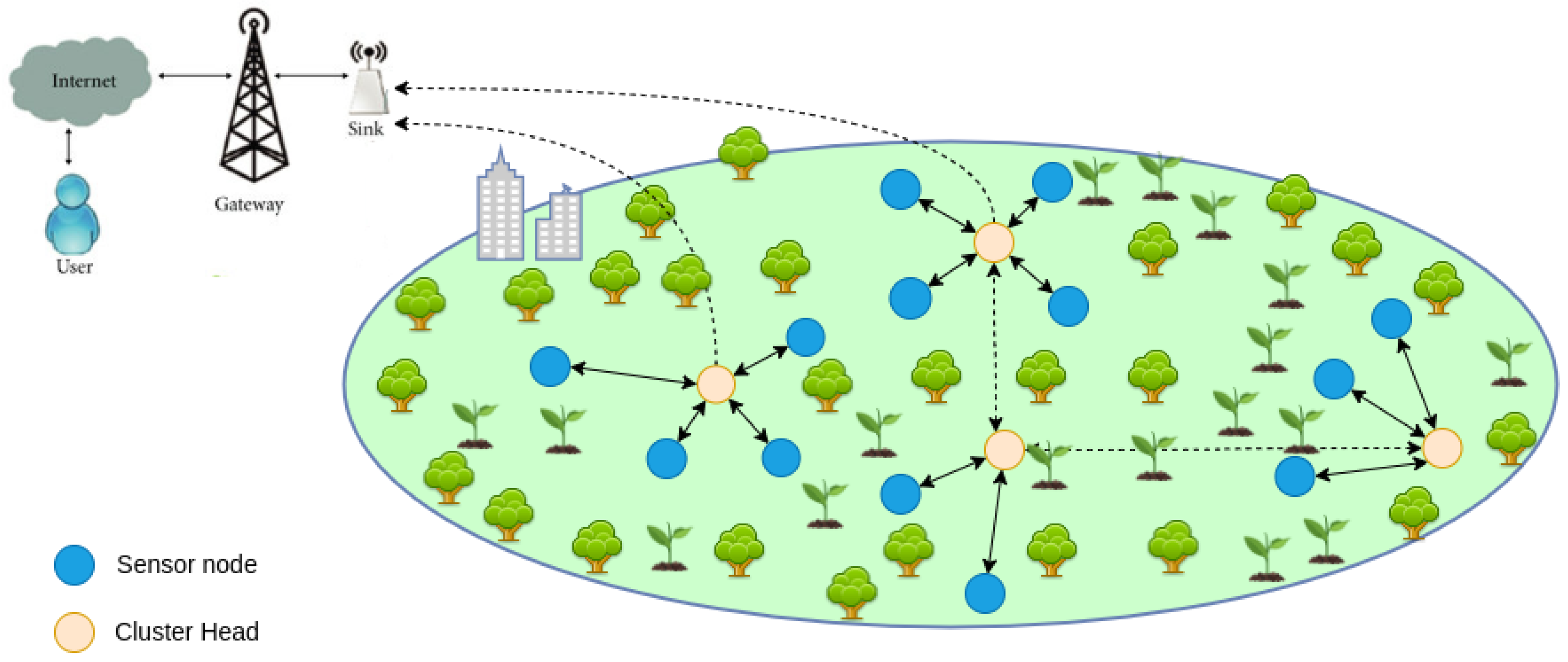
Figure 1 illustrates a hybrid WSN architecture, as discussed in [25,26], serving as the baseline for our study. Multiple sensor nodes are deployed to span a suburban or rural terrain, forming local clusters that cover smaller areas of interest. Cluster heads are selected statically during placement and are equipped with cellular antennas to aggregate and propagate measurements from sensor nodes to a sink node, also placed statically in the vicinity of the network. Communication between nodes is enabled by low-power wireless communication protocols, like ZigBee or 6LoWPAN, whereas cluster heads communicate both with one another and with the sink node using established cellular infrastructure. After receiving sensor node measurements, the sink node acts as a gateway and propagates those measurements to a cloud-based server for storage and data analysis.
We focus our study on transmission frequencies around 1800 MHz, which are used in LTE band 3 [27] and 5G New Radio (NR) n3 [28] frequency bands. In IoT deployments [29] and in Agriculture 4.0 applications [30], 5G has been gaining traction over recent years, further highlighting the significance and applicability of our results.
As area coverage is ensured by placing an adequate number of sensor nodes in the area of interest, network connectivity is not guaranteed, due to variations in terrain conditions that affect link quality. For the purpose of routing incoming traffic to ensure its reliable arrival, accurate PL estimation is required in the placement phase to determine the optimal positioning of cluster heads and the sink node. Optimal placement is achieved by minimizing the path attenuation of the link between cluster heads and the sink node. The quality of this PL estimation determines whether measurement data will reach the cloud-based server and, as a consequence, the Quality of Service (QoS) for the entire network [31].
Various theoretical or empirical models have been devised for estimating PL [32], each with its own assumptions and limitations. Instead of relying on conventional theoretical or empirical mathematical models for PL estimation, we employ CNN models as PL estimators. ANN can potentially capture complex, nonlinear relationships between features employed in PL estimation. In contrast to a fully connected ANN, which can learn the weight of each feature separately, CNN can target specific combinations of features at a time [33] and, in turn, capture the correlation of combined features with respect to PL. This can therefore provide more accurate estimations than conventional theoretical or empirical models.
By providing better PL estimation with the use of ML and specifically using CNN models, our goal is to aid in the development of network topologies with better sensor node link quality, thus enhancing the achieved IoT network connectivity.

3.2. Data Format and Utilization

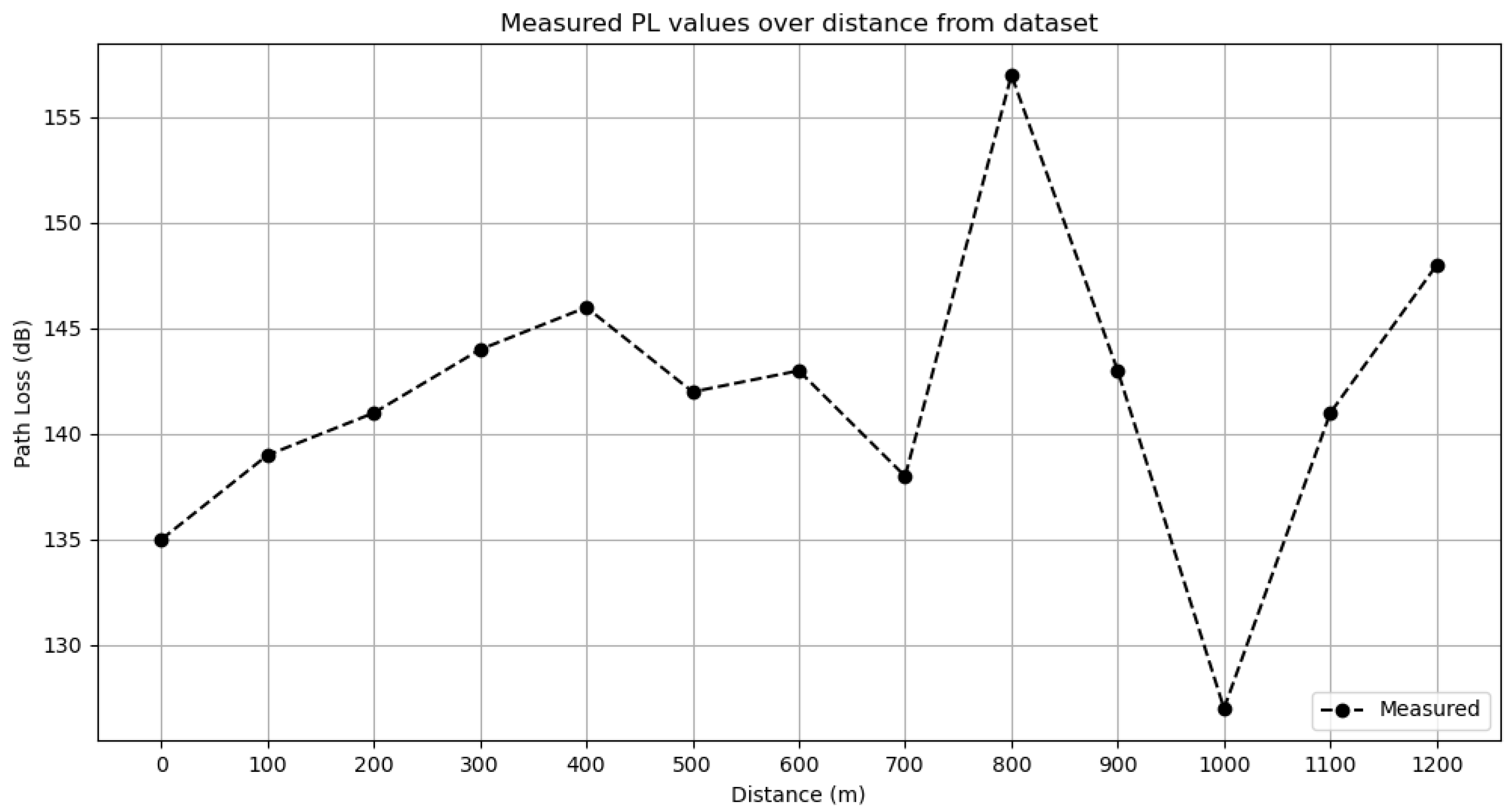
In this study, the dataset provided by [34] was employed. Comprehensive drive test measurements were conducted along three distinct routes (designated as X, Y, and Z) within the premises of Covenant University, located in Ota, Ogun State, Nigeria (Latitude: 6°40′30.3″ N; Longitude: 3°09′46.3″ E). The primary objective was to capture PL data as the mobile receiver traversed away from each of the three base station transmitters operating at a frequency of 1800 MHz. The data acquisition utilized an experimental configuration comprising a Test Mobile Station (TEMS) utilizing a Sony Ericsson W995 handset, along with the Ericsson TEMS Investigation software (version 9.0), a Garmin Global Positioning System (GPS) receiver, and a Windows-based Personal Computer (PC). To ensure reliability, the tests were conducted under favorable climatic conditions and 3 accessible survey routes, X, Y, and Z, while maintaining a controlled vehicle speed of 40 km/h to minimize Doppler effects. The dataset includes 3617 measurements for features such as PL (dB), distance (meters), geographic location (longitude, latitude), elevation (meters), clutter height (meters), and terrain type—each contributing to the modeling of radio signal behavior. These features were captured using integrated GPS data, Digital Terrain Maps (DTMs), and visual inspections. The proposed system model aligns well with the aforementioned dataset in terms of both the operational frequency band used and the terrain type. Statistics on the data are presented in [34] for each route explored separately. Table 1 contains the first-order statistics for measurements in the smart campus dataset across all survey routes explored. A plot of the PL measured values used with respect to distance is presented in Figure 2.

3.3. Data Preprocessing and Reshaping

This study uses a dataset relevant to radio wave PL, characterized by features such as distance from a base station antenna, elevation from the ground, altitude, clutter height, frequency of signal transmitted, and terrain type. Initially, the dataset is split into independent variables (input features) and the dependent variable (ground truth). The input features encompass distance, elevation, altitude, clutter height, frequency, and terrain, while the ground truth is the PL measured value.
Subsequently, the dataset is partitioned into training and testing sets using a standard 80–20 split, ensuring the model’s performance can be assessed on unseen data. The testing dataset is comprised of data instances that are not included in the training dataset.
CNNs have been used extensively in tasks that involve grid-like multi-dimensional data, due to their ability to efficiently capture spatial hierarchies and local patterns. However, PL estimation is mostly concerned with scalar features. In order to employ CNN for PL modeling, a transformation of tabular data into a structure that emulates spatial relationships needs to take place. Multiple CNN models were designed to explore various combinations of features from the dataset. They accept as input one-dimensional rows of different sets of scalar features, with the convolutional kernel focusing on feature pairs at a time.

3.4. CNN Model Architecture, Training and Evaluation

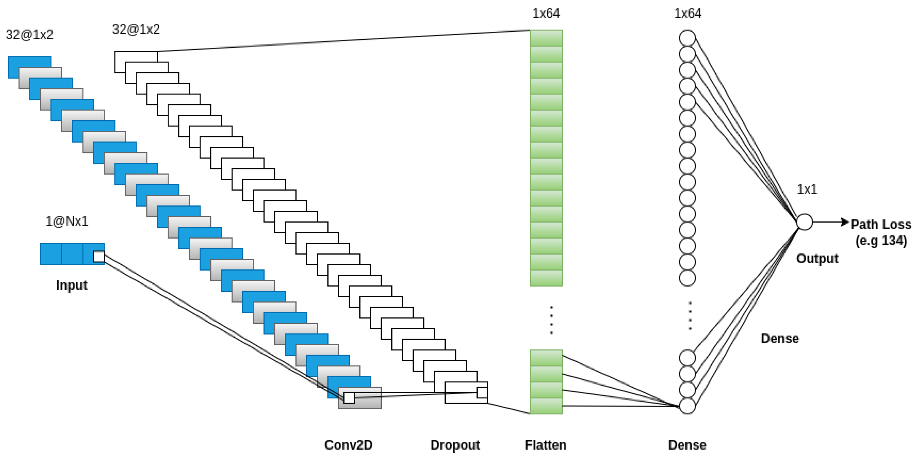
A custom CNN architecture was developed for PL prediction, implemented using Python 3.12.10 and the TensorFlow Keras API. The same architecture was used for all proposed CNN models. The architecture is composed of the following layers:
  • Input Layer: Each input sample is reshaped into a single-row image with N columns of scalar feature measurements and 1 channel. N in this context refers to the number of features used for each of the CNN models. Each feature value corresponds to a single pixel in the single-row image. Consequently, each input data point has input shape (1, N, 1).
  • Conv2D Layer: The first 2D convolution layer employs 32 filters of size (1, 2) with ReLU activation. This implies that the convolution layer is 1D.
  • Dropout Layer: A dropout rate of 0.2 is imposed to mitigate overfitting by randomly disabling a portion of neurons during training.
  • Flatten Layer: This layer transforms the output of the convolution layer into a one-dimensional vector suitable for the following fully connected layers.
  • Dense Layer: The dense layer contains 64 neurons with ReLU activation.
  • Output Layer: A scalar value representing the predicted PL.
The convolutional layer employs filters of size (1, 2), which means it examines pairs of neighboring features simultaneously. For instance, it can learn interactions between distance and elevation or between frequency and terrain, which are often interdependent in PL modeling. This design enables the model to learn intricate feature interdependencies that may be missed by traditional models.
Furthermore, by flattening the convolutional outputs and passing them through dense layers, the model integrates these correlations into a global understanding, enabling the modeling of non-linear interactions among feature correlations, rather than the features individually. The overall architecture balances the advantages of CNN—such as local feature learning and parameter efficiency—with the requirement to handle tabular data efficiently.
The model is compiled using the Adam optimizer [35]. Training takes place over 50 epochs with a batch size of 32. The input layer of the base CNN architecture can be extended and adapted depending on the number of terrain features. Figure 3 illustrates the base CNN model architecture along with its typical hyperparameters.
We used the Optuna method for hyperparameter tuning of the aforementioned CNN architecture [36,37]. The Optuna method involves training a neural network model with various hyperparameters (i.e., number of layers, number of neurons, type of activation functions, etc.), searching for the ones that output the best performing model. The Optuna method has the ability to find optimal or close to optimal hyperparameters that lead to the highest possible prediction accuracy. In total, 50 trials of the Optuna method were employed to minimize the hyperparameters of the CNN architecture within predefined search spaces. An objective function was formulated to evaluate the performance of each hyperparameter configuration, with the primary metric being the minimization of validation loss. The optimization process iteratively explored the search space for each hyperparameter to identify the hyperparameter combination that yielded the lowest validation loss, with the optimal configuration detailed in Table 2. This methodology ensures transparency and reproducibility by explicitly delineating the search space parameters and the optimization strategy employed.

3.5. Propagation Models Implementation

To establish a comparative baseline, several well-known radio propagation models were implemented for benchmarking. The selected propagation models are commonly used in rural or suburban terrains and are adapted to the selected frequency band. Parameters used in the propagation model equations are presented in Table 3.
The heights of the base station and mobile antennas are not specified in [34] so we assume a typical cellular network antenna height of 30 m for the base station, thus h b = 30   m , and a height of 1 m for the mobile measuring antenna height inside the car used for measuring PL, thus h m = 1   m .
  • Free Space Path Loss (FSPL): The Free Space Path Loss model is a fundamental propagation model that provides a theoretical baseline for signal attenuation in ideal conditions. It assumes a clear line-of-sight path between the transmitter and receiver, with no obstructions or atmospheric effects. The PL increases with both distance and frequency. The model predicts that the signal strength decreases proportionally to the square of the distance (inverse-square law) and the square of the frequency. While simple, FSPL is often used as a starting point for more complex propagation models and for understanding the fundamental limitations of radio communication. It provides a theoretical minimum PL; any real-world scenario will experience higher PL due to various environmental factors [38]. The model’s equation expresses PL as follows:
    P L ( d , f ) = 20 l o g 10 ( d / 1000 ) + 20 l o g 10 ( f ) 27.55
  • Okumura–Hata: The Okumura–Hata model, also known as the Hata model, is a popular empirical method for predicting radio wave propagation loss in various environments, including urban, suburban, and open areas. It accounts for signal degradation due to diffraction, reflection, and scattering caused by buildings and other structures. This model, derived from Okumura’s field measurements in Tokyo [39] and mathematically formulated by Hata [40], estimates PL using four key parameters: carrier frequency, distance between transmitter and receiver, base station antenna height, and mobile antenna height. The following model’s equation for suburban environments is used to estimate the expected PL:
    P L ( d , f ) = P L U ( d , f ) 2 ( l o g 10 ( f 28 ) ) 2 5.4
    where P L U ( d , f ) corresponds to the model’s equation for urban environments presented below.
    P L U ( d , f ) = 69.55 + 26.16 l o g 10 ( f ) 13.82 l o g 10 ( h b )
    + ( 44.9 6.55 l o g 10 ( h b ) ) l o g 10 ( d / 1000 ) C H
    The correction factor C H used corresponds to the model’s correction factor for small to medium sized cities.
    C H = 0.8 + ( 1.1 l o g 10 ( f ) 0.7 ) h m 1.56 l o g 10 ( f )
  • COST 231: The COST 231 (Hata) model is a widely adopted empirical radio propagation model developed primarily for predicting signal coverage across diverse European terrains. Often referred to as the Hata model PCS extension, it represents an enhancement of the original Hata model. Distinguished by its broader frequency applicability and structural simplicity, the COST 231 Hata model incorporates correction factors that support its effective deployment across urban, suburban, and rural environments. It supports frequency ranges from 500 MHz to 2000 MHz, transmitter antenna heights between 30 m and 100 m, mobile station heights from 1 m to 10 m, and transmission distances of up to 20 km [41]. The model expresses PL through the following mathematical formulation:
    P L ( d , f ) = 46.3 + 33.9 l o g 10 ( f ) 13.82 l o g 10 ( h b )
    a ( h m , f ) + ( 44.9 6.55 l o g 10 ( h b ) ) l o g 10 ( d / 1000 )
    where a ( h m , f ) corresponds to the following correction factor for transmission node antenna height for suburban or rural environments:
    a ( h m , f ) = ( 1.1 l o g 10 ( f ) 0.7 ) h m ( 1.56 l o g 10 ( f ) 0.8 )
  • Log-Distance Path Loss: The Log-Distance or Log-Normal Path Loss model is a foundational large-scale propagation model that characterizes average signal attenuation as a function of distance between a transmitter and receiver. The model expresses the mean PL as a logarithmic function of the separation distance. In this model, the PL is considered to be a random variable that can be modeled with a log-normal distribution [42]. In the following equation, X σ represents a zero-mean random variable following a log-normal distribution, while the close-in reference distance P L ( d 0 ) is calculated with d 0 = 1   m , assuming a typical macrocell scenario, derived from the FSPL model. The Path Loss exponent γ is set to 3, reflecting typical values in urban cellular networks [43].
    P L ( d ) = P L ( d 0 ) + 10 γ l o g 10 ( d d 0 1000 ) + X σ

4. Results

4.1. Model Performance Metrics

In order to evaluate the performance of our Convolutional Neural Network models, we employed the following key metrics: Mean Squared Error (MSE), Mean Absolute Error (MAE), and Root Mean Squared Error (RMSE). These metrics deliver insights into the model’s accuracy in predicting PL based on previously unseen data.
MSE (Mean Squared Error) measures the average of the squares of the differences between each predicted value from the CNN models and the actual measured values, or ground truth. This metric gives an idea of how close the predictions are to the actual values, with more emphasis on larger errors. The MSE is calculated as follows:
M S E = 1 n i = 1 n ( y i y ^ i ) 2
where
  • n = represents the total number of measured PL values or data points.
  • y i = represents the measured PL value for the i-th data point.
  • y ^ i = represents the predicted PL value for the i-th data point.
MAE (Mean Absolute Error) measures the average of the absolute differences between each predicted value and the corresponding measured value. This metric gives a linear score without amplifying the larger errors as much as MSE. The MAE is calculated as follows:
M A E = 1 n i = 1 n | y i y ^ i |
where
  • n = represents total number of measured PL values or data points.
  • y i = represents the measured PL value for the i-th data point.
  • y ^ i = represents the predicted PL value for the i-th data point.
RMSE (Root Mean Squared Error) measures the average magnitude of the differences between predicted and measured values. This metric can express error in terms of the original measurement units, as it represents the square root of the MSE. It also reflects the variability of the prediction errors. The RMSE is calculated as follows:
R M S E = 1 n i = 1 n ( y i y ^ i ) 2
where
  • n = represents the total number of measured PL values or data points.
  • y i = represents the measured PL value for the i-th data point.
  • y ^ i = represents the predicted PL value, for the i-th data point.
In the context of regression, a model that offers good predictive capabilities should have MSE, MAE, and RMSE metric values as low as possible, as these metrics reflect better alignment with the ground truth data.

4.2. CNN Models Performance Analysis

To explore the influence of each of the features provided by the dataset on the resulting PL predictions, we experimented with multiple CNN models that use different combinations of features. All CNN models include the distance between the transmitting and receiving antennas as a mandatory input feature. The error metrics derived by the evaluation of each model are presented in Table 4.
The evaluation of various CNN models highlights the influence of different input features on PL prediction accuracy. The baseline model, CNN d, which relies solely on distance as input, yields an RMSE of 10.86, establishing a reference for comparison. It is expected that this model exhibits poorer performance than the following ones, as its training relies on a reduced feature set with limited correlation to PL. Therefore, its ability to model PL is limited.
Enhancing this model with elevation data (CNN d-e) leads to a substantial improvement, achieving the lowest RMSE of 7.84, indicating that elevation is a highly informative feature to improve model accuracy. In contrast, the addition of clutter height to distance and elevation (CNN d-e-c) results in a modest increase in error (RMSE 9.43), suggesting that while clutter may contribute to specific contexts, it does not improve accuracy beyond the benefit already provided by elevation. The CNN d-c model, using distance and clutter height, performs similarly (RMSE 9.34).
Models incorporating altitude show less favorable results. The CNN d-a model, combining distance and altitude, yields a higher RMSE of 11.40, implying a limited value in altitude alone. The combined use of elevation and altitude in CNN d-e-a leads to the poorest performance (RMSE 16.53), likely due to feature redundancy, as both of those features convey similar information. Elevation denotes the height above ground level, while altitude refers to height above sea level. As the distance from the ground increases, the distance from sea level is expected to increase too. This redundancy can confuse the CNN during training, leading to poorer generalization and higher prediction errors. Moreover, altitude measurements can have higher uncertainty or noise compared to other features, especially in a real-world, suburban setting. Incorporating noisy features can degrade model performance, as the CNN may overfit to irrelevant fluctuations rather than underlying patterns.
However, supplementing this combination with clutter height (CNN d-e-a-c) improves performance (RMSE 9.97), suggesting that clutter height information may help the training process by minimizing the effect of redundancy or noise from altitude and elevation. Similarly, the CNN d-a-c model (RMSE 9.87) shows that even without elevation, a carefully chosen mix of features can yield competitive performance.
In general, the analysis underscores the dominant role of elevation data in improving CNN-based PL prediction, while also revealing complex feature interactions that must be carefully balanced to achieve optimal accuracy.
We conclude that the best CNN model for PL prediction is CNN d-e. This model achieves the lowest MSE, MAE, and RMSE metrics among all the CNN models listed. This implies that even features that are considered fundamental in the field of PL prediction, such as distance and elevation, offer sufficient information for accurate PL predictions across links in rural and suburban terrains. The inclusion of more features degrades the performance of our models, implying that the additional features fail to contribute further relevant information for PL estimation.
Figure 4 provides a bar plot of the RMSE metrics for each CNN model trained. All CNN models exhibit relatively low error rates within the range (7.5 dB, 12.5 dB). It can be observed clearly that CNN d-e outperforms its counterparts in terms of RMSE.
In Figure 5, a line plot illustrates the measured PL values from the dataset and the predicted PL values from the various CNN models employed with respect to distance. As anticipated, the CNN d-e model exhibits a better fit to the measured data than the propagation models, aligning with its observed lower error rates. Noticeable discrepancies appear between predicted and measured PL values at 800 m and 1000 m, coinciding with deviations from the general PL trend within the dataset. PL tends to increase with the square of the distance, and the deviations in the measured PL values at 800 m and 1000 m can be attributed to errors in the data collection process and variations in the terrain, such as potential obstacles between the measurement and base station antennas. Moreover, only survey route Z explores distances beyond 883 m, and therefore, the model has limited exposure to the characteristics of PL at these distances and, consequently, its ability to learn is also limited. While CNN models can adapt to some extent to those discrepancies, fitting those observations more accurately would imply overfitting.

4.3. Propagation Models Performance Comparison

In order to further evaluate the performance of our CNN model, we compare the best of our proposed CNN models, notably CNN d-e, with the propagation models discussed above. The findings of this comparative evaluation clearly illustrate that the CNN model achieves the lowest MSE and MAE errors among all well-known models and thus surpasses conventional approaches in accurately predicting PL, thereby validating the application of deep learning methodologies in this domain. Table 5 demonstrates the error metrics for all propagation models’ predictions with respect to the measured PL values from the dataset.
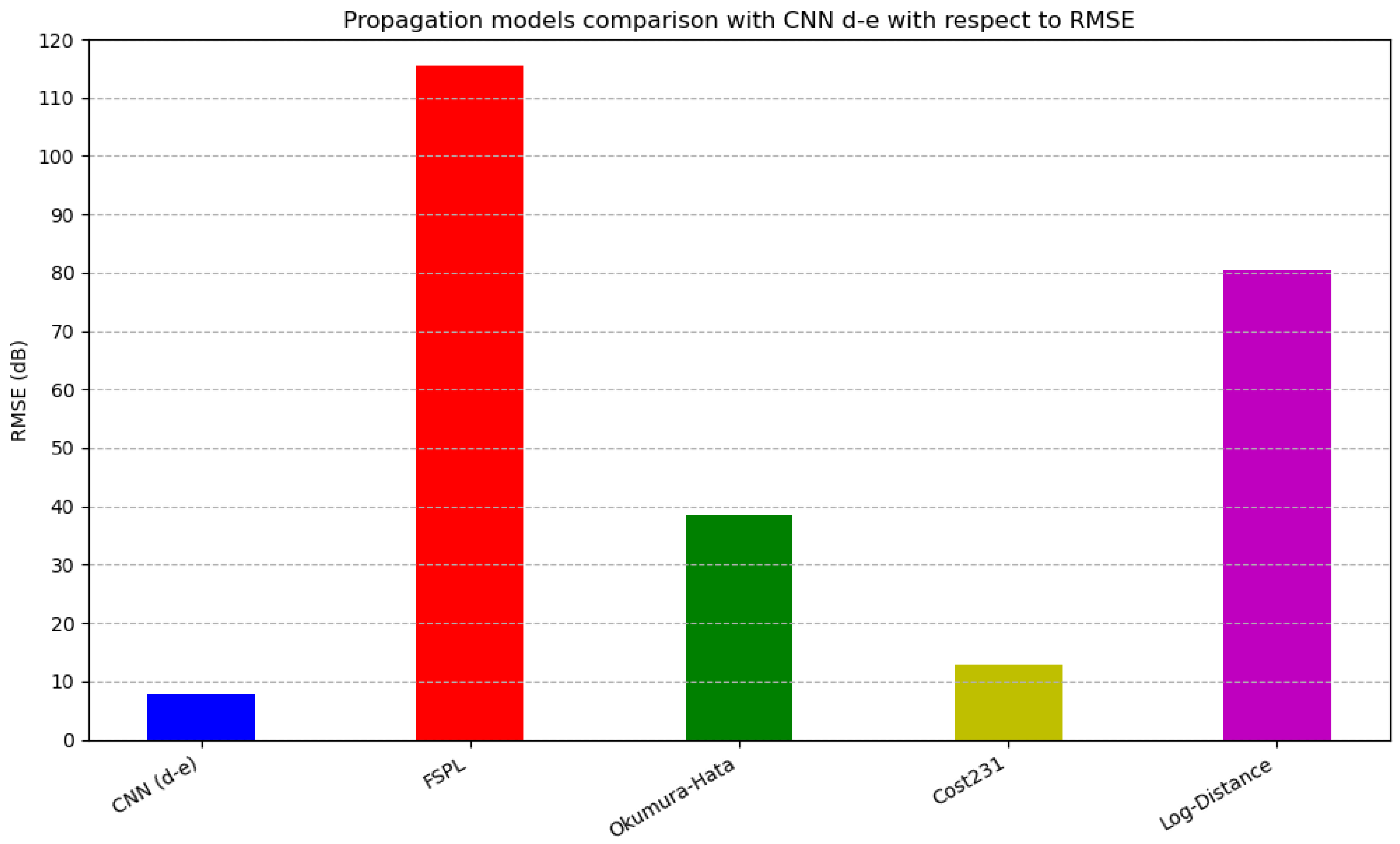
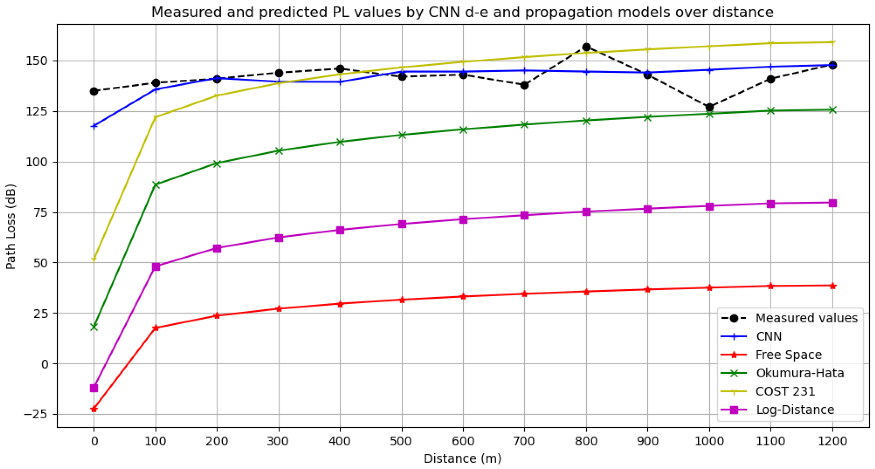
Figure 6 depicts the RMSE metrics of the CNN d-e model and the benchmark propagation models. All propagation models demonstrated higher RMSE values than CNN d-e, as well as other CNN models, rendering CNN d-e the best PL predictor. The higher error rates of commonly used propagation models, compared to the CNN model’s performance, imply that, while real-world applications achieve good enough QoS using those propagation models, the use of CNN in such applications could provide substantial improvements in QoS by allowing greater liberty in cluster head placement.
Figure 7 illustrates the measured PL values alongside the predictions from the best performing CNN d-e model and the propagation models discussed over distance. The CNN model exhibits excellent adaptability, with predictions closely aligned with the measured values. The FSPL and Log-Distance models struggled to accurately predict the measured PL values and showed strong deviation from them. This can be attributed to the assumptions of free space and line-of-sight visibility used in those models, which do not hold in the suburban terrain where measurements were made. FSPL serves as a reference for the minimum expected PL values with respect to distance, while the poor performance of Log-Distance implies the existence of obstacles and interference in a suburban terrain. The Okumura–Hata model demonstrated lower accuracy compared to the CNN model, primarily because its design is optimized for frequencies up to 1500 MHz, resulting in underestimated PL values at higher frequencies. Although the COST 231 model exhibited commendable performance, the CNN d-e model proved superior in terms of the error metrics. These results are consistent with the lower MSE, MAE, and RMSE values observed across all benchmark propagation models.
A more detailed presentation of the performance comparison between CNN d-e and the propagation models is presented in Table 6. The Absolute Percentage Error (APE) of the predicted PL values from either the CNN d-e or the traditional propagation models, relative to the measured values, is presented per 100 m of distance. We use APE to quantify the deviation, in percentage, of each predicted PL value, at 100 m intervals, from the measured PL values. APE is calculated using the following equation:
A P E = | y i y ^ i | | y ^ i | 100%
where
  • y i = represents the measured PL value for the i-th data point.
  • y ^ i = represents the predicted PL value for the i-th data point.
Table 6 thoroughly verifies that CNN d-e has the lowest percentage deviation from the measured PL data per 100 m distance from all conventional propagation models. In some instances, a propagation model might exhibit a lower deviation from the corresponding measured PL values; however, the CNN model consistently maintains low deviation across all distances. The CNN model might be able to achieve even lower deviations and error rates by augmenting the training dataset with more diverse PL measurements, an advantage not offered by conventional PL propagation models.
Table 6. Performance comparison of CNN d-e and propagation models per 100 m of distance.
DistanceCNN d-eFSPLOkumura–HataCOST 231Log-Distance
0 m1.97%116.62%86.61%61.85%107.97%
100 m2.17%87.37%36.31%12.27%64.57%
200 m0.52%83.25%29.64%5.94%58.62%
300 m2.39%81.18%26.85%3.64%55.86%
400 m4.50%79.73%24.84%1.95%53.90%
500 m3.61%77.78%20.29%3.24%50.54%
600 m3.37%76.84%18.92%4.44%49.24%
700 m4.06%75.04%14.29%9.92%45.96%
800 m6.69%77.31%23.34%2.05%51.37%
900 m5.65%74.40%14.62%8.74%45.57%
1000 m20.73%70.47%2.63%23.68%37.66%
1100 m9.85%72.79%11.22%12.48%42.93%
1200 m5.26%73.90%15.10%7.48%45.37%

5. Conclusions and Future Work

This study clearly demonstrates the effectiveness of the proposed customized CNN model in predicting PL within WSN deployed in a smart campus environment. Various CNN models were constructed to learn from different combinations of features, and the best performing CNN, d-e, proved to consistently outperform conventional propagation models, including FSPL, Okumura–Hata, COST 231, and Log-Distance, by more accurately capturing the complex signal propagation behaviors. This superior performance can be attributed to the model’s architecture, which is optimized to learn the intricate correlations between terrain features, such as distance between antennas, elevation from ground, altitude, and clutter height. As a result, the CNN model significantly enhances PL prediction accuracy, leading to improved node connectivity and overall network performance—critical factors for ensuring reliable communication in IoT and WSN applications.
The superior performance of the CNN d-e model suggests that distance and elevation from the ground are the most salient features for accurate PL estimation in this context. While terrain type and frequency of transmitted signals are also recognized as critical factors influencing PL, their impact could not be further investigated in this study due to the static nature of these features within the available dataset. This research indicates that distance and elevation are highly effective for PL prediction, underscoring the importance of collecting accurate and diverse measurements for these parameters in future data acquisition efforts to facilitate enhanced model training.
Building on the success of the CNN model in the smart campus context, future research will focus on extending its applicability to a broader range of environments. Key directions include the use of transfer learning techniques to adapt pre-trained models for new contexts with limited data and the development of hybrid approaches that integrate CNN with traditional propagation models for greater accuracy in complex settings. By selecting suitable input features, the proposed model can be trained and applied to any operating frequency and terrain type. To extend its applicability to other environments, additional datasets and environment-specific training would be necessary. Expanding the training dataset to include variations in geography, terrain, building structures, foliage density, frequency bands, and weather conditions will further enhance the model’s generalization capabilities.
Future research will also undertake a comprehensive comparative analysis to evaluate the performance of the CNN PL prediction models presented in this paper against a diverse range of alternative ML techniques. This comparative investigation aims to establish a robust understanding of the CNN model’s relative strengths and weaknesses, identify areas for potential improvement, and determine the most suitable ML approach for PL prediction under varying environmental conditions and data availability constraints. Moreover, incorporating advanced deep learning techniques—such as Recurrent Neural Networks (RNNs) for temporal modeling or Graph Neural Networks (GNNs) for capturing spatial relationships—may further enhance prediction performance. Collectively, these advancements aim to establish a versatile and robust PL prediction framework, capable of supporting efficient, reliable, and energy-aware WSN deployments across a wide range of real-world deployment scenarios.

Author Contributions

Conceptualization, G.P., A.X., C.C., D.K. and M.P.P.; methodology, G.P., A.X., C.C., D.K. and M.P.P.; software, G.P. and M.P.P.; validation, G.P. and M.P.P.; formal analysis, G.P. and M.P.P.; investigation, G.P., A.X. and M.P.P.; resources, G.P.; data curation, G.P. and M.P.P.; writing—original draft preparation, G.P., A.X. and M.P.P.; writing—review and editing, A.X., C.C. and D.K.; visualization, G.P. and M.P.P.; supervision, A.X., C.C. and D.K. All authors have read and agreed to the published version of the manuscript.

Funding

This research received no external funding.

Data Availability Statement

The dataset used is provided by the authors of [34] as supplementary material.

Conflicts of Interest

The authors declare no conflicts of interest.

Abbreviations

The following abbreviations are used in this manuscript:
IoTInternet of Things
WSNWireless Sensor Network
PLPath Loss
CNNConvolutional Neural Network
ANNArtificial Neural Network
QoSQuality of Service
MSEMean Square Error
RMSERoot Mean Square Error
MAEMean Absolute Error
APEAverage Percentage Error
FSPLFree Space Path Loss

References

  1. Heller, A. The Sensing Internet—A Discussion on Its Impact on Rural Areas. Future Internet 2015, 7, 363–371. [Google Scholar] [CrossRef]
  2. Farhan, L.; Kharel, R.; Kaiwartya, O.; Quiroz-Castellanos, M.; Alissa, A.; Abdulsalam, M. A concise review on internet of things (IoT)—Problems, challenges and opportunities. In Proceedings of the 11th International Symposium on Communication Systems, Networks & Digital Signal Processing (CSNDSP), Budapest, Hungary, 18–20 July 2018; pp. 1–6. [Google Scholar] [CrossRef]
  3. Idigo, V.E. Wireless Sensor Networks for Environmental Monitoring: A Review. Int. J. Eng. Trends Technol.—IJETT 2020, 68, 68–71. Available online: https://ijettjournal.org/archive/ijett-v68i1p210 (accessed on 30 July 2025).
  4. Popoola, S.I.; Adetiba, E.; Atayero, A.A.; Calafate, C.T. Artificial Neural Network-Based Path Loss Prediction Model for Rural Propagation Environments. ResearchGate. Available online: https://www.researchgate.net/publication/317844806_Artificial_Neural_Network-Based_Path_Loss_Prediction_Model_for_Rural_Propagation_Environments (accessed on 30 July 2025).
  5. Kopawar, N.A.; Wankhede, K.G. Internet of Things in Agriculture: A Review. Int. J. Sci. Res. Sci. Eng. Technol. 2024, 11, 161–165. [Google Scholar] [CrossRef]
  6. Chebil, J.; Lwas, A.K.; Islam, M.R.; Zyoud, A.-H. Comparison of Empirical Propagation Path Loss Models for Mobile Communications in the Suburban Area of Kuala Lumpur. In Proceedings of the 2011 4th International Conference on Mechatronics (ICOM), Kuala Lumpur, Malaysia, 17–19 May 2011. [Google Scholar] [CrossRef]
  7. Kochhar, A.; Kaur, P.; Singh, P.; Sharma, S. Protocols for Wireless Sensor Networks: A Survey. J. Telecommun. Inf. Technol. 2018, 1, 77–87. [Google Scholar] [CrossRef]
  8. Galvan-Tejada, G.M.; Aguilar-Torrentera, J. Analysis of Propagation for Wireless Sensor Networks in Outdoors. Prog. Electromagn. Res. B 2019, 83, 153–175. [Google Scholar] [CrossRef]
  9. Jabbar, D.J.; Al-Nakkash, A.H. Field Measurement and Empirical Models for Radio Signal Propagation Prediction in Baghdad. In Proceedings of the 2019 4th Scientific International Conference Najaf (SICN), Al-Najef, Iraq, 29–30 April 2019; pp. 31–36. [Google Scholar] [CrossRef]
  10. Barrios-Ulloa, A.; Ariza-Colpas, P.; Sánchez-Moreno, H.; Quintero-Linero, A.; De la Hoz-Franco, E. Modeling Radio Wave Propagation for Wireless Sensor Networks in Vegetated Environments: A Systematic Literature Review. Sensors 2022, 22, 5285. [Google Scholar] [CrossRef]
  11. Tang, W.; Ma, X.; Wei, J.; Wang, Z. Measurement and Analysis of Near-Ground Propagation Models under Different Terrains for Wireless Sensor Networks. Sensors 2019, 19, 1901. [Google Scholar] [CrossRef]
  12. Obot, E.P.; Onuu, M.U.; Arikpo, J.U.; Nwosu, C.N. A Comparative Study of Path Loss Models in the Ultra-High Frequency Band in a Vegetated Environment; Research Square: Durham, NC, USA, 2022. [Google Scholar] [CrossRef]
  13. Sharma, P.K.; Singh, R.K. Comparative Analysis of Propagation Path Loss Models with Field Measured Data. Int. J. Eng. Sci. Technol. 2010, 2, 2008–2013. Available online: https://www.researchgate.net/publication/50281818_Comparative_Analysis_of_Propagation_Path_loss_Models_with_Field_Measured_Data (accessed on 30 July 2025).
  14. Ojo, S.; Sari, A.; Ojo, T.P. Path loss modeling: A machine learning based approach using support vector regression and radial basis function models. Open J. Appl. Sci. 2022, 12, 990–1010. [Google Scholar] [CrossRef]
  15. Zhang, Y.; Wen, J.; Yang, G.; He, Z.; Wang, J. Path loss prediction based on machine learning: Principle, method, and data expansion. Appl. Sci. 2019, 9, 1908. [Google Scholar] [CrossRef]
  16. Iliev, I.; Velchev, Y.; Petkov, P.Z.; Bonev, B.; Iliev, G.; Nachev, I. A machine learning approach for path loss prediction using combination of regression and classification models. Sensors 2024, 24, 5855. [Google Scholar] [CrossRef]
  17. Moraitis, N.; Tsipi, L.; Vouyioukas, D.; Gkioni, A.; Louvros, S. Performance Evaluation of Machine Learning Methods for Path Loss Prediction in Rural Environment at 3.7 GHz. Wirel. Netw. 2021, 27, 4169–4188. [Google Scholar] [CrossRef]
  18. Jo, H.-S.; Park, C.; Lee, E.; Choi, H.K.; Park, J. Path Loss Prediction Based on Machine Learning Techniques: Principal Component Analysis, Artificial Neural Network, and Gaussian Process. Sensors 2020, 20, 1927. [Google Scholar] [CrossRef] [PubMed]
  19. Idogho, J.; George, G. Path Loss Prediction Based on Machine Learning Techniques: Support Vector Machine, Artificial Neural Network, and Multilinear Regression Model. Open J. Phys. Sci. 2022, 3, 1–22. [Google Scholar] [CrossRef]
  20. Popoola, S.I.; Adetiba, E.; Atayero, A.A.; Faruk, N.; Calafate, C.T. Optimal Model for Path Loss Predictions Using Feed-Forward Neural Networks. Cogent Eng. 2018, 5, 1444345. [Google Scholar] [CrossRef]
  21. Kwon, B.; Son, H. Accurate Path Loss Prediction Using a Neural Network Ensemble Method. Sensors 2024, 24, 304. [Google Scholar] [CrossRef]
  22. Qiu, Z.; He, R.; Yang, M.; Zhou, S.; Yu, L.; Wang, C.; Zhang, Y.; Fan, J.; Ai, B. CNN-Based Path Loss Prediction with Enhanced Satellite Images. IEEE Antennas Wirel. Propag. Lett. 2023, 23, 189–193. [Google Scholar] [CrossRef]
  23. Thrane, J.; Zibar, D.; Christiansen, H.L. Model-Aided Deep Learning Method for Path Loss Prediction in Mobile Communication Systems at 2.6 GHz. IEEE Access 2016, 8, 7925–7936. [Google Scholar] [CrossRef]
  24. Hehn, T.M.; Orekondy, T.; Shental, O.; Behboodi, A.; Bucheli, J.; Doshi, A.; Namgoong, J.; Yoo, T.; Sampath, A.; Soriaga, J.B. Transformer-Based Neural Surrogate for Link-Level Path Loss Prediction from Variable-Sized Maps. In Proceedings of the GLOBECOM 2023—2023 IEEE Global Communications Conference, Kuala Lumpur, Malaysia, 4–8 December 2023; pp. 4804–4809. [Google Scholar] [CrossRef]
  25. Liang, Q.; Durrani, T.S.; Pi, Y.; Samn, S.W. Hybrid Wireless Sensor Networks: Theory and Design. Int. J. Distrib. Sens. Netw. 2016, 12, 8253168. [Google Scholar] [CrossRef]
  26. Porter, J.H.; Lin, C.C. Hybrid Networks and Ecological Sensing. Smart Sens. Meas. Instrum. 2013, 99–124. [Google Scholar] [CrossRef]
  27. Evolved Universal Terrestrial Radio Access (E-UTRA); User Equipment (UE) radio transmission and Reception. Available online: https://portal.3gpp.org/desktopmodules/Specifications/SpecificationDetails.aspx?specificationId=2411 (accessed on 30 July 2025).
  28. NR; User Equipment (UE) Radio Transmission and Reception; Part 1: Range 1 Standalone. Available online: https://portal.3gpp.org/desktopmodules/Specifications/SpecificationDetails.aspx?specificationId=3283 (accessed on 30 July 2025).
  29. Agiwal, M.; Roy, A.; Saxena, N. Next Generation 5G Wireless Networks: A Comprehensive Survey. IEEE Commun. Surv. Tutor. 2016, 18, 1617–1655. [Google Scholar] [CrossRef]
  30. Raj, M.; Gupta, S.; Chamola, V.; Elhence, A.; Garg, T.; Atiquzzaman, M.; Niyato, D. A Survey on the Role of Internet of Things for Adopting and Promoting Agriculture 4.0. J. Netw. Comput. Appl. 2021, 187, 103107. [Google Scholar] [CrossRef]
  31. Kurt, S.; Tavli, B. Propagation Model Alternatives for Outdoor Wireless Sensor Networks. In Proceedings of the 2013 IFIP Wireless Days (WD), Valencia, Spain, 13–15 November 2013; pp. 1–3. [Google Scholar] [CrossRef]
  32. Alobaidy, H.A.H.; Jit Singh, M.; Behjati, M.; Nordin, R.; Abdullah, N.F. Wireless Transmissions, Propagation and Channel Modelling for IoT Technologies: Applications and Challenges. IEEE Access 2022, 10, 24095–24131. [Google Scholar] [CrossRef]
  33. Li, Z.; Liu, F.; Yang, W.; Peng, S.; Zhou, J. A survey of convolutional neural networks: Analysis, applications, and prospects. IEEE Trans. Neural Netw. Learn. Syst. 2022, 33, 6999–7019. [Google Scholar] [CrossRef]
  34. Popoola, S.I.; Atayero, A.A.; Arausi, O.D.; Matthews, V.O. Path Loss Dataset for Modeling Radio Wave Propagation in Smart Campus Environment. Data Brief 2018, 17, 1062–1073. [Google Scholar] [CrossRef] [PubMed]
  35. Kingma, D.P.; Ba, J. Adam: A Method for Stochastic Optimization. arXiv 2014, arXiv:1412.6980. [Google Scholar] [CrossRef]
  36. Elmezughi, M.K.; Salih, O.; Afullo, T.J.; Duffy, K.J. Path Loss Modeling Based on Neural Networks and Ensemble Method for Future Wireless Networks. Heliyon 2023, 9, e19685. [Google Scholar] [CrossRef] [PubMed]
  37. Akiba, T.; Sano, S.; Yanase, T.; Ohta, T.; Koyama, M. Optuna: A Next-Generation Hyperparameter Optimization Framework. In Proceedings of the 25th ACM SIGKDD International Conference on Knowledge Discovery & Data Mining, Anchorage, AK, USA, 4–8 August 2019. [Google Scholar] [CrossRef]
  38. Friis, H.T. A Note on a Simple Transmission Formula. Proc. IRE 1946, 34, 254–256. [Google Scholar] [CrossRef]
  39. Okumura, Y.; Ohmori, E.; Kawano, T.; Fukuda, K. Field strength and its variability in VHF and UHF land-mobile radio service. Rev. Electr. Commun. Lab. 1968, 16, 825–873. (In Japanese) [Google Scholar]
  40. Hata, M. Empirical Formula for Propagation Loss in Land Mobile Radio Services. IEEE Trans. Veh. Technol. 1980, 29, 317–325. [Google Scholar] [CrossRef]
  41. Final Report for COST Action 231. Available online: https://www.lx.it.pt/cost231/final_report.htm (accessed on 7 July 2025).
  42. Log Distance Path Loss or Log Normal Shadowing Model. Available online: https://www.gaussianwaves.com/2013/09/log-distance-path-loss-or-log-normal-shadowing-model/ (accessed on 7 July 2025).
  43. Srinivasa, S.; Haenggi, M. Path loss exponent estimation in a large field of interferers. arXiv 2008, arXiv:0802.0351. [Google Scholar] [CrossRef]
Figure 1. Reference hybrid Wireless Sensor Network architecture.
Iot 06 00041 g001
Figure 2. Dataset PL measurements with respect to distance.
Iot 06 00041 g002
Figure 3. CNN model architecture.
Iot 06 00041 g003
Figure 4. CNN models comparison with respect to RMSE.
Iot 06 00041 g004
Figure 5. Measured and predicted PL values by the CNN models over distance.
Iot 06 00041 g005
Figure 6. Propagation models comparison with CNN d-e with respect to RMSE.
Iot 06 00041 g006
Figure 7. Measured and predicted PL values by CNN d-e and propagation models over distance.
Iot 06 00041 g007
Table 1. First-order statistics for dataset features over all survey routes.
Elevation (m)Altitude (m)Clutter Height (m)Distance (m)Path Loss (dB)
Mean54.2854.755.78439.53143.08
Median54.0054.006.00376.00145.00
Mode63.0052.006.00138.00147.00
Std. Deviation5.823.882.68269.589.13
Variance33.8315.057.2072,672.0683.33
Kurtosis−1.31−0.529.04−0.721.97
Skewness0.170.663.020.40−1.21
Minimum45.0049.004.001.00104.00
Maximum64.0064.0016.001132.00162.00
Table 2. CNN hyperparameter configuration.
HyperparameterSearch SpaceValue Proposed by Optuna
Conv2D Layer
Filters{16, 32, 64, 128}32
Kernel Size{(1, 2), (1, 3)}(1, 2)
Activation-ReLU
Input Shape-(1, N, 1)
Dropout Layer
Dropout Rate[0.1, 0.5]0.2
Dense Layer
Number of Neurons{32, 64, 128}64
Activation-ReLU
Training Configuration
Optimizer-Adam
Learning Rate[ 1 × 10 5 , 1 × 10 2 ] 1 × 10 3
Loss Function-Mean Square Error
Epochs-50
Batch Size-32
Train—Test Split-80–20%
Table 3. Parameters used in propagation models.
SymbolDescriptionUnits
P L Path LossdB
fOperating frequencyMHz
dDistance between transmit and receive antennasm
h b Base station antenna heightm
h m Transmitting node antenna heightm
Table 4. Performance comparison of CNN models.
CNN ModelInput FeaturesMSEMAERMSE
CNN dDistance117.979.2710.86
CNN d-eDistance, Elevation61.426.087.84
CNN d-e-cDistance, Elevation, Clutter Height88.907.659.428
CNN d-cDistance, Clutter Height87.187.879.337
CNN d-aDistance, Altitude129.989.6911.40
CNN d-e-aDistance, Elevation, Altitude273.5714.8616.53
CNN d-e-a-cDistance, Elevation, Altitude, Clutter Height99.318.509.965
CNN d-a-cDistance, Altitude, Clutter Height97.448.379.871
Table 5. Performance comparison of CNN d-e and propagation models.
ModelMSEMAERMSE
CNN d-e61.426.087.84
FSPL13,316.85115.06115.40
Okumura–Hata1487.8336.4838.57
COST 231166.619.6112.91
Log-Distance6450.5179.5580.32
Disclaimer/Publisher’s Note: The statements, opinions and data contained in all publications are solely those of the individual author(s) and contributor(s) and not of MDPI and/or the editor(s). MDPI and/or the editor(s) disclaim responsibility for any injury to people or property resulting from any ideas, methods, instructions or products referred to in the content.