Abstract
In the derived approach, an analysis is performed on Twitter data for World Cup soccer 2014 held in Brazil to detect the sentiment of the people throughout the world using machine learning techniques. By filtering and analyzing the data using natural language processing techniques, sentiment polarity was calculated based on the emotion words detected in the user tweets. The dataset is normalized to be used by machine learning algorithms and prepared using natural language processing techniques like word tokenization, stemming and lemmatization, part-of-speech (POS) tagger, name entity recognition (NER), and parser to extract emotions for the textual data from each tweet. This approach is implemented using Python programming language and Natural Language Toolkit (NLTK). A derived algorithm extracts emotional words using WordNet with its POS (part-of-speech) for the word in a sentence that has a meaning in the current context, and is assigned sentiment polarity using the SentiWordNet dictionary or using a lexicon-based method. The resultant polarity assigned is further analyzed using naïve Bayes, support vector machine (SVM), K-nearest neighbor (KNN), and random forest machine learning algorithms and visualized on the Weka platform. Naïve Bayes gives the best accuracy of 88.17% whereas random forest gives the best area under the receiver operating characteristics curve (AUC) of 0.97.
1. Introduction
In this advancing world of technology, expressing emotions, feelings, and views regarding any and every situation is much easier through social networking sites. Sentiment analysis along with opinion mining are two processes that aid in classifying and investigating the behavior and approach of customers in regards to the brand, product, events, company, and customer services [1]. Sentiment analysis can be defined as the automatic process of extracting the emotions from the user’s written text by processing unstructured information and preparing a model to extract the knowledge from it [2].
In this paper, one such social networking site is taken into account, which is among the largest networking sites, Twitter. Looking at the statistics, users that are active monthly range around 316 million, and on an average, about 500 million tweets are sent daily [3]. There are many approaches used for sentiment analysis on linguistic data, and the approach to be used depends on the nature of the data and the platform. Most research carried out in the field of sentiment analysis employs lexicon-based analysis or machine learning techniques. Machine learning techniques control the data processing by the use of machine learning algorithms and by classifying the linguistic data by representing them in vector form [4]. On the other side, a lexicon-based (also called dictionary-based) approach classifies the linguistic data using a dictionary lookup database. During this classification, it computes sentence- or document-level sentiment polarity using lexicon databases for processing linguistic data like WordNet, SentiWordNet, and treebanks. Moreover, a lexicon dictionary or database contains the opinionated words that are classified by positive and negative word type, and the description of the word that occurs in the current context. For each word in the document, it is assigned a numeric score; the average score is computed by summing up all the numeric scores and sentiment polarity is assigned to the document. Using this approach, the words in the sentence are considered in the form of vectors and analyzed using different machine learning algorithms like naïve Bayes, support vector machine (SVM), and maximum entropy. The data are trained accordingly, which can be applied to machine learning algorithms.
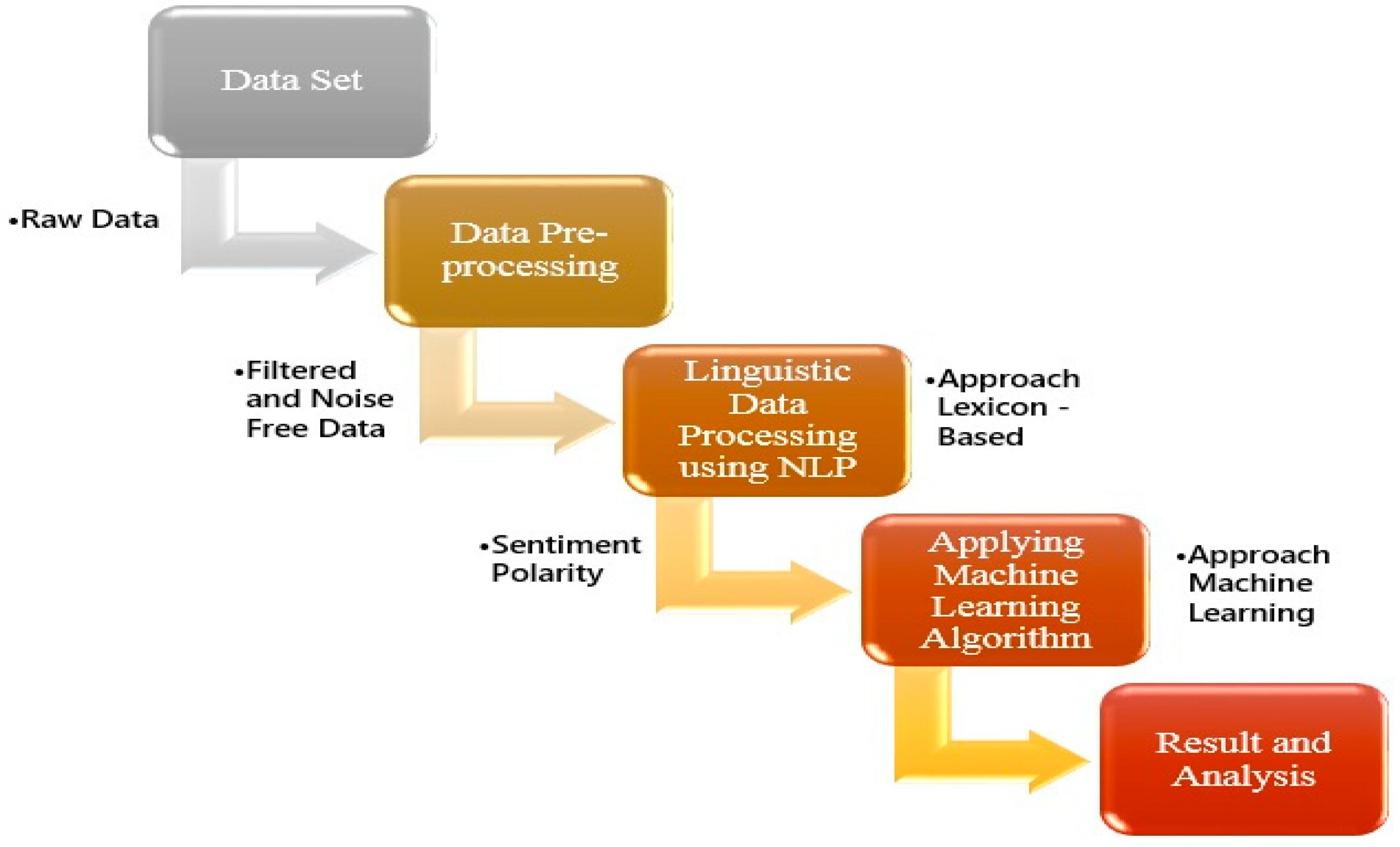
In this paper, both approaches were combined, namely lexicon-based and machine learning for sentiment analysis of Twitter data. These algorithms were implemented for the preprocessing of a dataset, and filtering and reducing the noise from the dataset. In this approach, the core linguistic data processing algorithm using natural language processing (NLP) has been designed and implemented, and sentiment polarity is assigned to the tweets using a lexicon-based approach. Later, the resultant dataset was trained using machine learning algorithms, naïve Bayes, SVM (support vector machine), K-nearest neighbor (KNN), and random forest for measuring the accuracy of the training dataset and comparison of the results was accomplished. An abstract view of the derived approach that combines lexicon-based and machine learning for sentiment analysis is shown in Figure 1.
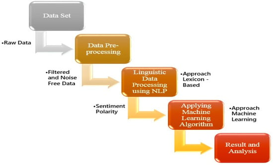
Figure 1.
Overview of approach for sentiment analysis.
2. Related Work
In this era, information sharing through social media has increased and most users actively share their personal ideas and information publicly. This information for an analyst or researcher is a gold mine to dig out the valuable information for strategic decision-making [5]. Fishing out sentiments embodied in the user’s written text, in the world of social media is known as sentiment analysis or opinion mining. Firmino Alves et al. [6] state that from the beginning of the 21st century, sentiment analysis has been one of the most interesting as well as active research topics in the domain of natural language processing. It helps the decision maker to understand the responses of people towards a particular topic and aids in determining whether the event is positive, negative, or neutral. Twitter has been considered a very important platform for data mining by many researchers. Hemalatha et al. [7] discuss that the Twitter platform contains much relevant information on particular events with hashtags that have been followed and accepted by many popular personalities. The main fundamental objective of sentiment analysis is to classify sentiment polarity from a text as positive, negative, or neutral. This classification can be done at the sentence level, document level, or entity and aspect level. There are many approaches to classify the sentiment polarity from user-generated text. Firmino Alves et al. [6] gives an insight of the main approaches for classifying sentiment polarity, which are machine learning, statistical approach, semantic approach, and approach based on lexical analysis or thesaurus. Hemalatha et al. [8] show a very nice approach for preprocessing Twitter data following simple steps, and demonstrate how to prepare the data for training in a machine learning technique. This approach eliminates unnecessary noise such as slang, abbreviation, URLs, and special characters from the linguistic data and also reduces the size of the dataset by eliminating noise. In this research, algorithms have been developed using proper sequencing for preprocessing of the dataset for filtering as well as reducing the noise from the dataset. Bandgar and Kumar, [9] using their research methodology, illustrated how to create a Windows application for real-time Twitter data for preprocessing of text data using available natural language processing resources like WordNet, SMS (Short Message Service) dictionary, and Stanford dictionary. Augustyniak, Łukasz, et al. [10] proposed a new method called “frequentiment” that robotically evaluates sentiments (opinions) of the user from the Amazon reviews dataset. Extending the work in this method, they developed a dictionary by calculating the probabilistic frequency of words present in the text and evaluated the influence of polarity scored by separating the features present in the text. They analyzed the outcome that was produced by unigram, bigram, and trigram lexicon using lexicon-based, supervised, and unsupervised machine learning approaches, and compared 37 machine learning methods to evaluate results in analyzing the Amazon dataset. Isah et al. [11] illustrated a reliable framework for sentiment analysis using a machine learning and lexicon-based approach. The literature of Neri et al. [1] compares the sentiment analysis of 1000 Facebook posts from newscasts by using a knowledge-based system. They proposed semantic and linguistic approaches for classifying and analyzing the huge amount of distributed data, and assigned automatic polarity classification for sentiment analysis to use in the knowledge-based systems.
In this paper, the approach discussed by Hemalatha et al. [7] on data preprocessing steps for data cleaning and noise reduction discussed above was extended and altered. The algorithm proposed in Section 4 inverts the sentiment score and fulfills the objective of achieving accuracy in the results of assigning sentiment polarity to the tweets. Using this approach, the word(s) that relate negative meaning in the sentence are marked with “_NEG” and further marked as “1” for the negative sense word meaning in the sentence. This is a key step of analyzing sentiment polarity and to obtain an accurate sentiment score for the given synset when applied to the lexical resources. The overall sentiment score evaluated by inverting the sentiment gives accurate results as was observed analyzing the sentiment of the Twitter data.
Further, reference [12] relates generating the dictionary of words and its relationship in proper size using a “data-driven” approach. In the data-driven technique, words are a shared form of information and frequency of words are grouped together with seed words that iterate through the synonyms and antonyms using WordNet lexical resources. The approach suggested in reference [10] is to produce a set of professionally nominated emotions from the text and group these emotions by using vocabularies or the lexical resources like WordNet. Much of the work cited above focuses on identifying the prior polarity of the terms or phrases to use before assigning the sentiment polarity to the word using WordNet lexical resource. Moreover, due to the absence of sentiment knowledge in the WordNet database, it is not likely to be used directly to compute sentiment polarity. The designed algorithm in Table 10 gives accurate synsets, lemmas, and antonyms, as well as part-of-speech (POS) tags which most accurately relate to the synset terms in the tweets. The correct synset terms derived are also based on the negation mark obtained using the algorithm proposed in Section 4 by iterating through the loop and finding a correct lemma for the given word in the synset. This is further applied to the SentiWordNet database to calculate an accurate sentiment score which is evaluated in the knowledge base defined in Section 4.
3. Dataset and Preprocessing
The Twitter data used in this study are from the World Cup soccer tournament held in Brazil 2014 with the hashtags “#brazil2014”, “#worldcup2014”, and games hashtags, as shown in Table 1. It classifies the tweets by the games played between the two countries, for example, #ALGRUS (Algeria vs. Russia) only contains tweets representing this particular game or match. The dataset available for the analysis contains a huge number of tweets for the game hashtags—approximately 2 million tweets. The statistics on overall tweets in the dataset can be seen in Table 1. Table 2 shows statistics about the Twitter platform [13]. Table 3 shows a sample dataset with its attributes and tweets by user. This dataset consists of six attributes, namely, id (user id), created_at (date and time), screen_name (@username), followers_cnt (number of followers), retweet, and text (or the blog posted by user).

Table 1.
Statistics of available dataset.

Table 2.
Statistics of the Twitter platform.

Table 3.
Sample of dataset.
The total tweets exceeded 3.5 million. Due to the large amount of data and limited computing resources, the data for hashtag #brazil2014 was taken from Sunday 8 June to Monday 9 June 2014 (2 days) and time between 19:49:54 (7:45 pm) to 23:59:58 (approximately 12:00 am), which is 5 h and 15 min in total. The total number of tweets available to us from the data collector for this period was 24,335 tweets. These data were collected during the promotion period of the World Cup; the starting date of the World Cup was 12 June 2014.
Data Cleaning and Noise Reduction
To analyze linguistic data, it is necessary that the noise or irregular patterns are filtered, so that the true meaning and sentiments can be derived from the data [8]. This is where data preprocessing comes into play. These tweets are in an unstructured form of data and are full of noise and unwanted information. Preprocessing of data normalizes the linguistic data, eliminates noise, and simplifies the vocabulary used for analyzing sentiments from the tweets [14]. The most generic view for preprocessing can be seen in Figure 2.

Figure 2.
Overview of data preprocessing.
There are various steps to be performed in order to reassess the data correctly and determine the true meaning behind it, through data processing. It is also necessary to follow a proper sequence to preprocess data to achieve accuracy as well as consistency in the dataset. In the derived approach, the proper sequence has been taken into consideration to achieve high accuracy in data preprocessing. Figure 3 shows the overview of the structure for preprocessing the tweets. The algorithm to implement preprocessing of tweets using natural language processing is given in Table 4.
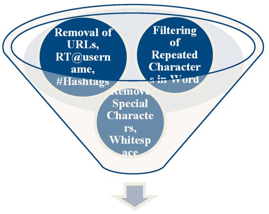
Figure 3.
Structure for preprocessing user tweets on Twitter.

Table 4.
Algorithm for preprocessing of Twitter linguistic data.
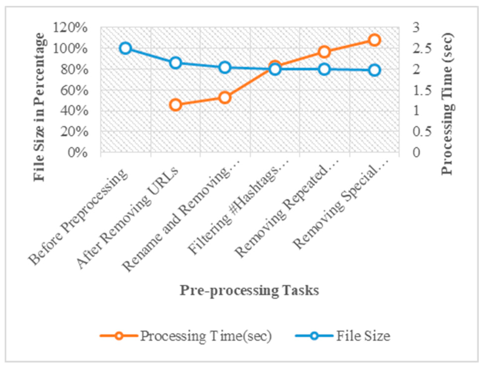
The second step to perform preprocessing in the given algorithm is to remove “@username” from the tweet. “@username” is the tag with “@” followed by the user id or the user name on Twitter platform. In this process, a two-step approach was used to eliminate RT “@username” from the tweet. First, the words “@username” were replaced by “AT_USER” and then by finding patterns “RT + AT_USER” in the sentence and replacing them with the blank character, these words were removed from the dataset. This preprocessing step reduces the size of the dataset as well as eliminates the information that does not contain sentiment or emotional meaning to it. In step 3, the “#” or “hashtag” symbols are removed from the tweet. Therefore, special characters are removed from the sentences, and, in Step 4, repeated characters in the words are removed to obtain the sentimental meaning from words in the sentence. Preprocessing the tweets removes the noise and reduces the size of the dataset as shown in Figure 4. As a result, the filtered data can achieve high performance in analyzing data when the machine learning algorithm is trained. The size of the dataset is reduced and matched after each preprocessing step. Table 5 shows the reduction in file size after each preprocessing step. The reduction and cleaning of the data allow the other natural language processing tasks to be performed with high performance and accuracy.
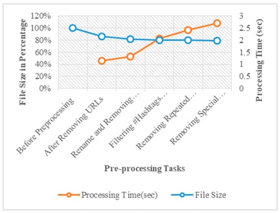
Figure 4.
Reduction in file size after each preprocessing task.

Table 5.
Analysis of file size and data processing time using derived algorithm.
Table 5 shows the raw tweet data from period 8 to 9 June 2014 which has 24,336 raw tweets and the size of.csv file as 4308 KB. After removing URLs from the data, there was a significant drop in the size of the dataset to 3695 KB (85.77%). It shows the noise in the Twitter data consisting of URLs in tweets that do not contribute to the sentiments in the data. The processing time for filtering URLs from the dataset took 1.15 seconds. Further, to process sentence analysis, all the words that contained tag “RT” followed by “@username” were eliminated. This reduced the size of the dataset to 3518 KB (81.66%) in comparison to the original dataset.
Further, #Hashtags were filtered from the dataset followed by the word which may give us sentiment meaning to the word(s). It took 2.60 s to filter the #Hashtags from the dataset. Once applied, the size was reduced to 3442 KB (79.90%). The reduced size of a 3420 KB (79.39%) dataset was obtained after preprocessing and filtering, which means approximately 888 KB of noise was eliminated from the raw text.
As shown in Figure 4, the file size decreased when we filtered the data by applying preprocessing steps. The maximum time taken is 2.70 s for filtering special characters and 2.42 s for filtering repeated characters. Additionally, a pattern-matching task can be performed and due to a large number of duplicate characters in the dataset, it might take a longer time to process thereby increasing the load on the processor. From Figure 4 it can be observed that there was a reduction in dataset size by 20% by removing URLs, RT@username, and #Hashtags from the tweets. Moreover, it gives us a cleaner dataset after filtering the tweets using preprocessing steps. Natural language processing (NLP) can be applied for sentiment analysis on the clean data for better efficiency and accuracy.
4. Linguistic Data Processing Using Natural Language Processing (NLP)
Processing of natural language can be categorized in two ways: firstly, by logically thinking and writing, and secondly, logically thinking and verbally communicating. Moreover, the term “logically thinking or understanding” is defined as “natural language processing”, which we process in our mind logically as a human, and a computer performs using instructional steps written in programming language through central processing units (CPUs). Therefore, the term natural language processing involves a comprehensive set of techniques that allows automatic generation, manipulation, and analysis of natural human languages.
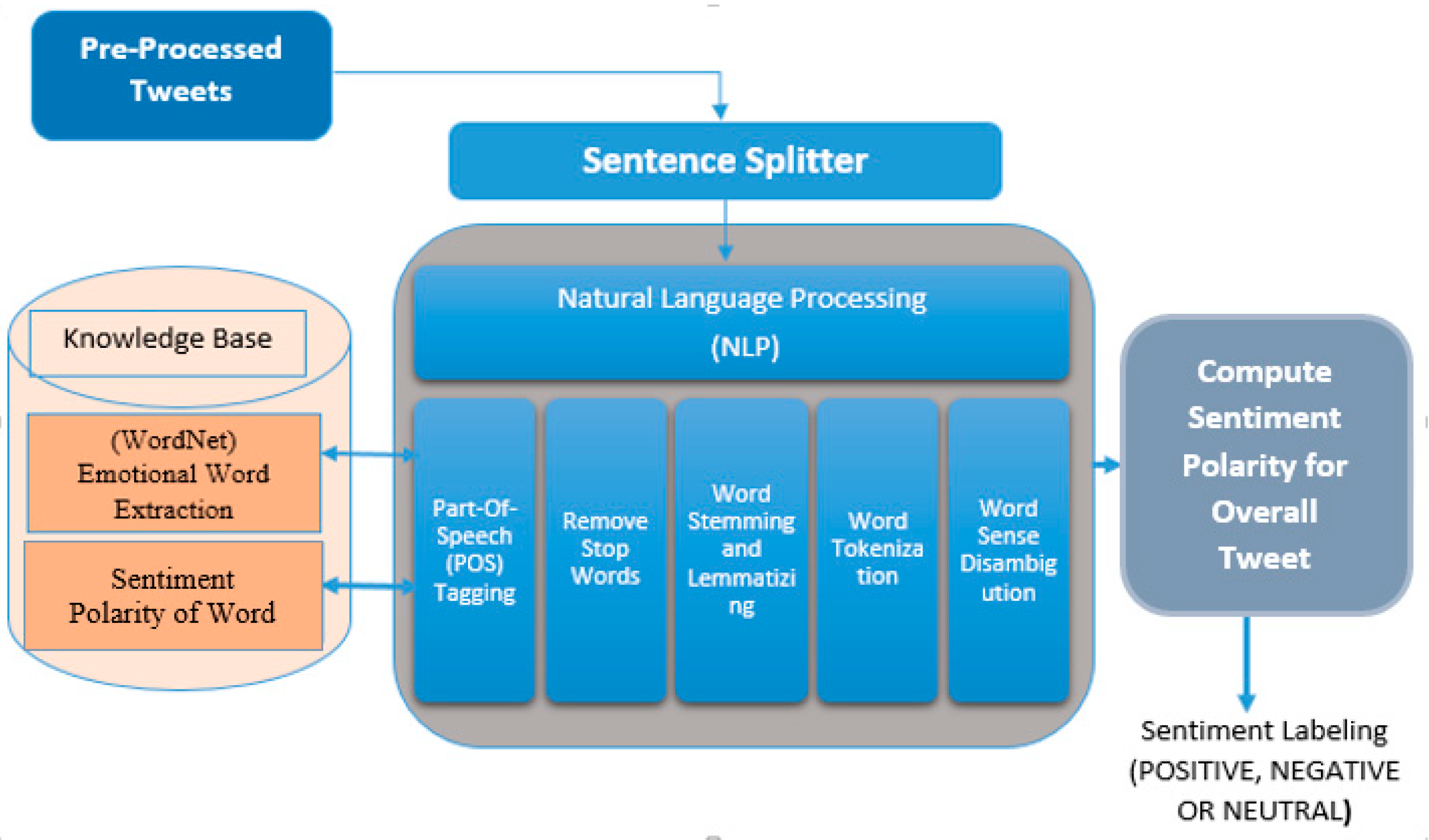
Using natural language processing (NLP) steps, one can process a large amount of non-structured data by analyzing sentence structure, and can compute sentence- or document-level sentiment polarity with the use of famous linguistic databases or lexical resources like WordNet, SentiWordNet, and treebanks [2]. The techniques involved in processing natural language are part-of-speech POS tagging, parsing, named entity recognition, information extraction, word sense disambiguation, word stemming and lemmatization, stop word analysis, word tokenization, and many others depending upon the research objective. During the evaluation process, punctuations between the lines are noted carefully and the expressions that are either idiomatic or colloquial are recognized, which helps in clarifying and understanding the “negations” that revises the word’s polarization depending upon the various types of parts of speech (nouns, prepositions, adverbs, pronouns, adjectives, interjections, conjunctions, and verbs) by taking into consideration the particular “functional-logic” statements [1]. This approach used for analyzing sentiment from linguistic data is known as a lexicon-based or dictionary-based approach. The derived architecture for sentiment analysis using natural language processing (NLP) is shown in Figure 5.
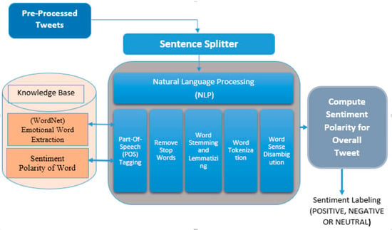
Figure 5.
Derived architecture for sentiment analysis using natural language processing (NLP).
Here, a knowledge-based tool is developed as shown in Figure 5 that analyzes each word in the context, and finds the related synsets (synonyms of word) and lemmas (head words) to achieve accuracy in the sentiment score obtained from the tweets.
A. Word Tokenization
After filtering the noise from that dataset, all that was left were raw words in the sentences. These words individually have some meaning and may consist of emotion or sentiment expressed by the user in the tweet. In natural language processing, the process or steps for breaking down sentences into words and punctuation marks is known as tokenization [2]. The goal for generating the list of words by separating the string is called tokenizing sentences into words [15]. Here, to tokenize the words, the Natural Language Toolkit (NLTK) tokenize package Tweet Tokenizer module is used. The choice for selecting tokenizer depends on the characteristic of data and the language. The algorithm for word tokenization using Tweet Tokenizer is shown in Table 6.

Table 6.
Algorithm for word tokenization.
B. Word Stemming
Stemming and lemmatizing of words are used to produce the normalized form of a word [16] in the text. According to reference [5], word stemming is a technique that gets the root (base) of the word in the text. It normalizes the word by removing the suffix from the word, which gives the root meaning of the word. In this approach of data preprocessing, the Porter stemmer algorithm is used for stripping a suffix from the word to retrieve the proper meaning from the text. Porter stemmer algorithm originally was published by M.F. Porter [16], and the algorithm was developed using Basic Combined Programming Language (BCPL) for removing a suffix from the word automatically and it gives the root meaning to the word in text by removing various suffixes like –ed, -ing, -ion, and -ions by stemming methodology and gives more abstract meaning to the word [17]. Porter stemmer stems the word, character by character, and removes the suffix and gives the base meaning to the word. To achieve accuracy in sentiment analysis, only stemming the word whose length is greater than two, as words like “a”, “is”, “an”, and “the” are not taken into consideration when applied to the sentiment dictionary for getting polarity of the word. The algorithm for performing word stemming is shown in Table 7. The returned stemmed word will be in a more generic form (e.g., the words like “connected”, “connecting”, “connects” stemmed to the single word “connect”, which is the more generic form of the word) and can be used in the further steps of a natural language processing task.

Table 7.
Algorithm for word stemming and lemmatizing.
C. Word Lemmatization
It is a technique that transforms the structural form of a word to the base or dictionary form of a word by filtering the affixation or by changing a vowel from the word. The outcome achieved from the word is known as lemma [18]. Lemmas are the word that has a root meaning of the term requested and the lemmatized word is the gateway to the WordNet [19]. Therefore, lemmatizing the word using an algorithm will create a lemma which will further pass to the WordNet dictionary that pulls out the sense of the word and its sense number, which is the objective for getting a better sentiment score for the word. Lemmatizing words by matching character by character is done through the “WordNetLemmatizer” class available through WordNet class of stem package in Python NLTK. To achieve an effective lemma or root meaning of the word using WordNetLemmatizer, it is really important that the input word must be passed in lower case to the WordNetLemmatizer algorithm to achieve accuracy. Therefore, the lowercase word is passed to the function, which is greater than two in length to retrieve an effective lemmas word from WordNetLemmatizer class (e.g., word “women” is lemmatized to form “woman”, which is a root meaning in the WordNet dictionary).
D. Removing Stop Words
While processing natural language, some of the words which have high occurrence in the document are stop words (e.g., “and”, “the”, “am”, “is”), which only have little emotional meaning and they do not affect the sentiment score when applied to lexical resources. According to reference [19], in their experiment, they compared both the results of keeping the stop words in the text as well as filtering stop words from the text. The result obtained has high accuracy in sentiment classification for keeping stop words as is in the document. Therefore, keeping the idea of reference [20], both the approaches to compare sentiment classification, with and without stop words in the tweets, were taken into consideration. Therefore, the stop words like “I”, “am”, “with”, “and”, “it’s”, “each”, “other”, and “with” are filtered from the tweets.
E. Part-of-Speech (POS) Tagging
This technique annotates the part-of-speech (e.g., noun, adverb, adjective, subjects, objects) to the words, analyzing the sentence structure, and creates the raw form of word sense disambiguation [12]. According to reference [21], it is the last step in natural language processing for analyzing the sentiment score from the sentence. By performing this step, one can obtain featured words that represent the sentence structure and the meaning of the words in the domain it belongs to in the sentence. To achieve annotated part-of-speech in the approach used, the POS tagger class available in the NLTK package was used to develop an algorithm and to obtain word sense for only English language tags from the sentence. It analyzes the lowest level of syntactic structure of the sentence and tags them with their related part-of-speech (e.g., “NN-NOUN”, “IN-Proposition or subordinating conjunction”, “NNP-Proper Noun singular” etc.), which categorizes the word lexically with its POS label and glosses together for further classification. After tagging part of speech to each word in the sentence, it is necessary to structure the sentence in order to achieve accuracy in sentiment polarity for the sentence. As a result, it will affect the accuracy in assigning the sentiment polarity to the sentence, i.e., positive, negative, or neutral.
As an example, the sentence “I do not like to watch this game it is not interesting” contains the phrase “do not”, “not” is the negation word, which changes the meaning of the sentence. To solve this problem, the meaning of the word is changed to the opposite (antonym of word) meaning, if the word is followed by a negation word. In the sentence “I do not like to watch this game, it is not interesting” the word “like” will be replaced by “dislike” and the word “interesting” will be replaced by “uninteresting”. Hence, to analyze this sentence using lexical resources (like SentiWordNet or WordNet Affect), it will provide a higher total negative sentiment score for the sentence. Therefore, to achieve accuracy in sentiment analysis, we developed an algorithm shown in Table 8 that reverses the sentiment score, if the word(s) sense in the sentence refers to negative meaning (for example: “do not”, “not”, “did not”, “cannot”) and occurrence of such words in a sentence. The algorithm takes negation words into account for the analysis, which refers to the mark negation module available in sentiment utility under the NTLK package.

Table 8.
Algorithm for marking negation words.
This method assigns the “_NEG” tag for the words which are followed by the negation words. During the sentence analysis, if the words like “not”, “didn’t”, and “do not” appear in the sentence, all the words until the last word of the sentence are classified with tag “_NEG”. The result of the first step is stored in the list for further analysis, and will further provide a negation score (1 or 0) to the word. In the second step, by iterating the results obtained in the first step and parsing the word with the tag “_NEG” the score ‘1’ is assigned to the negation tagged word and “0” to the word without a tag. The word with score “1” will return the list of lemmas that contains the antonym to the original word and will reverse the meaning as well the polarity of the sentence when applied to the lexical resources to achieve accuracy in sentiment analysis from the Twitter data. Table 9 displays the functioning of algorithm steps as described above.

Table 9.
Example of marking negation word.
4.1. Computing Sentiment Polarity
An algorithm was developed to find the correct synset from a given word and then the part-of-speech was used to obtain the most accurate sentiment score when applied to lexical resources. This interconnection of semantic and lexical relationship for the words and their meanings are known as synsets or synonyms set or group of synonyms. The algorithm in Table 10 finds accurate synsets (all synonyms), lemmas (head words), and antonyms, as well as the part-of-speech (POS) tag which most accurately relates to the term. The WordNet form of the lexical database was used to label the synsets, lemmas, antonyms, and POS from the given tweets. The WordNet form of the lexical databases is commonly used by the dictionary- (lexicon) based approach, which automatically generates the dictionary of the words and its relationship in proper size. According to reference [22], the WordNet database consisted of 150,000 words which were organized in over 115,000 synsets. The synsets resulted in 207,000 pairs of word senses in the year 2006. The book by Bird et al. [2] mentions that the WordNet lexical resource contained 155,287 words and 117,659 synset (synonyms set) records by the year 2009.

Table 10.
Algorithm extract emotional words from tweet.
Once all the synonyms and the antonyms are obtained from the selected lemma names, negation marks are added to the lemma names as shown in the second step of Table 9. When the negation mark is 1, it will return antonyms for the given lemma in synset with its POS tag and if the negation mark is 0, it will return the most accurate synonyms for the lemma and POS tag. WordNet lexicon assigns the expressions, positioning the semantic meaning to the lemma, and prepares the information in the context for further identifying the accurate sentiment polarity of the word which conveys its specific emotional content. The extracted opinionated term from the WordNet database is assigned a numerical score using the SentiWordNet dictionary. SentiWordNet is a resource that consists of opinion information for the word extracted from the WordNet database where each term is assigned its numerical scores that contain sentiment value for the word and the gloss (information) associated with the word [23]. It has been constructed with information attached to the synset term, which is built on a quantitative analysis concept and it denotes the vector representation via semi-supervised synset classification methods [24].
In order to explore the words from the tweets and to evaluate emotional words and their relationships using the WordNet object, NLTK is used by importing the WordNet class from the “nltk corpus” module. The WordNet dictionary returns synonyms (synsets) or the antonyms for the word, part-of-speech (POS), and its sense number for the requested corpus. Firstly, it sanitizes the word’s part-of-speech to standardize the POS tags for WordNet. To do so, a method that sanitizes the part-of-speech has been developed that places all POS tags starting with the letter “V” to “WordNet Verb”, “N” to “WordNet NOUN”, “J” to “WordNet ADJECTIVE”, “R” and “A” to “WordNet ADVERB” and others were tagged to “NONE”. The results of the sanitization of the POS tags are shown in Table 11.

Table 11.
Example of word sanitization.
Further, in the next step of the algorithm in Table 10, the possible synset terms were obtained for the given word and analyzed by iterating through the loop and finding a correct lemma for the given word in the synsets using the WordNet database. After performing the processing of the word and POS tag to obtain synsets, the list of analyzed synset terms obtained is shown by the example in Table 12.

Table 12.
Example of WordNet synset.
All the synsets were analyzed and lemmas were obtained by parsing the synset. The lemmas are the head words or the domain of the word from which it belongs to and contain additional information like part of speech and sense definition [2]. The example in Table 13 shows the list of lemmas for the synset of the word (e.g., “good”) that contains the lemmas from all the domains it belongs to. Here, the last expression or the term in the lemmas is the lemma’s name, which compares the lemma name to the input word. Once the lemma’s name matches the requested (input) word, it is appended to all possible synonyms or antonyms for the matched cases and the sentiment score is obtained.

Table 13.
Example of word lemmas.
Once all the synonyms and the antonyms for the lemmas are obtained, the lemma is selected based on the negation mark. If the negation mark is 1, it will return antonyms for the given lemma in synset with its POS and if the negation mark is 0, it will return the most accurate synonyms for the words and POS tag.
Therefore, the synset term is obtained based on the negation mark and the most accurate lemma’s name with its POS tag that gives an accurate sentiment score when applied to the SentiWordNet database. The sentiment score obtained for all the related terms or words with its POS tag followed by sense number has its “PosScore” and “NegScore” tagged for each word associated with every synset term. The evaluated positive and negative term score from the SentiWordNet dictionary is to determine sentiment orientation for each term in the sentence or tweet. In this approach, firstly, list the sentiment score for the first synset in the synsets list. The score obtained for each synset term is based on the context or the occurrence in the given sentence. An example of a sentiment score calculated for a tweet is illustrated in Table 14.

Table 14.
Assigning sentiment polarity to a word.
The evaluated positive and negative term score from the SentiWordNet database determines the sentiment orientation for each term in the sentences or tweets. In this approach, firstly list the sentiment score for the first synset in the synsets list. The score obtained for each synset term is based on the context or the occurrence in the given sentence. Equation (1) calculates the total positive score (TotalPosScore) and total negative score (TotalNegScore), where n is the number of terms, and t denotes the tweet.
Each tweet that sums up the total positive score and total negative score is then compared for labeling the sentiment as “positive”, “negative”, or “neutral”. Equation (2) gives the overall sentiment polarity Polarityswn(t) for the tweet t.
The sentiment score Polarityswn(t) obtained for the tweet t using the SentiWordNet database provides three measures that determine the sentiment of the user tweet t. The tweet t is positive or 1 if the total positive score is greater than the total negative score; if the total negative score is greater than the total positive score, the overall sentiment is negative or −1, else it is neutral or 0 as shown in Table 15.

Table 15.
Example of output for sentiment analysis.
Finally, the analyzed data file is appended with three additional attributes namely, PosScore (positive score), NegScore (negative score), and the sentiment label. The sentiment label can be either “positive”, “negative”, or “neutral”, defining the sentiment prediction of the user tweet. The dataset obtained after appending the three attributes has a total of nine attributes (Table 3 shows the attributes before appending).
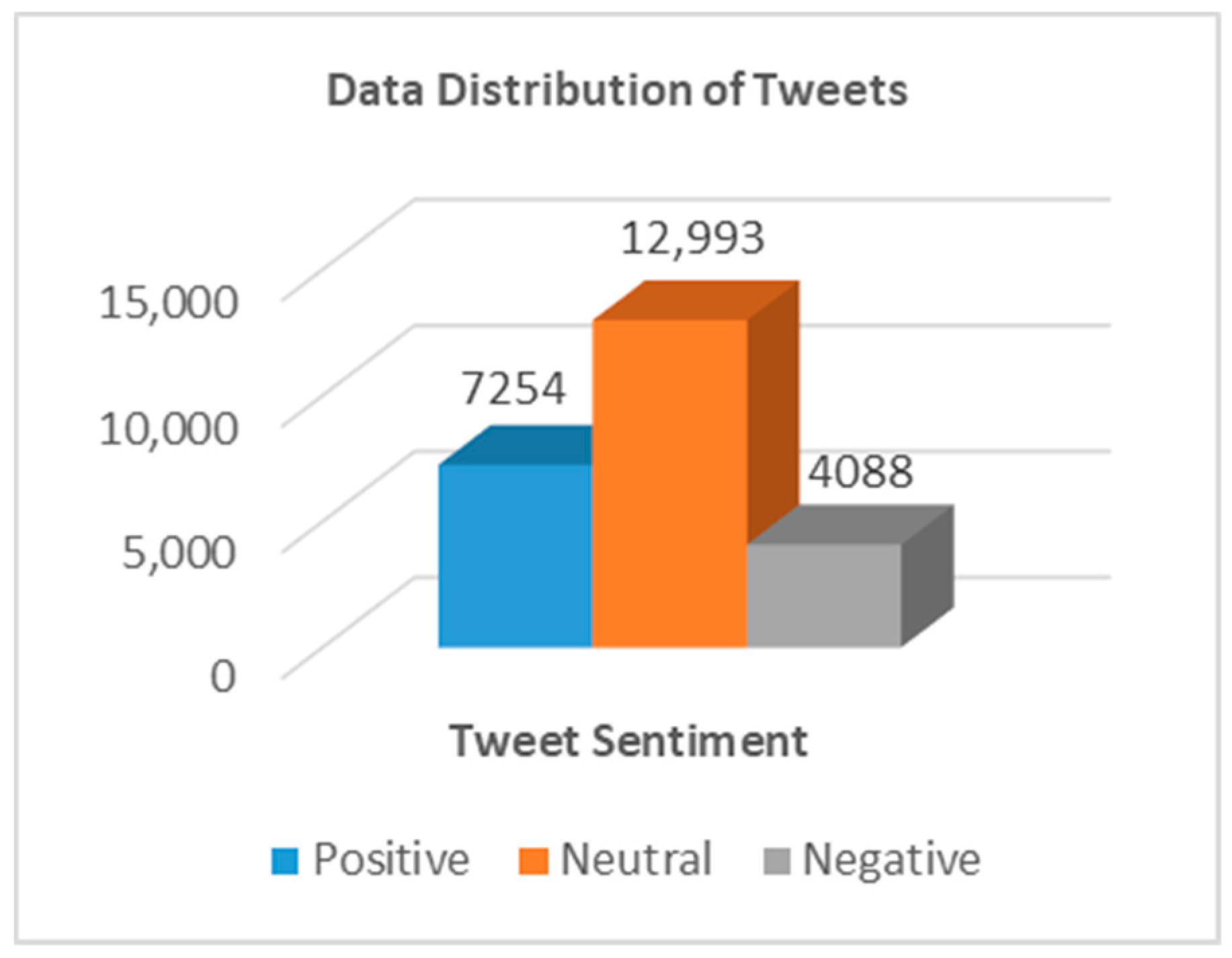
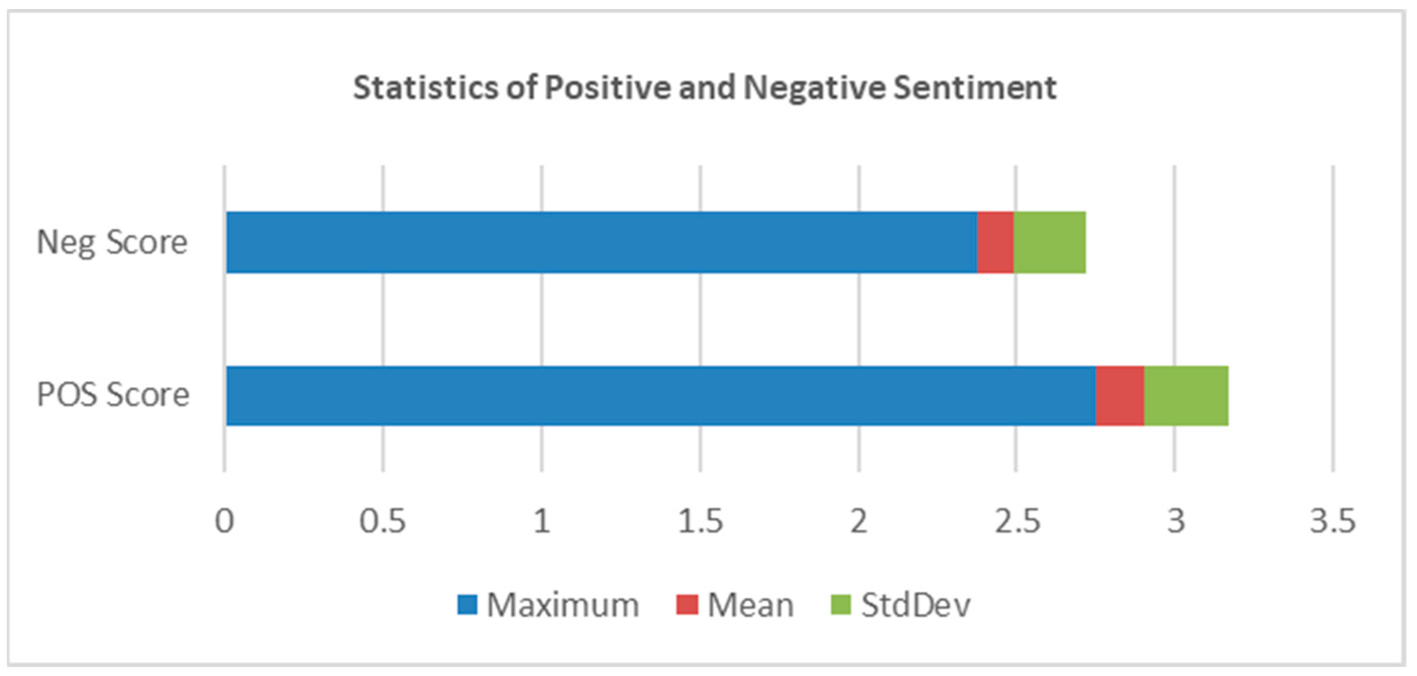
Figure 6 shows the distribution of the data into positive, negative, and neutral tweets. Figure 6 shows 24,335 tweets classified into 7254 positive tweets; 12,993 neutral tweets; and 4088 negative tweets. The number of neutral tweets is higher than the number of positive and negative tweets as only English language tweets were analyzed and the tweets in other languages were ignored. However, the response toward the promotion of the World Cup 2014 was more positive sentiment as opposed to negative sentiment. The positive sentiment of the people towards the event is helpful to the investors and the organizers in taking valuable decisions in promoting the event based on people’s feedback, likes, and dislikes. Figure 7 shows the statistical analysis of the overall sentiment with maximum, mean, and standard deviation of the positive scores and the negative scores.

Figure 6.
Data distribution of tweets.
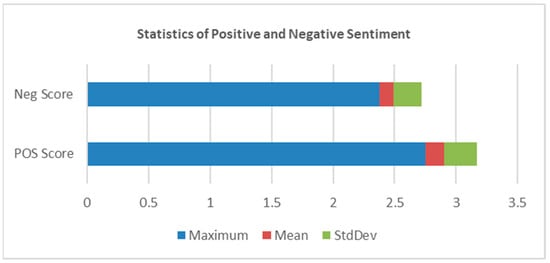
Figure 7.
Statistics of overall positive and negative sentiment tweets.
The maximum positive sentiment score evaluated for the tweets is 2.75, which is the most positive sentimental tweet in the dataset of World Cup 2014 promotion. The tweet which was given a maximum positive score is “Contact with nature is good for health. Come to the #EarthPortal and discover the wonders of the South of #Brazil! #Brazil2014” tweeted by the username “portaldaterra”. The most negative sentiment scores were observed between 0.246 to 0.273 which are accounted for by 2533 negatively classified tweets. The maximum negative sentiment score is 2.375 as seen in Figure 7. In the next section, we discuss machine learning techniques for sentiment analysis.
4.2. Machine Learning Techniques for Sentiment Analysis
A machine learning classifier was trained on the dataset obtained after the sentiment label is computed as discussed in Section 4. Classification performance was measured on the test dataset obtained by the natural language processing task. Naïve Bayes, SVM (support vector machine), KNN (K-nearest neighbor), and random forest algorithms were applied to measure the accuracy and performance metrics for the sentiment-labeled data obtained by processing the Twitter linguistic data using natural language processing (NLP) techniques and assigning sentiment score and polarity to the dataset. The most abstract view that performs sentiment analysis using machine learning is shown in Figure 8.
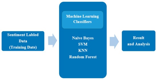
Figure 8.
Overview of applying machine learning. SVM—support vector machine, KNN—K-nearest neighbor.
The software WEKA 3.8 [25] was used for training and testing the classifiers and measuring the performance of the classifiers. The classification of the data was performed by splitting the dataset into training and testing ratios of 90:10, 80:20, 70:30, and 60:40 with 10-fold cross-validation. The 10-fold cross-validation is used to avoid overfitting of the data by the classifiers.
Naïve Bayes
Naïve Bayes is the most commonly used classifier in natural language processing (NLP). The main advantage of this classifier is its simplicity as well as the prediction of the correct class for a new instance [26]. The probability calculations for each hypothesis are simplified for the instances in the class (e.g., positive, negative, and neutral).
In the derived dataset, a given class is Y (positive, negative, and neutral), where X is the instance defined by a feature vector {X1, X2, …, Xn} with n being the number of features (sentiment labels) in the Dataset. Therefore, Bayesian probability of the given class Y with an instance X can be computed P(Y|X) using the following Equation (3) [26]:
where:
- X: instance of class (sentiment labels for each tweet)
- Y: sentiment class (positive, negative, or neutral)
- P(X|Y): instance occurred in particular class for each value of Y (class-conditional density)
- P(Y): prior probability of class
Using Equation (3), we have P(Y|X), the Bayesian probability classification for the class Y to the instance X, which is equal to the probability P(X|Y) for the particular instance being seen under specific class. In this case, the probability of each instance (sentiment labels) belongs under a specific class (positive, negative, or neutral). Further, it is multiplied with the prior probability of the class P(Y). At last, the result obtained is normalized so that the final probability for the given class with its instances will sum up to 1.
Support Vector Machine (SVM)
It is a supervised learning method that produces a mapping function from the available training dataset [27]. Support vector machine (SVM) is widely applied for classification problems and nonlinear regression, which classifies both linear and nonlinear [27]. The mapping function can be the classification function that classifies the labeled data in the dataset. According to reference [28], SVMs are universal learners, which can be used to learn polynomial classifiers and have the ability to learn independent of the dimensionality of the feature space. SVM is very useful in dealing with questions related to the classification of texts by linearly separating them as suggested by reference [28]. One of the disadvantages of using SVM is that it is incapable of differentiating between words that have different senses in different sentences and as a result, particular “domain-based lexicons” cannot be generated [28].
Random Forest
Random forest is a method used to create predictive models for classification and regression and is also known as random forest decisions. A number of decision trees are classified on different sub-samples for the chosen datasets and are fitted into a meta estimator known as random forest [29]. In reference [29], the resultant class is derived based on the majority voting from the generated classes by similar sub-sampled trees generated as the output of the random forest. A random forest classification improves the precision of the forecast and over-fitting control on average and as an ensemble method uses different learning models to produce effective predictive outcomes.
KNN (K-Nearest Neighbor)
K-nearest neighbors (KNN) is a lucid and easy-to-implement algorithm. This algorithm searches for the predefined samples from the training dataset by determining the close proximity for similar things. In other words, similar things are assumed to be close to each other. The distance between the sample space and the query is calculated by selecting the specified number of samples (K) closest to the query and then by evaluating for the most common label (during classification on sentiment labels tweets) or label average (in the regression case). When KNN is used for regression, the prediction is done on the basis of their mean or median values [29]. The output with the highest frequency of identical instances determines the class using KNN classification. Each instance is considered a vote for that class and the class with the most votes determines the sentiment polarity of the prediction class.
5. Results and Discussion
Various performance measures, namely, accuracy, area under the receiver operating characteristics (ROC) curve, recall, false positive rate, precision, and F-measure were used to analyze the results of the classification algorithms naïve Bayes, SVM, random forest, and K-nearest neighbor. The definitions of the measures are given in Equations (4)–(8). Let TPA be the number of true positives of the class A (positive sentiment), TPB be the true positives of the class B (neutral sentiment), and TPC be the number of true positives of class C (negative sentiment). Then, the accuracy can be defined by Equation (4).
The area under the ROC curve (AUC) is a plot of true positive rate (TPR, or specificity) against false positive rate (FPR, or sensitivity).
The true positive rate (TPR), sensitivity, or recall is the number of sentiment labels predicted positive that are actually positive. Recall is defined by Equation (5).
The false positive rate (FPR) is the number of sentiment labels predicted positive that are actually negative and is defined in Equation (6).
Precision is the proportion of the predicted positive cases that were correct. The precision can be calculated using Equation (7).
The F-Measure score is the harmonic mean of the precision and recall. This evaluates the equivalency between the sensitivity (recall) and the precision (correctness) of the data. This gives us the interpretation of how the measure recall and precision values behave for the dataset. The F-measure can be calculated using Equation (8).
Table 16 shows the performance for the sentiment analyzed tweets or labeled tweets for naïve Bayes, SVM, random forest, and K-nearest neighbor classifiers using training-to-testing ratios 90:10, 80:20, 70:30, and 60:40 with 10-fold cross-validation.

Table 16.
Performance results for sentiment analyzed tweets.
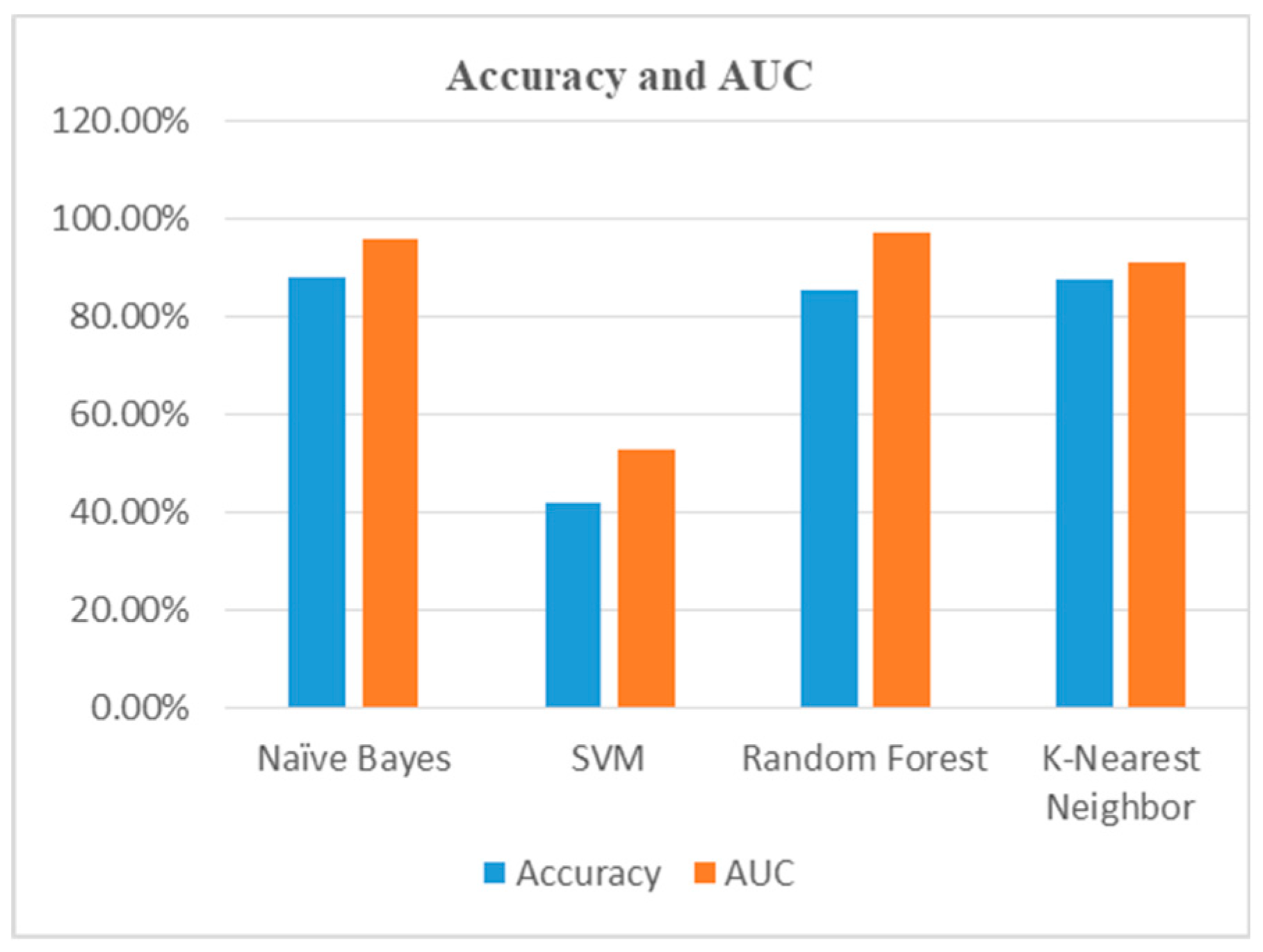
Table 17 shows the confusion matrix for the naïve Bayes classifier. It can be observed that 21,456 sentiment-labeled tweets are correctly classified with just 11.83% (2879) incorrectly classified tweets using a training-to-testing ratio of 90:10 with 10-fold cross-validation. The prediction of sentiment classes positive, negative, and neutral using the naïve Bayes classifier has an accuracy rate of 88.17%. The TP rate for positive, neutral, and negative tweets is 0.821, 0.960, and 0.739, respectively. The weighted average of the TP rate is 0.882. This observation shows that the dataset classified is sensitive, which belongs to the actual class. The FP rate for the positive, neutral, and negative tweets is 0.022, 0.191, and 0.016 respectively. From the data, one can conclude that the classification of the sentiment label has a minimal number of tweets that are incorrectly classified. The precision for the positive, neutral, and negative tweets is 0.941, 0.852, and 0.900, respectively and the weighted average for precision is 0.89. The F-measure for the positive, neutral, and negative tweets are 0.877, 0.903, and 0.812, respectively and the weighted average for the F-score for the classes A, B, and C is 0.88. The AUC for the positive, neutral, and negative classes is 0.966, 0.958, and 0.946 respectively.

Table 17.
Confusion matrix for sentiment class (naïve Bayes).
Table 18 shows the confusion matrix for estimation of the predictive performance of the SVM classifier for a training-to-testing ratio of 90:10 with 10-fold cross-validation giving the best performance of classifying sentiment analysis for tweets. An accuracy of 41.77% is obtained where 10,157 sentiment-labeled tweets are correctly classified and 14,178 sentiment-labeled tweets are incorrectly classified. A recall of 0.417, an FP rate of 0.364, a precision of 0.431, an F-measure of 0.398, and an AUC of 0.527 were obtained for SVM, which is the lowest among all classifiers. It shows that SVM is not able to classify the tweets accurately.

Table 18.
Confusion matrix for sentiment class (SVM).
Table 19 shows the confusion matrix for the estimation of predictive performance by random forest classifier for a training-to-testing ratio of 60:40 with 10-fold cross-validation which gives the best performance in classifying sentiment analysis for tweets. An accuracy of 85.32% was achieved with 20,763 sentiment-labeled tweets correctly classified and 3572 sentiment-labeled tweets incorrectly classified. The diagonal counts show the correctly classified tweets for the positive, neutral, and negative classes in the confusion matrix. A recall of 0.853, an FP rate of 0.127, a precision of 0.853, an F-measure of 0.840, and an AUC of 0.970 were obtained for random forest. It can be observed that random forest gives the best performance among all the classifiers.

Table 19.
Confusion matrix for sentiment class (random forest).
Table 20 shows the confusion matrix for the estimation of predictive performance by KNN classifier for training-to-testing ratio of 80:20 with 10-fold cross-validation which gives the best performance in classifying sentiment analysis for tweets. An accuracy of 87.49% was achieved with 21,290 sentiment-labeled tweets correctly classified and 3045 sentiment-labeled tweets incorrectly classified. The diagonal counts show the correctly classified tweets for the positive, neutral, and negative classes in the confusion matrix. A recall of 0.875, an FP rate of 0.085, a precision of 0.874, an F-measure of 0.875, and an AUC of 0.911 were obtained for KNN.

Table 20.
Confusion matrix for sentiment class (KNN).
Different machine learning techniques were used for training the sentiment-labeled dataset and the results obtained using the classifiers vary using different classifiers. The performance evaluation of the classification results obtained using naïve Bayes, SVM, random forest, and KNN supports the objective for processing a linguistic dataset using natural language processing (NLP) techniques and measuring the accuracy and AUC of the sentiment-labeled dataset. Comparing different classifiers for measuring the accuracy and AUC for the sentiment-labeled dataset, naïve Bayes and KNN algorithms give the highest accuracy with random forest giving the best AUC in data classification. Table 21 shows accuracy and AUC using different classifiers and Figure 9 shows the graphical analysis for the combined results.

Table 21.
Combined result analysis.
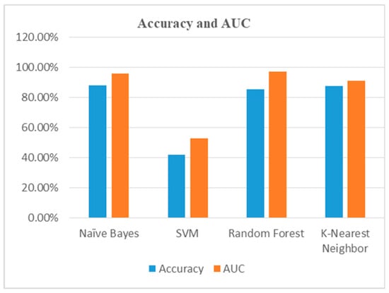
Figure 9.
Graphical results analysis.
The objective of combining lexicon-based and machine learning methods for sentiment analysis of Twitter data shows that using natural language processing (NLP) techniques gives an accurate classification for a linguistic dataset.
6. Conclusions and Future Work
In this paper, a unique approach to perform sentiment analysis on a linguistic dataset was introduced using machine learning algorithms. The developed algorithms for removing noise or data filtering and preprocessing linguistic data using natural language processing (NLP) techniques were demonstrated. The preprocessing of the input tweets was filtered and processed to give more accurate data as well as to reduce the size of the dataset. Work tokenization, stemming, lemmatization, and part-of-speech (POS) were used to find sentiment scores for the tweets. Further analysis of data using machine learning algorithms like naïve Bayes, SVM, random forest, and KNN was applied for classifying the tweets as positive, neutral, or negative sentiment and the performance of the classifiers was measured for accuracy and reliability of the classified sentiment analysis. The results show the usefulness and efficiency of the techniques used and described in the paper.
For the future work on sentiment analysis, it would be useful to perform real time sentiment polarity assignment to the Twitter data. The implementation could be performed on the cloud that would increase the performance efficiency for sentiment analysis using natural language processing (NLP) techniques. This can be done by creating nodes on a cloud data platform like Hadoop that allow us to store the data on the cloud using the Hadoop File System (HDFS) and map-reduce concept to distribute the data processing algorithm to load and process large size datasets, and real time sentiment analysis for the linguistic data can be performed. This will be the contribution towards real time sentiment analysis in a cloud environment and will allow the business users to determine real time sentiment analysis for the linguistic data.
Author Contributions
Conceptualization, K.P.; Data curation, R.P.; Formal analysis, K.P. and R.P.; Investigation, K.P. and R.P.; Methodology, K.P. and R.P.; Project administration, K.P.; Resources, K.P. and R.P.; Software, R.P.; Validation, R.P.; Visualization, R.P.; Writing—original draft, R.P.; Writing—review and editing, K.P. All authors have read and agreed to the published version of the manuscript.
Funding
This research received no external funding.
Conflicts of Interest
The authors declare that they have no known competing financial interests or personal relationships that could have appeared to influence the work reported in this paper.
References
- Neri, F.; Aliprandi, C.; Capeci, F.; Cuadros, M.; By, T. Sentiment analysis on social media. In Proceedings of the 2012 International Conference on Advances in Social Networks Analysis and Mining (ASONAM 2012), Istanbul, Turkey, 26–29 August 2012. [Google Scholar]
- Steven, B.; Klein, E.; Loper, E. Natural Language Processing with Python; O’Reilly Media, Inc.: Newton, MA, USA, 2009. [Google Scholar]
- Twitter. Available online: https://about.twitter.com/company (accessed on 30 June 2019).
- Olsson, F. A Literature Survey of Active Machine Learning in the Context of Natural Language Processing. Available online: https://www.semanticscholar.org/paper/A-literature-survey-of-active-machine-learning-in-Olsson/abebd207b1cf56ced502b0bb203d1f231b58d699 (accessed on 1 April 2009).
- Eman, M.G.Y. Sentiment Analysis and Text Mining for Social Media Microblogs using Open Source Tools: An Empirical Study. Int. J. Comput. Appl. 2015, 112, 44–48. [Google Scholar]
- Firmino Alves, A.L.; Baptista, C.D.S.; Firmino, A.A.; Oliveira, M.G.D.; Paiva, A.C.D. A Comparison of SVM versus naive-bayes techniques for sentiment analysis in tweets: A case study with the 2013 FIFA confederations cup. In Proceedings of the 20th Brazilian Symposium on Multimedia and the Web, João Pessoa, Brazil, 18–21 November 2014; ACM: New York, NY, USA, 2014. [Google Scholar]
- Hemalatha, I.; Dr GP Saradhi, V.; Govardhan, A. Case Study on Online Reviews Sentiment Analysis Using Machine Learning Algorithms. Int. J. Innov. Res. Comput. Commun. Eng. 2014, 2, 3182–3188. [Google Scholar]
- Hemalatha, I.; Dr GP Saradhi, V.; Govardhan, A. Preprocessing the informal text for efficient sentiment analysis. Int. J. Emerg. Trends Technol. Comput. Sci. (Ijettcs) 2012, 1, 58–61. [Google Scholar]
- Bandgar, B.M.; Kumar, B. Real time extraction and processing of social tweets. Int. J. Comput. Sci. Eng. 2015, 2347–2693, 1–6. [Google Scholar]
- Augustyniak, Ł.; Szymański, P.; Kajdanowicz, T.; Tuligłowicz, W. Comprehensive Study on Lexicon-based Ensemble Classification Sentiment Analysis. Entropy 2015, 18, 4. [Google Scholar] [CrossRef]
- Isah, H.; Trundle, P.; Neagu, D. Social media analysis for product safety using text mining and sentiment analysis. In Proceedings of the 2014 14th UK Workshop on Computational Intelligence (UKCI), Bradford, UK, 8–10 September 2014; IEEE: New York, NY, USA, 2014. [Google Scholar]
- Bakshi, R.K.; Kaur, N.; Kaur, R.; Kaur, G. Opinion mining and sentiment analysis. Found. Trends Inf. Retr. 2008, 2, 1–135. [Google Scholar] [CrossRef]
- MacArthur, A. The Real History of Twitter, In Brief-How the Micro-Messaging Wars were Won. Lifewire. Available online: https://www.lifewire.com/history-of-Twitter-3288854 (accessed on 11 September 2020).
- Fernández-Gavilanes, M.; Álvarez-López, T.; Juncal-Martínez, J.; Costa-Montenegro, E.; González-Castaño, F.J. Unsupervised method for sentiment analysis in online texts. Expert Syst. Appl. 2016, 58, 57–75. [Google Scholar] [CrossRef]
- Perkins, J. Python Text Processing with NLTK 2.0 Cookbook; Packt Publishing Ltd.: Birmingham, UK, 2010. [Google Scholar]
- Toman, M.; Roman, T.; Karel, J. Influence of word normalization on text classification. Proc. Inscit 2006, 4, 354–358. [Google Scholar]
- Porter Martin, F. An algorithm for suffix stripping. Program 1980, 14, 130–137. [Google Scholar] [CrossRef]
- Liu, H.; Christiansen, T.; Baumgartner, W.A.; Verspoor, K. BioLemmatizer: A lemmatization tool for morphological processing of biomedical text. J. Biomed. Semant. 2012, 3, 1. [Google Scholar] [CrossRef] [PubMed]
- Bhattacharyya, P.; Bahuguna, A.; Talukdar, L.; Phukan, B. Facilitating multi-lingual sense annotation: Human mediated lemmatizer. In Proceedings of the Seventh Global Wordnet Conference, Tartu, Estonia, 25–29 January 2014. [Google Scholar]
- Saif, H.; He, Y.; Alani, H. Semantic sentiment analysis of Twitter. In International Semantic Web Conference; Springer: Berlin/Heidelberg, Germany, 2012. [Google Scholar]
- Kouloumpis, E.; Wilson, T.; Moore, J. Twitter Sentiment Analysis: The Good the Bad and the OMG! In Proceedings of the Fifth International AAAI Conference on Weblogs and Social Media (ICWSM), Catalonia, Spain, 17–21 July 2011; pp. 538–541. [Google Scholar]
- Wawer, A.; Choukri, K.; Maegaard, B.; Mariani, J.; Odijk, J. Is Sentiment a Property of Synsets? Evaluating Resources for Sentiment Classification using Machine Learning. In Proceedings of the Seventh International Conference on Language Resources and Evaluation (LREC’10), Valletta, Malta, 17–23 May 2010; pp. 1101–1104. [Google Scholar]
- Ohana, B.; Tierney, B. Sentiment classification of reviews using SentiWordNet. In Proceedings of the 9th IT & T Conference Dublin Institute of Technology, Dublin, Ireland, 22–23 October 2009. [Google Scholar]
- Esuli, A.; Sebastiani, F. Sentiwordnet: A publicly available lexical resource for opinion mining. In Proceedings of the Fifth International Conference on Language Resources and Evaluation (LREC’06), Genoa, Italy, 22–28 May 2006; Volume 6, pp. 417–422. [Google Scholar]
- Weka 3: Data Mining Software in Java. Weka 3-Data Mining with Open Source Machine Learning Software in Java. N.p., n.d. Web. 03 Jan 2017. Available online: http://www.cs.waikato.ac.nz/ml/weka/ (accessed on 16 July 2019).
- Murphy, K.P. Naive Bayes Classifiers; The University of British Columbia: Vancouver, BC, Canada, 2006; Volume 18, p. 60. [Google Scholar]
- Wang, L. (Ed.) Support Vector Machines: Theory and Applications; Springer Science & Business Media: Berlin/Heidelberg, Germany, 2005; Volume 177. [Google Scholar]
- Joachims, T. Text Categorization with Support Vector Machines: Learning with Many Relevant Features. In European Conference on Machine Learning; Springer: Berlin/Heidelberg, Germany, 1998. [Google Scholar]
- Al Amrani, Y.; Lazaar, M.; El Kadiri, K.E. Random forest and support vector machine based hybrid approach to sentiment analysis. Procedia Comput. Sci. 2018, 127, 511–520. [Google Scholar] [CrossRef]
© 2020 by the authors. Licensee MDPI, Basel, Switzerland. This article is an open access article distributed under the terms and conditions of the Creative Commons Attribution (CC BY) license (http://creativecommons.org/licenses/by/4.0/).

