Review

Machine Learning in Slope Stability: A Review with Implications for Landslide Hazard Assessment

Department of Mining and Geological Engineering, University of Arizona, 1235 E James E Rogers Way, Tucson, AZ 85721, USA
*
Author to whom correspondence should be addressed.
GeoHazards 2025, 6(4), 67; https://doi.org/10.3390/geohazards6040067 (registering DOI)
Submission received: 15 September 2025 / Revised: 4 October 2025 / Accepted: 13 October 2025 / Published: 16 October 2025

Abstract

Slope failures represent one of the most serious geotechnical hazards, which can have severe consequences for personnel, equipment, infrastructure, and other aspects of a mining operation. Deterministic and stochastic conventional methods of slope stability analysis are useful; however, some limitations in applicability may arise due to the inherent anisotropy of rock mass properties and rock mass interactions. In recent years, Machine Learning (ML) techniques have become powerful tools for improving prediction and risk assessment in slope stability analysis. This review provides a comprehensive overview of ML applications for analyzing slope stability and delves into the performance of each technique as well as the interrelationship between the geotechnical parameters of the rock mass. Supervised learning methods such as decision trees, support vector machines, random forests, gradient boosting, and neural networks have been applied by different authors to predict the safety factor and classify slopes. Unsupervised learning techniques such as clustering and Gaussian mixture models have also been applied to identify hidden patterns. The objective of this manuscript is to consolidate existing work by highlighting the advantages and limitations of different ML techniques, while identifying gaps that should be analyzed in future research.

1. Introduction

In recent years, technological equipment production has sped up dramatically for items like processors and graphics cards, batteries, and hybrid vehicles. The rise in technological advancements demands more raw materials such as minerals, which leads to expanded open-pit mining operations and deeper as well as steeper excavations [1]. The stability of these steep slopes presents major geotechnical problems that rely on the interactions between geological formations, rock mass properties, hydrogeological elements, and daily mining operations, such as blasting [2]. Slope stability failures that occur during mining operations can lead to serious consequences, including loss of life, financial damage, and environmental impact. The critical role of slope stability in mining operations drives geotechnical engineers and researchers to continuously develop better analytical methods for evaluating and reducing slope collapse hazards [1].
A clear distinction must be made between soil slopes and rock slopes, as their governing stability mechanisms differ substantially. Soil slopes are typically controlled by shear strength reduction, pore-water pressure buildup, and progressive failure in relatively homogeneous materials. In contrast, rock slopes are primarily influenced by the presence of discontinuities, joint networks, bedding planes, and block interactions, which govern both kinematic and overall stability. Given that mining excavations are often conducted in hard rock formations where these structural features predominate, this review focuses primarily on rock slopes in open-pit mining operations, while acknowledging that some of the discussed methods may also be applicable to soil slope contexts.
The traditional evaluation process for slope stability incorporates both deterministic and stochastic analytical techniques. The Limit Equilibrium Method (LEM), Finite Element Method (FEM), and Finite Difference Method (FDM) deterministic techniques evaluate slope stability based on predefined geotechnical parameters, which consist of soil and rock characteristics along with groundwater pressures and external loading conditions [3]. These methods allow the calculation of the Factor of Safety (FOS), which is an essential value to establish the probability of failure of a slope [4]. Deterministic methods provide important results on slope behavior, but their analytical capability is limited because they cannot represent the variability and uncertainty inherent to natural geological structures. Cohesion, friction angle, and pore water pressure demonstrate significant variations over different locations and time periods, which makes it difficult to establish one typical value for analysis [5].
To address these limitations, researchers have developed probabilistic or stochastic methods that incorporate variability and uncertainty into slope stability analyses. Stochastic methods, such as Monte Carlo simulation and Reliability Index Methods (RIM), use probability distributions to define key geotechnical parameters, in contrast to fixed numerical values [6]. These approaches enable more realistic assessments by considering a range of possible failure scenarios [7]. Bayesian update techniques further improve predictions by integrating in situ measurements and observational data to refine slope failure probability assessments [3]. However, stochastic methods face challenges in modeling complex nonlinear interactions inherent to rock masses and often require considerable computational resources, limiting their applicability in real-time decision-making [8]. These constraints motivate the exploration of alternative approaches that can overcome such limitations.
Advances in computational technologies and data science have enabled the integration of Machine Learning (ML) methods into slope stability assessment, opening new avenues for enhanced prediction accuracy and risk analysis [9]. ML models analyze large geotechnical datasets to identify complex patterns and nonlinear relationships that traditional methods often miss. These models are trained using historical slope failure data, incorporating variables such as slope geometry, material characteristics, hydrological conditions, and environmental factors such as rainfall, to provide robust predictive capabilities. Supervised learning algorithms, including Decision Trees (DT), Support Vector Machines (SVM), Random Forest (RF), Artificial Neural Networks (ANN), and Gradient Boosting Machines (GBM) have demonstrated strong potential in classifying slope stability conditions and estimating the safety factor with high accuracy [10].
Beyond slope stability, Machine Learning techniques have proven applicable in a wide range of geoscience domains, including mineral prospectivity mapping, groundwater modeling, seismic hazard assessment, and landslide susceptibility mapping. These applications illustrate the versatility of ML and suggest opportunities for cross-disciplinary knowledge transfer to enhance slope stability analysis. Ensemble learning models such as Random Forest and XGBoost are particularly valuable, as they improve predictive reliability by combining multiple learners, reducing overfitting while enhancing generalization in geotechnical applications with substantial data uncertainty [11,12]. The analysis of remote sensing and time-series monitoring data has further driven research into advanced deep learning approaches, including Convolutional Neural Networks (CNN) and Long Short-Term Memory (LSTM) networks [13], while unsupervised techniques such as Clustering and Gaussian Mixture Models (GMM) enable the discovery of latent patterns governing slope failure mechanisms [14].
ML-based projects allow for efficient processing and analysis of large data, such as slope deformations or velocities, where data is generated every 2 to 10 s and can be derived from multiple sources, such as geotechnical parameters and InSAR radars [3]. Traditional methods have difficulty incorporating large and varied datasets, whereas ML models demonstrate efficient management of diverse data inputs and rapid adaptation to new information. ML methods allow slope stability to be assessed in re-al-time by continuously adjusting their predictions based on new data collected during mining [9]. Open pit mining operations need this functionality because daily excavation activities, weather conditions, and changes in groundwater levels can rapidly transform slope conditions [15].
Before mining companies fully integrate Machine Learning applications for slope stability analysis into their operations, they must overcome various practical challenges. The quality and accessibility of geotechnical data stand as primary concerns because ML models need precise and detailed datasets to train and validate their systems [16]. In several situations, the lack of or missing historical slope failure data, together with specific geotechnical data on displacements and velocities, leads to limitations that produce biased results in the prediction models [17]. Engineers face significant challenges when interpreting Machine Learning models because different engineers can produce varying results during evaluation. As we know, the algorithms used by Machine Learning to perform the calculations are not easy to understand and require advanced programming knowledge. This often prevents geotechnical engineers and decision-makers from understanding the logic behind their predictions. Decision-making on a safety-critical task such as slope stability requires a clear demonstration of how the results were obtained and what the calculation procedure was, so transparent and explanatory methods remain essential.
Several studies recommend hybrid modeling solutions that combine ML techniques with traditional geotechnical methods for addressing the identified challenges [9]. Finite element simulations can be improved with the addition of ML models, which aid in the optimization of input parameters and more accurate FOS predictions. Model transparency can be increased while the most significant factors contributing to slope stability can be identified by using feature selection techniques along with explainable artificial intelligence (XAI) approaches [18]. Slope stability forecasts are improved by applying uncertainty quantification methods such as Bayesian inference and probabilistic Machine Learning models, which use confidence intervals and probability distributions to better describe the predictions’ level of confidence [12].
This paper reviews ML techniques for slope stability assessment and their efficacy, as well as possible limitations and potential for on-site deployment in mines. We examine a variety of ML methods, including supervised learning techniques, unsupervised learning approaches, and hybrid learning systems. To ensure systematic and comprehensive coverage of the existing literature, this review is based on a structured search of scholarly databases. Articles were retrieved primarily from Scopus and Google Scholar within the timeframe of 2000–2025, reflecting the period of significant growth in computational approaches and Machine Learning applications in geotechnical engineering. Inclusion criteria were restricted to peer-reviewed journal articles that specifically address slope stability analysis in mining or geotechnical contexts. Studies focusing solely on unrelated fields or lacking direct relevance to slope stability were excluded. This methodological framework enhances the reproducibility of the review and ensures that the findings are grounded in high-quality, domain-specific research. The purpose of this study is to give a thorough summary of the state of the art while also evaluating how well it corresponds to real-world use. We assess the accuracy of the most effective Machine Learning approaches in forecasting slope stability in order to assist in ensuring the safety and long-term viability of mining operations.

2. Factors Affecting Slope Stability

The stability of a slope is influenced by several factors that affect it in different ways and with greater or lesser severity. Some of these factors will be quantitative, i.e., they will have a numerical value, while others will be qualitative. The stability of slopes in hard and soft rock formations depends largely on factors such as slope geometry and geological structures, together with water conditions, either by the presence of rainfall or groundwater. Other important factors are lithological characteristics, cohesion and angle of internal friction, as well as the effects of blasting activities and daily excavation [1].

2.1. Slope Geometry

The stability of a slope is heavily influenced by its angle, form, and elevation because slopes with steeper angles face higher instability risks due to increased driving forces. Taller slopes become unstable because they experience greater overburden pressure and form larger potential sliding surfaces [19]. Figure 1 is a flowchart that represents the various sources of uncertainty that can contribute to slope failure. It is necessary to analyze each slope and identify the critical factors to apply appropriate controls.
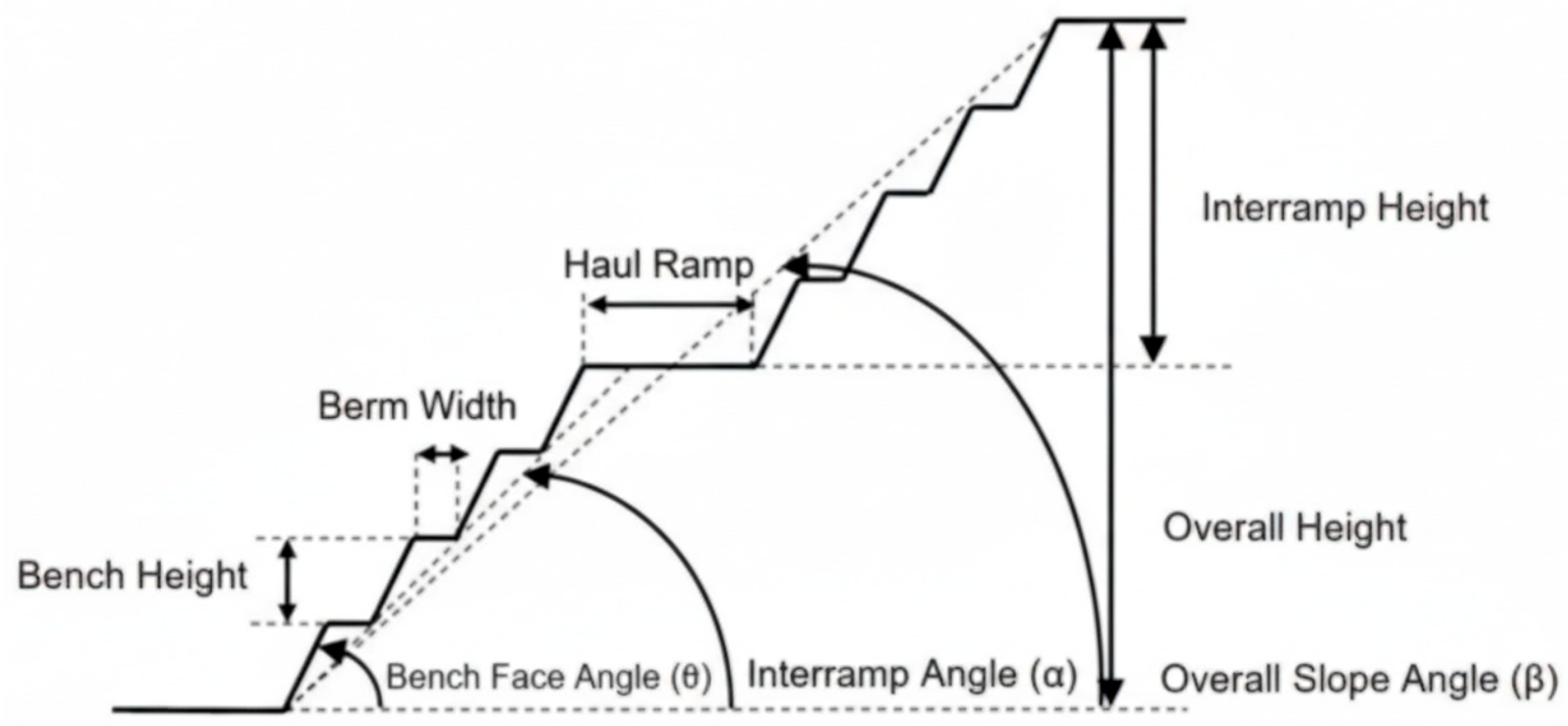
The stability of any slope depends heavily on its overall angle. Rock slope failure probability rises when the slope angle is increased [20]. The stability of a slope is greatly influenced by its curvature and height dimensions. Concave slopes with a radius of curvature smaller than the slope height require slope angles between 5 and 10 degrees steeper than typical analysis methods predict. When dealing with convex slopes where the radius of curvature is less than the slope height, the slope angle needs to be 5 to 10 degrees flatter than traditional guidelines suggest [1]. Open-pit mining requires appropriate slope angles because most natural and excavated slopes display either concave or convex shapes, which affect their stability. Figure 2 illustrates the parameters to be considered during the design of an open pit mine. The selection of appropriate values for each parameter is essential to ensure a safe and cost-effective operation.

2.2. Geological Structures

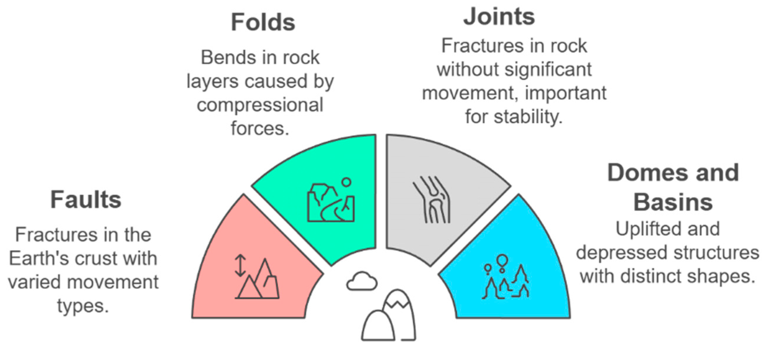
In the rock mass, surfaces with high failure potential are mainly stratification planes and intraformational shear zones, which, like joints and faults, reduce the overall slope stability. Figure 3 is a schematic representation of the different geological structures that can be found in a rock slope. The alignment, continuity, and spacing of these structural elements affect the probability and type of slope failure [1]. The overall stability of the rock mass slope is highly dependent on the dip and dip direction of the geologic structures. Weak planes, such as joints and bedding planes, create conditions for planar or wedge-type slope failure [19].
Planar and wedge-type slope failures are among the most common mechanisms in rock slopes. A planar failure occurs when a discontinuity, such as a bedding plane or joint, is oriented parallel or nearly parallel to the slope face, allowing a block to slide along a single plane. In contrast, wedge failures occur when two or more discontinuities intersect, forming a wedge-shaped block that can slide along the line of intersection. While both failure types are strongly influenced by the orientation, spacing, and persistence of structural features, wedge failures generally involve more complex geometry and multiple planes of movement, making their prediction and mitigation more challenging. Understanding these mechanisms is crucial for selecting the most suitable slope stability analysis methods.

2.3. Groundwater and Hydrogeology

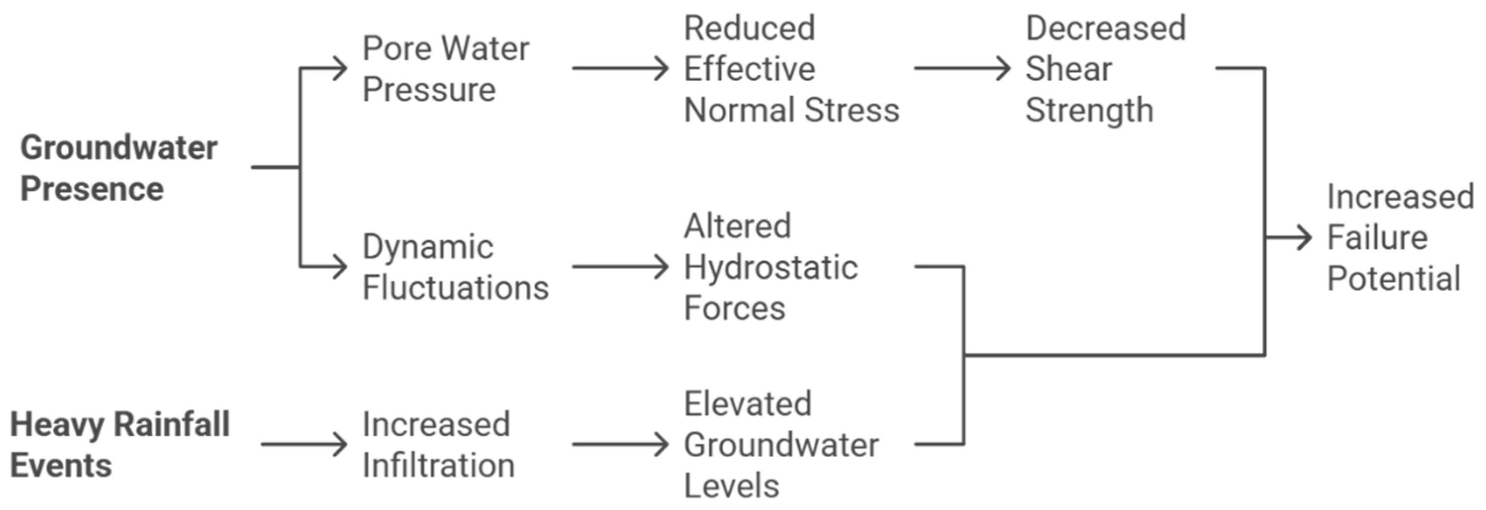
Groundwater presence significantly affects rock slope stability, so monitoring groundwater locations and water table movement must be performed repeatedly. The reduction in effective normal stress in the rock mass by pore water pressure causes both decreased shear strength and elevated chances of slope failure [21]. The intense variation in groundwater levels during heavy rainfall events quickly modifies hydrostatic forces, which leads to unexpected slope collapses [22]. Rainfall can lead to slope instability by promoting water absorption into the ground and elevating groundwater levels. Figure 4 is a flowchart illustrating how groundwater and rainfall can increase the potential for slope failure. In some cases, the analyzed slope shows stability only when dry and becomes unstable when wet conditions occur.
The influence of precipitation on slope stability requires exploration through monitoring systems to assess its impact on stability [23]. Common monitoring methods include the deployment of piezometers and wells to monitor groundwater levels and to install pumping systems to evacuate water, thereby reducing its impact on the rock mass. Inclinometers and automated sensor networks are also used to detect slope displacements and capture real-time hydrological changes. These measurements are critical inputs for slope stability modeling, enabling calibration of hydrogeological parameters such as pore water pressure distribution and permeability. Integrating such monitoring data enables numerical models and Machine Learning algorithms to simulate slope behavior more accurately under varying hydrogeological conditions, thereby improving the reliability of stability predictions and informing proactive slope management strategies.

2.4. Lithology

The mineral composition, alongside the texture and weathering condition of the rock mass, determines the slope’s structural stability and strength. The variation in physical, chemical, and mechanical properties of rock materials results in different failure modes [21]. Slopes become more unstable when weak or weathered rock layers within them create potential failure surfaces. The directional characteristics of rock materials including foliation and bedding planes can result in preferential failure along these structural features.

2.5. Cohesion and Friction Angle

Slope stability critically depends on the shear strength of the rock mass, which is defined by both cohesion and internal friction angle. Increased values of cohesion and internal friction angle result in stronger shear resistance, which enhances slope stability. The potential for slope failures increases substantially when cohesion and the internal friction angle decrease because of weathering processes or water infiltration [24]. Shear strength inadequacy in materials relative to existing shear forces will result in slope failure.

2.6. Blasting and Mining Activities

Rock blasting and excavation of material with production equipment such as electric shovels or excavators can alter the distribution of stresses within the rock mass, which can lead to the appearance of new discontinuities or the reactivation of existing discontinuities and therefore reduce slope stability [1]. Figure 5 illustrates a typical large open-pit operation, where activities such as drilling, loading, and hauling occur simultaneously. All rock blasting generates seismic waves, including P-waves (primary or compressional waves) and S-waves (secondary or shear waves). These waves propagate through the rock mass and can cause vibrations in the surrounding rock up to a distance determined by the weight of the explosive charge used in the blasting design and the properties of the rock mass, as these waves tend to propagate more efficiently in highly fractured rock. Vibrations may destabilize high-steep slopes by triggering microcracks or accelerating displacements, especially during the later stages of open-pit mining when slopes are more exposed and susceptible to failures due to cumulative stress and strain [25]. High-steep slopes are particularly vulnerable due to their geometry, which increases the potential for sliding under dynamic loading conditions.

3. Traditional Deterministic Methods for Slope Stability Analysis

Geotechnical engineering relies heavily on slope stability analysis, which is an essential part of daily mining operation tasks. The analysis needs to predict slope failures to prevent them because such failures create numerous operational problems that mainly affect personnel safety. The deterministic method remains a recognized analysis approach that continues to be widely used today through traditional applications. Deterministic methods use constant input parameter values to determine the Factor of Safety (FOS), which indicates slope stability. In addition, these methods are helpful in the early stages of analysis because they are easily accessible and quick to calculate [26]. On the other hand, they have limitations in modeling the uncertainties and complexity inherent in the rock mass. The following sections detail several deterministic approaches used in slope stability assessment.

3.1. Limit Equilibrium Method (LEM)

Limit Equilibrium Methods are among the most widely used deterministic approaches for slope stability analysis. These methods involve dividing the slope into slices and analyzing the equilibrium of forces and moments acting on each slice [27]. The Factor of Safety is calculated by comparing resisting and driving forces.
F O S = R e s i s t i n g   F o r c e s D r i v i n g   F o r c e s = S h e a r   S t r e n g t h S h e a r   S t r e s s ,
Alternatively, in terms of moments:
F O S =   R e s i s t i n g   M o m e n t D r i v i n g   M o m e n t ,
A FOS > 1 indicates a stable slope, while a FOS < 1 suggests potential failure.
Standard LEM techniques include the Bishop’s Simplified Method, Janbu’s Method, and the Spencer Method. These methods assume a potential slip surface and calculate the Factor of Safety based on the balance of forces along this surface.

3.1.1. Bishop’s Simplified Method

This method assumes circular slip surfaces and simplifies the moment equilibrium equations to make the calculations more manageable. It is beneficial for homogeneous slopes and balances accuracy and computational efficiency well.
F O S = ( c b + ( W u b ) tan ϕ ) ( W   sin α ) ,
where
c = Effective cohesion (kPa)
ϕ = Effective internal friction angle (°)
b = Width of each slice (m)
W = Weight of each slice (kN)
u = Pore water pressure (kPa)
α = Slope inclination (°)

3.1.2. Janbu’s Method

Unlike Bishop’s method, Janbu’s can handle non-circular slip surfaces, making it suitable for more complex slope geometries. It calculates the Factor of Safety using both force and moment equilibrium equations.
F O S = ( c b + ( W u b ) tan ϕ ) F x   ( W   sin α ) ,
where
F x = Correction factor accounting for interslice forces
Janbu’s method is better suited for layered soils and complex slope geometries.

3.1.3. Spencer Method

This method provides a rigorous solution by satisfying each slice’s force and moment equilibrium. It applies to circular and non-circular slip surfaces and is often used in complex slope stability problems [28].
The normal force N is related to the weight of the slice and the interslice forces. It is computed using force equilibrium equations:
N =   W cos α   E l +   E r cos θ ,
where
W = Weight of the slice
α = Base inclination angle of the slice
E l ,   E r = Interslice forces acting on the left and right sides of the slice
θ = Inclination of the resultant force acting at the base
Solving for N and incorporating it into the shear strength equation provides the Factor of Safety (FOS):
F O S   =   ( N tan ϕ + c b ) ( W sin α ) ,

3.2. Finite Element Methods (FEM)

Numerical simulation techniques, such as the Finite Element Method, provide a more comprehensive approach to slope stability analysis. FEM models the slope as a continuum, allowing for the study of complex geometries, material properties, and boundary conditions. Unlike LEMs, FEM does not assume a specific slip surface; instead, it allows for the development of failure surfaces based on the stress–strain behavior of the rock. This provides a more realistic representation of the slope’s performance, particularly for cases with heterogeneous rock conditions or complex loading scenarios [1].
The slope behavior is analyzed by solving the governing equations based on the principles of continuum mechanics:
1.
Equilibrium Equations (force balance)
The general equilibrium equation in FEM for a solid domain under static conditions is:
σ + f = 0 ,
where
σ   = Stress tensor ( σ x x , σ y y ,   σ z z )
f   = Body force vector (e.g., gravity load per unit volume)
In matrix form for a 2D plane strain condition:
σ x x x + σ x y y + f x σ y y y + σ x y x + f y   = 0 0 ,
These equations ensure that forces within the slope are balanced.
2.
Constitutive Equations (stress–strain relationships)
FEM applies constitutive models to relate stresses σ and strains ε using Hooke’s Law for an elastic material:
σ = D ε ,
where
D = Elasticity matrix (depends on Young’s modulus E and Poisson’s ratio ν)
ε = Strain vector
For an elastic-perfectly plastic material, the Mohr-Coulomb failure criterion is commonly used:
τ = c + σ t a n ϕ ,
where
τ = Shear stress
c = Effective cohesion
σ = Normal stress
ϕ = Effective friction angle
3.
Compatibility Equations (deformation continuity)
Strains are related to displacements using:
ε = u ,
where
u = Displacement vector
= Gradient operator
FEM solves displacements first, then derives strains and stresses.
4.
Finite Element Formulation
Using the Principle of Virtual Work, the equilibrium equation is converted into its weak form:
V δ ε T σ d V =   V δ u T f d V + S δ u T t d S ,
where
V = Volume of the slope
S = Boundary surface
δ u = Virtual displacement
t = Traction forces
This equation is discretized into a system of algebraic equations:
K u = F ,
where
K = Global stiffness matrix (assembled from element stiffness matrices)
u = Displacement vector at nodes
F = External force vector (gravity, pore pressure, etc.)
This system is solved numerically using methods like Gaussian elimination or iterative solvers.
5.
Shear Strength Reduction (SSR) Method
A Factor of Safety (FOS) is computed in FEM using the Shear Strength Reduction (SSR) method, where the soil’s shear strength parameters c   a n d     ϕ are progressively reduced until failure occurs.
F O S = c c r = tan ϕ tan ϕ r ,
where
c r ,   ϕ r = Reduced cohesion and friction angle at failure
Failure is indicated when large deformations or non-convergence occur in the FEM solution.
The advantages of FEM include the ability to model complex geometries, nonlinear material behavior, seepage effects, and dynamic loading [29]. On the other hand, the limitations of FEM include the need for more detailed data input, increased computational requirements, and the potential for instability and convergence issues.

3.3. Analytical Methods

Other analytical techniques, such as the limit and vector sum methods, have also been employed for slope stability analysis [20].
The Limit Analysis Method uses optimization techniques to determine the critical slip surface and the Factor of Safety. It provides a rigorous upper and lower-bound solution to the stability problem. On the other hand, the Vector Sum Method calculates the safety factor by considering the equilibrium of forces and moments acting on the potential failure surface [26]. These methods can be helpful in specific situations but are not as widely used as the LEM and FEM techniques.
Infinite Slope Model
This method assumes an infinitely long slope with a failure surface parallel to the ground. It is used for analyzing shallow landslides and only applies to highly weathered or fractured rocks that behave like soil. This approach is unsuitable for blocky, jointed, or intact rock masses.
F O S = c + ( γ h γ w h w ) cos 2 β tan ϕ γ h sin β cos β ,
where
c = Effective cohesion
ϕ = Effective internal friction angle
γ = Unit weight of rock/soil
h = Total rock/soil depth above failure surface
γ w = Unit weight of water
h w = Depth of water table
β = Slope angle
Culmann’s Method
Failure occurs along a single planar surface and can apply to rock slopes with a weak bedding plane or fault. However, it is unsuitable for wedge, toppling, or circular failures.
F O S = c L + W cos β tan ϕ W sin β ,
where
L = Length of plane failure
W = Weight of failing soil mass
Fellenius’ Wedge Method
Failure occurs along a specific failure plane, applicable to planar failures in jointed rock masses. It is not suitable for complex discontinuities or multiple joint intersections.
F O S = c A + N tan ϕ W sin α ,
where
A = Area of the failure surface
N = Normal force on the plane failure
α = Failure plane angle

3.4. Challenges of Deterministic Methods

Deterministic methods are still widely used in slope stability analysis, yet they have several known limitations. Geotechnical parameters such as rock strength, pore water pressure, and slope geometry continue to present fundamental unpredictability as the main challenge [8]. In addition, it depends on fixed single-point values for analysis parameters, which often fail to represent the system’s inherent variability and random behaviors.
Deterministic methods struggle to represent the intricate nonlinear behavior exhibited by soil and rock masses. LEMs rely on simplified assumptions and rigid-body idealization, which fail to represent the complex stress–strain relationships and failure mechanisms found in natural slopes [1]. Advanced numerical approaches, such as the Finite Element Method (FEM) and Finite Difference Method (FDM), are better suited to capture nonlinear stress–strain behavior by incorporating constitutive models of soil and rock. More recently, data-driven approaches, including Machine Learning models, have also shown promise in representing nonlinear interactions when trained on sufficiently large and representative datasets, although their reliability still depends on careful validation against field observations.
They also face difficulties in representing system-wide effects and the interactions that occur between potential failure surfaces within a slope [30].

4. Stochastic Methods for Slope Stability Analysis

Geotechnical engineers have focused on developing stochastic techniques for evaluating slope stability to overcome the constraints imposed by deterministic methods. Stochastic methods, for the most part, arise from the unpredictable nature of the geotechnical properties of the rock mass and the environmental conditions to which the slope may be subjected [3]. Probabilistic methods establish a framework to forecast slope failures and deliver insights on slope stability, reliability, and risk assessment [26].

4.1. Stochastic Finite Element Method (SFEM)

This method proves to be a strong approach for analyzing slope stability, especially when faced with non-normal distributions of geotechnical parameters. The technique applies a first-order approximation at failure point conditions for random variables to establish uniform failure probability measurement across various performance function structures. SFEM excels in its ability to perform reliability analysis on non-normal distributions, which is common in the various geotechnical parameters, and matches the accuracy of the results of one of the most common simulations, which is the Monte Carlo simulation.

4.2. Stochastic Response Surface Method (SRSM)

This approach addresses non-convergence problems found in slope reliability analysis and also performs exceptionally well in solving problems with high nonlinearity [31]. To handle multicollinearity among explanatory variables, researchers have developed variants of SRSM, including Lasso-based methods as well as ridge regression-based algorithms, elastic net regression-based techniques, and stepwise regression-based procedures [32]. The stepwise regression-based SRSM stands out because of its precise and efficient performance in dealing with uncertainties in slope stability.

4.3. Stochastic Simulation with Transition Probabilities and Markov Chains

The approach uses a reliability analysis through transition probabilities and Markov chains to model progressive slope failure across a set timeframe [33]. The method tracks failure spread along essential slip planes using transition probability matrices to determine likelihoods. This approach combines geotechnical uncertainty into stability computations through the use of elastoplastic finite element models to give engineers an essential detailed view of slope failure dynamics [34].

4.4. Jointly Distributed Random Variables (JDRV) Method

The JDRV method functions in probabilistic slope analysis to evaluate the reliability between different limit equilibrium methods. The model applies a truncated normal probability distribution to represent stochastic parameters including soil’s shearing resistance angle, cohesion intercept, and unit weight. Particle swarm optimization evaluates the reliability indices of limit equilibrium methods including Bishop and Janbu methods and reveals different failure probabilities under various conditions.

4.5. Stochastic Kinematic Analysis

Stochastic kinematic analysis provides failure angle estimates for rock slopes when discontinuity data is insufficient. The method relies on algorithms such as Monte Carlo simulation, Latin hypercube sampling and Bayesian estimation techniques to investigate plane and wedge failure mode angles [35]. The method delivers a more objective evaluation compared to empirical techniques by thoroughly addressing the random distribution of discontinuities.

4.6. Challenges of Stochastic Methods

Although stochastic methods provide powerful approaches to manage the uncertainty of geotechnical rock mass parameters, they face significant difficulties because they require large computational resources and much time when applied to large three-dimensional slope models [3]. The process of accurately defining the probabilistic distributions for geotechnical parameters continues to be problematic due to limited access to field data [36].
The practical implementation of stochastic methods within engineering workflows presents significant difficulty because geotechnical engineers often lack access to necessary specialized software and expertise [36]. The enhancement of computational capabilities together with growing data accessibility will drive the increased implementation of stochastic methods in slope stability analysis which will deliver more dependable and thorough evaluations of slope stability.

5. Machine Learning Methods

Machine Learning (ML) techniques have become essential tools in a wide range of problems in different fields, from engineering to medical sciences, in recent years. With their fast and exponential development, many ML algorithms have been developed and applied in various areas of geotechnical engineering. In this regard, their ability to perform slope stability analysis has recently attracted a great amount of attention to assess the performance of ML models for slope failure prediction [26].
The ability of ML methods to find out the complex and nonlinear relations among geotechnical parameters affecting the stability of slopes is one of the advantages of these methods. Moreover, it is possible to apply advanced ML models that can handle data from different sources, such as field measurements or real-time measurements like radar data, and take all the information of the site into account in the analysis. On the other hand, one of the most appealing aspects of ML is its ability to quickly work with large datasets and figure out the most effective factors in the results of slope failure predictions. In this way, not only will the reliability of the models increase, but practitioners will also be able to check the input parameters and modify the database.
The most widely adopted machine-learning methods for mining slope stability prediction include Random Forests, Support Vector Machines, and Gradient-Boosting Machines because of their exceptional accuracy and robust performance. Decision Trees and k-nearest Neighbors see less frequent use because they offer simplicity and interpretability [37]. Advanced ensemble hybrid models that combine multiple algorithms are becoming increasingly popular because they improve prediction accuracy. Machine-learning techniques fall under the Supervised and Unsupervised learning categories depending on the availability of labeled data, such as stable or unstable slopes.

5.1. Supervised Learning

Supervised learning models are trained on historical slope stability data, where the input variables (e.g., slope geometry, soil/rock properties, and groundwater conditions) are paired with the corresponding slope stability outcomes (stable or unstable). Based on their characteristics, these models can then predict the stability of new slopes. Supervised learning has been applied in geotechnical engineering to classify slopes as stable or unstable and estimate the Factor of Safety or probability of failure. For example, the Gradient Boosting Machine has shown excellent performance in predicting circular mode failures in slope stability analysis [38].
Commonly employed supervised learning algorithms in slope stability analysis include:

5.1.1. Decision Trees (DT)

Machine learning utilizes decision trees as basic yet effective instruments for data-driven decision-making. The approach works by dividing complex issues into multiple smaller questions derived from different features within the dataset. Each step in the decision tree splits data using one variable to create branches, which leads to different outcomes. The process continues and moves on to further branches until it stops at a decision point or terminal prediction. The ease with which the results are developed and subsequently interpreted makes this model very popular for applications that require transparency, knowing how the algorithm is developed before delivering the prediction and presenting it to a team to make a joint decision. Decision trees enable engineers to assess the relative importance of input variables because they generate results that people can easily interpret. Figure 6 illustrates a typical flowchart for the DT methodology. In this case, it analyzes the stability of a slope with certain parameters that have been developed. Decision trees demonstrate sensitivity to minor modifications in training data and exhibit tendencies to both overfit and maintain high variance levels. Decision trees enable engineers to forecast various slope failure types while helping them determine whether slopes are stable or unstable.

5.1.2. Random Forest (RF)

The Random Forest (RF) algorithm stands as a powerful machine-learning technique useful for slope stability predictions. This method proves exceptionally effective as it handles complex datasets while providing superior predictive accuracy [10]. The Random Forest algorithm works as an ensemble learning method by creating several decision trees during training and then outputs the most common prediction from these trees when classifying data points [10]. The RF algorithm stands out for its robustness and ability to handle large-scale datasets that contain numerous input variables. Slope stability evaluations benefit from this method because they are complex systems affected by multiple stability-determining factors.
Geotechnical engineers use the Random Forest algorithm to evaluate slope stability. The model utilizes multiple geotechnical parameters, including unit weight, cohesion, internal friction angle, slope angle, slope height, and pore water pressure coefficient as input features [39]. The computational approach establishes an intricate nonlinear correlation between multiple variables and slope stability status, which enables precise predictive outcomes.
This model is very accurate for slope analysis. For example, in the research conducted by Moayedi et al., the stability of a slope was evaluated by estimating the Factor of Safety using several ML models, where the RF model stood out over the others with a predictive accuracy rate of 0.98 [40]. The model’s dependability and precision in stability forecasting are established through regular assessments using metrics like AUC, accuracy, and confusion matrices [41]. One major advantage of using Random Forest is its ability to highlight which features impact slope stability. Research shows that cohesion stands out as the critical factor having a major impact on predictions of stability [40].

5.1.3. Support Vector Machine (SVM)

The Support Vector Machine (SVM) is a sophisticated supervised Machine Learning method widely used for predicting slope stability [40]. This supervised learning algorithm establishes an optimal hyperplane in a high-dimensional space, effectively dividing the data into distinct categories while maximizing the margin between them. It is a robust ML approach used for both classification and regression tasks, and it has shown effectiveness in predicting slope stability. Additionally, the SVM framework is particularly well-suited for this analysis due to its ability to handle complex, nonlinear relationships between input variables and the stability conditions of slopes [42]. In slope stability assessment, SVM models are systematically trained to use geotechnical parameters, including soil characteristics, slope configurations, environmental influences, and recorded slope stability results [40].
Various studies have used SVM to predict slope stability by analyzing slopes’ geotechnical and geometric properties. For instance, one study employed SVM to classify slope stability status, achieving an accuracy of 100% by using structural risk minimization principles to minimize generalization error rather than just training error [43]. Another study combined SVM with particle swarm optimization (PSO) to enhance parameter selection, resulting in improved forecasting accuracy for slope stability [44].
Hybrid models have also shown great success with the integration of SVM and optimization approaches to effectively predict slope stability. For example, a hybrid method consisting of least squares support vector machine (LSSVM) and Particle Swarm Optimization (PSO) was able to effectively predict slope stability by updating the LSSVM parameters [45]. In addition, an improved SVM was trained using the grid search and cross-validation method to predict the Factor of Safety of slopes and outperformed other ML methods [46]. One of the benefits of SVMs is that they are known to be efficient with small datasets. This is another major intersection with slope stability as data from field conditions may be sparse. In addition, SVM models have the ability to provide probabilistic output, which can be used to make risk-based decisions in the mining industry.

5.1.4. Gradient Boosting Machine (GBM)/XGBoost

Gradient Boosting is a supervised learning technique designed to improve predictive accuracy by sequentially combining multiple weak learners, typically decision trees, into a strong ensemble model [38]. Each new tree is built to correct the residual errors of the previous ones, gradually improving the model’s performance. This iterative correction process is what gives gradient boosting its robustness and high predictive capability.
Two of the most widely used implementations of this approach are the Gradient Boosting Machine (GBM) and eXtreme Gradient Boosting (XGBoost). GBM introduced the basic framework, offering solid performance in both regression and classification tasks. XGBoost refined this concept by introducing parallel processing, regularization terms (L1 and L2) to mitigate overfitting, and efficient handling of missing data, which made it computationally faster and more generalizable [42].
Common hyperparameters in GBM and XGBoost include the number of estimators (trees), learning rate, maximum tree depth, and subsampling rate. The learning rate controls the contribution of each tree, while maximum depth defines model complexity. Careful tuning of these hyperparameters is essential to balance model bias and variance.
In the context of geotechnical and slope stability analysis, GBM and XGBoost are particularly suited due to their ability to model complex nonlinear relationships, account for parameter interactions (e.g., between shear strength, slope geometry, and groundwater conditions), and handle noisy or incomplete field data. Their capability to rank input feature importance also helps identify the most influential geotechnical parameters governing slope behavior.
Compared to simpler algorithms like Linear Regression or Support Vector Machines, GBM and XGBoost provide superior flexibility in capturing nonlinear patterns without requiring prior assumptions about data distribution. However, they may require more computational resources and careful hyperparameter optimization to avoid overfitting, especially when dealing with small or unbalanced datasets.

5.1.5. Artificial Neural Networks (ANNs)

Artificial Neural Networks (ANN) have been used in different areas of Machine Learning, and the concept is derived from a computer model that mimics the functions of the human brain [26]. The networks work based on several artificial neurons that collectively perform simple information-processing functions of neurons present in a biological brain. The most salient application of ANNs is pattern recognition within a dataset. The efficiency of this model in handling and solving complex nonlinear relationships makes it suitable for handling nonlinear problems such as slope stability problems [40].
ANNs perform slope prediction by being trained on a set of data where a range of geotechnical parameters such as soil and/or rock properties, slope geometry, and historical slope failures are fitted and fed into the model. The model learns the relationship that each parameter has on slope behavior to make a reliable prediction of the Factor of Safety (FOS) of a slope.
The structure of a typical ANN model for slope behavior is a multilayer network that consists of an input layer, one or more hidden layers, and an output layer. The input layer of a typical ANN model for slope analysis will take in the variables such as slope geometry, geotechnical parameters, and hydrological conditions as the inputs. The model is trained to use data from the historical record by continually updating the internal weights of the network. The ANN model learns the relationship between the input conditions and the corresponding Factor of Safety (FOS) as the output. The model is then validated by comparing its predicted value of FOS to the actual measured FOS. The statistical performance of the ANN model is usually based on the correlation coefficient (R) which shows the goodness of fit between the model and the validation data. The Root Mean Square Error (RMSE) also shows the difference between the model predictions and the actual measured values. The results are then used to make informed decisions on the future performance of a slope.
ANNs are also suitable to describe the failure mechanisms in some cases. Three-dimensional (3D) realizations have been implemented by several researchers, which have become very important in mine slopes. This is because open pit mines and waste dumps are large slopes with curved benches and levels that cut across one another. In such slopes, failure mechanisms may be initiated and developed that are not considered during regular two-dimensional (2D) slope stability assessments. A joint set that is not considered a potential failure plane in 2D may form a critical failure plane in 3D. The 3D ANN model accounts for spatial aspects of geometry and geology that are not accounted for in 2D models, which provides more realistic slope performance predictions. This has been implemented using hybrid models by coupling genetic algorithms with ANN for slope stability predictions.

5.1.6. Key Advantages of Supervised Learning

  • High Prediction Accuracy: The supervised learning algorithms random forest (RF), support vector machine (SVM), and extreme gradient boosting (XGBoost) demonstrate exceptional accuracy when predicting slope stability results.
  • Interpretability: Through supervised algorithms stakeholders can understand which input variables most affect slope stability because these algorithms reveal their relative importance.
  • Handling Complex Data: Advanced modeling systems have the capacity to evaluate numerous determinants like slope angle while also considering vegetation cover and structural conditions. The system allows comprehensive stability analysis while enabling detailed studies of slope behavior.
  • Improved Computational Efficiency: Supervised learning models within Machine Learning frameworks function as surrogate models that enhance computational efficiency when analyzing stochastic slope stability. The resulting effect is a reduction in costs traditionally incurred by deterministic methods.
  • Robustness and Reliability: Ensemble-based supervised learning frameworks such as RF and XGBoost demonstrate significant robustness for classification tasks by providing reliable predictions across multiple datasets and environmental conditions.
  • Feature Importance Analysis: Supervised learning approaches can be adjusted and refined for different datasets and environmental conditions which makes them effective tools for slope stability analysis in multiple geographic and ecological areas.

5.2. Unsupervised Learning

Slope stability analysis now sees unsupervised learning algorithms as highly robust methods. Data-focused methods enable identification of hidden patterns and clusters together with anomalies in geotechnical datasets which provide essential understanding of complex interactions that determine slope behavior [47].
Unsupervised algorithms focus on finding patterns and similarities in the data without relying on pre-assigned labels or labels entered in conjunction with the data to be analyzed, according to researchers these methods can work in conjunction with supervised learning approaches to improve the performance of prediction systems [48]. Such methods generate significant insight into the inherent configuration of the dataset and the connections between data elements that help uncover essential factors affecting slope stability.

5.2.1. K-Means Clustering

K-means clustering is a popular unsupervised learning technique that groups data into a predefined number of clusters (K) based on the similarity of their features [49]. In slope stability analysis, this method is used to identify clusters of slopes that share similar geotechnical and environmental characteristics. Engineers can use the variable stability conditions reflected in these clusters to improve their understanding and classification of slope behaviors throughout a project site. Slopes possessing equivalent rock strength and slope angle, along with comparable groundwater effects, can naturally form the same cluster, which exposes patterns that raw data does not show at first glance [3].
K-means clustering has been used to enhance the Slope Mass Rating (SMR) system for slope stability analysis. Integrating K-means with fuzzy c-means clustering improves the SMR system’s classification results by reducing subjective judgments and providing more reliable slope stability assessments. This approach allows for a more objective classification of slopes based on continuous and discrete functions, increasing the reliability of the SMR system.
The Adaptive K-means Clustering-Based RSSs (AKCBR) method has been developed to improve the efficiency of slope reliability analysis. This method adaptively selects representative slip surfaces (RSSs) from potential slip surfaces (PSSs), offering a statistically sound approach that is less sensitive to variations in soil properties. AKCBR is more efficient and yields comparable reliability results to an existing method [50].

5.2.2. Gaussian Mixture Models (GMM)

Gaussian Mixture Models (GMM) are a robust statistical framework for describing complex probability distributions by combining multiple Gaussian distributions. Unlike K-means clustering, GMMs can capture nonlinear dependencies and intricate distributions within the dataset by treating it as a mixture of Gaussian distributions [29]. Studies suggest that GMMs perform better than K-means in some slope stability applications because they are more capable of handling the inherent uncertainties and nonlinearities in the data. While GMMs offer a more sophisticated method, they also require more computational resources and careful parameter optimization. Additionally, this approach uses prior knowledge about the dataset, which may not always be available in slope stability scenarios. GMMs can be particularly useful for applications with well-defined data properties.
This method proves especially useful when addressing the nonlinear connections and inherent uncertainties present in geological systems. In a rock slope with alternating competent and weathered layers, it becomes difficult to distinguish each layer’s effect on total stability. The model identifies transitional stability states between rock layers that more rigid classification systems fail to detect because it considers overlapping patterns [51].
The primary advantage of the method is its capability to handle complex distributions, even though it needs precise parameter tuning and some basic understanding of data structure. The algorithm operates efficiently despite its higher computational demands because the Expectation-Maximization (EM) algorithm enables fast convergence while maintaining accuracy [51].
Gaussian Mixture Models provide a resilient framework for analyzing slope stability. They effectively handle the complex and variable nature of geological environments. Their ability to model diverse distributions and the computational efficiency of parameter estimation make them valuable tools in this field.

5.2.3. DBSCAN (Density-Based Clustering)

The Density-Based Spatial Clustering of Applications with Noise (DBSCAN) algorithm is widely recognized across various scientific fields for its ability to handle noise and identify clusters of different shapes without needing prior knowledge of the number of clusters [52]. In slope stability assessment, DBSCAN offers an innovative method for segmenting discontinuities in geological formations, which is essential for accurate modeling and analysis.
DBSCAN categorizes discontinuities in geological structures, which is vital for creating a three-dimensional network model that includes random discontinuities [53]. This approach reduces the limitations of traditional graphical analyses, which are often subjective. DBSCAN eliminates the need to pre-define cluster centers, and the effective removal of outliers improves the accuracy of the results. This method has been successfully applied to real-world datasets, such as discontinuity orientation data from the Maji dam site, showing good agreement with field measurements.
Unlike traditional techniques like the fuzzy C-means clustering algorithm, DBSCAN offers better accuracy by removing outliers and not requiring predefined cluster centers. As a result, it is a more advantageous option for general analyses of rock mass discontinuities [54].
DBSCAN can also identify spatial patterns within slope stability datasets, such as grouping failed slopes with similar characteristics. These insights can significantly improve the understanding of the fundamental factors contributing to slope failures and help in developing more targeted slope management strategies.
Despite its advantages, DBSCAN has limitations. These include performance issues with large datasets, difficulty identifying clusters with varying densities, and dependence on user-defined parameters [55].

5.2.4. Key Advantages of Unsupervised Learning

Unsupervised Machine Learning provides multiple benefits when assessing slope stability. The ability to process massive datasets without the necessity of labeled data represents significant benefits within geotechnical engineering because labeling such data requires extensive time and high costs.
The application of these techniques exposes concealed patterns and relationships within data that may not be easily recognized through standard analytical methods. By augmenting automation in data analysis and decision-making processes these methods can lead to improved efficiency and consistency in evaluating slope stability.
  • Data Handling and Preprocessing: Efficient management and preprocessing of large datasets by unsupervised learning is an important component in slope stability analysis due to the need to integrate and standardize data collected from various sources, such as laboratory test results, geotechnical measurement equipment, and radars [9].
  • Pattern Recognition: By identifying data patterns and anomalies, it enables detection of potential slope failure by analyzing geotechnical and environmental factors without the need for prior data labeling [56].
  • Dimensionality Reduction: The use of clustering and principal component analysis (PCA) reduces data complexity which improves both the visualization and interpretation of slope stability variables [9].
  • Anomaly Detection: Outlier identification and unusual pattern recognition in slope data through unsupervised methods provide indicators of potential instability and failure risks [56].
  • Adaptability: Unsupervised learning adjusts to new conditions and data inputs, making it ideal for dynamic slope monitoring and analysis applications [57].
Unsupervised learning methods add value to slope stability analysis which surpasses traditional supervised approaches, yet they present substantial difficulties including model interpretation and algorithm parameter selection.
It is essential to evaluate the performance and suitability of Machine Learning techniques by estimating their accuracy particularly when dealing with classification problems. Researchers must choose the best evaluation metrics like accuracy, precision, recall, F1-score, or AUC-ROC based on their research goals while considering available information and the potential costs of various error types.
Accuracy is defined as:
A c c u r a c y   =   N u m b e r   o f   C o r r e c t   P r e d i c t i o n s T o t a l   N u m b e r   o f   P r e d i c t i o n s
  • Or, in terms of a confusion matrix:
A c c u r a c y = ( T P + T N ) ( T P + T N + F P + F N )
where
TP (True Positives): Correctly classified positive instances
TN (True Negatives): Correctly classified negative instances
FP (False Positives): Incorrectly classified negative instances as positive
FN (False Negatives): Incorrectly classified positive instances as negative
The accuracy metric works well when there is an equal distribution between positive and negative instances in the data. Computing this metric requires little effort but it does not always serve as the optimal evaluation standard. A train-test split, or cross-validation process should be used to achieve reliable accuracy estimation.
When dealing with imbalanced classes, accuracy produces an exaggerated impression of the model’s effectiveness. A model achieves 95% accuracy by labeling all examples as unfavorable in a dataset where 95% of the instances are harmful but fail to learn anything useful. Other metrics must be used to address this issue.
  • Precision: Focuses on the accuracy of positive predictions. It is crucial when false positives are costly (e.g., spam detection).
  • Recall: Measures the model’s ability to find all actual positive instances. It is crucial when false negatives are critical (e.g., medical diagnosis).
  • F1-score: The harmonic mean of precision and recall, providing a balanced measure.
  • AUC-ROC: Summarizes the model’s performance across different classification thresholds.

5.2.5. Comparative Analysis of Supervised and Unsupervised Learning

Supervised and unsupervised learning paradigms serve different purposes in slope stability analysis. Supervised learning relies on labeled datasets, where input parameters (e.g., slope geometry, geotechnical properties, hydrological conditions) are paired with known outputs such as slope stability classifications or Factor of Safety values. This enables direct prediction and classification, making supervised methods ideal for hazard assessment when sufficient historical failure data exist. Typical supervised techniques include Decision Trees, Support Vector Machines, and Random Forests, which require well-curated training data and benefit from feature selection for improved interpretability. In contrast, unsupervised learning operates without labeled outputs, instead seeking to identify inherent structures or patterns within the data.
This approach is useful for exploratory analysis, anomaly detection, clustering slope conditions, and identifying latent factors influencing stability, particularly when labeled datasets are limited. Common unsupervised methods include Clustering algorithms and Gaussian Mixture Models. While unsupervised learning is less dependent on prior knowledge, it often requires careful interpretation by experts to translate patterns into actionable insights. Understanding the strengths and limitations of each paradigm is essential for selecting the most suitable approach based on the available data and engineering objectives.

6. Analysis and Discussion

Recognizing the most advantageous method among the various forecasting techniques in this review presents a significant challenge. Many methodologies lack sufficient applications for a thorough evaluation, and these applications rarely involve predictions made before an event occurs. Additionally, few scholarly articles have directly compared different methodologies.
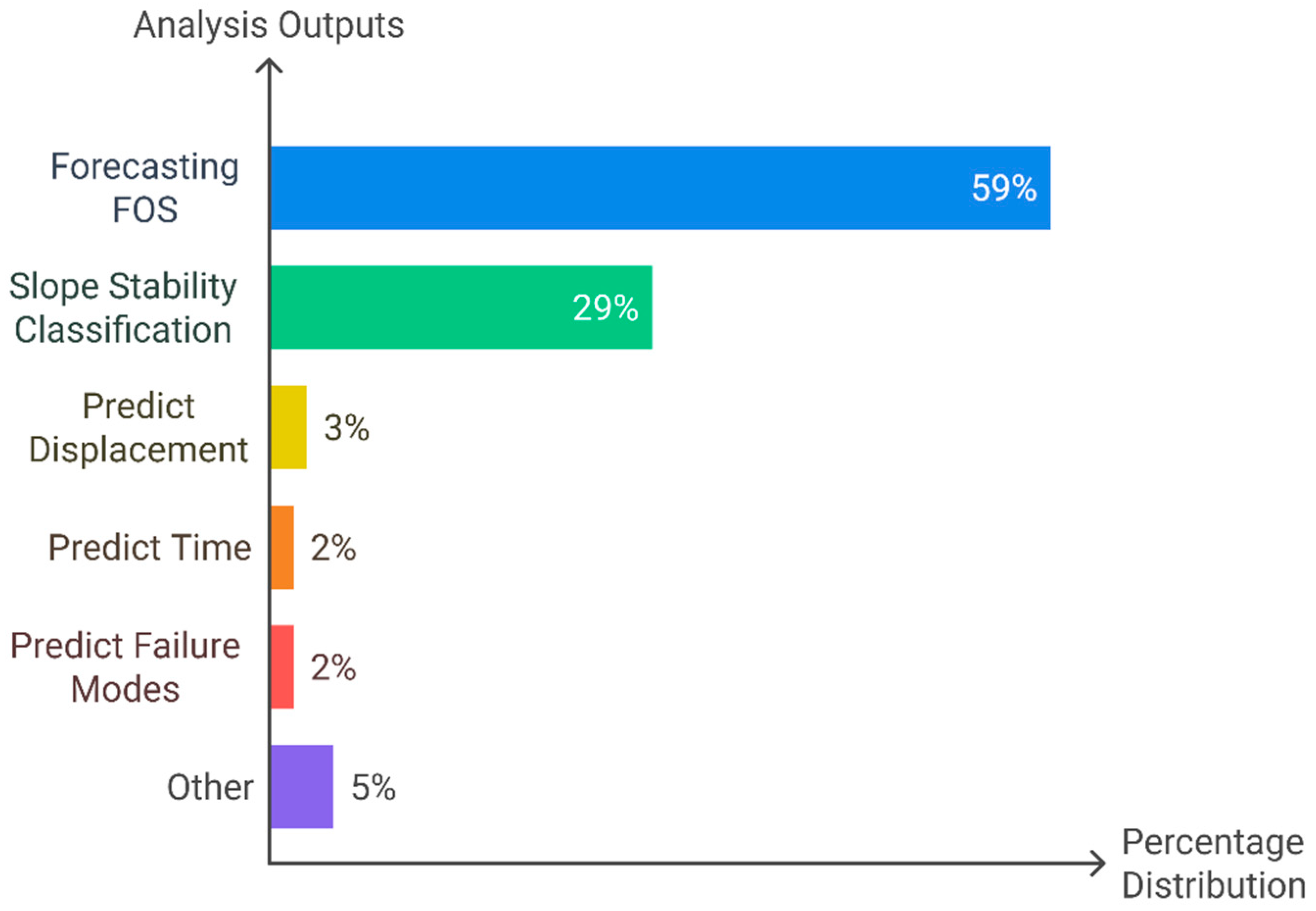
This manuscript analyzed 54 papers focused on slope stability analysis and classified them according to their output goal for each one. Consequently, this review stated that slope stability studies primarily focus on predicting the Factor of Safety (FOS), making it the most common approach. Slope stability classification is also widely used, while predictive methods for displacement, failure time, and failure modes are less common. Figure 7 illustrates the primary research outputs analyzed in this literature review. It is evident that research focused on the forecasting of FOS constitutes the majority, accounting for 59% of the 54 papers analyzed. This trend suggests a focus on overall stability and safety rather than specific failure mechanisms, likely due to the complexity and data requirements of those models.

6.1. Most Effective Machine Learning Techniques to Estimate the Factor of Safety

Machine Learning methods have been increasingly utilized to provide rapid and accurate predictions. After reviewing 32 research studies about the strengths and limitations of various machine-learning approaches to estimate the Factor of Safety (FOS) in slope stability analysis and comparing the performance through the parameters R-squared (R2), Root Mean Square Error (RMSE), and Mean Squared Error (MSE), the three most effective ML methods identified for this purpose are:

6.1.1. Multilayer Perceptron (MLP)

The Multi-Layer Perceptron (MLP) constitutes a sophisticated artificial neural network (ANN) characterized by an arrangement of multiple neuron layers, rendering it exceptionally proficient in discerning intricate, nonlinear correlations within geotechnical datasets. The training process of the MLP is carried out through backpropagation, with optimization achieved through techniques such as Stochastic Gradient Descent (SGD) or the Adam algorithm. MLP can assimilate knowledge directly from geotechnical variables, encompassing soil characteristics and slope configurations. Due to its adeptness in modeling nonlinear associations, the MLP has demonstrated superior efficacy in slope stability forecasting when juxtaposed with conventional techniques.
An investigative endeavor conducted by Nanehkaran et al. [4] utilized data derived from 70 slopes in the South Pars region of southwestern Iran to accurately predict the Factor of Safety (FOS). They compared five ML models: MLP, Support Vector Machines (SVM), k-Nearest Neighbors (k-NN), Decision Trees (DT), and Random Forest (RF). The findings indicated that MLP emerged as the superior model, attaining a Precision of 0.938, an Accuracy of 90%, a Mean Squared Error (MSE) of 0.103, and a Root Mean Square Error (RMSE) of 0.099. Furthermore, it exhibited robust generalization capabilities when evaluated against novel datasets.
Moreover, a research endeavor by Bui et al. [42] implemented an Ensemble MLP model, which integrates multiple MLP networks, to predict the Factor of Safety for slopes in Vietnam, utilizing a dataset comprising 630 samples of a natural slope. The performance of the MLP was juxtaposed with that of Gaussian Process Regression (GPR), Multiple Linear Regression (MLR), Simple Linear Regression (SLR), and Support Vector Regression (SVR), wherein the MLP attained the highest cumulative score of 50 points (R2 = 0.994, RMSE = 0.713, RAE = 0.098), thereby surpassing all other models in terms of precision and operational efficacy.

6.1.2. Support Vector Regression (SVR)

Support Vector Regression (SVR) is a regression-based version of the Support Vector Machine (SVM) algorithm, which is effective at modeling complex, nonlinear relationships and is designed to handle continuous output variables, such as the Factor of Safety. It finds the optimal hyperplane that best fits the training data by minimizing error while maintaining robustness to outliers. Additionally, it can be optimized using kernel functions such as the Radial Basis Function (RBF) and Polynomial kernels.
Lei et al. [46] tested 166 groups of slope cases from different sources in China. They proposed an improved SVR model as the primary prediction tool and used the grid search method with 5-fold cross-validation for hyperparameter optimization. The results show that the model can describe the nonlinear relationship between features and the Factor of Safety. The testing dataset’s R2, MAPE, MAE, and RMSE were 0.901, 7.41%, 0.082, and 0.133, respectively.

6.1.3. Stochastic M5P Model

The M5P model combines decision-tree and linear regression models. It is similar to a standard decision-tree model. However, rather than having a categorical label for every terminal node, it incorporates a linear regression model. When the terminal node is encountered, a multiple linear regression model is performed on the data within the terminal node, rather than fixed predictions as in the case of standard decision-trees. This is useful for increasing prediction accuracy, providing continuous and coherent predictions compared to discrete outcomes.
Nouri et al. [58] investigated the ability of soft-computing-based models, such as Random Forest (RF), Random Tree (RT), M5P, Bagging M5P, and Stochastic M5P, for predicting the Factor of Safety of homogeneous slopes. To this end, the SLOPE/W Geostudio software was used to model a simple homogeneous earthen slope employing the limit equilibrium method (LEM). The data analyzed in the study is synthetic and generated through simulation. The 508 safety factor model values were examined with 344 for training and 164 for testing. The Stochastic M5P model using combined wavelet-PSO approach achieved promising results with a coefficient of correlation (CC) of 0.9950, root mean square error (RMSE) of 0.0716, mean absolute error (MAE) of 0.0522, Scattering Index (SI) of 0.0405 and Nash-Sutcliffe model efficiency coefficient (NS) of 0.9894 during testing stages. These metrics indicate a relatively high accuracy of model’s predictions. The advantages and limitations of three popular ML models used for Factor of Safety prediction are listed in Table 1.

6.2. Most Effective Machine Learning Techniques for Classifying a Slope as Stable or Unstable

Classifying a slope as stable or unstable is critical in geotechnical engineering, influencing decisions related to infrastructure safety, landslide prevention, and risk assessment [59]. Traditional methods such as Limit Equilibrium Methods (LEM), Finite Element Methods (FEM), and Finite Difference Methods (FDM) require extensive computations and are sensitive to parameter variations [14].
To determine the most effective techniques, 16 research papers focusing on classification were reviewed, and the performance of each technique was analyzed using the parameters of Area Under the ROC Curve (AUC) and accuracy. Machine learning (ML) techniques provide a faster, more adaptable, and often more accurate alternative. Among various ML models, the most effective for binary classification of slope stability are:
  • Extreme Gradient Boosting (XGBoost)
  • Random Forest (RF)
  • Support Vector Machines (SVM)
Each model has distinct advantages and is suited for different dataset sizes and complexity levels.

6.2.1. Extreme Gradient Boosting (XGBoost)

XGBoost is an advanced ensemble learning technique based on gradient-boosting decision trees (GBDTs). It builds decision trees sequentially, with each tree correcting errors made by the previous one. XGBoost is optimized for speed and accuracy, making it highly effective in complex classification tasks like slope stability analysis. Additionally, XGBoost is robust against overfitting and can handle missing values and nonlinear relationships [37,38].
Pham et al. [60] developed classification models using ensemble learning to estimate the stability status of slopes. Two main ensemble techniques were used to implement these ensemble classifiers: parallel ensembles with homogeneous and heterogeneous structures, and sequential ensembles. Eight versatile learning algorithms (i.e., KNN, SVM, GP, GNB, QDA, ANN, DT, and SGD) were also used for comparison. The authors analyzed a database of 153 slope cases documented in published literature from different countries between 1930 and 2005. The XGBoost-based classifier (XGB-CM) achieved the highest accuracy with an F1 Score of 0.914, an accuracy of 90.3%, and an AUC (Area Under ROC Curve) of 0.95. Furthermore, XGB-CM correctly identified 16 out of the 16 stable slopes and 12 out of the 15 failure slopes, indicating its excellent performance.

6.2.2. Random Forest (RF)

A random forest is a type of ensemble learning model that builds several decision trees and combines the predictions in order to improve the classification accuracy. The robustness of RF models in the presence of noisy data and feature interactions (i.e., the effect of one fit predictor on the response variable is conditional to the value of another predictor) offers the potential to analyze the complexity encountered in slope stability analysis [61]. Bagging-based models randomly select subsets of data to build multiple trees, reducing variance. However, it is crucial to identify the most influential parameters (e.g., cohesion, slope angle, etc.).
Yang et al. [20] focused on slope stability prediction employing optimization and Machine Learning methods. Their research collected 117 data points from different sources and research studies. The data were split into training and test sets (70/30). They used five ML algorithms that included Support Vector Machine (SVM), Random Forest (RF), Nearest Neighbor (KNN), Decision Tree (DT) and Gradient Boosting Machine (GBM). The model with the highest AUC (0.944) was the RF with a Kolmogorov–Smirnov (KS) cut-off. The proposed model was tested and demonstrated an improved performance over benchmark techniques. Cohesion was found to be the most influential factor on the slope stability, with an influence factor of 0.327, or about one third of the overall influence. Pore water pressure was the least significant factor.

6.2.3. Support Vector Machine (SVM)

SVM is a kernel-based classification model that finds an optimal decision boundary (hyperplane) to separate stable and unstable slopes [20]. It is particularly effective for small datasets and complex, nonlinear relationships. Moreover, it ensures a well-defined boundary between stable and unstable slopes and is less sensitive to noise than decision trees.
Qi & Tang [62] investigated the performance of six integrated artificial intelligence (AI) approaches for slope stability prediction based on metaheuristic and ML algorithms. Six ML algorithms, including logistic regression, decision tree, random forest, gradient boosting machine, support vector machine, and multilayer perceptron neural network, were used for the relationship modeling, and the firefly algorithm (FA) was used for hyperparameter tuning. After considering the slope failure mechanism and geological conditions, they analyzed 148 slope cases to prepare the dataset. The largest area under the curve (AUC) was achieved using the optimum SVM model (0.967) with 0.96 accuracy. Similarly, cohesion was the most influential variable for predicting slope stability, achieving a 0.310 importance score out of 1. Table 2 compares the strengths and weaknesses of three widely used Machine Learning models for slope stability classification.

6.3. Analysis of the Results

The findings presented in this literature review show that advanced Machine Learning methods can accurately predict slope stability. These models can categorize slopes into stable and (un)stable classes with an accuracy of better than 90% in most cases. This represents a significant improvement over traditional methods of slope stability analysis, which typically require the use of complex constitutive models and complex model calibration.
Since hard evidence supporting the superiority of any one technique is lacking, using several methods in parallel is recommended. This approach could provide a more stable and reliable evaluation of slope stability. Moreover, the choice of the optimal method could also depend on the nature of the dataset, intended application, and the degree of interpretability needed. Innovations must also be considered progress in related disciplines such as civil engineering, in which successful methods are currently being used to the same ends, despite some differences in specific parameters, due to site-specific conditions.
In engineering practice, the choice between traditional computational methods and Machine Learning-based assessments depends on the phase of slope stability evaluation. Traditional methods, such as Limit Equilibrium or Finite Element analyses, are most appropriate in the design and planning phases, providing a well-established basis for determining slope geometry, material properties, and safety factors under assumed conditions. Machine Learning approaches, in contrast, are particularly valuable during the operational and monitoring phases, where real-time data from sensors, geotechnical instruments, or remote sensing technologies can be continuously integrated to refine stability predictions. This complementary use allows traditional methods to establish the foundational design parameters, while ML offers adaptive, data-driven updates that improve prediction accuracy, capture evolving slope behavior, and support proactive risk management. Integrating both approaches strategically enhances engineering decision-making throughout the slope lifecycle.
Recent years have seen an emerging trend towards using advanced Machine Learning regression models for the analysis of soil and rock slope stability. This type of analysis is generally more appropriate when accounting for the variability in rock masses and geological conditions at a site. Leveraging these models, which do not require any predefined labels, can potentially make them more effective, but may also bring along more uncertainty. The expertise of geotechnical engineers interpreting the results becomes a crucial factor in presenting recommendations for those working near the slopes. Advancing technology to improve the accuracy and reliance of slope stability analysis is of paramount importance to all facets of mining, particularly given the emphasis on safety.
The ML algorithms presented in this paper have a significant potential for enhancing slope stability analysis by forecasting the Factor of Safety. For example, Multilayer Perceptron, SVM regression, Stochastic M5P are techniques that have shown a promising level of accuracy and computational efficiency for predicting the FOS directly. In addition, as a general guideline, MLP is a good choice for large datasets, while the SVR performs well when nonlinearity needs to be considered in small datasets, and M5P is suitable in cases where a fast and easy-to-understand model that balances accuracy and efficiency is required.
Moreover, binary classifiers such as Support Vector Machine and Gradient Boosting have shown to be efficient in assessing the slope condition, i.e., stable or unstable, without directly computing the FOS. Such a comparison of various methods can be useful in determining the most suitable approach for a particular situation in terms of the size of the dataset, nonlinearity and computational burden.
Further improvement of the robustness and reliability of predictions of slope stability could be obtained by introducing uncertainty analysis methods such as Monte Carlo simulations and Bayesian methods.
Although these innovations are promising, there is a need for more research to assess their capabilities and limitations. By increasing dataset size and diversity, conducting comparative studies across different mining operations and slope conditions, and evaluating ensemble approaches that integrate multiple models, the prediction systems may prove even more robust and reliable. Another advantage could be derived from the use of hybrid ML techniques versus using a single technique. Furthermore, hybrid models could include metaheuristic algorithms such as the Firefly Algorithm or the Particle Swarm Optimization for realistic hyperparameter tuning that leads to better per-forming models.
The performance of the ML classification models is measured by metrics such as the Area Under the Curve, Precision, Recall, and F1-score. Accuracy reflects the overall correctness of predictions, but can be misleading in datasets where stable and unstable slope cases are not equally represented, which is common in geotechnical engineering. Precision measures the proportion of predicted failures that are correct, while recall quantifies the proportion of actual failures correctly identified. In slope stability prediction, recall is often prioritized because failing to detect a potential slope failure (false negative) can have serious safety implications, even if this increases false alarms. The F1-score balances precision and recall, offering a single measure of model performance. These metrics should be interpreted together to fully understand model capabilities in the geotechnical context. For the AUC metric, values above 0.8 generally indicate good discriminatory ability for slope stability classification, although acceptable thresholds depend on specific project requirements and risk tolerance. When, for example, AUC scores are close, researchers and practitioners use multiple ML models to increase performance. In this case, what would be the best approach to tell apart if two methods are similar or not? The AUC is a singular metric that summarizes the performance of a classification model regarding its ability to discriminate one class from another (i.e., stable vs. unstable). AUC scores are between 0 and 1, with 1 representing a perfect model and 0.5 representing the model’s inability to perform better than random guessing (score near 1 is better). If two Machine Learning methods have AUC scores that differ only in decimals (small number difference), the two learning methods have similar capabilities in making the right classification decisions. There is no single “winning” classifier. Although the general performance should be the same, the methods may produce slightly different predictions. For instance, one technique might be more sensitive to true positives, whereas the other might be better at minimizing false positives. While one method may be more resilient at handling noisy data, the other may be more sensitive to outliers. Finally, when considering ML models with similar AUCs for predicting slope stability, the choice of model should make allowance for additional geotechnical factors. These considerations can be determined by the model’s computational cost and analytical input requirements, as well as the ability of the model to provide interpretable results that allow insight into the failure mechanisms, the practical applicability to the geotechnical practice, and special requirements to assess slope stability such as probabilistic output or capacity to include spatial variability.

7. Conclusions

This paper provides a thorough review of the application of various Machine Learning models in slope stability analysis and summarizes how these models can enhance predictive performance and geotechnical decision-making. It also explains the strengths and weaknesses of these Machine Learning approaches.
The challenges in slope stability analysis can usually be divided into two main types: Factor of Safety (FOS) evaluation and Slope Stability classification. Other important investigations have been conducted to find the most critical sliding surface, forecasting soil slope displacement, the time of the failure and other related issues.
After analyzing the different published research included in this literature review and comparing the performance parameters, it was determined that for forecasting the Factor of Safety (FOS), the most efficient ML techniques are MLP, SVR, and Stochastic M5P. For example, MLP shows an outstanding performance in representing complex nonlinear relationships. SVR is known to work well for small datasets with a high degree of nonlinearity, while M5P provides a computationally efficient approach that combines accuracy and interpretability. These models outperform classical methods of slope stability analysis by using large datasets, sometimes revealing patterns that are not visible through classical methods.
With respect to classification tasks, XGBoost, Random Forest (RF), and Support Vector Machines (SVM) present promising results in the identification of stable and unstable slopes. XGBoost is effective due to its efficient boosting framework and can be used to process big data with high accuracy. RF provides an effective combination of interpretability and precision suitable for general geotechnical engineering. Finally, SVM shows advantages in applications where limited data with complex nonlinear interdependencies are present.
In addition, unsupervised learning techniques such as K-means clustering, Gaussian Mixture Models (GMM), and Density-Based Spatial Clustering of Applications with Noise (DBSCAN) offer many benefits. These methods have proven useful in the classification of geotechnical data and the development of classification systems such as the Slope Mass Rating (SMR) and slip surface selection for reliability analyses. K-means, DBSCAN and GMM are superior to K-means in capturing the nonlinear relationship and inherent uncertainties in geotechnical condition, while DBSCAN is good at removing outliers and identifying failure zones clusters.
Despite advances made in recent years in applying ML techniques in geotechnical engineering, there are several challenges to overcome. These models depend heavily on the quality and availability of geotechnical data. Historical records for much of the slope failures are often incomplete or inconsistent, which can introduce bias into predictive models. The interpretability of ML models also remains a major challenge, particularly deep learning frameworks that function as “black boxes”. Moreover, the lack of transparency in decision-making processes can hinder trust and adoption in engineering practices.
Finally, hybrid methods that combine Machine Learning and traditional geotechnical modeling should be prioritized in future studies. This would combine the predictive capabilities of data-driven techniques with the theoretical robustness of physical models. Integration of uncertainty quantification techniques such as Bayesian inference and Monte Carlo simulations can enhance the reliability of models by systematically addressing the variability present in geotechnical parameters. In addition, the explainable AI (XAI) approaches could help bridge the gap between predictive modeling and engineering insight and thus facilitate the acceptance of Machine Learning-based slope stability evaluations.

Author Contributions

M.T. conducted the literature review and wrote the initial draft of the manuscript. M.M. revised and edited the manuscript. All authors have read and agreed to the published version of the manuscript.

Funding

This research received no external funding.

Data Availability Statement

No new data were created or analyzed in this study.

Acknowledgments

The authors sincerely thank the University of Arizona, which provides essential access to journal publications and databases crucial for this review.

Conflicts of Interest

The authors declare no conflicts of interest.

References

  1. Kolapo, P.; Oniyide, G.O.; Said, K.O.; Lawal, A.I.; Onifade, M.; Munemo, P. An Overview of Slope Failure in Mining Operations. Mining 2022, 2, 350–384. [Google Scholar] [CrossRef]
  2. Chandarana, U.; Momayez, M. Monitoring and predicting slope instability: A review of current practices from a mining perspective. Int. J. Res. Eng. Technol. 2016, 5, 139–151. [Google Scholar] [CrossRef]
  3. Xu, H.; He, X.; Shan, F.; Niu, G.; Sheng, D. Machine Learning in the Stochastic Analysis of Slope Stability: A State-of-the-Art Review. Modelling 2023, 4, 426–453. [Google Scholar] [CrossRef]
  4. Ahangari Nanehkaran, Y.; Pusatli, T.; Chengyong, J.; Chen, J.; Cemiloglu, A.; Azarafza, M.; Derakhshani, R. Application of Machine Learning Techniques for the Estimation of the Safety Factor in Slope Stability Analysis. Water 2022, 14, 3743. [Google Scholar] [CrossRef]
  5. Fisher, B.R.; Eberhardt, E. Assessment of Parameter Uncertainty Associated with Dip Slope Stability Analyses as a Means to Improve Site Investigations. J. Geotech. Geoenviron. Eng. 2012, 138, 166–173. [Google Scholar] [CrossRef]
  6. Rusydy, I.; Canbulat, I.; Zhang, C.; Wei, C.; McQuillan, A. The Development and Implementation of Design Flowchart for Probabilistic Rock Slope Stability Assessments: A Review. Geoenviron. Disasters 2024, 11, 28. [Google Scholar] [CrossRef]
  7. He, Y.; Li, Q.; Zhang, N.; Li, C. Slope Reliability Analysis Based on PSO-RBF Neural Network. J. Phys. Conf. Ser. 2019, 1325, 12074. [Google Scholar] [CrossRef]
  8. Husein Malkawi, A.I.; Hassan, W.F.; Abdulla, F.A. Uncertainty and Reliability Analysis Applied to Slope Stability. Struct. Saf. 2000, 22, 161–187. [Google Scholar] [CrossRef]
  9. Lin, S.; Zheng, H.; Han, C.; Han, B.; Li, W. Evaluation and Prediction of Slope Stability Using Machine Learning Approaches. Front. Struct. Civ. Eng. 2021, 15, 821–833. [Google Scholar] [CrossRef]
  10. Kwon, S.; Pan, L.; Kim, Y.; Lee, S.I.; Kweon, H.; Lee, K.; Yeom, K.; Seo, J.I. Empirical Comparison of Supervised Learning Methods for Assessing the Stability of Slopes Adjacent to Military Operation Roads. Forests 2023, 14, 1237. [Google Scholar] [CrossRef]
  11. Ragam, P.; Kushal Kumar, N.; Ajith, J.E.; Karthik, G.; Himanshu, V.K.; Sree Machupalli, D.; Ramesh Murlidhar, B. Estimation of Slope Stability Using Ensemble-Based Hybrid Machine Learning Approaches. Front. Mater. 2024, 11, 1330609. [Google Scholar] [CrossRef]
  12. Nanehkaran, Y.A.; Licai, Z.; Chengyong, J.; Chen, J.; Anwar, S.; Azarafza, M.; Derakhshani, R. Comparative Analysis for Slope Stability by Using Machine Learning Methods. Appl. Sci. 2023, 13, 1555. [Google Scholar] [CrossRef]
  13. Zhou, X.; Xu, H.; Lin, G. Long-Term Time Series-Based Prediction of Mine Slope Displacement. In Proceedings of the 2023 16th International Conference on Advanced Computer Theory and Engineering (ICACTE), Hefei, China, 15 September 2023; IEEE: New York, NY, USA, 2023; pp. 1–6. [Google Scholar]
  14. Chaulagain, S.; Choi, J.; Kim, Y.; Yeon, J.; Kim, Y.; Ji, B. A Comparative Analysis of Slope Failure Prediction Using a Statistical and Machine Learning Approach on Displacement Data: Introducing a Tailored Performance Metric. Buildings 2023, 13, 2691. [Google Scholar] [CrossRef]
  15. Intrieri, E.; Carlà, T.; Gigli, G. Forecasting the Time of Failure of Landslides at Slope-Scale: A Literature Review. Earth-Sci. Rev. 2019, 193, 333–349. [Google Scholar] [CrossRef]
  16. Marcher, T.; Erharter, G.H.; Winkler, M. Machine Learning in tunnelling—Capabilities and challenges. Geomech. Tunn. 2020, 13, 191–198. [Google Scholar] [CrossRef]
  17. Li, X.; Zhang, L.; Xiao, T.; Zhang, S.; Chen, C. Learning Failure Modes of Soil Slopes Using Monitoring Data. Probabilistic Eng. Mech. 2019, 56, 50–57. [Google Scholar] [CrossRef]
  18. Mahmoodzadeh, A.; Mohammadi, M.; Farid Hama Ali, H.; Hashim Ibrahim, H.; Nariman Abdulhamid, S.; Nejati, H.R. Prediction of Safety Factors for Slope Stability: Comparison of Machine Learning Techniques. Nat. Hazards 2022, 111, 1771–1799. [Google Scholar] [CrossRef]
  19. Kalililo, M.; Xia, Y. UDEC-Based Stability Analysis of Jointed Bedding Slope and Slope Parameter Optimization Suggestions: A Case Study. SN Appl. Sci. 2020, 2, 1943. [Google Scholar] [CrossRef]
  20. Yang, Y.; Zhou, W.; Jiskani, I.M.; Lu, X.; Wang, Z.; Luan, B. Slope Stability Prediction Method Based on Intelligent Optimization and Machine Learning Algorithms. Sustainability 2023, 15, 1169. [Google Scholar] [CrossRef]
  21. Xie, Z.H.; Xie, R.Y.; Lu, X.Y. Stability Analysis on High and Steep Slope of Open-Pit Based on Limit Equilibrium Method. Appl. Mech. Mater. 2015, 777, 106–111. [Google Scholar] [CrossRef]
  22. Zhang, S.; Xu, Q.; Peng, D.; Zhu, Z.; Li, W.; Wong, H.; Shen, P. Stability Analysis of Rock Wedge Slide Subjected to Groundwater Dynamic Evolution. Eng. Geol. 2020, 270, 105528. [Google Scholar] [CrossRef]
  23. Zhao, X.; Sun, Y.; Feng, Q. Analysis on the Influence of Heavy Rainfall on Slope Stability. IOP Conf. Ser. Earth Environ. Sci. 2018, 170, 22010. [Google Scholar] [CrossRef]
  24. Brawijaya University; Alhadar, H.; Rachmansyah, A.; Suryo, E.A. Rock Slope Stability of Ponorogo—Pacitan Road KM 232.5 Using Rock Mass Rating (RMR) and Rocplane Software. Rekayasa Sipil 2021, 15, 199–207. [Google Scholar] [CrossRef]
  25. Zairov, S.S.; Urinov, S.R.; Nomdorov, R.U. Ensuring Wall Stability in the Course of Blasting at Open Pits of Kyzyl Kum Region. Gorn. Nauki Tekhnologii Min. Sci. Technol. Russ. 2020, 5, 235–252. [Google Scholar] [CrossRef]
  26. Ullah, S.; Khan, M.U.; Rehman, G. A brief review of the slope stability analysis methods. Geol. Behav. 2020, 4, 73–77. [Google Scholar] [CrossRef]
  27. Wei, Y.; Zonghong, L.; Jiandong, N.; Wei, W.; Jiaxin, L.; Weidong, S. Rapid Calculation Method for the Factor of Safety of a Uniform Slope. Int. J. Geomech. 2020, 20, 6020012. [Google Scholar] [CrossRef]
  28. Khan, M.I.; Wang, S. Comparing the various slope stability methods to find the optimum method for calculating factor of slope safety. Mater. Corros. Eng. Manag. 2020, 1, 6–9. [Google Scholar] [CrossRef]
  29. Kamran, M. Predictive Modeling of Slope Stability Using Hybrid Machine Learning Approaches: PCA-GMM Based WOA-XGBoost. 2023. Available online: https://www.researchsquare.com/article/rs-3726217/v1 (accessed on 16 July 2025).
  30. Zeng, P.; Zhang, T.; Li, T.; Jimenez, R.; Zhang, J.; Sun, X. Binary Classification Method for Efficient and Accurate System Reliability Analyses of Layered Soil Slopes. Georisk Assess. Manag. Risk Eng. Syst. Geohazards 2022, 16, 435–451. [Google Scholar] [CrossRef]
  31. Li, D.; Chen, Y.; Lu, W.; Zhou, C. Stochastic Response Surface Method for Reliability Analysis of Rock Slopes Involving Correlated Non-Normal Variables. Comput. Geotech. 2011, 38, 58–68. [Google Scholar] [CrossRef]
  32. Zhang, T.; Zhou, X.P.; Liu, X.F. Reliability Analysis of Slopes Using the Improved Stochastic Response Surface Methods with Multicollinearity. Eng. Geol. 2020, 271, 105617. [Google Scholar] [CrossRef]
  33. Bai, G.; Hou, Y.; Wan, B.; An, N.; Yan, Y.; Tang, Z.; Yan, M.; Zhang, Y.; Sun, D. Performance Evaluation and Engineering Verification of Machine Learning Based Prediction Models for Slope Stability. Appl. Sci. 2022, 12, 7890. [Google Scholar] [CrossRef]
  34. Griffiths, D.V.; Fenton, G.A. Probabilistic Slope Stability Analysis by Finite Elements. J. Geotech. Geoenviron. Eng. 2004, 130, 507–518. [Google Scholar] [CrossRef]
  35. Obregon, C.; Mitri, H. Probabilistic Approach for Open Pit Bench Slope Stability Analysis—A Mine Case Study. Int. J. Min. Sci. Technol. 2019, 29, 629–640. [Google Scholar] [CrossRef]
  36. Hsein Juang, C.; Zhang, J.; Gong, W. Reliability-Based Assessment of Stability of Slopes. IOP Conf. Ser. Earth Environ. Sci. 2015, 26, 12006. [Google Scholar] [CrossRef]
  37. Bharti, J.P.; Mishra, P.; Moorthy, U.; Sathishkumar, V.E.; Cho, Y.; Samui, P. Slope Stability Analysis Using Rf, Gbm, Cart, Bt and Xgboost. Geotech. Geol. Eng. 2021, 39, 3741–3752. [Google Scholar] [CrossRef]
  38. Zhou, J.; Li, E.; Yang, S.; Wang, M.; Shi, X.; Yao, S.; Mitri, H.S. Slope Stability Prediction for Circular Mode Failure Using Gradient Boosting Machine Approach Based on an Updated Database of Case Histories. Saf. Sci. 2019, 118, 505–518. [Google Scholar] [CrossRef]
  39. Johari, A.; Javadi, A.A. Reliability Assessment of Infinite Slope Stability Using the Jointly Distributed Random Variables Method. Sci. Iran. 2012, 19, 423–429. [Google Scholar] [CrossRef]
  40. Moayedi, H.; Tien Bui, D.; Kalantar, B.; Kok Foong, L. Machine-Learning-Based Classification Approaches toward Recognizing Slope Stability Failure. Appl. Sci. 2019, 9, 4638. [Google Scholar] [CrossRef]
  41. Kainthura, P.; Sharma, N. Machine Learning Techniques to Predict Slope Failures in Uttarkashi, Uttarakhand (India). J. Sci. Ind. Res. 2021, 80, 66–74. [Google Scholar] [CrossRef]
  42. Tien Bui, D.; Moayedi, H.; Gör, M.; Jaafari, A.; Foong, L.K. Predicting Slope Stability Failure through Machine Learning Paradigms. ISPRS Int. J. Geo-Inf. 2019, 8, 395. [Google Scholar] [CrossRef]
  43. Samui, P. Support Vector Classifier Analysis of Slope. Geomat. Nat. Hazards Risk 2013, 4, 1–12. [Google Scholar] [CrossRef]
  44. Xue, X.; Yang, X.; Chen, X. Application of a Support Vector Machine for Prediction of Slope Stability. Sci. China Technol. Sci. 2014, 57, 2379–2386. [Google Scholar] [CrossRef]
  45. Xue, X. Prediction of Slope Stability Based on Hybrid PSO and LSSVM. J. Comput. Civ. Eng. 2017, 31, 4016041. [Google Scholar] [CrossRef]
  46. Lei, D.; Zhang, Y.; Lu, Z.; Lin, H.; Jiang, Z. Predicting Factor of Safety of Slope Using an Improved Support Vector Machine Regression Model. Mathematics 2024, 12, 3254. [Google Scholar] [CrossRef]
  47. Qiao, X.; Jia-sheng, Z.; Xuan, W. Research Progress of Analysis Method of Slope Stability Combined with Hot Spots. E3S Web Conf. 2020, 198, 02008. [Google Scholar] [CrossRef]
  48. Chandarana, U.; Momayez, M. Machine Learning: A Novel Approach to Predicting Slope Instabilities. Int. J. Geophys. 2018, 2018, 4861254. [Google Scholar] [CrossRef]
  49. Celebi, M.E.; Kingravi, H.A.; Vela, P.A. A Comparative Study of Efficient Initialization Methods for the K-Means Clustering Algorithm. Expert Syst. Appl. 2013, 40, 200–210. [Google Scholar] [CrossRef]
  50. Zhu, W.-Q.; Zhang, S.-H.; Li, Y.-H.; Liu, J. Efficient Slope Reliability Analysis Based on Representative Slip Surfaces: A Comparative Study. Front. Earth Sci. 2023, 11, 1100104. [Google Scholar] [CrossRef]
  51. Castillo-Barnes, D.; Martinez-Murcia, F.J.; Ramírez, J.; Górriz, J.M.; Salas-Gonzalez, D. Expectation–Maximization Algorithm for Finite Mixture of α-Stable Distributions. Neurocomputing 2020, 413, 210–216. [Google Scholar] [CrossRef]
  52. Bhuyan, R.; Borah, S. A Survey of Some Density Based Clustering Techniques. arXiv 2023. [Google Scholar] [CrossRef]
  53. Hassanin, M.F.; Hassan, M.; Shoeb, A. DDBSCAN: Different Densities-Based Spatial Clustering of Applications with Noise. In Proceedings of the 2015 International Conference on Control, Instrumentation, Communication and Computational Technologies (ICCICCT), Kumaracoil, India, 18–19 December 2015; IEEE: New York, NY, USA, 2015; pp. 401–404. [Google Scholar]
  54. Ruan, Y.; Liu, W.; Wang, T.; Chen, J.; Zhou, X.; Sun, Y. Dominant Partitioning of Discontinuities of Rock Masses Based on DBSCAN Algorithm. Appl. Sci. 2023, 13, 8917. [Google Scholar] [CrossRef]
  55. Schubert, E.; Sander, J.; Ester, M.; Kriegel, H.P.; Xu, X. DBSCAN Revisited, Revisited: Why and How You Should (Still) Use DBSCAN. ACM Trans. Database Syst. 2017, 42, 19. [Google Scholar] [CrossRef]
  56. Li, X.; Nishio, M.; Sugawara, K.; Iwanaga, S.; Chun, P. Surrogate Model Development for Slope Stability Analysis Using Machine Learning. Sustainability 2023, 15, 10793. [Google Scholar] [CrossRef]
  57. Liu, Z.; Shao, J.; Xu, W.; Chen, H.; Zhang, Y. An Extreme Learning Machine Approach for Slope Stability Evaluation and Prediction. Nat. Hazards 2014, 73, 787–804. [Google Scholar] [CrossRef]
  58. Nouri, M.; Sihag, P.; Salmasi, F.; Abraham, J. Prediction of Homogeneous Earthen Slope Safety Factors Using the Forest and Tree Based Modelling. Geotech. Geol. Eng. 2021, 39, 2849–2862. [Google Scholar] [CrossRef]
  59. Ran, S. Evaluation of Rock Slope Stability Based on Multi-Dimension Cloud Model. IOP Conf. Ser. Mater. Sci. Eng. 2020, 719, 12007. [Google Scholar] [CrossRef]
  60. Pham, K.; Kim, D.; Park, S.; Choi, H. Ensemble Learning-Based Classification Models for Slope Stability Analysis. CATENA 2021, 196, 104886. [Google Scholar] [CrossRef]
  61. Sahoo, A.K.; Pramanik, J.; Jayanthu, S.; Samal, A.K. Slope Stability Predictions Using Machine Learning Techniques. In Proceedings of the 2022 4th International Conference on Advances in Computing, Communication Control and Networking (ICAC3N), Greater Noida, India, 16 December 2022; IEEE: New York, NY, USA, 2022; pp. 133–137. [Google Scholar]
  62. Qi, C.; Tang, X. Slope Stability Prediction Using Integrated Metaheuristic and Machine Learning Approaches: A Comparative Study. Comput. Ind. Eng. 2018, 118, 112–122. [Google Scholar] [CrossRef]
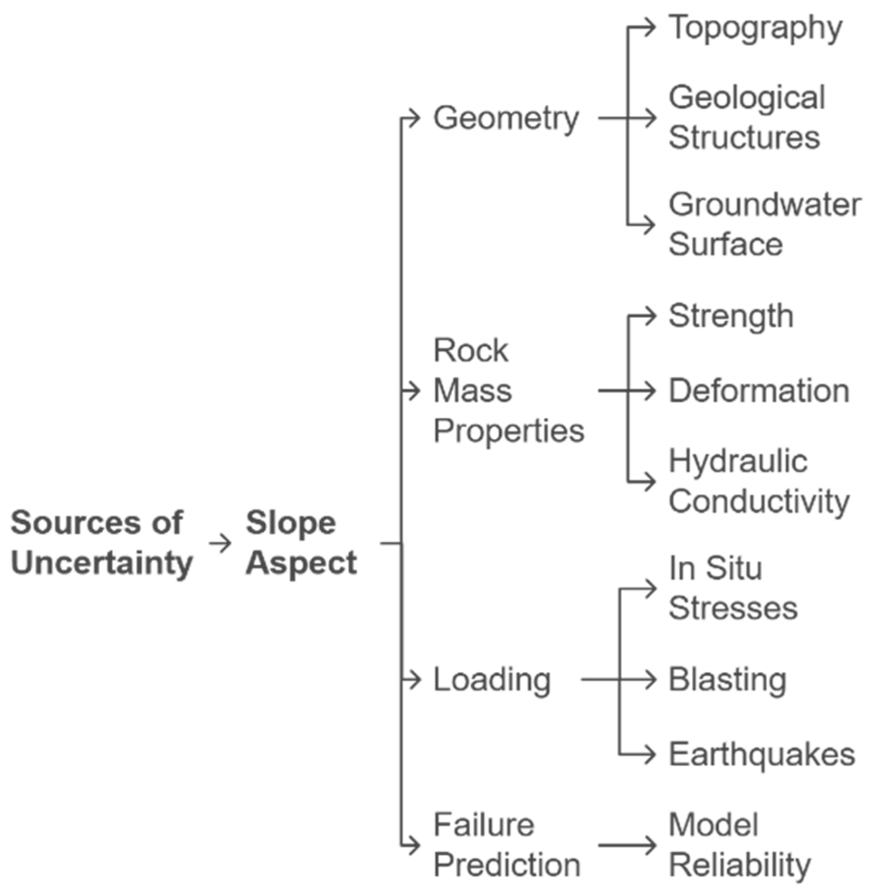
Figure 1. Flowchart for the sources of uncertainty when a particular slope is analyzed.
Geohazards 06 00067 g001
Figure 2. Schematic representation illustrating the parameters associated with the slope of an open-pit bench.
Geohazards 06 00067 g002
Figure 3. Geological structures result from the Earth’s crust deformation due to tectonic forces.
Geohazards 06 00067 g003
Figure 4. Flowchart illustrating the consequences of groundwater presence and heavy rainfall events.
Geohazards 06 00067 g004
Figure 5. Daily tasks in an open-pit operation can impact slope stability.
Geohazards 06 00067 g005
Figure 6. Illustration of a flowchart for a Decision Tree Technique, indicating that specific conditions regarding RMR, slope angle, joint spacing, and joint orientation can result in either a stable or unstable slope.
Geohazards 06 00067 g006
Figure 7. The graph illustrates the percentage distribution of various outputs in slope stability analysis.
Geohazards 06 00067 g007
Table 1. Overview of techniques to estimate the Factor of Safety.
FeatureMLP (Neural Network)SVR (Support Vector Regression)M5P (Model Tree Regression)
AccuracyHigh accuracy, especially for complex and nonlinear relationships.Performs well but may be sensitive to hyperparameter selection.Generally, accuracy is high, though slightly lower than MLP in complex scenarios.
Computational EfficiencyComputationally expensive, especially for large datasets, requires high-performance computing resources (e.g., GPUs).It is computationally efficient for small to medium datasets but can be slow for large-scale applications.Highly efficient; pruning techniques reduce complexity, making it the fastest model among the three.
InterpretabilityConsidered a “black box” model, difficult to interpret due to the complexity of neural network layers.It offers moderate interpretability, especially when using linear kernels. However, interpretability reduces with more complex kernels (e.g., RBF).Highly interpretable, as the model follows a structured decision tree format, with linear regression applied at leaf nodes.
Handles NonlinearityExcellent at capturing nonlinear relationships due to deep network architecture.Handles nonlinearity effectively through kernel functions (e.g., RBF, polynomial), but performance depends on kernel selection.Limited ability to capture nonlinearity; performs best in datasets with mostly linear relationships.
Handles Small DatasetsRequires a large dataset for practical training; prone to overfitting in small datasets.Well-suited for small datasets; capable of robust predictions with limited data points.Well-suited for small datasets; capable of robust predictions with limited data points.
Risk of OverfittingHigh risk of overfitting if not properly regularized (e.g., using dropout, L2 regularization).Lower overfitting risk due to margin-based optimization; generalizes well with appropriate kernel selectionModerate risk of overfitting but pruning techniques help maintain model generalization.
Table 2. Overview of techniques for classifying a slope as Stable or Unstable.
FeatureExtreme Gradient Boosting (XGBoost)Random Forest (RF)Support Vector Machine (SVM)P (Model Tree Regression)
AccuracyDemonstrates high classification accuracy, particularly in large datasets with complex relationships. Achieves strong performance due to boosting-based learning.It provides high accuracy but is slightly lower than XGBoost when handling highly nonlinear relationships.Offers high accuracy for small to medium datasets, but performance depends on kernel selection.
Computational EfficiencyModerate computational cost: optimized through parallelization and tree pruning, but still requires significant resources for large datasets.It is computationally expensive, especially with large datasets, due to multiple decision trees. Training is also slower than XGBoost.High computational cost for large datasets; solving quadratic optimization problems increases training time significantly.
Overfitting ResistanceIt incorporates regularization (L1 & L2) to prevent overfitting. It requires careful hyperparameter tuning to balance the bias-variance tradeoff.Resistant to overfitting due to averaging multiple decision trees. However, it may still overfit with excessive trees.Generally, less prone to overfitting, mainly when appropriate kernel functions are selected.
InterpretabilityConsidered a black-box model due to complex tree interactions, making it challenging to interpret feature contributions.Provides moderate interpretability through feature importance rankings.Low interpretability, especially for nonlinear kernels, makes it challenging to extract geotechnical insights.
Handling of Nonlinear RelationshipsEffectively captures nonlinear interactions through boosting, superior to Random Forest in complex decision boundaries.Moderate performance in nonlinear datasets; performs well but is less flexible than XGBoost for complex relationships.It is best suited for highly nonlinear datasets due to kernel-based learning, particularly with RBF and polynomial kernels.
Performance on Small DatasetsPerforms better on large datasets but may overfit small datasets without proper tuning.It requires a moderate dataset size to perform well; it may not be the best choice for very small datasets.It best suits small datasets, where SVM’s structural risk minimization ensures good generalization.
ScalabilityEffectively captures nonlinear interactions through boosting, superior to Random Forest in complex decision boundaries.Moderate performance in nonlinear datasets; performs well but is less flexible than XGBoost for complex relationships.Moderate performance in nonlinear datasets; performs well but is less flexible than XGBoost for complex relationships.
Robustness to Missing DataHandles missing values well by learning optimal splits; imputation is often unnecessary.Handles missing data moderately well but requires imputation in some cases.Sensitive to missing values; typically requires preprocessing and imputation before training.
Feature Importance AnalysisIt offers some feature importance insights but lacks interpretability compared to RF.The best model for feature importance analysis is one that quickly identifies key geotechnical parameters.Difficult to interpret feature contributions, particularly with kernel-based SVM models.
Disclaimer/Publisher’s Note: The statements, opinions and data contained in all publications are solely those of the individual author(s) and contributor(s) and not of MDPI and/or the editor(s). MDPI and/or the editor(s) disclaim responsibility for any injury to people or property resulting from any ideas, methods, instructions or products referred to in the content.