Modelling of Bottom Shear Stresses in Scoured Hole Formed by Nappe Flow During Levee Overtopping

Abstract

Increases in flood magnitude due to climate change increase the necessity of resilient river levees to prevent the breaching that can contribute to reduced flood inundation volume even when overtopping from a levee occurs. When a levee is composed of cohesive soil and the levee crest is paved, overtopping can lead to a waterfall-like nappe flow due to the erosion of the downstream slope of a levee. This flow subsequently expands the scour hole and increases the risk of levee failure. Although some models of scour hole expansion due to nappe flow were proposed, flow structures in the scour hole were not adequately taken into account. This study aimed to clarify the flow structure, including formation of vortices in the scour hole, by conducting flow visualization experiments and three-dimensional numerical analyses. After clarifying the flow structure, this study proposed a simplified model to calculate the bottom shear stress in a scour hole on the levee side. The accuracy of the estimated bottom shear stress was verified by comparing the results with a three-dimensional numerical analysis. This proposed method can predict further erosion of a scour hole.

1. Introduction

River floods are one of the most devastating natural disasters. Economic losses due to river floods are expected to increase in many regions due to economic growth, population increase, and climate change [1,2]. Although river levees increase the river flow capacity and reduce flood damage, their failures can cause significant damage in the hinterland. Although overtopping, erosion, seepage, and piping are well-known causes of levee breaches during floods, overtopping was often the primary factor [3,4,5,6,7].

The mechanism of a levee failure due to overtopping varies greatly depending on the levee material [8,9,10]. In the case of sand levees, overtopping flow erodes the entire back slope, particularly near the top, and begins to affect the crest [8,10]. Erosion of the full width of the crest decreases the height of the levee, allowing an increase in overtopping flow. Therefore, maintaining the height of the crest is crucial to prevent further inundation damage. In the case of clay levees, erosion occurs first along the back slope. Eventually, a headcut is formed, and an impinging jet (a nappe flow) forms at the crest of the levee. This nappe flow collides with the landing point, eroding the base of the levee and resulting in the formation of a scour hole and mass failure of the levee body [9,10]. For instance, overtopping was a main factor in the levee breach of the September 2015 Kinu River flooding by Typhoon Kilo [11,12], and a nappe flow formation was observed during the erosion of the inland slope [13]. Several large scour holes (pools dug) were formed by the overtopping up to approximately 5 m. The levee of the Kinu River at the levee failure point consisted of sandy silt to fine sand, and the crest was paved with asphalt.

A key goal in river levee improvement is preventing the river levee from being breached or delaying the time until a breach occurs, even if overtopping occurs. The Ministry of Land, Infrastructure, Transport and Tourism in Japan aims to develop a levee construction method that can withstand three hours of overtopping at 30 cm overflow depth [14]. Effective methods to extend the time before levee failure include covering the slope with turf grasses, impervious sheets, and grid materials that also reduce erosion on the back slope [15,16,17,18]. The crests of river levees should be paved to reduce rainwater infiltration and to improve the efficiency of river patrols, and this pavement has the effect of reducing erosion of the crest [19]. The pavement at the top of the levee not only reduces erosion of the crest but also keeps the nappe flow landing position far from the levee. With standard pavement rigidity, the pavement may bend and drop due to soil mass failure under the pavement. Therefore, increasing the rigidity of the pavement enhances effectiveness by keeping the distance of the nappe flow landing position over a longer period [20]. In addition, grid materials and drains can be used to dissipate the energy of the nappe flow as a way to extend the time until the levee is breached [21,22]. After a scour hole is formed by nappe flow, it is important to reduce the bottom shear stress to delay expansion of the scour hole.

Numerical simulations of levee erosion and modeling of levee breach mechanisms are important for assessing the risk of a levee breach and estimating the time to a breach. Many models of levee breaching have been developed, particularly for sand dikes (e.g., [8,23,24]). In contrast, there are only a few models for estimating a breach of clay (cohesive) levees (e.g., [19,25,26]. Zhu et al. [25] modeled the progression of scour depth due to the impact of an impinging jet on the bottom of the scour hole and the overturning failure of the headcut soil mass. The equation of Stein et al. [27] was used for the increase in scour depth. Stein et al. [27] calculated the bottom shear stress ($\tau$) from a jet velocity (U_B) around the bottom of a scour hole as shown in

Table 1. Comparing the methods of calculation of the bed shear stress in the scour hole.

	Stein et al. [27]	Palermo et al. [28]	Our Study
Method of calculation for the bed shear stress in the scour hole: τ	Using the friction coefficient (Cf) and the impinging flow velocity around the bottom of scour hole (UB). $\hspace{1em}\hspace{1em}\hspace{1em}\hspace{1em}\hspace{1em}\hspace{1em}\hspace{1em}\tau =C_f\rho U_B^2$ UB is calculated taking into account diffusion within the scour hole. $\hspace{1em}\hspace{1em}\hspace{1em}\hspace{1em}\hspace{1em}\hspace{1em}{U}_B=C_d\sqrt{{\displaystyle \frac{T_{Nf}}{J}}}{U}_0$ where, Cd is diffusion constant of a jet, U0 is jet velocity at the water surface, TNf is jet thickness at the water surface, J is the scour hole depth (J) along the jet centerline.	Based on the angular-momentum conservation law to rigid bodies. $\hspace{1em}\hspace{1em}\hspace{1em}\hspace{1em}\hspace{1em}\hspace{1em}\hspace{1em}{T}_{zM}-T_{z\tau }=I_z{\displaystyle \frac{d\omega }{dt}}=0 (\because \omega \mathrm{i}\mathrm{s} \mathrm{c}\mathrm{o}\mathrm{n}\mathrm{s}\mathrm{t}\mathrm{a}\mathrm{n}\mathrm{t})$ Different point 1: The study focused on a main large vortex (vortex A). $T_{zM}$ is a torque of the moment flux of the jet $\left(\rho QV\right)$. R is a moment radius. $\hspace{1em}\hspace{1em}\hspace{1em}\hspace{1em}\hspace{1em}\hspace{1em}\hspace{1em}\hspace{1em}\hspace{1em}\hspace{1em}{T}_{zM}~\left(\rho QV\right)R$ Different point 2: The study assume the vortex is a cylinder shape. Therefore, same moment radius with the torque of jet was used to calculate a torque of the shear force $T_{z\tau }$$. \theta RB$ is the area that shear stress acts on. $\hspace{1em}\hspace{1em}\hspace{1em}\hspace{1em}\hspace{1em}\hspace{1em}\hspace{1em}\hspace{1em}{T}_{z\tau }~\left(\tau \theta RB\right)R \therefore \tau \cong {\displaystyle \frac{\rho QV}{RB}}$ Different point 3: The velocity before water landing is used as V.	Based on the angular-momentum conservation law to rigid bodies as shown in Equation (3). Different point 1: Our study focused on a secondary levee side vortex (vortex B). Therefore, a coefficient k1 was introduced as shown in Equation (4). Different point 2: The moment radius used to calculate the shear force torque was $R_2\left(\theta \right)$ instead of $R_1$ because vortex B was not cylindrical in shape. $\hspace{1em}\hspace{1em}\hspace{1em}\hspace{1em}\hspace{1em}\hspace{1em}{T}_{z{\tau }_1}={\int }_0^{\theta }{R}_2\left(\theta \right)\cdot \tau B{R}_2\left(\theta \right)d\theta$ Therefore, Equations (5), (8), and (9) are derived. Different point 3: Both the mean velocity ($V_{1ave}$, Equation (7)) and the maximum velocity $V\left(x_1\right)$ were considered for $V_1$.
Calculated value of τ (N/m2)	5.0	156.2	0.35 (when $V_1=V\left(x_1\right)$) 0.18 (when $V_1=V_{1ave}$)

. U_B is calculated from the jet velocity (U₀) just before landing on the water surface, the jet thickness (T_Nf), and the scour depth along the jet centerline, taking into account the diffusion of the flow within the scour hole. The jet velocity along the centerline is assumed to be constant for some distance (within the length of the potential core) after the jet enters the scour hole. After the calculation of $\tau$, the increase in the scour hole depth over time from the excess shear stress (=$\tau$ − the critical shear stress) is calculated. Similarly, D’Eliso [26] used the equation of Stein et al. [27] to calculate scour depth. When the scour depth is shallow, it is natural to calculate the increase in scour depth by using impinging jet velocity around the bottom. On the other hand, the following assumptions are questionable for a jet entering a relatively small scour hole, or, in other words, for a jet affected by the boundary:

• the existence of a potential core with a constant jet velocity;
• the scour depth is calculated based on the jet velocity, even when the scour depth has sufficiently enlarged to exceed the potential core length.

Kainose et al. [20] assumed the occurrence of Rankine vortices in the scour hole and calculated erosion using the velocity at the bottom of the scour hole caused by the Rankine vortices. Although the occurrence of a Rankine vortex in the scour hole and the radius of the forced vortex have not been experimentally verified, it is important to consider the flow structure in the scour hole. Palermo et al. [28] evaluated the bottom shear stress in a scour hole induced by a jet vortex using conservation of the angular momentum. Because the study focused on maximum scour depth, it considered only one large vortex. However, a small vortex of opposite rotation is more significant because the erosion of the lower part of the headcut is primarily affected by this small vortex in the levee failure mechanism.

Therefore, this study first clarified in detail the flow structure in one scour hole through particle image velocity (PIV) experiments and three-dimensional numerical analysis using OpenFOAM. This approach aimed to elucidate the jet behavior in the scour hole, the existence of a potential core, and conditions of the vortices. Subsequently, a model of the bottom shear stress is proposed to quantitatively evaluate the scour expansion process considering the flow conditions in the scour hole.

2. Materials and Methods

2.1. Flow Visualization with Particle Image Velocimetry

In the PIV experiment, a rigid bed with a scour hole and a post-erosion levee model of the back slope was set up in a circulating open channel measuring 6.5 m in length, 0.5 m in width, and 1.2 m in depth, as shown in Figure 1a. The shape of the scour hole was based on measurements taken 25 min after overtopping with 2 cm overflow depth (h) at the center of the crest in a previous flume experiment [18], in which scour depth (H_S) was 35 cm as shown in Figure 1b. This represents the shape of the scour hole just before the scour depth reached the maximum (before the soil mass failure of the levee body occurred). For generalizing the quantification of the scouring, an analysis of various scour hole shapes is required corresponding to the expansion process. However, considering the complex flow pattern change in the time series, this study used a scour hole shape in which the vortex structures were stable (after the scour hole has expanded sufficiently) as a first step in clarifying the flow structure in a scour hole. In this previous experiment, the levee material was Mikawa silica sand No. 8, and the physical scale of the experiment was set as 1/10, assuming a river levee with a height of 3 m in actual scale.

The variable h was set as 2 cm, 3 cm, and 4 cm for three different cases in our study because the actual overflow depth is often 20 cm to 40 cm [12]. Assuming that h is the critical water depth, for h = 2, 3, and 4 cm, the flow rates per unit width (q) were 0.0089, 0.0163, and 0.0251 m²/s, respectively, and the corresponding flow velocities were 0.44, 0.54, and 0.63 m/s, respectively. Assuming a horizontal projection of a rigid body at this velocity, the velocities ($U_0=\sqrt{\mathrm{g}\left(0.3+h\right)}$) just before the landing point were 2.47, 2.49, and 2.51 m/s for h = 2, 3 and 4 cm, respectively. Here, g is the acceleration of gravity, and 0.3 m is the height of levee model (H_L). As mentioned above, the scour hole shape was formed with h = 2 cm; however, our PIV experiments were also conducted with h = 3 cm and 4 cm. This is based on the assumption that the actual overtopping is a non-steady phenomenon and that the overflow depth varies with time. In other words, this experiment assumes that the scour is sufficiently enlarged at h = 2 cm, and then the overflow depth increases up to 3 cm or 4 cm.

As shown in Figure 1a, the PIV laser was installed inside the fixed bed downstream of the scour hole. This is because accurate results cannot be obtained when the laser beam is directed from above the oscillating water surface due to issues with reflection and refraction. Acrylic glass was used as a slit to allow the laser beam to enter the scour hole. The laser beam was placed 10 cm from the sidewall of the channel. The transport of tracer particles reflecting from the laser beam was recorded as particle images at a frame rate of 200 frames per second (fps). To prevent degradation of image quality, the particle images were captured from two angles: upstream (x = −9 cm to 26 cm, y = −2 cm to 22 cm) and downstream (x = 13 cm to 48 cm, y = 5 cm to 30 cm) of the scour hole. The particle images (5580 frames at 200 fps) were analyzed using the software “Flow Expert64 Ver.1.2.6” (Kato Koken Co., Ltd., Kanagawa, Japan) to calculate the particle velocities. The 5580 frames of the particle images were divided into approximately 500 frames each and analyzed to obtain data on 11 velocity distributions for each case. The mean values and standard deviations of the landing position of the nappe flow and the vortex center position, which will be discussed later, were calculated from these 11 data sets.

2.2. Three-Dimensional Numerical Analysis Using OpenFOAM

As will be mentioned later, the accuracy of measurements near the bottom of scour hole was low in the PIV experiment. To quantitatively assess the risk of a levee breach, it is important to evaluate the flow velocity and shear stress near the bottom. Therefore, this study attempted to reproduce the flow condition using a three-dimensional fluid analysis model in OpenFOAM. The interFoam solver, an OpenFOAM algorithm that can calculate the water–air interface using a volume of fluid (VOF) method, was used. In this study, a hybrid technique, DES (detached eddy simulation), which uses RANS (Reynolds-averaged Navier–Stokes) near the wall and LES (large eddy simulation) away from the wall, was adopted as shown in Equations (1) and (2).

$${\displaystyle \frac{\partial {\overline{u}}_i}{\partial x_i}}=0$$

(1)

$${\displaystyle \frac{\partial {\overline{u}}_i}{\partial t}}+{\displaystyle \frac{\partial \left({\overline{u}}_i{\overline{u}}_j\right)}{\partial x_j}}=-{\displaystyle \frac{1}{\rho }}{\displaystyle \frac{\partial \overline{p}}{\partial x_i}}+{\displaystyle \frac{\partial }{\partial x_j}}\left[\nu \left({\displaystyle \frac{\partial {\overline{u}}_i}{\partial x_j}}+{\displaystyle \frac{\partial {\overline{u}}_j}{\partial x_i}}\right)-{\tau }_{ij}\right]$$

(2)

where ${\overline{u}}_i$ is the mean flow velocity, $\overline{p}$ is the pressure, $\rho$ is the density of the fluid, and $t$ is time. ${\tau }_{ij} \left(=\overline{u_i{u}_j}-{\overline{u}}_i{\overline{u}}_j\right)$ is defined as Reynolds stress in the RANS domain and SGS (subgrid scale) stress in the LES domain and is an unknown that must be obtained from a turbulence model. This study used the k-ωSST model as a turbulence model, which switches between the k-ε model and the k-ω model depending on the distance from the wall. The model has been confirmed to have high calculation accuracy for near-bottom flow, which affects the erosion of the scour hole, and low error compared to actual phenomena [29].

For the OpenFOAM simulations, a model with the same geometry as the PIV experiment was created. The mesh size was set to 2 cm, basically, and refined to 5 mm from the center of the levee crest throughout the entire scour hole. The PIV experiment for h = 4 cm indicated that the thickness of a nappe flow (T_Nf) just before impingement to the scour hole was 2.4 cm. The refined mesh size, 5 mm, was set to divide this thickness (T_Nf) into approximately five sections. Because the values of T_Nf are smaller for h = 2 cm and 3 cm cases, a finer mesh size is required. In the simulation for a channel width of 50 cm, a mesh size finer than 5 mm could not be implemented due to the computational load and the upper limit on the number of meshes; therefore, only h = 4 cm was tested in this study. The computation time step was automatically adjusted and set so that the maximum Courant number was less than 1. The non-slip condition was used at the wall boundary to reproduce the sidewall of the channel by setting the flow velocity to zero.

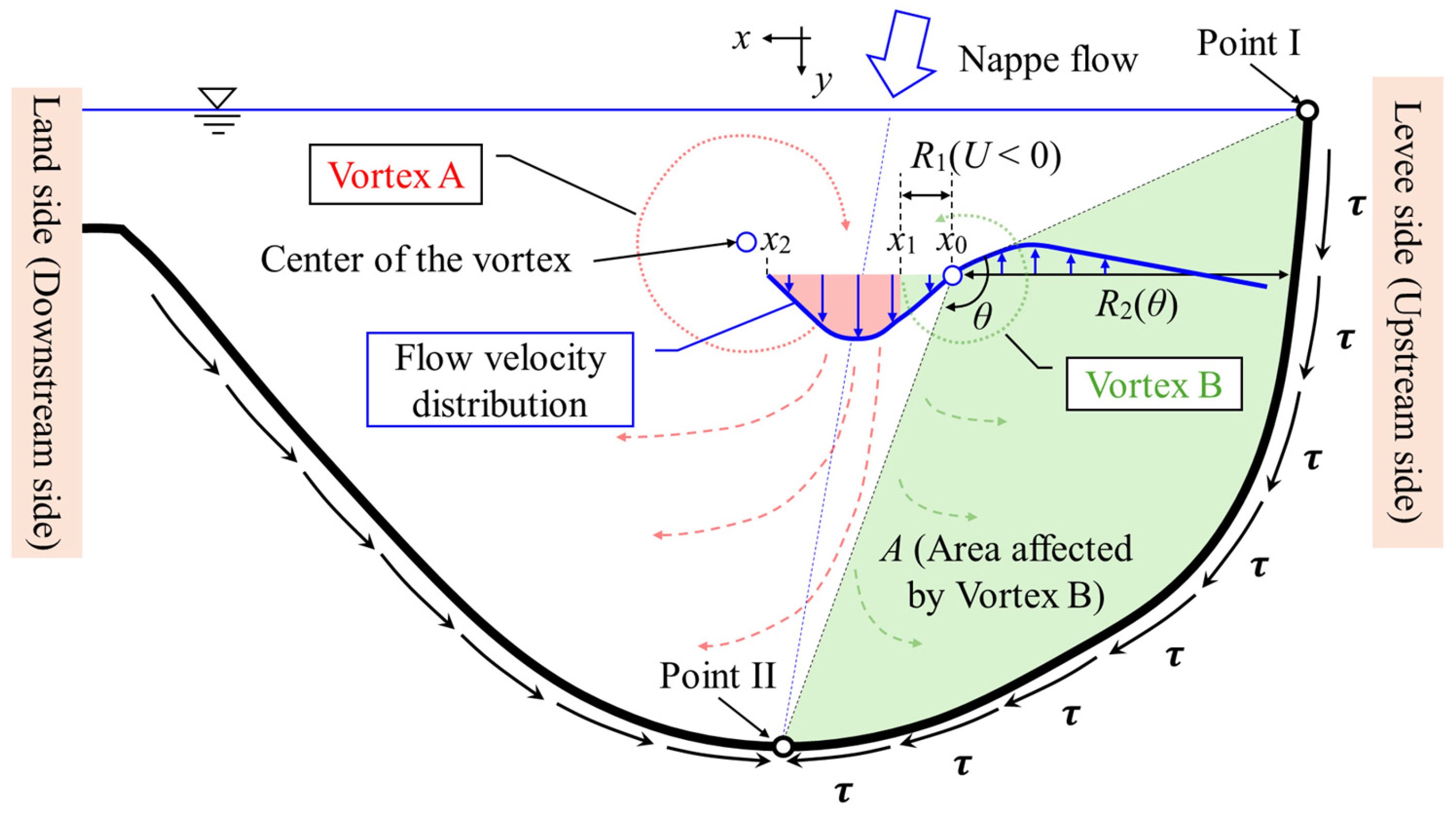
2.3. Modeling of Bottom Shear Stresses in Scour Hole

As already mentioned, one large vortex due to the jet flow considered by Palermo et al. [28] corresponds to the clockwise vortex A as shown in Figure 2. The counterclockwise vortex B on the levee side and the bottom shear stress due to vortex B are more important when discussing the risk of levee failure. As shown in Table 1, Palermo et al. [28] used the well-known equation of angular-momentum conservation for one main vortex (Vortex A in Figure 2). Because the angular velocity of the vortex (ω) is constant, the torque due to the momentum flux of the jet is balanced by the torque due to the shear force. The momentum radii used in the two torque calculations are both R because the vortex structure is assumed to be a cylinder. The energy loss of the jet due to the water landing is ignored, and the velocity before the water landing is used for the calculation of the momentum flux of the jet.

The basic hypothesis of our study is similar to that of Palermo et al. [28], and an angular momentum conservation law (Equation (3)) was used. There are three main differences between Palermo et al. [28] and our study, as shown in Table 1. First, the vortex in focus is not the main vortex (vortex A), but the secondary vortex (vortex B). Therefore, the momentum flux of the jet shown in Equation (4) is multiplied by coefficient k. Second, the vortex structure is not a cylinder, and the center of vortex B is close to the centerline of the jet. This is based on the analysis of the PIV experiment and three-dimensional analysis by OpenFOAM. Therefore, the different momentum radii are used for the calculation of the two torques. Third, the velocity used to calculate the momentum flux of the jet is the velocity at the height of the center of vortex B. This velocity takes into account the energy loss due to the water landing of the nappe flow.

$$T_{z{M}_1}-T_{z{\tau }_1}=I_z{\displaystyle \frac{d\omega }{dt}}$$

(3)

where $T_{z{M}_1}$ is torque due to the nappe flow that forces vortex B (Equation (4)), and $T_{z{\tau }_1}$ is torque due to shear stress $\tau$ (Equation (5)). The right-hand side of Equation (3) represents the change in time of the angular momentum of vortex B and is zero because the angular velocity $\omega$ of vortex B is constant.

$$T_{z{M}_1}=k_1\left(\rho Q{V}_1\right)R_1$$

(4)

where k₁ is the ratio of the moment flux that forces vortex B and that of the impinging jet of the nappe flow calculated by Equation (6), $\rho$ is the density of water, $Q$ is the flow rate, $V_1$ is the velocity of the impinging jet, and $R_1$ is the radius of vortex B (=$x_1-x_0$). An analysis of the OpenFOAM results shows that the value of k₁ is 0.087 (the details will be described later), which means that 91.3% and 8.7% of the jet moment fluxes contributes to driving vortex A and vortex B, respectively.

For the torque due to shear stress, $T_{z{\tau }_1}$, can be modeled as,

$$T_{z{\tau }_1}=\tau B{\int }_0^{\theta }{R}_2{\left(\theta \right)}^{2}d\theta$$

(5)

where $\tau$ is the bottom shear stress on the levee side, $B$ is the channel width, $\theta$ is the angle from the intersection of the water surface and bottom of the scour hole (Point I) to the deepest point of the scour hole (Point II) with respect to the center of vortex B, and $R_2\left(\theta \right)$ is the distance from the center of vortex B to the bottom of the scour hole as a function of angle $\theta$. Considering the small angle ($d\theta$), the area where the shear stress ($\tau$) acts is $B{R}_2\left(\theta \right)d\theta$.

Therefore, integrating the torque into the angle from 0 to θ yields Equation (5).

$$k={\displaystyle \frac{{\int }_{x_0}^{x_1}V\left(x\right)dx}{{\int }_{x_0}^{x_2}V\left(x\right)dx}}$$

(6)

where $V\left(x\right)$ is the flow velocity in y direction at position x. The section of the impinging jet that forces vortex B (from $x_0$ to $x_1$) is determined from the range in which the flow velocity in x direction where U is negative. The flow velocity U is positive from $x_1$ to $x_2$.

In this study, both the mean velocity (Equation (7)) and the maximum velocity $V\left(x_1\right)$ were considered for $V_1$. This is because the nappe flow velocity just before water landing (U₀) and the jet velocity just after water landing were significantly different. In other words, if U₀, which does not include energy loss due to water landing, is considered as a driving velocity of the vortex, the error of the shear stress can be large.

$$V_{1ave}={\displaystyle \frac{1}{R_1}}{\int }_{x_0}^{x_1}V\left(x\right)dx$$

(7)

Assuming that the area affected by the vortex B is A, Equation (5) can be modified as Equation (8).

$$T_{z\tau }=\tau BA$$

(8)

Therefore, the bottom shear stress τ on the levee side of the scour hole can be expressed by Equation (9).

$$\tau ={\displaystyle \frac{k_1\left(\rho Q{V}_1\right)R_1}{BA}}$$

(9)

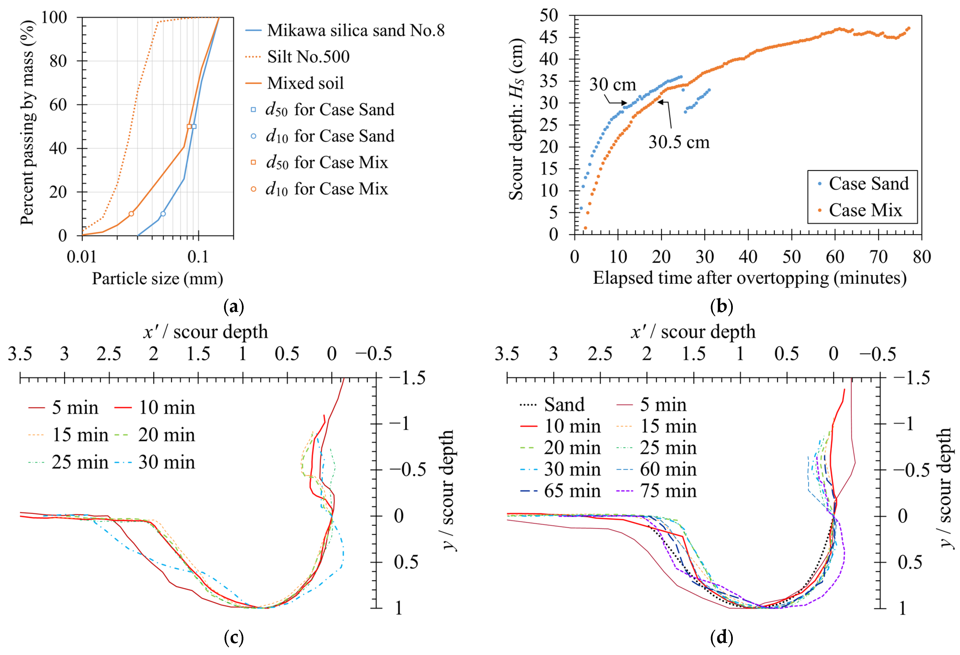
2.4. Previous Experiments on Levee Erosion by Nappe Flow to Compare with the Proposed Method

The proposed method in our study was developed based on the flow visualization using PIV experiments and the results of OpenFOAM analysis for the limited conditions (hereinafter called reference conditions) in which H_L is 30 cm, h is 4 cm, H_S is 35 cm, and levee material is Mikawa silica sand No. 8. For validating the accuracy of the estimated bottom shear stress, our model was applied to two cases of the previous experiments that are different from the reference conditions. The previous experiment was an erosion experiment due to levee overtopping conducted by Onose et al. [30]. H_L was 30 cm, h was 2 cm, H_S changed over time, and two types of soil material were tested. Figure 3a shows the grain size distribution of the soil materials used in the previous experiments [30]. The soil materials in Case Sand and Case Mix contained 100% Mikawa silica sand No. 8 (d₅₀ = 0.0917 mm and d₁₀ = 0.0495 mm where d₅₀ and d₁₀ represent the grain diameters for 50% and 10% finer soil particles) and a mixed soil (d₅₀ = 0.0831 mm and d₁₀ = 0.0263 mm) of Mikawa silica sand No. 8 and silt No. 500 in a ratio of 4:1, respectively. Figure 3b–d summarized the results of previous experiments. For both cases, the scour depth increased rapidly for about the first 10 min after overtopping. After that, the scour depth continued to increase, but the rate of increase in the scour depth decreased. In Case Sand, the scour depth became small at approximately 25 min. This is a result of refilling the scour hole with soil mass caused by failure of a part of the levee body. In Cases Sand and Mix, the soil mass below the levee crest collapsed completely at 31 min and 77 min, respectively.

Figure 3c,d show the non-dimensional scour hole shapes at each time for Case Sand and Case Mix, respectively. The vertical axis is the nondimensional value, which is the y value as shown in Figure 1 divided by the scour depth at each time. For the horizontal axis, the value is taken as a parallel translation so that x’ = 0 when the upstream end of the scoured region is 0, and then x’ is divided by the scour depth. Figure 3c shows that the non-dimensional scour hole shapes at 10, 15, 20, and 25 min are almost identical. At 5 min, the early stage of overflow, the scour hole shape is not only determined by the nappe flow, but also by the effect of scouring near the toe of the levee due to the flow along the levee slope. Therefore, the nondimensionalized scour depth of the land side at 5 min was deeper than that of 10 to 25 min. The shape at 30 min is a little different due to the sedimentation falling into the scour hole just after the soil mass failure. Figure 3d also shows the average shape of Case Sand from 10 to 25 min and the non-dimensional scour shape in Case Mix at each time. Although, the soil material of Cases Sand and Mix is different, the shape is similar. These results show that the scour hole shape of the reference condition of our proposed model was similar regardless of the scour depth and soil material except just after overtopping or soil mass failure.

To calculate the affected area A in Equation (9), the following relationship (Equation (10)) between the scour hole depth (H_S) and A was used.

$$A=k_2{H}_S^2$$

(10)

where k₂ is a coefficient related to the scour hole shape, and k₂ = 0.536 under the reference conditions. The same k₂ could be used for the previous experiments [30] because the scour hole shape was similar. In addition, it was assumed that the k₁ and R₁/H_L are constant regardless of the scour depth. To judge whether the scour hole erosion is progressing or not, V(x₁) should be used as V₁ in Equation (9). V(x₁) is considered to be proportional to the vertical flow velocity just before the water landing as shown in Equation (11).

$$V\left(x_1\right)=k_3\sqrt{\mathrm{g}{H}_L}$$

(11)

where k₃ is the coefficient related to the energy loss due to the water landing, and k₃ = 0.309 for the reference conditions. In previous experiments [30], the overflow water depth was different from the reference conditions, but the embankment height was the same. It is considered that the difference in the vertical flow velocity just before the water landing due to the difference in the overflow water depth can be ignored, and thus k₃ is set to 0.31. Therefore, Equation (9) can be modified as Equation (12).

$$\tau ={\displaystyle \frac{k_1{k}_3\rho Q\sqrt{\mathrm{g}{H}_L}{R}_1}{k_{2}B{H}_S^2}}=0.00334\rho q{\displaystyle \frac{\sqrt{\mathrm{g}{H}_L^3}}{H_S^2}}$$

(12)

3. Results

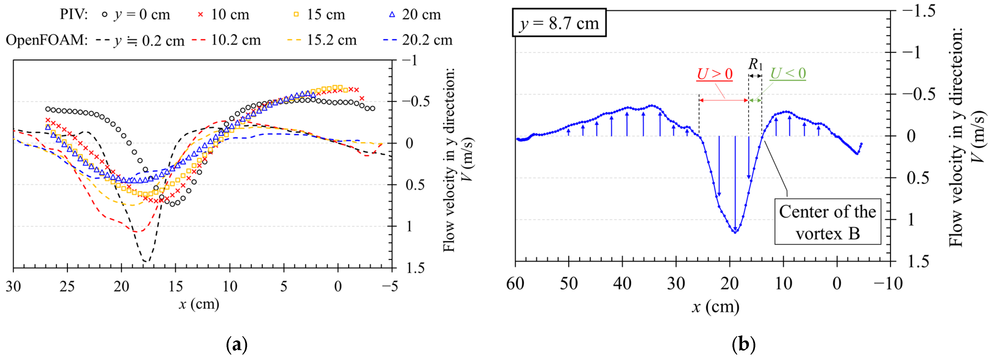
3.1. Results of PIV Experiments

Figure 4a–c show the time-averaged flow velocity vectors analyzed from PIV taken upstream of the scour hole for the cases of h = 2 cm, 3 cm, and 4 cm, respectively. In the flow visualization, two vortices were clearly observed on the levee side and the land side of the impinging jet in all cases despite the complex flow field in the scour hole. This is because the positions and sizes of the two vortices do not change significantly over time, and the two vortices are formed without any interruption in time. Although the center of the vortex on the landward side cannot be confirmed in Figure 4b, the vortex was clearly reproduced in the particle image taken at the downstream angle. A high-velocity region was observed after the impingement of nappe flow. Although the jet velocity of this region was not constant and gradually decreased, this region is similar to the potential core. Velocity vectors were observed only near the bottom in a direction different from the visually observed flow, e.g., the flow toward the bottom (as shown by the yellow dashed line in Figure 4). This is because the PIV laser beam is reflected near the bottom of the scour hole and the tracer particles in the fluid cannot follow the trajectory. The PIV results within this dashed line are not discussed further because they are inaccurate.

Figure 5 shows the height of the levee crest and the bottom of the scour hole, the location of the vortex center analyzed from the PIV, the location of the maximum jet velocity at each height y (cm), and the estimated center of the nappe flow before the impingement. The center of the vortex is defined as the position where the flow velocity is the smallest inside the closed streamlines. The nappe flow centerline (dotted curves) shown in Figure 5 represents a parabola when the horizontal projectile of the mass point (initial velocity $\sqrt{gh}$) is considered. It should be noted that this dotted parabola before water landing is not the result of the PIV experiment, but an estimate based on the horizontal projectile assumption. In addition, observed results of the centerline of the nappe flow (dashed curves) are also shown in Figure 5. The landing position of the nappe flow and the position of the maximum jet velocity near the water surface were almost identical for h = 4.0 cm. On the other hand, for h = 2.0 cm and 3.0 cm, the maximum jet velocity near the water surface was shifted to the left (about 5 cm for h = 2 cm and 3 cm for h = 3 cm). This is caused by the air pressure trapped inside the nappe flow and the levee. Since air entrainment was observed due to the jet impingement regardless of the overflow depth, the air pressure trapped inside is considered to be increasing. The smaller the overtopping depth, the farther the position of the high-velocity region was generated from the landing position of the parabola of the horizontal projectile. This means that the smaller the overtopping depth, the more easily the nappe flow is shifted.

Regardless of the overflow depth, the center of vortex B is deeper than that of vortex A. The horizontal distance from the position of maximum jet velocity to the vortex center did not change significantly with overflow depth, and was about 5–6 cm. The standard deviation of the vortex center was small for h = 2.0 cm, while it was larger for h = 4.0 cm, particularly for vortex B. This indicates that the position of the vortex center, especially its height, tends to fluctuate over time. As already described, the scour shape used in the PIV experiment was obtained from the levee erosion experiment for h = 2.0 cm, when the scour depth is almost maximum. Therefore, the standard deviation was small for h = 2.0 cm because the vortex center was almost stable, while the jet velocity did not decrease sufficiently at the deepest part of the scour hole for h = 4.0 cm, and the center of the vortex was unstable and oscillated.

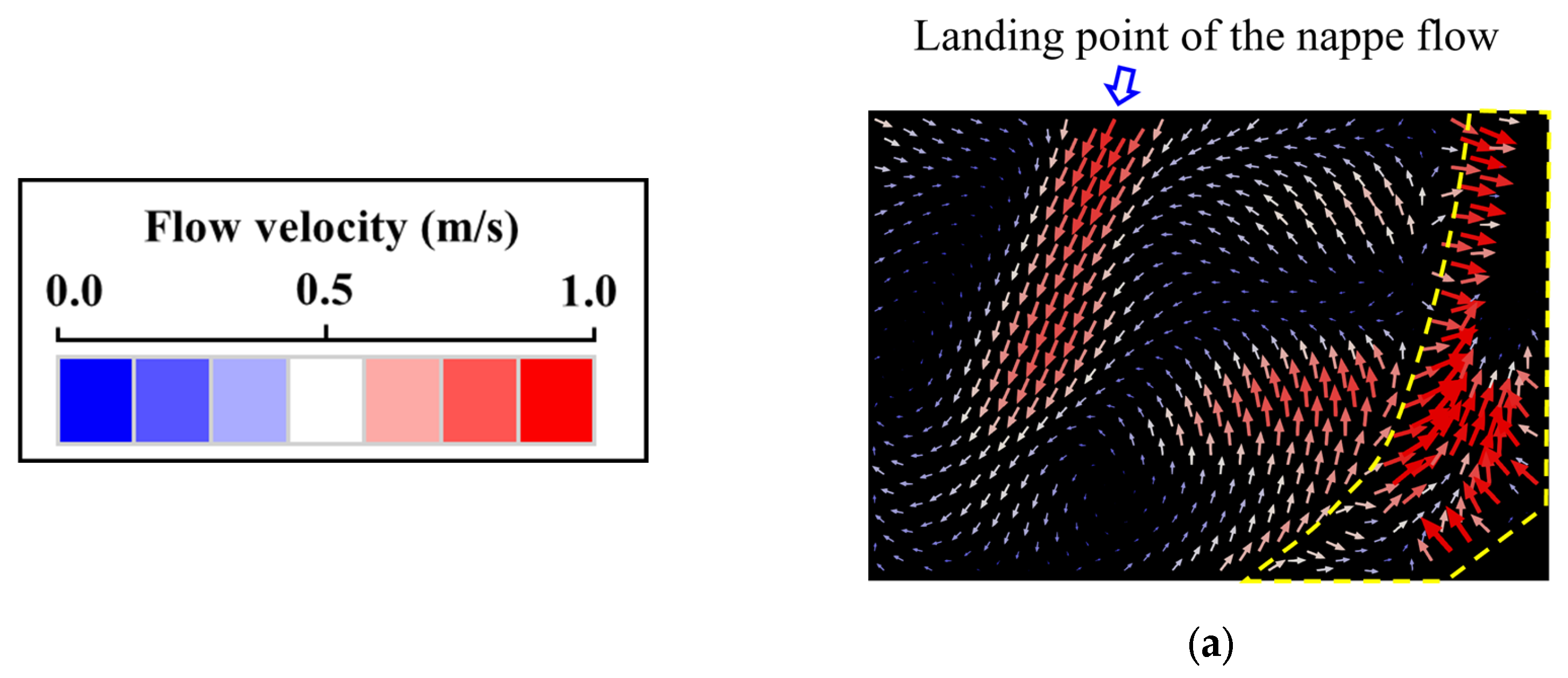
3.2. Results of Three-Dimensional Numerical Analysis with OpenFOAM

Figure 6 shows the velocity vector simulated by the OpenFOAM analysis for h = 4 cm. The area enclosed by the dashed line in Figure 6 represents the location of the angle of view for the PIV analysis in Figure 4c. In the simulation, the time-averaged velocity vectors shown in Figure 6 represent the average of the instantaneous velocity vectors taken at 0.2 s intervals from 10 to 20 s, when the flow stabilizes. This stabilization results from the historical effects of the initial conditions (waterlogging in the scour hole) during the first 10 s of the simulation. Two vortices observed in experiments were clearly reproduced in the numerical simulation. Comparing the PIV experiment with the OpenFOAM results, the horizontal distance Ld from the top of the back slope to the water landing point was 18 cm for OpenFOAM and 15.3 cm for PIV. Although Ld was slightly (3 cm) larger for OpenFOAM, the angles of nappe flow just before impingement were similar. The center of vortex B was y = 8.7 cm for OpenFOAM and y = 14.1 cm for the PIV experiment, which was about 5 cm shallower in OpenFOAM, within the mean value (14.1 cm) − standard deviation (6.1 cm) of the vortex center position in the PIV experiment. OpenFOAM reproduced the flow pattern well within a reasonable limit.

Figure 7a shows a comparison of the velocity distribution results of PIV experiment and OpenFOAM analysis at h = 4 cm. The maximum velocity at the centerline of the jet was slower in the PIV experiment than in the OpenFOAM analysis, especially at y = 0 cm just after the water landing. There are two possible reasons for this difference. One is the measurement error in the PIV experiment. In particular, the number of air bubbles just after water landing is large, and the measurement error can become large. Another one is that the velocity can be actually reduced by the air entrainment (buoyancy of bubbles) in the PIV experiment. The PIV results show that the maximum velocity of the jet after landing was 0.83, 0.80, and 0.73 m/s at h = 2, 3, and 4 cm, respectively. The smaller the overflow depth, the higher the measured maximum velocity of the jet after water landing. This result strengthens the credibility of the two reasons mentioned above. On the other hand, the maximum jet velocities of PIV and OpenFOAM were similar in the deeper parts of the scour hole, e.g., y = 15 and 20 cm, and the velocity profiles were similar in shape. This suggests that the OpenFOAM analysis is generally accurate. However, a weak upward velocity of about V = −0.5 m/s was measured at the levee side (x < 10 cm) in the PIV results, whereas it was about −0.1 m/s in the OpenFOAM results. This can be due to the effect of air bubbles, which is an issue for further investigation.

Figure 7b shows the vertical velocity (V) distribution in the horizontal plane passing through the center (x, y) = (14.0, 8.7) of vortex B shown in Figure 6. The high-velocity downward flow (positive in the y-axis) was observed in the scour hole, within the x range of 14 to 25.5 cm, following the landing of the nappe flow. When x = 9.5 cm, the flow velocity (V) was at a minimum (in other words, the flow velocity in the vertical upward direction was at a maximum). As shown in Figure 4 and Figure 6, the vortex generated by the nappe flow in the scour hole is not a perfectly circular shape. The vortex resembles a Rankine vortex, featuring a forced vortex section around the center and a free vortex section outside of it, where the velocity decreases inversely proportional to the distance from the center. In the high-velocity region, (x = 14–25.5 cm) due to the impinging jet, the x-directional flow velocity U < 0 for x = 14–16 cm and U > 0 for x = 16.5–25.5 cm. Therefore, $x_0$ = 14.0 cm, $x_1$ = 16.0 cm, $x_2$ = 25.5 cm, and $R_1$ = 2.0 cm in this case, and k₁ = 0.087 from Equation (6). This means that less than 1% of the high velocity flow generated vortex B.

4. Discussion

Figure 8 shows the bottom shear stress calculated from OpenFOAM and our proposed method. The OpenFOAM bottom shear stresses are the time-averaged values from 10 to 20 s and are the values at the center of the channel in the cross-stream direction. The critical tractive force $\rho {u_{\ast c}}^2$ calculated from Iwagaki’s formula [31] is also shown for Mikawa silica sand No. 8. The bottom shear stress calculated by OpenFOAM was less than the critical tractive force for x in the range of −0.06 m to 0.14 m and 0.28 m to 0.64 m, while it exceeded the critical tractive force in other sections. This indicates that scouring was nearly stopped throughout the entire scour hole; however, it was still ongoing near the maximum scour depth and at both ends of the scour hole. Although the depth of the scour hole used for this simulation was set as the maximum scour depth for h = 2 cm, the bottom shear stress was larger than the critical tractive force because this study was simulated by h = 4 cm.

As shown in Table 1, the bed shear stress calculated by the method of Palermo et al. [28] was extremely large (156.2 N/m²). This is because their method focused on a main strong vortex (vortex A), and the energy loss due to the water landing was not considered. In addition, the bottom shear stress calculated by the method of Stein et al. [27] was also large (5.0 N/m²). In this method, the energy loss from the water landing was not considered. In addition, the jet velocity is assumed to be constant in the potential core length (15 cm in this experiment condition). In fact, the jet velocity is reduced by about 16–48% in both the PIV measurement and the OpenFOAM analysis, as shown in Figure 7a. This assumption regarding the potential core length may have led to an overestimation of the jet velocity at the bottom of the scour hole and the bed shear stress. On the other hand, the bottom shear stress calculated by the proposed method in our study was 0.18 N/m² when the average value (Equation (7)) was used as V₁. This value was close to the average bottom shear stress of 0.14 N/m² on the levee side (x = −0.08–0.24 m) by OpenFOAM. When the maximum value of V(x₁) was used for V₁ in the proposed model, the bottom shear stress was 0.35 N/m², which was close to the maximum value of 0.3–0.42 N/m² for the bottom shear stress by OpenFOAM. This indicates that, in the proposed model, the average value used for V₁ can represent the average shear stress in the levee-side scour hole, while the maximum value for V₁ can represent the local shear stress near the maximum scour depth or at the edges of the scour hole. Comparing these shear stresses to the critical tractive force revealed that the mean shear stress of 0.18 N/m² was close to the critical tractive force of 0.16 N/m², indicating that erosion in the scour hole was subsiding on average. On the other hand, the local shear stress of 0.35 N/m² was more than double the critical scouring force, indicating that erosion was progressing locally.

The results of calculating the bottom shear stress using Equation (12) for Case Sand and Case Mix of the previous experiments [30] are shown in Figure 9a and Figure 9b, respectively. The critical tractive forces $\rho {u_{\ast c}}^2$ calculated from Iwagaki’s formula [31] are also shown for d₅₀ and d₁₀ of Cases Sand and Mix. Figure 9a,b show that τ became less than $\rho {u_{\ast c}}^2$ when H_S became larger than 0.30 m and 0.305 m in the Cases Sand and Mix, respectively. In this deep scour condition, particles larger than d₅₀ were less likely to be eroded. In the previous experiments [30], the erosion speed also decreased when the scour depth became approximately 30 cm, as shown in Figure 3b. Although the erosion rate is slowing, erosion is still progressing because the soil finer than d₅₀ can be eroded. In both cases, τ when H_S are the maximum, they are slightly larger than the $\rho {u_{\ast c}}^2$ for d₁₀, and these H_S represent the terminal scour depth. Our proposed model shows applicability to different overflow depths, scour depths, and soil materials. Future studies are needed to assess the model’s adaptability to various scour hole geometries and levee height. Abbas and Tanaka [21] showed that erosion due to a nappe flow landing can be reduced by using a geogrid material. Our study also shows that reducing the jet momentum flux through energy loss contributes to a decrease in bed shear stress. In order to extend the time until a levee failure, to dissipate the energy of the overtipping flow like a nappe flow is important. Our study focused on two-dimensional vertical vortices. However, the overtopping width is finite in actuality, and therefore three-dimensional flows and horizontal vortices also occur. Afreen et al. [32] showed that the scour depth was varied at location due to the three-dimensional flows. The effect of the three-dimensional flows should be investigated when taking some counter measures to delay the time until a levee breach.

5. Conclusions

In order to quantitatively evaluate the risk of a levee failure due to overtopping, it is necessary to calculate the bottom shear stress in the scour hole caused by the nappe flow. Three-dimensional numerical analysis using OpenFOAM on a fixed bed accurately reproduced the flow conditions (e.g., formation of two vortices and vortex center position) obtained in the PIV experiment. This numerical analysis clarified the behavior of the jet and the vortex conditions in the scour hole. A simplified model to calculate the bottom shear stress based on angular momentum conservation considering the flow conditions in the scour hole was also proposed. Comparison with the OpenFOAM calculation results showed that the proposed modeling can evaluate the mean bottom shear stress on the levee side and the local bottom shear stress near the levee, respectively. The results show that the proposed model allows for quantitative discussion of scour hole expansion.

This study examined the accuracy of the proposed model for only one scour hole geometry after the scour hole had expanded. By examining the applicability of the model to various geometries of scour hole during the expansion process, this proposed model can calculate how the scour hole expands over time without conducting a three-dimensional analysis.

References

1. Lavell, A.; Oppenheimer, M.; Diop, C.; Hess, J.; Lempert, R.; Li, J.; Myeong, S. Managing the Risks of Extreme Events and Disasters to Advance Climate Change Adaptation; Field, C.B., Ed.; Cambridge University Press: Cambridge, UK, 2012. [Google Scholar]
2. Kundzewicz, Z.W.; Kanae, S.; Seneviratne, S.I.; Handmer, J.; Nicholls, N.; Peduzzi, P.; Mechler, R.; Bouwer, L.M.; Arnell, N.; Mach, K. Flood risk and climate change: Global and regional perspectives. Hydrol. Sci. J. 2014, 59, 1–28. [Google Scholar] [CrossRef]
3. Bogárdi, I. Determination of the Degree of Protection Offered by Flood Control Systems on the Basis of Distribution Functions. In Proceedings of the Mathematical Models in Hydrology: Proceedings of the Warsaw Symposium, 1, Illus, Warsaw, Poland, 25–30 March 1974; pp. 246–252. [Google Scholar]
4. Chinnarasri, C.; Tingsanchali, T.; Weesakul, S.; Wongwises, S. Flow patterns and damage of dike overtopping. Int. J. Sediment. Res. 2003, 18, 301–309. [Google Scholar]
5. ASCE/EWRI Task Committee on Dam/Levee Breaching (ASCE/EWRI-TC). Earthen embankment breaching. J. Hydraul. Eng. 2011, 137, 1549–1564. [Google Scholar] [CrossRef]
6. Takahashi, H.; Morikawa, Y.; Mori, N.; Yasuda, T. Collapse of concrete-covered levee under composite effect of overflow and seepage. Soils Found. 2019, 59, 1787–1799. [Google Scholar] [CrossRef]
7. Van, M.; Rosenbrand, E.; Tourment, R.; Smith, P.; Zwanenburg, C. Failure Paths for Levees. International Society of Soil Mechanics and Geotechnical Engineering (ISSMGE)—Technical Com-mittee TC201 ‘Geotechnical Aspects of Dikes and Levees’. 2022. Available online: https://issmge.org/files/reports/TC201-Failure-paths-for-levees.pdf (accessed on 20 June 2024).
8. Visser, P.J. Breach Growth in Sand-Dikes. Ph.D. Thesis, Delft University of Technology, Delft, The Netherlands, 1998. [Google Scholar]
9. Zhu, Y.H. Breach Growth in Clay-Dikes. Ph.D. Thesis, University of Technology, Delft, The Netherlands, 2006. [Google Scholar]
10. Kanto Regional Development Bureau, Ministry of Land, Infrastructure, Transport and Tourism (KMLIT). The 2nd Kinu River Levee Investigation Committee Document. 2015. Available online: https://www.ktr.mlit.go.jp/ktr_content/content/000633270.pdf (accessed on 31 October 2024). (In Japanese).
11. Nakamura, Y.; Miyakawa, T.; Satoh, M. The role of Typhoon Kilo (T1517) in the Kanto-Tohoku heavy rainfall event in Japan in September 2015. J. Meteoro. Soc. Jpn. 2020, 98, 915–926. [Google Scholar] [CrossRef]
12. Yasuda, S.; Shimizu, Y.; Deguchi, K. Investigation of the mechanism of the 2015 failure of a dike on Kinu River. Soils Found. 2016, 56, 581–592. [Google Scholar] [CrossRef]
13. Zhu, Y.; Visser, P.J.; Vrijling, J.K.; Wang, G. Experimental investigation on breaching of embankments. Sci. China Technol. Sci. 2011, 54, 148–155. [Google Scholar] [CrossRef]
14. Ministry of Land, Infrastructure, Transport and Tourism (MLIT). Study on Resilient River Levees Against Overtopping. 2022. Available online: https://www.mlit.go.jp/river/shinngikai_blog/teibou_kentoukai/dai01kai/pdf/kentou.pdf (accessed on 31 October 2024). (In Japanese).
15. Pan, Y.; Li, L.; Amini, F.; Kuang, C. Influence of three levee-strengthening systems on overtopping hydraulic parameters and hydraulic equivalency analysis between steady and intermittent overtopping. J. Waterw. Port Coast. Ocean Eng. 2013, 139, 256–266. [Google Scholar] [CrossRef]
16. Chanson, H. Embankment overtopping protection systems. Acta Geotech. 2015, 10, 305–318. [Google Scholar] [CrossRef]
17. Wahl, T.L. Embankment overtopping protection by riprap considering interstitial flow. In Proceedings of the 2nd International Seminar on Dam Protection against Overtopping, Protections 2016, Ft. Collins, CO, USA, 7–9 September 2016; ISBN 978-1-1889143-27-9. [Google Scholar]
18. Onose, R.; Tanaka, N.; Igarashi, Y.; Kou, K. Study on new methods for back slope protection of an embankment considering the overflow erosion and soil-block destruction mechanism. Adv. River Eng. 2022, 28, 91–96. (In Japanese) [Google Scholar]
19. Shinohara, A.; Nihei, Y.; Kurakami, Y.; Suzuki, K. Prevention of levee crest overtopping through reinforcement technology. In Proceedings of the 21st Congress of International Association for Hydro-Environment Engineering and Research-Asia Pacific Division: Multi-Perspective Water for Sustainable Development, IAHR-APD 2018, Yogyakarta, Indonesia, 2–5 September 2018; Department of Civil and Environmental Engineering, Faculty of Engineering, Universitas Gadjah Mada: Yogyakarta, Indonesia, 2018; pp. 217–223. [Google Scholar]
20. Kainose, A.; Tanaka, N.; Igarashi, Y.; Onose, R.; Kou, K. Evaluation of the effectiveness of strengthening paved embankment top against erosion due to nappe flow through experiments and numerical model analysis. J. Jpn. Soc. Civ. Eng. Ser. B1 2021, 77, I_361–I_366, (In Japanese with English Abstract). [Google Scholar] [CrossRef] [PubMed]
21. Abbas, F.M.; Tanaka, N. Utilization of geogrid and water cushion to reduce the impact of nappe flow and scouring on the downstream side of a levee. Fluids 2022, 7, 299. [Google Scholar] [CrossRef]
22. Ali, L.; Sekine, K.; Tanaka, N. Evaluating the effectiveness of seepage countermeasures and retrofitting strategies for mitigating nappe flow-induced reverse flow and erosion for overtopping flow from a levee. Geosciences 2024, 14, 233. [Google Scholar] [CrossRef]
23. Singh, V.P.; Scarlatos, P.D. Analysis of gradual earth-dam failure. J. Hydraul. Eng. 1988, 114, 21–42. [Google Scholar] [CrossRef]
24. Macchione, F. Model for predicting floods due to earthen dam breaching. I: Formulation and evaluation. J. Hydraul. Eng. 2008, 134, 1688–1696. [Google Scholar] [CrossRef]
25. Zhu, Y.H.; Visser, P.J.; Vrijling, J.K. A model for headcut erosion during embankment breaching. In Proceedings of the 4th IAHR Symposium on River, Coastal and Estuarine Morphodynamics, Urbana, IL, USA, 4–7 October 2005; pp. 1183–1190. [Google Scholar]
26. D’Eliso, C. Breaching of Sea Dikes Initiated by Wave Overtopping: A Tiered and Modular Modelling Approach. Ph.D. Thesis, University of Braunschweig, Braunschweig, Germany, University of Florence, Florence, Italy, 2007. [Google Scholar]
27. Stein, O.R.; Julien, P.Y.; Alonso, C.V. Mechanics of jet scour downstream of a headcut. J. Hydraul. Res. 1993, 31, 723–738. [Google Scholar] [CrossRef]
28. Palermo, M.; Pagliara, S.; Bombardelli, F.A. Theoretical approach for shear-stress estimation at 2D equilibrium scour holes in granular material due to subvertical plunging jets. J. Hydraul. Eng. 2020, 146, 04020009. [Google Scholar] [CrossRef]
29. Dissanayaka, K.D.C.R.; Tanaka, N.; Hasan, M.K. Numerical simulation of flow over a coastal embankment and validation of the nappe flow impinging jet. Model. Earth Syst. Environ. 2024, 10, 777–798. [Google Scholar] [CrossRef]
30. Onose, R.; Tanaka, N.; Igarashi, Y. Study on grid material of an embankment considering the overflow erosion and soil-block destruction mechanism. In Proceedings of the10th River Embankment Technology Symposium Proceedings, Tokyo, Japan, 14 December 2022; pp. 29–32. (In Japanese). [Google Scholar]
31. Iwagaki, Y. Fundamental study on critical tractive force (I) Hydrodynamical Study on Critical Tractive Force. Trans. J. Jpn. Soc. Civ. Eng. 1956, 41, 1–21, (In Japanese with English Abstract). [Google Scholar]
32. Afreen, S.; Yagisawa, J.; Binh, V.D.; Tanaka, N. Investigation of scour pattern downstream of levee toe due to overtopping flow. J. Jpn. Soc. Civ. Eng. Ser. B1 2015, 71, I_175–I_180. [Google Scholar] [CrossRef] [PubMed]
Figure 1. Experimental setup and definition. (a) The model shape used in the PIV experiments, (b) photos of before and after erosion from a previous levee erosion experiment used as reference for the shape of the scour hole in the PIV experiments.
Geohazards 06 00011 g001
Figure 2. Schematic image of modeling to calculate bottom shear stress due to vortices generated in the scour hole.
Geohazards 06 00011 g002
Figure 3. Summary of the previous experiments [30] to be compared with our proposed method. (a): Grain size distribution of soil materials. (b): Change in scour depth over time. (c): Non-dimensional scour hole shape (Case Sand). (d): Non-dimensional scour hole shape (Case Mix).
Geohazards 06 00011 g003
Figure 4. Velocity distribution in the scour hole obtained from PIV experiments: (a) h = 2 cm, (b) h = 3 cm, (c) h = 4 cm. The direction and color of the arrows represent the direction and magnitude of the flow velocity, respectively.
Geohazards 06 00011 g004aGeohazards 06 00011 g004b
Figure 5. The nappe flow centerline, location of the vortex center, and centerline of the impinging jet in the scour hole.
Geohazards 06 00011 g005
Figure 6. Velocity distribution calculated by OpenFOAM (h = 4 cm). The direction and color of the arrows represent the direction and magnitude of the flow velocity, respectively.
Geohazards 06 00011 g006
Figure 7. Velocity distribution in y direction. (a) Comparison between PIV results and OpenFOAM results. (b) Calculated results by OpenFOAM (y = 8.7 cm).
Geohazards 06 00011 g007
Figure 8. Comparison of bottom shear stresses calculated by OpenFOAM and proposed model and the critical tractive force from Iwagaki’s formula [31].
Geohazards 06 00011 g008
Figure 9. Bottom shear stresses calculated by our proposed model (Equation (12)) for the previous experiments [30]. (a): Case Sand. (b): Case Mix.
Geohazards 06 00011 g009