Article

Flood Exposure, Vulnerability, and Risk Distribution in Urban Areas: Application of Geospatial Data Analytics and Index Development

1
West Virginia GIS Technical Center (WVGISTC), West Virginia University, Morgantown, WV 26506, USA
2
School of Natural Resources, West Virginia University, Morgantown, WV 26506, USA
3
School of Design and Community Development, West Virginia University, Morgantown, WV 26506, USA
*
Author to whom correspondence should be addressed.
GeoHazards 2024, 5(3), 833-852; https://doi.org/10.3390/geohazards5030042
Submission received: 8 July 2024 / Revised: 30 July 2024 / Accepted: 22 August 2024 / Published: 25 August 2024

Abstract

:
Over the past few decades, cities have experienced increased floods affecting property and threatening human life as a result of a warming planet. There is still an incomplete understanding of the flood risk patterns in urban communities with different socioeconomic characteristics. In this study, we produced separate flood exposure and vulnerability indices based on relevant factors, then combined them as a risk index for Houston, Texas and Charleston, West Virginia. We applied statistical methods to extract the most significant social vulnerability factors in each study area. Finally, we mapped significant hot spots or clusters of high flood risk and compared results to socioeconomically disadvantaged populations. Based on the results, high-risk or 1%-annual-chance floodplains cover 23% of the Houston and 7% of Charleston study areas. Within these floodplains, 13% of the total developed land in Houston and 9% in Charleston are situated. In the event of a 1%-annual-chance flood, an estimated 5% of the total population in Houston and 6% in Charleston may require evacuation. Statistically significant flood risk clusters could only be identified in Houston. The implications from this work help to provide an analysis framework for larger urban areas while offering suggestions for its improvement in smaller populated areas.

1. Introduction

Floods are among the most frequent and threatening natural disasters that endanger human lives and built environments. According to the Emergency Events Database (EM-DAT) of the Centre for Research on the Epidemiology of Disasters (CRED), 147 major flood events over the last three decades (1990 to 2020) have affected 12,299,022 people in the United States [1]. The data show 953 deaths and 480 severe injuries resulting from flooding in the country in that period. Additionally, 29,200 persons lost their homes in those flood events from 1990 to 2020 [1]. Flood risk of damage from inundation is the product of three components: (1) hazard from the flood event, including frequency, magnitude, depth, duration, location, and timing, (2) exposure that includes the population and assets, such as buildings and infrastructure, prone to the hazard, and (3) vulnerability or susceptibility of the exposed elements to inundation [2,3,4]. Studies related to flood risk assessment have developed experimental models for quantifying and mapping the above risk elements.
Many studies, mainly since the mid-2010s, have focused on flood hazard estimations and floodplain mapping [5]. However, prepared floodplain maps, like the flood zones delineated for the United States by the Federal Emergency Management Agency (FEMA), have been the source of hazard data for researchers who concentrate on other aspects of flood risk assessment, including exposure and vulnerability as their primary study scope [6,7]. Flood exposure refers to valuable elements, specifically humans and physical or natural assets located in flood zones that can be subject to losses [4,8]. The exposure is usually excessive in urban areas due to higher population density, physical development intensity causing more flood-prone assets, and concentration of economic activities [9,10]. Studying flood exposure in large areas such as cities, metropolitan regions, and countries is generally classified as macro-scale exposure analysis [11]. Land use/Land cover (LULC) data are often appropriate for flood exposure assessment on that scale [9,11]. Flood vulnerability, referring to a community’s circumstances making it more susceptible to inundation, is an influential factor determining the impacts [12,13]. It can be investigated under two categories. First, physical vulnerability includes the characteristics of physical assets, like buildings and infrastructure, for example, structure age, quality, floor elevation, and materials, resulting in more severe damage to them while flooding [3,9,14]. Second, social vulnerability is a situation caused by socioeconomic or demographic characteristics making some groups of people more sensitive to natural hazards, like flooding, affecting their capacity to anticipate, respond to, and recover from them [9,13,15,16]. Based on the reviewed literature, Table 1 summarizes important socioeconomic factors influencing social vulnerability and cites the authors who have identified these factors.
A study at the scale of the United States counties that has been a reference for many researchers indicated that African Americans and Hispanics were the most vulnerable racial and ethnic groups, respectively, to environmental hazards such as floods [15]. There are other socioeconomic characteristics affecting vulnerability that can apply to some study areas. Examples are occupation type [15] and industrial sectors [15,20] and their loss probability in the event of a disaster. Potentially, communities with rapidly growing populations can be more vulnerable to floods due to the deficiency of social services networks or lower housing quality [15]. In addition, areas developed with higher density can be more susceptible to natural hazards, like floods [15,20]. Social vulnerability indices can be produced based on the influential factors, as indicators, to recognize the most vulnerable communities and define the priorities of mitigation plans [17,20]. Cutter et al. created the first Social Vulnerability Index (SoVI) at the national scale in the United States as a tool to compare the vulnerability among different counties using socioeconomic data from the 1990 U.S. census [15]. Flanagan et al. built on the SoVI to develop a new Social Vulnerability Index (SVI) at the scale of census tracts for a project funded by the Centers for Disease Control and Prevention (CDC) in collaboration with the Agency for Toxic Substances and Disease Registry (ATSDR) [17].
In recent decades, there has been a shift from conventional policies focused on flood hazard protection to risk mitigation plans [11]. More comprehensive flood risk analyses are required for efficient mitigation, preparedness, and response to future floods [9,10]. Analyses of flood risk distribution identifying the significant clusters of exposure, vulnerability, or their combination can highlight the locations with higher potential of human losses or physical damages as the main focus of mitigation plans [4,21]. Although many researchers have discussed the concept of flood risk as a function of the above elements, a few recent experimental efforts, such as [7,8], included the spatial patterns of flood risk, covering its components. To fill this need, the goal of this study was to test this hypothesis for the study areas: Do high flood risk clusters exist in urban communities where socioeconomically disadvantaged people reside? We investigated the magnitude of the population and the developed land prone to flooding in addition to their level of vulnerability in the census tracts as communities. We employed geospatial technologies as the primary tools to spatially analyze the data. After quantifying the exposure and social vulnerability, deciding the most significant factors in each city, we studied the spatial patterns of flood risk in the study areas. We used appropriate spatial statistics techniques to identify and map the significant hot spots or clusters of high risk. Flood risk and vulnerability maps can display communities’ degree of susceptibility and risk more appropriately if combined with flood indices [22]. An objective of this study included the production of flood indices.
Human exposure to floods has been increasing due to the hydrological alterations caused by climate and land use changes, but our knowledge and estimations about the exposed populations are still limited as most of the studies have investigated physical exposure [8]. The Internal Displacement Monitoring Centre (IDMC) data imply the total number of people displaced due to flooding in the United States was 535,281 between 2008 and 2021 [23]. However, a literature review indicated only a few experiments regarding flood-induced population displacement, mainly at the global scale. Therefore, an additional objective of this study was to analyze the short-term population relocation due to flooding in the study areas.
Overall, this study utilized a combination of geospatial data analytics and risk index development techniques to examine the distribution of flood exposure, social vulnerability, and risk in two distinct types of urban environments. These cities differ in size, natural and built environments, and demographics. The distinctions between these cities are detailed in the Study Areas and Scale section. This approach allowed for identifying specific areas of concern and potential flood risk reduction and mitigation strategies. The following methodology section describes the study areas and units, data collection, and data analysis processes. Next, the results of flood hazard, exposure, social vulnerability, and risk analyses are presented. The discussion section compares results between the two cities and identifies limitations and potential solutions. Finally, the conclusions section summarizes the outcomes, implications, contributions, and future research directions.

2. Materials and Methods

This section outlines the details of collecting and analyzing data for our study areas. Our methods were carefully selected to ensure they were appropriate for the research goal and objectives while considering the data availability. We created the presented maps using ArcGIS Pro Version 3.0 [24].

2.1. Study Areas and Scale

Developing flood risk models for different geographic contexts to compare and examine their efficacy in capturing the risk and vulnerability is a research need [16]. To address this need while assisting in flood management in certain urban areas, this study was conducted for two cities in the United States as case studies: Houston in Texas and Charleston in West Virginia. These cities were chosen as representatives of two distinct groups of large and small urban areas in the country. Among the large cities in the United States, we are more familiar with Houston. Additionally, flood management has been a serious problem in this city which has been hit by many flood events. Among the small cities in the county with different characteristics than Houston, we are much more familiar with Charleston, where many structures are exposed to flooding. The inclusion of these cities, with their variations in geography, demographics, and urban size, enabled the evaluation of our methodology across different urban contexts. Moreover, both cities have experienced vast physical development and population growth throughout the floodplains of their drainage networks. There is a critical need to assess flood risk as essential for disaster management planning in both cities. For our study, census tracts were the units of analysis in both areas. For studying the human aspects of risk, deciding about the geographic scale is crucial to include the demographic differences. Census tracts are the subdivisions of the United States counties for which the detailed demographic data collected by the U.S. Census Bureau are publicly available. The tracts believed to be demographically homogenous are usually used as the units of data collection and analysis for planning and government purposes [17].

2.1.1. Houston, TX

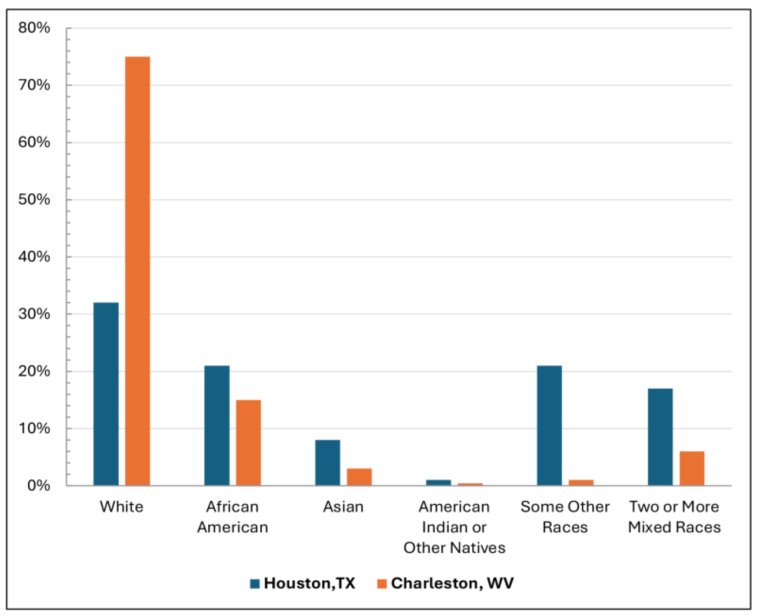
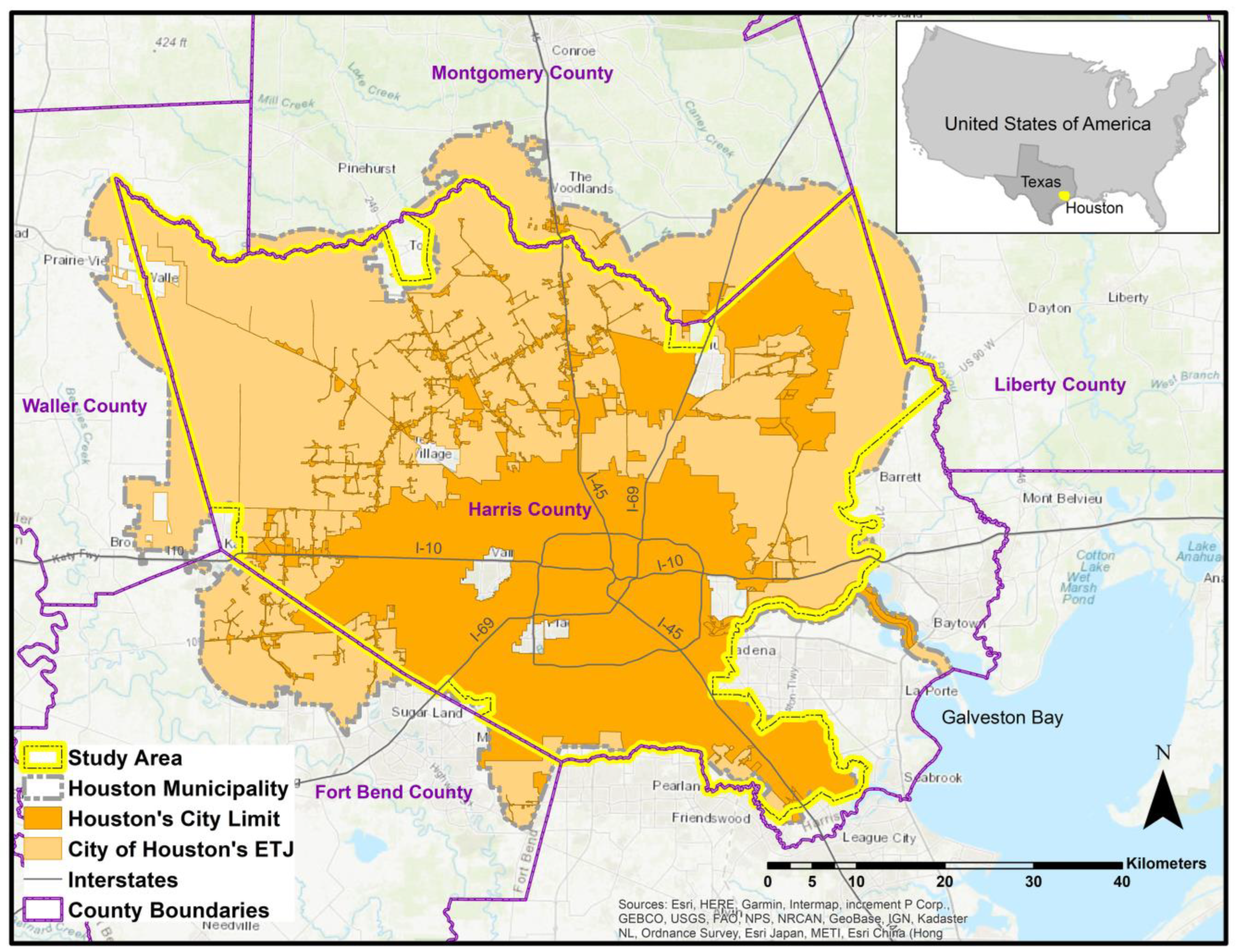
Among the large cities in the United States, Houston is well-known for flooding events affecting the urban area multiple times, from the first years the city was founded in the 1830s to recent decades. Examples included floods due to Tropical Storm Allison in 2001, Hurricane Rita in 2005, Hurricane Ike in 2008, and Hurricane Harvey in 2017 in addition to some other deadly floods in 2015 and 2016. The events caused enormous human and physical losses in the area [13,25]. Houston is located in the southeast part of Texas adjacent to Galveston Bay and approximately 80 km from the Gulf of Mexico. The city lies where interstate highways of I-10, I-45, and I-69 intersect. In terms of race and ethnicity, Houston is one of the most diverse cities nationwide with 32% white population, 21% African Americans, 8% Asians, 1% American Indians or other Natives, 21% of other races, and 17% of two or more mixed races [26]. Regarding topography, it belongs to the Coastal Plain physiographic province; consequently, it has been developed in a flat low-altitude region. The urban area within the city limits covers roughly 1554 km2. The municipality also has some rights and responsibilities in the immediate surrounding metropolitan area called the Extraterritorial Jurisdiction (ETJ). The ETJ is an eight-kilometer buffer around the main city limit except where it intersects with another municipality or jurisdiction [27]. We considered the parts of the city limit and ETJ located in Harris County, with some modifications to match the census tracts at the edges, covering 3838 km2, as the Houston study area (Figure 1). According to the 2019 American Community Survey (ASC), 4,186,149 people reside in the above region [26].

2.1.2. Charleston, WV

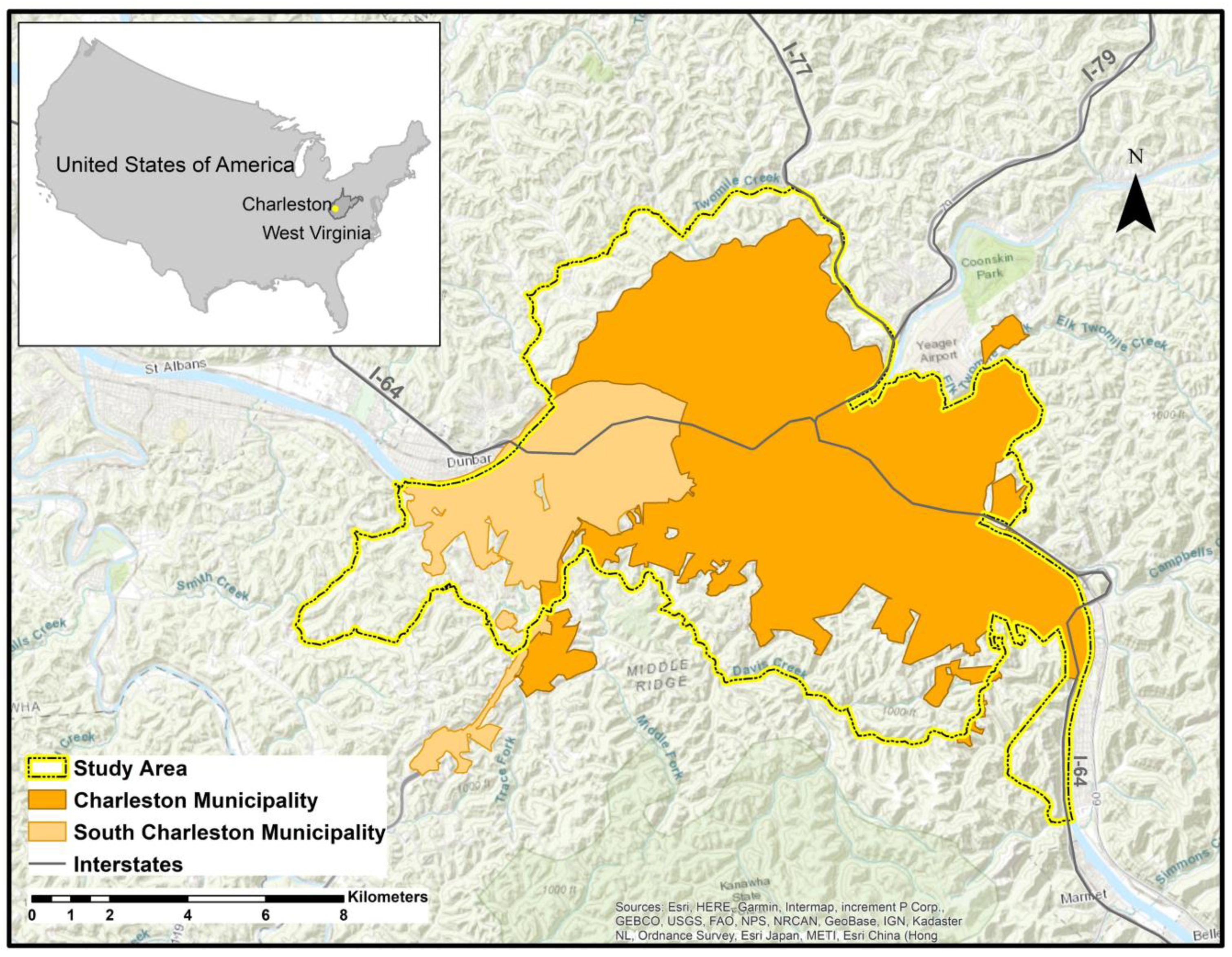
Charleston is the capital city of West Virginia and the largest city in the state. The last severe flood in the city dates back to 2003 [28]; however, with more than three km2 (360 hectares) of developed floodplains, Charleston is at a high risk of flooding [29]. According to the WV Flood Tool created by the West Virginia GIS Technical Center (WVGISTC), about 1700 primary buildings are in the city’s high-risk flood zones [29]. The city is located in the west–central part of Kanawha County at the intersection of interstate highways I-79, I-77, and I-64. Compared to Houston, Charleston has a much lower diversity with 75% white people, 15% African Americans, 3% Asians, less than 1% American Indians or other Natives, 1% of other races, and 6% of two or more mixed races according to the 2020 decennial census [26]. South Charleston is a separate municipality to the west of Charleston. The city covers an area of roughly 22 km2. Its population is 13,647 based on the census results of 2020. In terms of the physiographic provinces, the area belongs to the mountainous region of the Appalachian Plateaus. For definition of the study area, we considered the census tracts that were entirely in the cities in addition to those partially intersecting the above areas, of which most developed areas were within the city limits. We defined an area of 146 km2 as the above study area (Figure 2). The population of the region is 62,840 based on the 2019 ACS [26].
Figure 3 summarizes and compares the racial ratios in the study areas. As shown in the bar chart, Houston is more diverse in terms of race compared to Charleston.

2.2. Data Collection

We used relevant national, state, and local sources to collect the required data to prepare the base maps for further analyses in the study areas. The required GIS floodplain mapped data by FEMA were downloaded for the counties containing the study areas. The website FEMA’s National Flood Hazard Layer (NFHL) Viewer provides access to the database [30]. For the physical exposure analysis, we used the Multi-Resolution Land Characteristics Consortium (MRLC) website to obtain the 30-m National Land Cover Database (NLCD) data of 2019 [31]. For gathering the required demographic data for human exposure, the study referred to the 2019 American Community Survey (ACS) 5-year estimates of the United States Census Bureau [26]. The same data source provided the socioeconomic data for the vulnerability studies in the urban areas.

2.3. Data Analysis

2.3.1. Hazard Base Maps

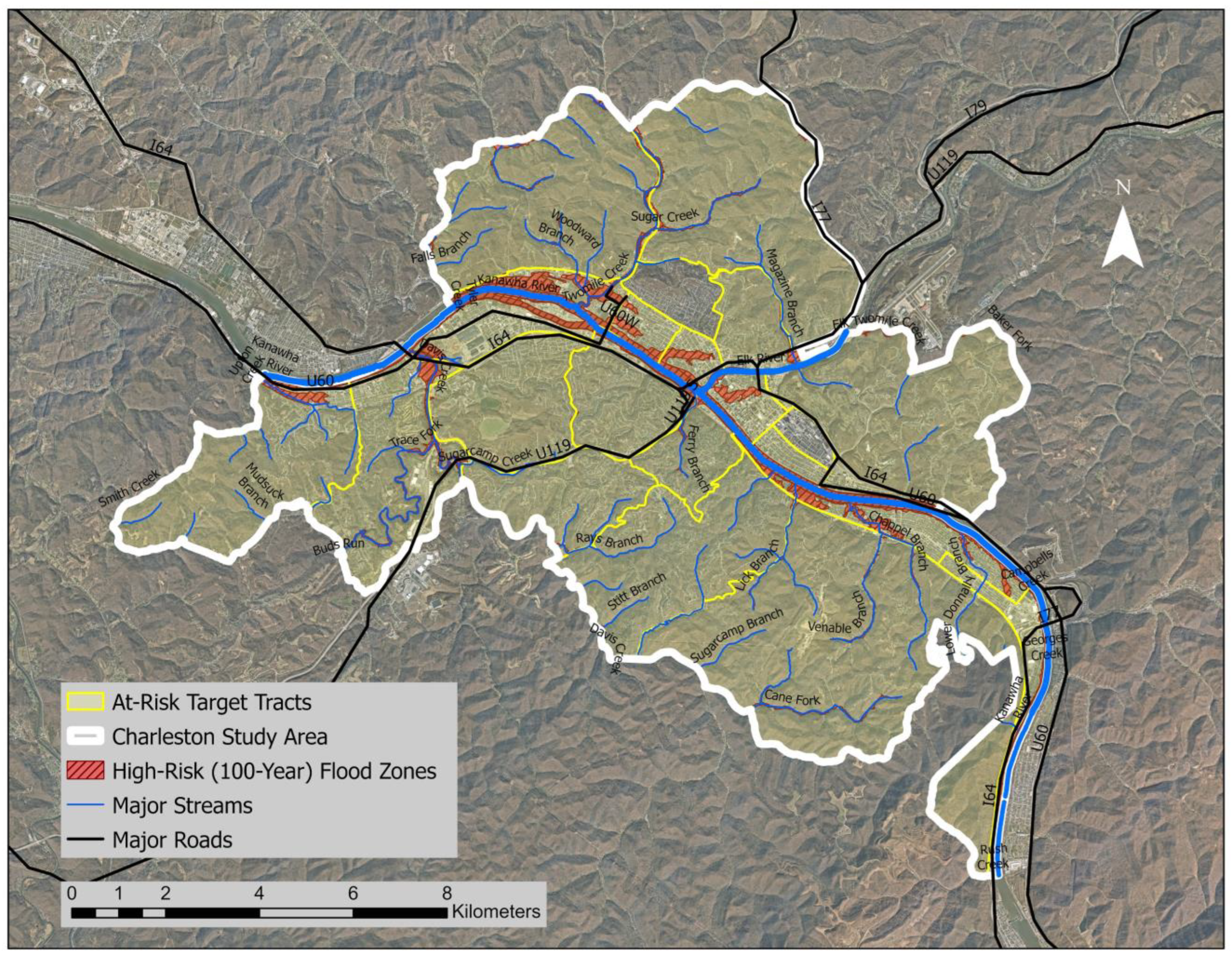
We used ArcGIS Pro Version 3.1 to extract the FEMA’s floodways, 100-, and 500-year floodplains from the NFHL dataset and map them. Floodways are the main channels of streams and their immediately adjacent areas. The 100-year return period floodplains identify the areas of high hazard with the probability of one percent in a given year to be inundated while the 500-year return period zones show the locations of moderate hazard with 0.2 percent of, likelihood in a year. Overlaying the 100-year flood zones and floodways with the census tracts determined the at-risk tracts as the target study units in the study areas. We conducted all of the experiments for those selected tracts.

2.3.2. Exposure Analysis

For the physical exposure, we used the land cover data to estimate the developed area at risk of 100-year flooding in each target census tract. We extracted the total area as the sum of high-, medium-, and low-intensity development categories that intersected with the flood zones. The study excluded the developed open spaces from the analysis of this stage because no primary structures existed in those areas. We analyzed human exposure based on population density in developed areas to estimate the number of people residing in the 100-year flood zones of each census tract. For each target census tract, we calculated the population density in developed areas and then measured the areas of 100-year flood zones. Using the above parameters, the number of people residing in the high-risk flood zones of each tract was estimated by multiplying the density by the flood zone area in developed lands (Equation (1)).
P O P F L = P D D E V × A F L
where POPFL is the estimated population residing in flood zones of the census tract, PDDEV is the population density in developed areas of the census tract, and AFL is the area of 100-year flood zones intersecting the developed land cover categories of the census tract. Furthermore, the study estimated the number of short-term displaced individuals from each tract in case of flooding. The determining factor was the flood depth of 30 cm or deeper which could potentially block the physical access to or from the properties. For that purpose, the depth grid layers for each study area were required. For Charleston, the grid could be accessed via the WVGISTC database [32], while it needed to be produced for Houston using the NFHL dataset based on the methodology described in an online tutorial by FEMA [33]. We investigated the intersection of the inundation areas of the above depth with the developed lands and measured that area for each census tract. With a similar approach to that described earlier, the number of displaced people was estimated by multiplying population density in developed areas by the above inundation area.
Next, we defined a local exposure index for the census tracts in the study areas. A ranking approach similar to the CDC’s Social Vulnerability Index (SVI) described below determined the exposure index scores. First, we ranked the census tracts in each study area from the highest to the lowest values for each factor separately, including the flood-prone population, displaced population, and developed areas in the flood zones. Then, we calculated a percentile rank for each tract based on its position, which was the proportion of the number of tracts below the given one to the total number of target tracts in each city (Equation (2)).
P e r c e n t i l e   R a n k = R a n k 1 N u m b e r   o f   T a r g e t   T r a c t s 1 × 100  
The percentile rank for each factor varying from zero to 100 was the score of the census tract of the indicator for that exposure field. Finally, the total exposure score of each tract was determined as the average of its scores for the three factors. The census tracts with higher scores were identified as those with higher flood exposure in each study area.

2.3.3. Vulnerability Analysis

An essential part of our research examined social vulnerability to floods in the study areas. First, we analyzed the demographic and socioeconomic characteristics that could affect the social vulnerability in Houston and Charleston separately. We considered most of the factors derived from the literature review for which the census data [26] were available in four groups:
  • Socioeconomic status: Under the poverty line, unemployed, employed in industries vulnerable to flooding, and with no high school diploma.
  • Household composition: Age 65 or older, age 14 or younger, single parents, and disabled.
  • Minority status: African-American, Hispanic or Latino, non-citizen, speaking English not fluently.
Housing and Transportation: Residing in mobile homes, inhabiting group quarters, renters, residing in multi-unit (more than 10) apartment buildings, crowded households, and households with no vehicle.
After gathering the data for all the target census tracts, we normalized the above parameters in the form of the percentage of the census tract population.
Our study examined the essential facilities including hospitals, nursing homes, schools, police departments, and fire stations in the flood zones of each tract, as the inundation of such structures can have social consequences making the people residing nearby more vulnerable. Since flood exposure of those facilities can seriously threaten communities, FEMA requires structures to avoid 500-year flood zones or be protected to a higher level if located in those floodplains [34]. For this reason, we mapped those essential facilities in the 500-year flood zones to extract the number of each type of the above essential facilities by census tract. We considered the population growth rate as a factor related to development patterns that could affect social vulnerability. The population of each census tract in 2010 was deducted from that in 2019 to track the changes. Then, the population growth rate was calculated as the proportion of the change in the population in 2010. The percentage of the high-intensity developed land cover class in each tract was another factor to be studied. We used the areas extracted from the exposure study to calculate the percentage of those in each census tract.
Natural disaster vulnerability is highly related to social and physical patterns [12,15,22]. To narrow down the vulnerability factors to the most location-specific parameters, Principal Components Analysis (PCA) programmed in the data analysis software of R (R-4.2.1) was used to determine the significant variation that explained up to 95 percent among the tracts in each urban area. We kept those as the selected factors in each study area for the further steps. The approach was undertaken to note the vulnerability factors that were based on socioeconomic factors in each city instead of applying the same predefined parameters. The next stage was producing a local social vulnerability index for the census tracts in the study areas. We employed the selected parameters from the previous part and applied a similar process as the one described for the exposure index to rank the tracts for each vulnerability factor and give each tract a score. The total vulnerability score was calculated for each tract, averaging the above scores.

2.3.4. Total Risk Analysis

This study stage combined the explained indicators of flood hazard, exposure, and vulnerability in the study areas to introduce the most at-risk communities. The exposure data resulted from overlaying the population and developed lands with the flood zones. Consequently, they already included both exposure and hazard aspects of the risk. The approach integrated the exposure and vulnerability data by combining the indices. The flood risk index was created, averaging each tract’s exposure and vulnerability scores. Accordingly, the final scores were between zero to 100. The tracts with higher scores could be considered as more at-risk of flooding (Equation (3)).
F l o o d   R i s k   S c o r e = E x p o s u r e   S c o r e + V u l n e r a b i l i t y   S c o r e 2  
We applied the relevant methods to analyze the spatial patterns of the produced flood risk index in the study areas. We used the Getis-Ord local statistics within ArcGIS Pro to map the clusters with high values, known as hot spots, at the 95 percent confidence interval. The method produced z-scores and p-values based on each tract in the context of neighboring ones to identify the clusters. Finally, we identified the census tracts in the hot spot areas for which we calculated the mean values of some selected socioeconomic parameters, including unemployment rate, percentages of population below the poverty line, population 25 years or over with no high school diploma, African Americans, Hispanic or Latino, non-citizens, single-parent households, and renter-occupied residential units. The values were compared to the averages for the census tracts in the entire urban area using the t-test in R to see if they significantly differ at the 95 percent confidence interval. Figure 4 functions as a visual summary of the methodology, demonstrating the relationships between the data and various stages of this study. It serves as an aid for articulation of the methodological approach.

3. Results

This section presents the outcomes derived from the analysis of the gathered data in the study areas, shedding light on key observations and significant patterns that emerged during the study.

3.1. Flood Hazard

The hazard analysis showed that there were 882 km2 of high-risk flood zones, including the floodways and 100-year floodplains in the Houston study area (3838 sq km), which could be translated to 23 percent. In the Charleston study area (146 sq km), the high-risk flood zones covered 10 km2 (7%) of the land. According to the created hazard base maps, 547 (78%) of the total 701 census tracts in the Houston study area were known as the at-risk target tracts intersecting the 100-year floodplains (Figure 5). In the Charleston study area, 20 (91%) of the total 22 tracts intersected the 100-year flood zones and were considered as the target tracts for the analyses (Figure 6).

3.2. Flood Exposure

In total, 13 percent (297 sq km) of the developed land in the Houston study area (2245 sq km) was located in the high-risk or 100-year floodplains. Regarding the human exposure, 543,005 people or 13 percent of the population in the above study area (4,186,149) were estimated to reside in the high-risk flood zones. Of the above population, 203,563 persons (5% of the total population) were anticipated to be at risk of short-term displacement caused by floods. The exposure index scores in Houston were in a range between 0.1 and 99.1 of the lowest and highest exposure in the target census tracts, respectively. In the Charleston study area, four km2 or nine percent of the total developed land (43 sq km) were in high-risk flood zones. The estimated population residing in the 100-year floodplains was 5577 or nine percent of the total population of the above study area (62,840). The population that 100-year floods could displace was estimated as 3549 persons (6% of the total population). The exposure scores were between 5.3 and 98.2 in the Charleston study area.

3.3. Social Vulnerability

The Principal Components Analysis (PCA) indicated that 12 of the 20 investigated vulnerability factors could explain more than 95 percent (96.3%) of the variation among the at-risk target tracts in the Houston Study area (Table 2). The vulnerability index was developed based on these selected factors. The index assigned scores between 4.9 to 80.4 to the at-risk census tracts based on their vulnerability level. The median index score in this study area was 45.8. In the Charleston study area, the PCA narrowed down the vulnerability factors to 10 parameters explaining 95.7% of the variability among the census tracts (Table 2). We used those factors to create the vulnerability index for Charleston and obtained scores between 16.3 to 79.5 for the at-risk census tracts.
The detailed results of the Principal Components Analysis (PCA) on 20 vulnerability factors for each study area are presented in the following tables. For Houston, the analysis indicated that 14 principal components could explain 96.3% of the variation among the at-risk target tracts (Table 3). Table 4 displays the matrix of PC1 to PC14 for all 20 vulnerability factors, with the top values (both positive and negative) highlighted. These top values helped identify the 12 most significant social vulnerability variables in this study area.
For Charleston, 10 principal components could explain 95.7% of the variation among the at-risk target tracts (Table 5). Table 6 displays the matrix of PC1 to PC10, with the top values highlighted, which led to the selection of the most significant social vulnerability factors in this study area.

3.4. Flood Risk

The flood risk index combining the exposure and vulnerability indices assigned scores between 8.6 to 86.9 to the target census tracts in the Houston area (Figure 7). With at least 95% of confidence, we could map two urban areas in the north–central and southwest parts as the hot spots of flood risk in the city (Figure 8). Based on our results, those areas are the clusters of census tracts with high, if not necessarily the highest, values of the risk index located near each other.
We could identify 87 census tracts in the risk hot spot areas for which we calculated the mean values of the selected socioeconomic variable. We also computed the averages for the census tracts in the entire urban area to conduct the comparison process. As seen in Table 7, except for the percentage of renter-occupied units, the mean values of the hot spot census tracts for all other investigated factors were significantly higher than those in the study area.
In the Charleston study area, the flood risk index yielded scores between 11.7 and 78.5 (Figure 9). However, our method could not map any significant hot spots for this study area.

4. Discussion

The study results helped to highlight a higher proportion of the 100-year floodplains existed within Houston (23%) than in Charleston (7%) which can be related to the stream network, development pattern, land cover, topography, and other geomorphic characteristics in those urban regions. As mentioned in the study areas description, Houston developed in a flat, low-altitude region, while Charleston is located in a mountainous area. If streams spill over their banks in Houston, they can potentially inundate a larger area due to the region’s flatness. Additionally, the extent and intensity of built environment development are much higher in Houston compared to Charleston, resulting in significantly more areas covered by impervious surfaces in Houston. These factors, along with other detailed geomorphic characteristics, such as soil type, can potentially contribute to larger inundations and a higher floodplain area ratio in Houston. A larger percentage of the developed land area was located within the 100-year flood zones in Houston (13%) compared to Charleston (9%). Consequently, a larger percentage of the population was estimated to reside in the floodplains in Houston (13%) than in Charleston (9%).
We assumed a homogeneous distribution of people in each tract’s developed areas, including the low-, medium-, and high-intensity developed lands, which might be thought of as a limitation. However, it seemed reasonable for the purpose of the research concerning the size of the study areas and data availability. Additionally, we did not assign different weights to the above land cover classes to avoid human bias. However, the non-residential development was kept out of the population estimates model as the above data were combined with the population density of the census tracts. Therefore, low population density in the census tracts with the dominance of non-residential developed areas could control the above effect. Depending on the nature of the data, we created the vulnerability index investigating the demographic and socioeconomic data collected either at the individual or household levels. We preferred the 2019 American Community Survey (ACS) 5-year estimates over the 2020 Decennial Census to keep away the COVID-19 impact on the vulnerability factors. In accordance with the literature [17], we assumed homogenous distribution of those factors within each census tract.
The PCA process removed 8 social vulnerability factors in Houston while taking off 10 in Charleston. The excluded factors were considered less important for the variability in each urban region due to collinearity with the other parameters or not being significantly different among the census tracts. Seven variables related to socioeconomic status, household composition, housing, development pattern, and essential facilities were among the selected principal components in both study areas. However, the other factors were only chosen in one city (Table 2). For example, the percentage of Hispanics or Latinos was one of the principal components in Charleston, not Houston. The reason could be the large population of the above ethnicity distributed in numerous Houston census tracts making them less distinct in this regard. As a general limitation, correlations may still exist among the reduced social vulnerability factors. With more time and resources, future studies can address these relationships and propose solutions for improving the social vulnerability index. In addition, a future research direction could involve investigating more than two urban areas and studying the significant social vulnerability factors that are common across all of them.
While producing the indices, we assumed the same weight for all the indicators to avoid human subjectivity in the model. The decision was consistent with the previous experiments conducted by other authors, such as [15,17]. The final flood risk index combined the exposure and vulnerability indices, averaging their scores. Therefore, a socially vulnerable census tract with only a small area or low population in the floodplain did not get a high score on that index. The disparity between the city limits and census tracts was a limitation while defining the study areas. The tracts did not match the municipality boundaries completely. We decided to include those intersecting the boundaries where most of their developed areas were in the cities. As a result, the modified study areas did not precisely comply with the city limits. With better access to more detailed data, the aerial units can be defined at finer scales, such as census blocks, to make the study areas match the city boundaries better. We investigated the number of essential facilities located in each census tract as a vulnerability factor. However, the scope of services for some of those facilities, such as hospitals, is usually beyond the tract level, which can be a limitation of this approach. In addition, the available data for Houston were limited to the public schools. Therefore, other schools were not included in the model. Access to more comprehensive data on essential facilities and their range of services can result in more accurate vulnerability analyses.
As a general issue of spatial statistics, the study results may be affected by the Modifiable Areal Unit Problem (MAUP). This is defined as the sensitivity of geospatial analysis results to the scale and aggregation type of the data collection units. As a result, the spatial analysis outcomes of a variable depend on the selected scale and size of the study areas [35]. Therefore, replicating the experiments of this study on a different scale than the census tracts may result in different outputs. This problem should be acknowledged and considered for extrapolating to other scales of analysis. While it is impossible to eliminate the MAUP effect, conducting comparable experiments at various scales within the same study area can assist in identifying correlations between the outcomes and allow for the quantification of bias [35].

5. Conclusions

The research supported the defined hypothesis in the Houston study area. The average values of the selected socioeconomic parameters were significantly different, towards vulnerability, in the risk hot spot tracts compared to those in the entire urban area. Thus, with 95% confidence, we could say that there were clusters of high flood risk in Houston where socioeconomically disadvantaged people resided. However, the model could not map any significant flood risk clusters for Charleston. The reason could be the size of the city and its low number of census tracts. The goal of this study was to better understand the spatial pattern of flood risk in two differently sized urban communities and potential correlations to socioeconomic factors. Beyond race and ethnicity, we examined other factors related to social vulnerability to disasters based on the local patterns. The spatial analysis model showed more acceptable performance for mapping risk clusters in large urban areas, like Houston. A need for future studies is to design and test alternative methods for smaller study areas for the identification of significant spatial risk patterns. We applied the 100-year flood zones related to fluvial or riverine flooding published by FEMA as the hazard source. As further steps, more comprehensive hazard maps can be considered, including 500-year zones or different types of floods, such as pluvial or overland flooding. Additionally, the methodology can be combined with future climate change scenarios.
From our literature review searches, we have not been able to find a similar comprehensive study combining the risk elements of hazard, exposure, and social vulnerability in the United States’ urban areas, specifically in Houston, TX or Charleston, WV. Furthermore, no published articles about the spatial distribution of risk in the above regions could be found. Therefore, the study can be considered the first effort in this regard. Moreover, most current disaster vulnerability indices, such as SVI or SoVI, use nationally developed models that apply predefined factors to all study areas. Based on a place-based approach, this study recognized the most significant factors explaining the variations in each urban area and employed those to create the vulnerability and total risk indices for the census tracts in each city. In addition, this article can be considered to contribute toward short-term flood-induced population displacement at the scale of U.S. cities. The detailed result of the evacuation estimates in each census tract can assist city officials and community leaders in devising more appropriate pre-disaster preparation plans. Our methodology limited the population only to developed areas, which can be a more accurate assumption than the other approaches, such as FEMA’s population estimate models [14], which presume homogenous population distribution in each entire census block.
The key parties, such as floodplain managers, urban planners, and policymakers, can use the outcomes of this study for more effective flood risk management. The index scores and other outputs can assist them with a more comprehensive understanding of the most at-risk communities. The risk hot spot areas in Houston should be the priority for flood mitigation actions along with the social justice efforts in this city. This study’s detailed exposure outcomes, including the development and population distribution in floodplains on the tract level, can provide the city, county, and region officials with data to allocate resources, regulations, and plans more efficiently for risk mitigation and resiliency in areas with higher exposure. In addition, more specific results from the study can highlight the areas for urgent mitigation action. For instance, the social vulnerability analysis showed an at-risk census tract in Houston with 99% of the population living in group quarters. The reason was the Harris County Jail located in the floodplain of that tract.
The findings of this study highlight important insights into the flood risk and potential impacts in the studied areas. Despite the discussed limitations, the geospatial analyses combined with the index development techniques enabled a comprehensive location-based assessment of flood exposure, vulnerability, and risk. The approach allowed for identifying significant areas of concern in a large urban area to assist in developing strategies to reduce flood risk and implement effective mitigation measures. Communicating the results of such studies effectively is crucial to ensure the information is understood and utilized by various stakeholders [36]. Clear and concise visual representations, including maps and tables, were used to help with the above purpose. Future efforts to convey results could include public displays on an online interactive tool to be easily accessed by the above groups and the public who want to know more about the risk status at their places of living. Such an online tool can be designed and developed using the output data of this study.
Author Contributions

All authors contributed to the study conception and design. The following summarizes their contributions based on the CRediT taxonomy: Conceptualization, B.B., M.P.S., H.G. and M.S.; Methodology, B.B., M.P.S. and M.S.; Validation, B.B. and M.P.S.; Formal analysis, B.B.; Investigation, B.B.; Resources, B.B. and M.P.S.; Data Curation, B.B. and M.S.; Writing—Original Draft, B.B.; Writing—Review and Editing, M.P.S., H.G. and M.S.; Visualization, B.B.; Supervision, M.P.S.; Project administration, B.B. All authors have read and agreed to the published version of the manuscript.

Funding

This work was supported by the USDA National Institute of Food and Agriculture, Hatch project accession number 7004979, and the West Virginia Agricultural and Forestry Experiment Station.

Data Availability Statement

The raw data can be provided by the corresponding author upon request.

Conflicts of Interest

The authors declare no conflicts of interest.

References

  1. Centre for Research on the Epidemiology of Disasters (CRED) Emergency Events Database (EM-DAT). UCLouvain. 2021. Available online: www.emdat.be (accessed on 17 September 2021).
  2. Crichton, D. UK and global insurance responses to flood hazard. Water Int. 2002, 27, 119–131. [Google Scholar] [CrossRef]
  3. Fedeski, M.; Gwilliam, J. Urban sustainability in the presence of flood and geological hazards: The development of a GIS-based vulnerability and risk assessment methodology. Landsc. Urban Plan. 2007, 83, 50–61. [Google Scholar] [CrossRef]
  4. Koks, E.E.; Jongman, B.; Husby, T.G.; Botzen, W.J.W. Combining hazard, exposure and social vulnerability to provide lessons for flood risk management. Environ. Sci. Policy 2015, 47, 42–52. [Google Scholar] [CrossRef]
  5. Mohanty, M.P.; Simonovic, S.P. Understanding dynamics of population flood exposure in Canada with multiple high-resolution population datasets. Sci. Total Environ. 2021, 759, 143559. [Google Scholar] [CrossRef] [PubMed]
  6. Chakraborty, J.; Collins, T.W.; Montgomery, M.C.; Grineski, S.E. Social and spatial inequities in exposure to flood risk in Miami, Florida. Nat. Hazards Rev. 2014, 15, 04014006. [Google Scholar] [CrossRef]
  7. Qiang, Y. Disparities of population exposed to flood hazards in the United States. J. Environ. Manag. 2019, 232, 295–304. [Google Scholar] [CrossRef] [PubMed]
  8. Tate, E.; Rahman, M.A.; Emrich, C.T.; Sampson, C.C. Flood exposure and social vulnerability in the United States. Nat. Hazards 2021, 106, 435–457. [Google Scholar] [CrossRef]
  9. Kaźmierczak, A.; Cavan, G. Surface water flooding risk to urban communities: Analysis of vulnerability, hazard and exposure. Landsc. Urban Plan. 2011, 103, 185–197. [Google Scholar] [CrossRef]
  10. Kubal, C.; Haase, D.; Meyer, V.; Scheuer, S. Integrated urban flood risk assessment-Adapting a multicriteria approach to a city. Nat. Hazards Earth Syst. 2009, 9, 1881–1895. [Google Scholar] [CrossRef]
  11. Merz, B.; Kreibich, H.; Schwarze, R.; Thieken, A. Review article Assessment of economic flood damage. Nat. Hazards Earth Syst. 2010, 108, 1697–1724. [Google Scholar] [CrossRef]
  12. Birkmann, J. Measuring vulnerability to promote disaster-resilient societies and to enhance adaptation: Discussion of conceptual frameworks and definitions. In Measuring Vulnerability to Natural Hazards: Towards Disaster Resilient Societies, 2nd ed.; Birkmann, J., Ed.; United Nations University Press: New York, NY, USA, 2013; pp. 9–79. [Google Scholar]
  13. Collins, T.W.; Grineski, S.E.; Chakraborty, J. Environmental injustice flood risk: A conceptual model case comparison of metropolitan Miami Houston, USA. Reg. Environ. Chang. 2018, 18, 311–323. [Google Scholar] [CrossRef] [PubMed]
  14. Federal Emergency Management Agency (FEMA). Hazus®-MH Technical Manual: Multi-Hazard Loss Estimation Methodology, Flood Model; Department of Homeland Security: Washington, DC, USA, 2020. Available online: https://www.fema.gov/sites/default/files/2020-09/fema_hazus_flood-model_technical-manual_2.1.pdf (accessed on 7 June 2019).
  15. Cutter, S.L.; Boruff, B.J.; Shirley, W.L. Social vulnerability to environmental hazards. Soc. Sci. Quart. 2003, 84, 242–261. [Google Scholar] [CrossRef]
  16. Tyler, J.; Sadiq, A.A.; Noonan, D.S. A review of the community flood risk management literature in the USA: Lessons for improving community resilience to floods. Nat. Hazards 2019, 96, 1223–1248. [Google Scholar] [CrossRef]
  17. Flanagan, B.E.; Gregory, E.W.; Hallisey, E.J.; Heitgerd, J.L.; Lewis, B. A social vulnerability index for disaster management. J. Homel. Secur. Emerg. 2011, 8, 0000102202154773551792. [Google Scholar] [CrossRef]
  18. Flores, A.B.; Collins, T.W.; Grineski, S.E.; Chakraborty, J. Social vulnerability to Hurricane Harvey: Unmet needs and adverse event experiences in Greater Houston, Texas. Int. J. Disaster Risk Reduct. 2020, 46, 101521. [Google Scholar] [CrossRef]
  19. Morrow, B.H. Identifying and mapping community vulnerability. Disasters 1999, 23, 1–18. [Google Scholar] [CrossRef] [PubMed]
  20. Fernandez, P.; Mourato, S.; Moreira, M.; Pereira, L. A new approach for computing a flood vulnerability index using cluster analysis. Phys. Chem. Earth Parts A/B/C 2016, 94, 47–55. [Google Scholar] [CrossRef]
  21. Röthlisberger, V.; Zischg, A.P.; Keiler, M. Identifying spatial clusters of flood exposure to support decision making in risk management. Sci. Total Environ. 2017, 598, 593–603. [Google Scholar] [CrossRef] [PubMed]
  22. Dewan, A.M. Floods in a Megacity: Geospatial Techniques in Assessing Hazards, Risk and Vulnerability; Springer: Dordrecht, The Netherlands, 2013; Available online: https://link.springer.com/content/pdf/10.1007/978-94-007-5875-9.pdf (accessed on 1 November 2019).
  23. Internal Displacement Monitoring Centre (IDMC). Global Internal Displacement Database: IDMC Query Tool—Disaster. 2022. Available online: https://www.internal-displacement.org/database/displacement-data (accessed on 12 December 2022).
  24. Environment Systems Research Institute (ESRI). ArcGIS Pro Software, Version 3.0; Environment Systems Research Institute (ESRI): Redlands, CA, USA, 2022.
  25. Harris County Flood Control District. Flooded from the Beginning. Harris County’s Flooding History. 2022. Available online: https://www.hcfcd.org/About/Harris-Countys-Flooding-History (accessed on 14 February 2022).
  26. United States Census Bureau. Advanced Search. 2019. Available online: https://data.census.gov/advanced (accessed on 20 May 2022).
  27. City of Houston Annexation. Planning & Development. 2022. Available online: https://www.houstontx.gov/planning/Annexation (accessed on 21 February 2022).
  28. Robinson, D.; Flash Floods of 16 June 2003. Storm Highway. 2003. Available online: https://stormhighway.com/june162003.php (accessed on 14 February 2022).
  29. West Virginia GIS Technical Center (WVGISTC). WV Flood Tool. 2022. Available online: https://mapwv.gov/flood/map/?wkid=102100&x=-9088517&y=4628062&l=5&v=2 (accessed on 9 December 2022).
  30. Federal Emergency Management Agency (FEMA). FEMA’s National Flood Hazard Layer (NFHL) Viewer. 2022. Available online: https://hazards-fema.maps.arcgis.com/apps/webappviewer/index.html?id=8b0adb51996444d4879338b5529aa9cd (accessed on 17 June 2022).
  31. Multi-Resolution Land Characteristics Consortium (MRLC). NLCD 2019 Land Cover (CONUS) Data. 2021. Available online: https://www.mrlc.gov/data?f%5B0%5D=category%3ALand%20Cover&f%5B1%5D=year%3A2019 (accessed on 20 August 2021).
  32. West Virginia GIS Technical Center (WVGISTC). GIS Data. 2019. Available online: https://wvgis.wvu.edu/data/data.php (accessed on 11 March 2019).
  33. Federal Emergency Management Agency (FEMA). Hazus|Create a Depth Grid from DFIRMs. YouTube. 2019. Available online: https://www.youtube.com/watch?v=8CNtSAXoRIk (accessed on 6 July 2022).
  34. Federal Emergency Management Agency (FEMA). Critical Facility. 2020. Available online: https://www.fema.gov/glossary/critical-facility#:~:text=Typical%20critical%20facilities%20include%20hospitals,critical%20records%2C%20and%20similar%20facilities (accessed on 14 February 2022).
  35. Arbia, G. Spatial Data Configuration in Statistical Analysis of Regional Economic and Related Problems; Kluwer Academic Publishers: Dordrecht, The Netherlands, 1989. [Google Scholar]
  36. Percival, S.E.; Gaterell, M.; Hutchinson, D. Effective flood risk visualisation. Nat. Hazards 2020, 104, 375–396. [Google Scholar] [CrossRef]
Figure 1. Houston study area, city limit, and ETJ.
Geohazards 05 00042 g001
Figure 2. Charleston study area.
Geohazards 05 00042 g002
Figure 3. Racial diversity in population of the study areas.
Geohazards 05 00042 g003
Figure 4. Methodology flowchart.
Geohazards 05 00042 g004
Figure 5. At-risk census tracts in the Houston study area.
Geohazards 05 00042 g005
Figure 6. At-risk census tracts in the Charleston study area.
Geohazards 05 00042 g006
Figure 7. Mapped flood risk index in Houston.
Geohazards 05 00042 g007
Figure 8. Flood risk index hot spots in Houston.
Geohazards 05 00042 g008
Figure 9. Mapped flood risk index in Charleston.
Geohazards 05 00042 g009
Table 1. Social vulnerability factors.
Socioeconomic FactorReferences
Economic Status[7,9,13,15,16,17,18,19]
Race/Ethnicity[8,13,15,17,18,19,20]
Age[7,13,15,17,19,20]
Education[15,17,19]
Household Composition[7,9,15,17,19]
Housing Characteristics[15,18,19,20]
Living in Group Quarters[9,17]
Residing in Mobile Homes[8,17,19]
Vehicle Ownership/Access to Transport[17]
Table 2. Selected social vulnerability factors based on PCA in the study areas.
CategoryVulnerability FactorStudy Area of Significance
Minority Status% Black or African-American populationHouston
% Hispanic or LatinoCharleston
% Households with limited English-speaking skillsCharleston
Socioeconomic StatusUnemployment rateHouston and Charleston
% Employed in occupations vulnerable to floodingHouston and Charleston
Household Composition% Single-parent householdsHouston and Charleston
Housing and Transportation% Mobile homesHouston and Charleston
% Renter-occupied residential unitsCharleston
% Multi-unit (10 or more) residential buildingsHouston
% Crowded units (less than one room per person)Houston and Charleston
% Population inhabiting group quartersHouston
% Workers with no vehicleHouston
Development PatternPopulation growth rateHouston
High-intensity developed ratioHouston and Charleston
Essential FacilitiesNumber of essential facilities in the 500-year floodplainsHouston and Charleston
Table 3. Variance percentages of PCA for social vulnerability factors in Houston.
Principal ComponentEigenvalueVariance PercentCumulative Variance Percent
PC16.3331.6731.7%
PC22.7813.8845.5%
PC32.1810.9256.5%
PC41.346.7063.2%
PC51.105.5268.7%
PC61.045.1973.9%
PC70.824.0978.0%
PC80.703.5181.5%
PC90.683.3884.9%
PC100.613.0687.9%
PC110.532.6690.6%
PC120.482.4293.0%
PC130.351.7594.8%
PC140.321.5896.3%
PC150.211.0797.4%
PC160.170.8798.3%
PC170.140.6899.0%
PC180.090.4599.4%
PC190.060.3099.7%
PC200.060.28100.0%
Table 4. PC1 to PC14 matrix for social vulnerability factors in Houston.
Vulnerability FactorPC1PC2PC3PC4PC5PC6PC7PC8PC9PC10PC11PC12PC13PC14
% Black or African-American population0.050.310.44−0.140.29−0.01−0.030.03−0.05−0.04−0.11−0.30−0.350.50
Unemployment rate0.100.090.48−0.020.100.08−0.25−0.37−0.11−0.190.590.120.30−0.09
% Employed in occupations vulnerable to flooding0.35−0.150.12−0.010.09−0.06−0.07−0.030.12−0.05−0.11−0.13−0.190.11
% Single-parent households0.220.100.22−0.340.120.010.000.600.04−0.28−0.170.060.13−0.37
% Mobile homes0.09−0.300.00−0.040.290.100.690.08−0.450.060.28−0.07−0.09−0.05
% Multi-unit (10 or more) residential buildings0.140.45−0.24−0.13−0.11−0.100.180.050.110.090.200.290.010.10
% Crowded units (less than one room per person)0.32−0.09−0.03−0.070.000.02−0.09−0.200.080.150.120.22−0.67−0.31
% Population inhabiting group quarters−0.010.13−0.130.330.700.17−0.270.11−0.110.34−0.130.310.09−0.03
% Workers with no vehicle0.230.250.01−0.03−0.18−0.03−0.170.00−0.310.53−0.01−0.540.11−0.35
Population growth rate−0.080.01−0.08−0.630.32−0.060.16−0.520.130.11−0.32−0.010.22−0.11
High-intensity developed ratio0.160.23−0.220.06−0.130.23−0.08−0.26−0.60−0.48−0.340.10−0.070.00
Number of essential facilities in the 500-year floodplains0.030.05−0.05−0.08−0.080.920.070.020.300.030.05−0.150.000.01
% Households with limited English-speaking skills0.33−0.19−0.140.04−0.04−0.020.020.05−0.030.09−0.06−0.100.310.39
% Non-citizen0.33−0.05−0.25−0.06−0.06−0.01−0.04−0.110.080.080.160.000.070.29
% Vulnerable ages (65 or older and 14 or younger)−0.01−0.280.30−0.33−0.320.14−0.160.12−0.290.37−0.160.470.000.21
% Renter-occupied residential units0.250.40−0.11−0.090.00−0.100.150.080.070.030.110.17−0.050.09
% Age 16 or older with no high school diploma0.35−0.210.070.110.100.00−0.07−0.040.09−0.05−0.11−0.030.070.06
% Below the poverty line0.330.110.180.11−0.050.020.210.010.000.03−0.070.180.30−0.04
% Population with a disability0.020.150.400.42−0.170.010.41−0.240.180.16−0.350.120.01−0.11
% Hispanic or Latino0.31−0.27−0.070.080.06−0.07−0.09−0.070.18−0.17−0.11−0.010.07−0.21
Table 5. Variance percentages of PCA for social vulnerability factors in Charleston.
Principal ComponentEigenvalueVariance PercentCumulative Variance Percent
PC16.9934.9535.0%
PC23.4117.0752.0%
PC31.919.5361.6%
PC41.708.5170.1%
PC51.507.5177.6%
PC61.206.0083.6%
PC70.733.6787.2%
PC80.683.4190.7%
PC90.572.8693.5%
PC100.442.1895.7%
PC110.261.3297.0%
PC120.221.1198.1%
PC130.150.7698.9%
PC140.090.4399.3%
PC150.060.2999.6%
PC160.040.2199.8%
PC170.030.1399.9%
PC180.010.05100.0%
PC190.000.02100.0%
PC200.000.00100.0%
Table 6. PC1 to PC10 matrix for social vulnerability factors in Charleston.
Vulnerability FactorPC1PC2PC3PC4PC5PC6PC7PC8PC9PC10
% Hispanic or Latino0.160.170.30−0.37−0.200.020.410.05−0.15−0.41
% Households with limited English-speaking skills−0.030.060.120.370.11−0.68−0.160.36−0.09−0.04
Unemployment rate0.29−0.04−0.180.13−0.03−0.080.250.000.580.17
% Employed in occupations vulnerable to flooding0.18−0.25−0.04−0.310.26−0.350.15−0.420.080.01
% Single-parent households0.04−0.340.210.45−0.03−0.130.26−0.08−0.24−0.18
% Mobile homes0.00−0.170.04−0.10−0.73−0.140.040.180.140.06
% Renter-occupied residential units0.340.010.150.020.180.03−0.020.18−0.200.03
% Crowded units (less than one room per person)0.180.14−0.55−0.05−0.04−0.08−0.10−0.04−0.10−0.40
High-intensity developed ratio0.270.140.020.130.140.09−0.360.120.43−0.42
Number of essential facilities in the 500-year floodplains0.170.410.160.03−0.07−0.06−0.13−0.33−0.15−0.23
% Non-citizen0.100.390.29−0.06−0.03−0.26−0.14−0.32−0.010.33
% Population inhabiting group quarters0.170.34−0.060.26−0.37−0.010.05−0.130.110.23
% Workers with no vehicle0.27−0.220.260.02−0.050.23−0.35−0.11−0.120.22
% Population with a disability0.30−0.20−0.14−0.01−0.040.17−0.240.01−0.140.17
Population growth rate−0.220.18−0.350.240.120.060.21−0.29−0.140.16
% Multi-unit (10 or more) residential buildings0.260.24−0.170.15−0.010.230.170.31−0.370.14
% Age 16 or older with no high school diploma0.23−0.23−0.27−0.20−0.11−0.27−0.24−0.06−0.270.05
% Below the poverty line0.33−0.10−0.170.11−0.09−0.150.25−0.07−0.06−0.01
% Black or African-American population0.23−0.190.190.350.060.210.16−0.250.09−0.13
% Vulnerable ages (65 or older and 14 or younger)−0.25−0.13−0.070.23−0.330.06−0.28−0.34−0.09−0.28
Table 7. Results of comparing socioeconomic factors in hot spot tracts and the Houston study area.
Socioeconomic FactorMean in Risk Hot Spot Census TractsMean of All Census Tracts in Study Areat-Test for Mean Difference (95% CI)
% Population with No High School Diploma34.3%20.4%Significant, p-value = 2.723 × 10⁻¹⁶
% Population Below Poverty Level26.1%17.7%Significant, p-value = 2.143 × 10⁻¹⁰
% Hispanic or Latino59.9%42.5%Significant, p-value = 6.005 × 10⁻¹¹
% Single-Parent Households12.8%8.9%Significant, p-value = 5.651 × 10⁻⁶
% Black or African-American31.4%20.2%Significant, p-value = 1.217 × 10⁻⁵
% Population with a Disability11.0%9.5%Significant, p-value = 0.007343
Unemployment Rate6.7%5.8%Significant, p-value = 0.01883
% Non-US Citizens19.7%17.5%Significant, p-value = 0.02437
% Renter-Occupied Residential Units48.0%46.7%Not Significant, p-value = 0.3054
Disclaimer/Publisher’s Note: The statements, opinions and data contained in all publications are solely those of the individual author(s) and contributor(s) and not of MDPI and/or the editor(s). MDPI and/or the editor(s) disclaim responsibility for any injury to people or property resulting from any ideas, methods, instructions or products referred to in the content.