Article

Investigation of Tsunami Waves in a Wave Flume: Experiment, Theory, Numerical Modeling

by
Boris Vladimirovich Boshenyatov
Institute of Applied Mechanics of Russian Academy of Sciences, 125040 Moscow, Russia
GeoHazards 2022, 3(1), 125-143; https://doi.org/10.3390/geohazards3010007
Submission received: 21 December 2021 / Revised: 22 February 2022 / Accepted: 25 February 2022 / Published: 3 March 2022
(This article belongs to the Topic Natural Hazards and Disaster Risks Reduction)

Abstract

:
To protect the coastal areas of the seas and oceans from the destructive force of tsunami waves, coastal and surface barriers are usually built. However, for high waves, these barriers turn into underwater barriers through which tsunami waves pass practically without losing their energy. In this paper, we study a new principle of suppression of the energy of tsunami waves by underwater barriers. The problems of experimental and numerical modeling of the processes of generation, propagation, and interaction of gravity wave of the tsunami type with underwater barriers are considered. It is shown that, under certain conditions near the underwater barriers, large-scale vortex structures occur that accumulate a significant part of the energy of the incident wave. Here, if the barriers parameter h/(H + A) = 0.84 ÷ 0.85 (h—height of the barriers, A—amplitude of incident wave on a barrier, H—depth of the reservoir), then the vortex structures accumulate up to 50% of the wave energy incident on the barrier. A theoretical model explaining the effect of anomalous vortex suppression of tsunami wave energy by underwater barriers has been developed. Theoretical calculations and results of numerical modeling based on the Navier–Stokes Equations are consistent with experimental studies in a hydrodynamic wave flume.

1. Introduction

It is well known that tsunami waves are one of the most dangerous and destructive disasters to which the coastal zone is exposed. The causes of tsunami origination are practically unpredictable factors like earthquakes, landslides, volcanoes, etc. [1]. Far from the coast, these waves are not dangerous because their height rarely exceeds 1 m. However, their wavelength is almost a hundred times greater than the depth of the ocean. Thus propagating in the ocean, as in a basin with a relatively small depth, tsunami wave sets in motion the entire water thickness from the seafloor to surface. That is why these waves transfer a vast amount of energy through great distances, with the speed of an airliner. The advanced speed of tsunami waves in the ocean is quite accurately described by the linear theory of shallow water. If the average depth of the ocean is H = 4000 m, then the tsunami wave speed is с = g H 200   m / s , where g = 9.81 m/s2 is the acceleration of gravity. Upon entry to the zone of shallow water, the front speed of the wave decreases sharply, and the wave height increases tens of times. Inside bays and outfalls, the amplitude of the tsunami wave increases up to 20 m or higher because of space restriction from the sides. The danger of tsunami waves is associated primarily with their unpredictable, sudden, and tremendous energy. Exploring tsunami waves in natural conditions is almost impossible. Experiments in ground facilities usually have a high cost since bringing the wave simulation parameters to natural conditions requires the creation of large-scale (up to 300 m or more) and costly facilities. Therefore, the study of tsunami waves makes extensive use of analytical methods of research, as well as numerical (computer) modeling approaches [1,2,3].
Different barriers are used to protect coastal settlements and industrial facilities: dams located in the sea at a depth of 10–15 m, which rise above the water level up to 4–10 m (offshore tsunami barriers), coastal tsunami barriers, and inland tsunami barriers. The height of such barrier is calculated from the condition of total reflection of the most probable incident wave. [3]. However, if the wave height is greater than half the height of the barrier, which is located above the water, then the barrier is completely under water, and its reflectivity sharply decreases [1,4]. Therefore, studies on increasing the efficiency of underwater barriers are always relevant and continue a wide front [4,5,6,7]. In particular, [4] shows the results of experimental studies on underwater permeable barriers whose destructive power of the waves can be reduced not only by the reflection of the wave but also due to the energy dissipation in the water infiltration through the barrier. It is shown that an impermeable barrier whose height reaches the initial water level decreases the magnitude of the tsunami wave run up by only 37%, whereas an identical permeable barrier does so by 43%. A remarkable exception is the work of [5], in which the effect of anomalously high absorption of energy of tsunami-type waves by two underwater barriers installed at some optimal distance comparable to the depth of water was experimentally discovered. This effect still has no theoretical explanation. Our research [8,9] not only experimentally confirmed the existence of this anomalous effect (including on single barriers) but also explained its physical nature and mechanism.
This paper presents the results of detailed studies of the effects of anomalous suppression of the energy of tsunami waves by single underwater barriers on the basis of physical and numerical modeling of wave processes in the laboratory Нydrodynamic Channel (wave flume) of the Institute of Applied Mechanics of the Russian Academy of Sciences.

2. Problems of Modeling Tsunami Waves in Experimental Facilities

The main cause of the most destructive tsunami waves is underwater earthquakes. They typically evolve from the deep ocean as extremely long waves with small steepness. By nature, the tsunami consists of a number of nonperiodic waves, and during the propagation from the ocean to the nearshore area, these waves gradually modify with respect to amplitudes and wave periods. The main amplification of the amplitude and velocity of the flow occurs at the last stages when interacting with the shelf zone and shallow water. Typical fault areas of major earthquakes are the width 200 km to 300 km and lengths 500 km to 1600 km.
Madsen et al. [7], the parameters of the expected tsunami waves are calculated for the most realistic case of vertical displacement of the water surface due to an underwater earthquake by 2 m on a surface area having a diameter of 400 km. The paper by reference [7] presents data on tsunami wave measurements in the coastal zone of Thailand (depth 14 m) from the Sumatra earthquake of 2004, with a fault width of 200 km and fault length of up to 1600 km. It was shown that an initial wave trough of −2.7 m followed by a wave crest of +3.9 m, i.e., a wave height of 6.6 m. The second trough was only −0.5 m, followed by a crest of 1.7 m, while the third trough was −0.6 m, followed by a crest of +4.9 m. The time span between successive crests or troughs was approximately 13–14 min during the registration. The results of these experiments are consistent with the data in Table 1.
Thus, the actual tsunami waves are more like a rectangular undular bore than a single soliton-type wave, which is often used to simulate tsunami waves in experimental installations and numerical calculations. Note that in studies based on detailed calculations [7,10], it was shown that such a simulation of a tsunami wave by a single soliton wave does not correspond to real conditions and often leads to an underestimation of the destructive power of tsunami waves. In the most general form, the propagation of tsunami waves in the ocean (or in a wave flume) is described by the Navier–Stokes Equations for an incompressible fluid. After reducing these equations to a dimensionless one, we can obtain the following dimensionless similarity criteria:
A H ;     H L ;     c g H ;     g H L t ;     r H ;     ρ η A g H
where t is time, r is a distance, and ϱ and η are density and coefficient of dynamic viscosity, respectively. In accordance with the law of similarity, the physical model accurately describes the natural phenomena if all the dimensionless parameters (1) have the same value in the model and in nature. To achieve such a simulation in real conditions is not possible. In order to approximate simulation conditions to full-scale ones (Table 1), even for the first two, the most important parameters, it is necessary to build large-scale and expensive installations and structures [11] or significantly improve the accuracy of measuring wave parameters [12]. In addition, in order to adequately transfer the results of experiments in hydrodynamic installations to natural conditions, it is necessary to study in detail the laws of similarity to reveal areas of self-similarity when the dependence on the value of a particular criterion disappears.

3. Mathematic Model and Numerical Method

We consider the unsteady flow of an incompressible viscous fluid with a free surface in a channel of a variable cross section. Reynolds numbers for the flows of liquid in the hydrodynamic channel can reach the values of the order of 104; however, in our calculations of the turbulence model, they are omitted. The reason for this approach is the fact that the experiments in rectangular channels [13] show high enough Reynolds numbers of transition to the turbulent state R e * = ρ U H η , where U is a fluid velocity. At that, the value Re* increases with decreasing of the distance from the channel entrance.
Thus, at x/H = 60, the beginning of the transition into the turbulent state corresponds to Re1* = 8 × 10³ and the end of the transition to Re2* = 1.8 × 10⁴. Furthermore, it is known that when the initial perturbation in the flow decreases, the Reynolds of the transition increases as well. In this case (at the wave length of L ≈ 3 m, H ≈ 0.1 m), the value x/H ≤ 30, and the initial perturbations before the wave are close to zero.
Thus, the flow of liquid in the channel is described by Navier–Stokes Equations (2) and (3), which are solved by the numerical method of finite volumes, with a use VOF (Volume of Fluid) method [14] along with the Equation (4) of the scalar value γ conservation:
U = 0
( ρ U ) t + U ( ρ U ) = p + η 2 U + ρ g ρ F σ
γ t + ( U γ ) = 0
where p is pressure, γ is the volume concentration of the carrier fluid in the computational cell. The value of the scalar function γ in the cell can indicate one of the three states: γ = 0—the cell contains air only; γ = 1—the cell contains water only; 0 < γ < 1—the cell contains an interface between liquid and gas. Thus, in this case, γ is an indicator of interfacial surfaces and free liquid surfaces. Physical properties of the medium are calculated as weighted averages in accordance with the volume concentration of phases in each cell. The average density in the cell is calculated as ρ = γρ1+ (1 − γ) ρ2, where ρ1—density of the carrier fluid, ρ2—density of air; accordingly, the viscosity: η = γη1 + (1 − γ)η2. The force caused by surface tension F σ = σ k γ , where σ = 72.8 N/m is the surface tension of water–air; k = ( γ | γ | ) = n .
The computational area, according to the initial state of the water levels in the channel and in the caisson generator (see Section 5.1), includes two subareas: the lower subarea is filled with water that has a preset initial configuration of the interface; the upper one—with air. In the computational area, different obstacles (mobile and fixed), submerged breakwaters, etc., can be placed. At t = 0 under the influence of gravity, a wave motion is generated, which should be calculated. The boundary conditions on the rigid walls of the channel (and the walls of the rigid obstacles) are set as follows:
U = 0 ,   n γ = 0
On the free surface of the liquid y = h(x,t) = H + ξ (x,t), where ξ (x,t) is the displacement of the free surface, the kinematic and dynamic conditions are met in the traditional formulation: h t + u x h t = u y and pnn = −patm, pns = 0; where pnn, pns are normal and tangential stresses, patm is external pressure.
The initial condition at t = 0: at 0 x 1.5   m the distribution function h(x,0) = H + A; at 1.5   m x 15   m the distribution function h(x,0) = H.
Numerical calculations were carried out using the InterFoam solver of the free software package OpenFOAM [15].

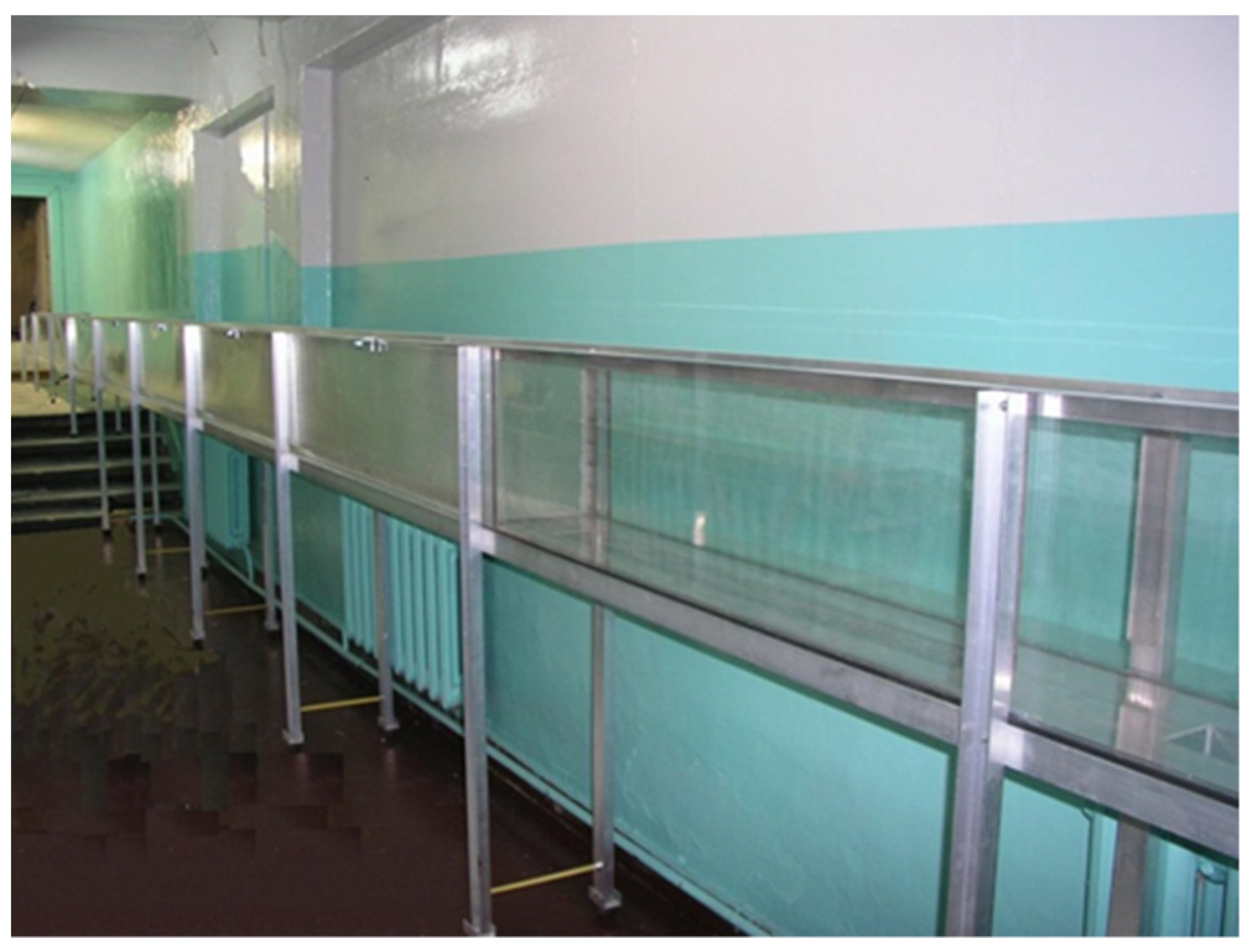
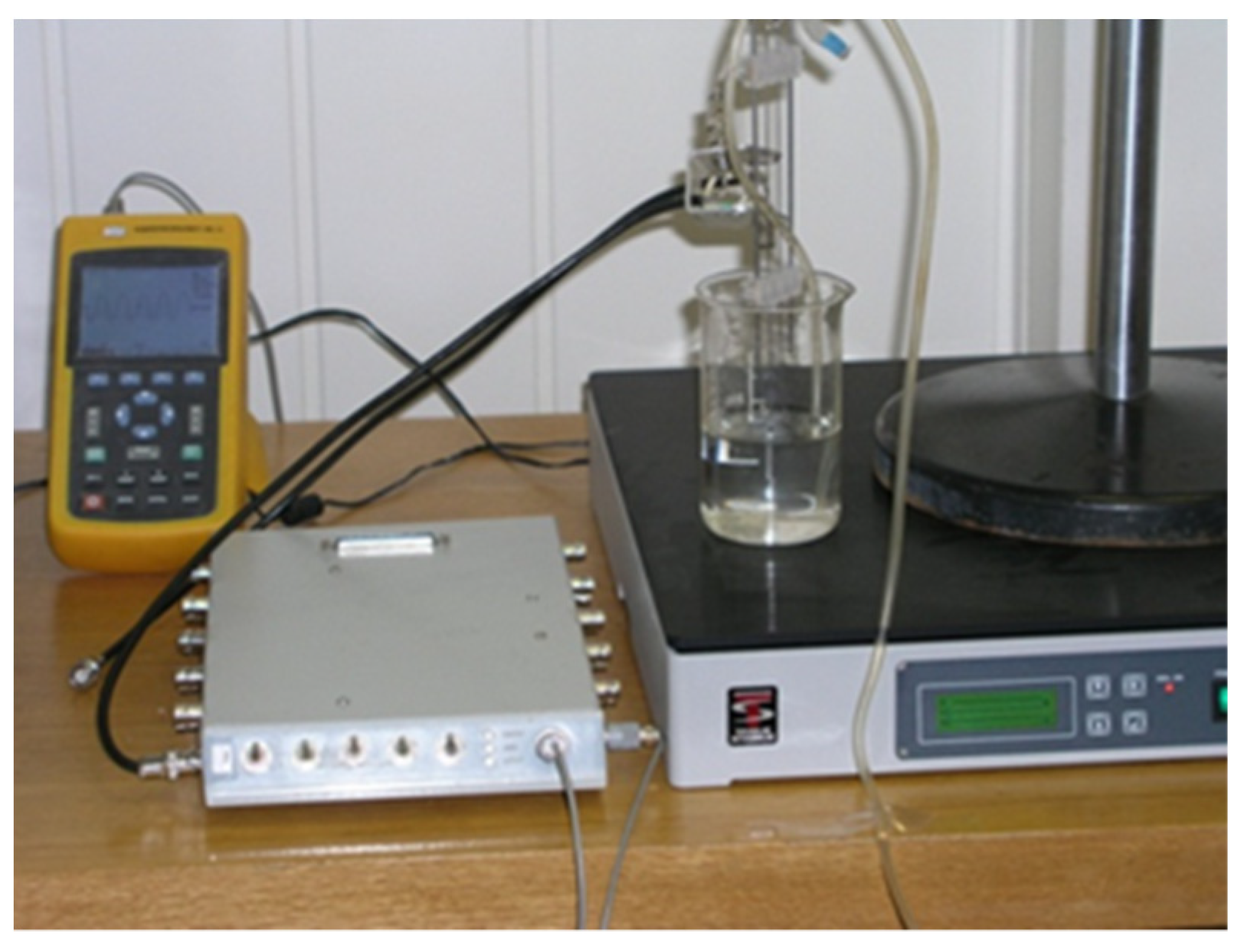
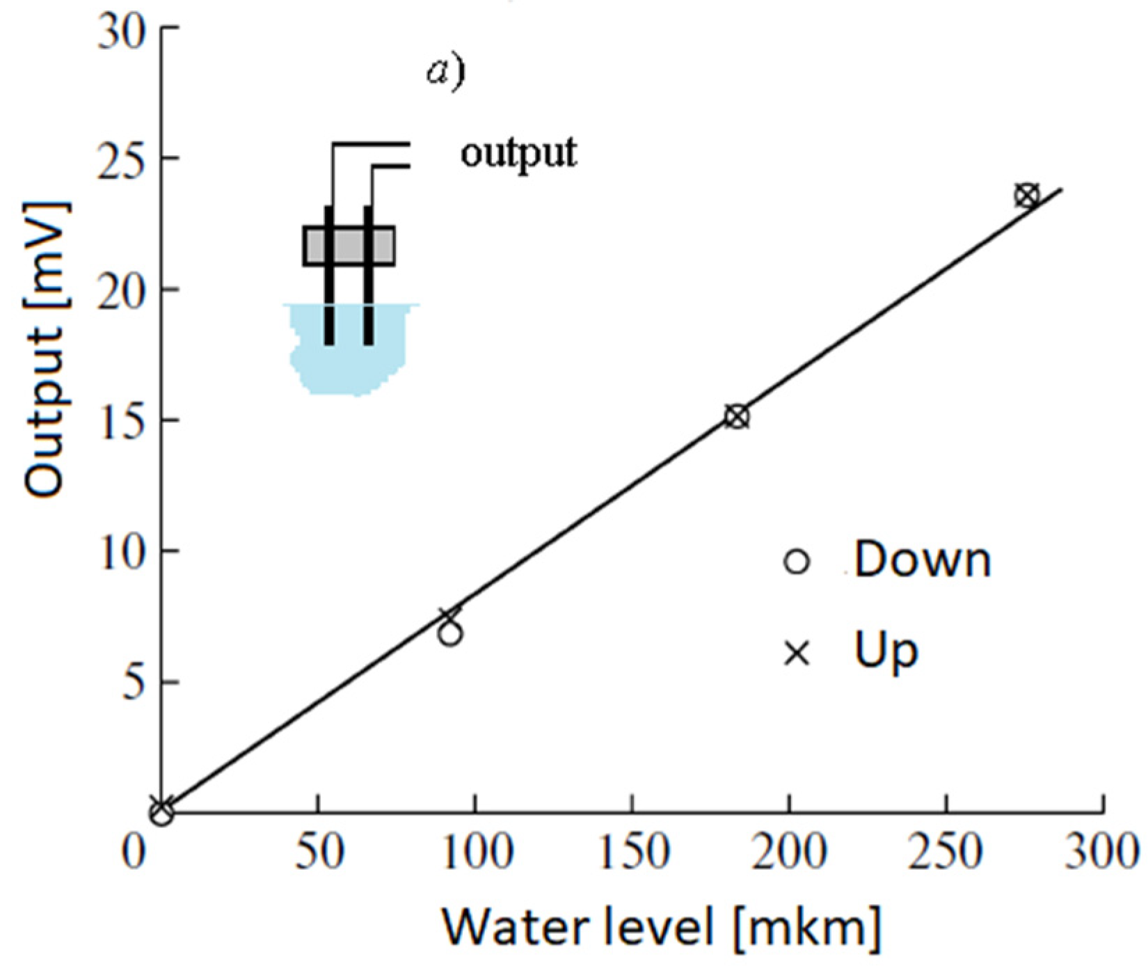
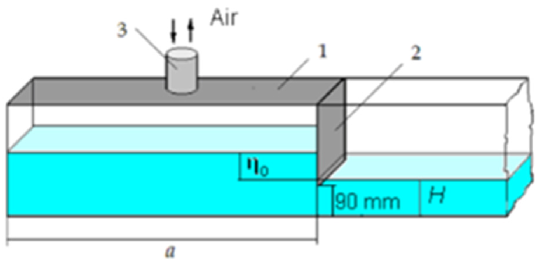
4. Experimental Equipment and Research Methods

Hydrodynamic channel of the Institute of Applied Mechanics of Russia Academy of Science (IPRIM RAS) has the following dimensions: length—15 m, width—0.26 m, height—0.35 m (see Figure 1).
The author of this work showed in Reference [10] that the use of high-precision wave amplitude measurement methods [12] combined with numerical modeling [16] allows the simulation and investigation of many tsunamis wave problems in relatively small-sized laboratory facilities.
Experiments and numerical simulation of wave processes were carried out in the channel using the following parameters:
  • Initial water depth in channel H varied from 100 mm to 103 mm;
  • Wave length L ≈ 3 m, averaged incident wave amplitude A in a series of experiments ranged from 0.5 mm to 15 mm.
Thus, in our setup, we simulate the dimensionless parameters of tsunami waves close to the parameters of Table 1: 0.005 < A/H < 0.15 and H/L ≈ 0.03.
Resistive sensors of water level, ten-channel measuring apparatuses [16,17], four-channel digital oscilloscope, and a two-channel recorder Velleman PCS 500 were used for registering wave processes in the channel. The water level sensor consists of two insulated needles, the resistance between which, when immersed in water, is proportional to the depth of immersion. Figure 2 shows equipment for precision calibration of resistive sensors intended for measuring the water level. A tripod with a sensor and a cuvette with water are placed on the vibration protection platform. Figure 3 shows a typical calibration graph of the measurement channel. It can be seen that the error in measuring the water level does not exceed 10 microns.
Resistive sensors, which were located at various distances from the wave generator, measured the displacement of the free surface of the water at the time intervals ξ(t). It is now possible to draw wave x-t diagrams for each experiment and to determine: the velocity of waves and the amplitude factors of wave reflection R = W r W A r A and of wave transition T = W t W A t A during the interaction with the underwater barriers. Here W; Wr and Wt are the total energy of the incident, reflected, and transmitted waves, respectively. Ar and At are averaged amplitudes of reflected and transmitted waves.
The wave flume is equipped with a high-speed digital video camera Photron FASTCAM SA4500K, with a shooting speed of up to 3600 frames/s at full resolution 1024 × 1024.

5. Generation and Propagation of Waves in a Wave Flume

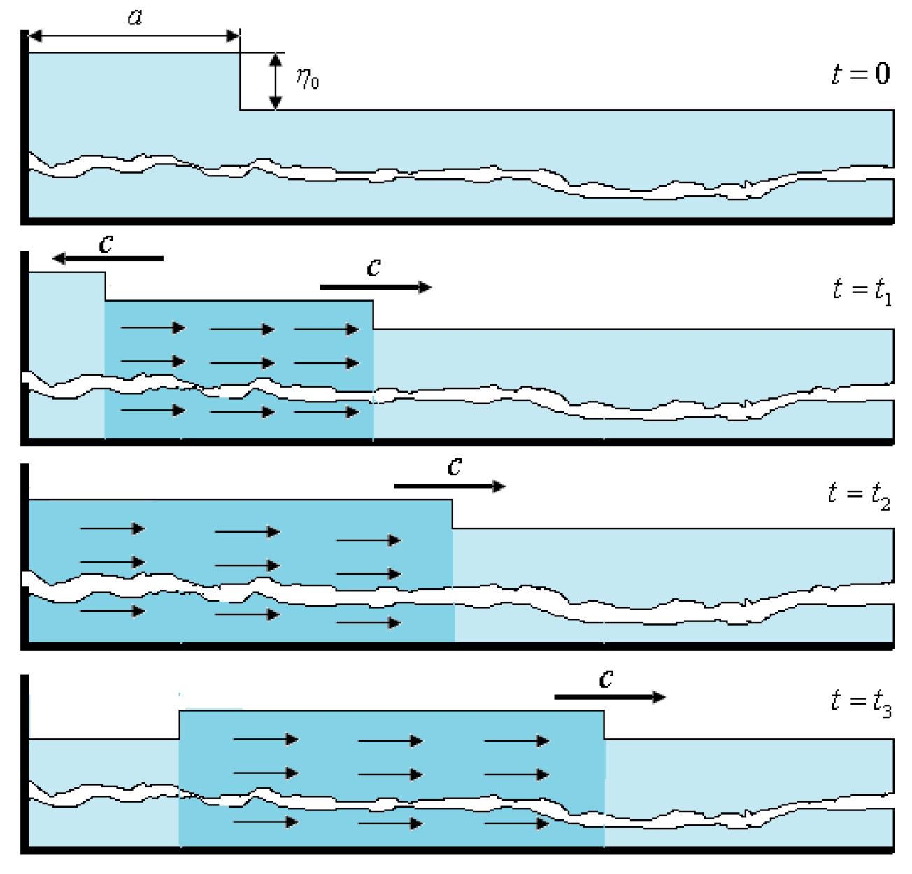
5.1. Wave Initiation

Unlike the common method of initiating waves with the use of various moving mechanisms, such as vertical movement of the bottom or movement of the angled wall of wave generator [1,5,11], the wave generator in the IPRIM RAS hydrodynamic channel has no moving parts. The method of gravity waves initiation is based on the breakdown of an arbitrary discontinuity of water levels in the channel and in the wave generator, which is set in the initial time. This method is technically implemented in the caisson-type wave generator (Figure 4), which is a compartment of the channel (length a = 1465 mm) with the sealed top cover (1) and front wall (2) submerged during operation.
In the top cover of the wave generator, there is a tube (3) provided for pumping out and filling with the air the upper volume of the generator, while the 90 mm high lower part of the generator communicates with the effective volume of the channel. Before the operation, the channel is filled with water up to the level of H0 > 90 mm. Then, the air is evacuated via tube (3) from the upper part of the generator, thereby attaining specified water level difference η0: the water level (H + η0) in the generator and the water level H in the working part of the channel. After depressurization (t = 0) of the upper part of the generator, the wave is initiated in the working part of the channel. The wave has the length L ≈ 2a and the amplitude Аη0/2 (see Appendix A).
Let us refer to the wave generator, which at the time t = 0 instantly retracts the front wall, as an ideal one. The work of the ideal generator and the real (caisson-type) one was compared using numerical simulation. At a distance x > a from the front wall of the generator, calculated profiles of gravity wave ξ(t) of the ideal generator and the caisson-type one were almost identical.
The process of tsunami-type wave generation in the hydrodynamic channel (wave flume) of the IPRIM RAS is shown in Figure 5. At the initial moment of time t = 0, the process of decay of a given level difference δ0 = 2A is started. Up to this point in time, the water in the generator and the working channel was at rest. At t = 0.7 s, we see that the initial level difference split into two waves: a negative wave (−A) moves inside the generator (a = 1.465 m), a wave with a height (+A) moves into the working part of the hydrodynamic channel. In each image, above the white horizontal line, we can see the profiles of the water levels in these waves, below the longitudinal velocity. Further, at t = 2 s and t = 3.3 s, we see that the wave (−A) reflected from the generator wall and formed a single wave with height (+A) and length L = 2a, which moves into the working part of the wave flume. The wave speed is c = g H = 1   m / s . The velocity of liquid in the channel before and after the wave was zero.
Note that the shape of the generated wave (with damped oscillations) is very similar to the shape of a natural tsunami wave, which is formed because of an underwater earthquake [5].
Figure 6 shows a comparison of experimental oscillogram of wave height versus time ξ(t), based on measurements taken by the level sensor at a distance of 1.5 m from the front wall of wave generator, with calculated dependence for ideal generator (black line) at the same initial conditions: H = 0.102 m; η0 = 0.015 m.
We can see that at a distance of x = aL/2, the experimental dependence is practically the same as the calculated dependence for the ideal generator; further on (at x > a), the coincidence is closer.

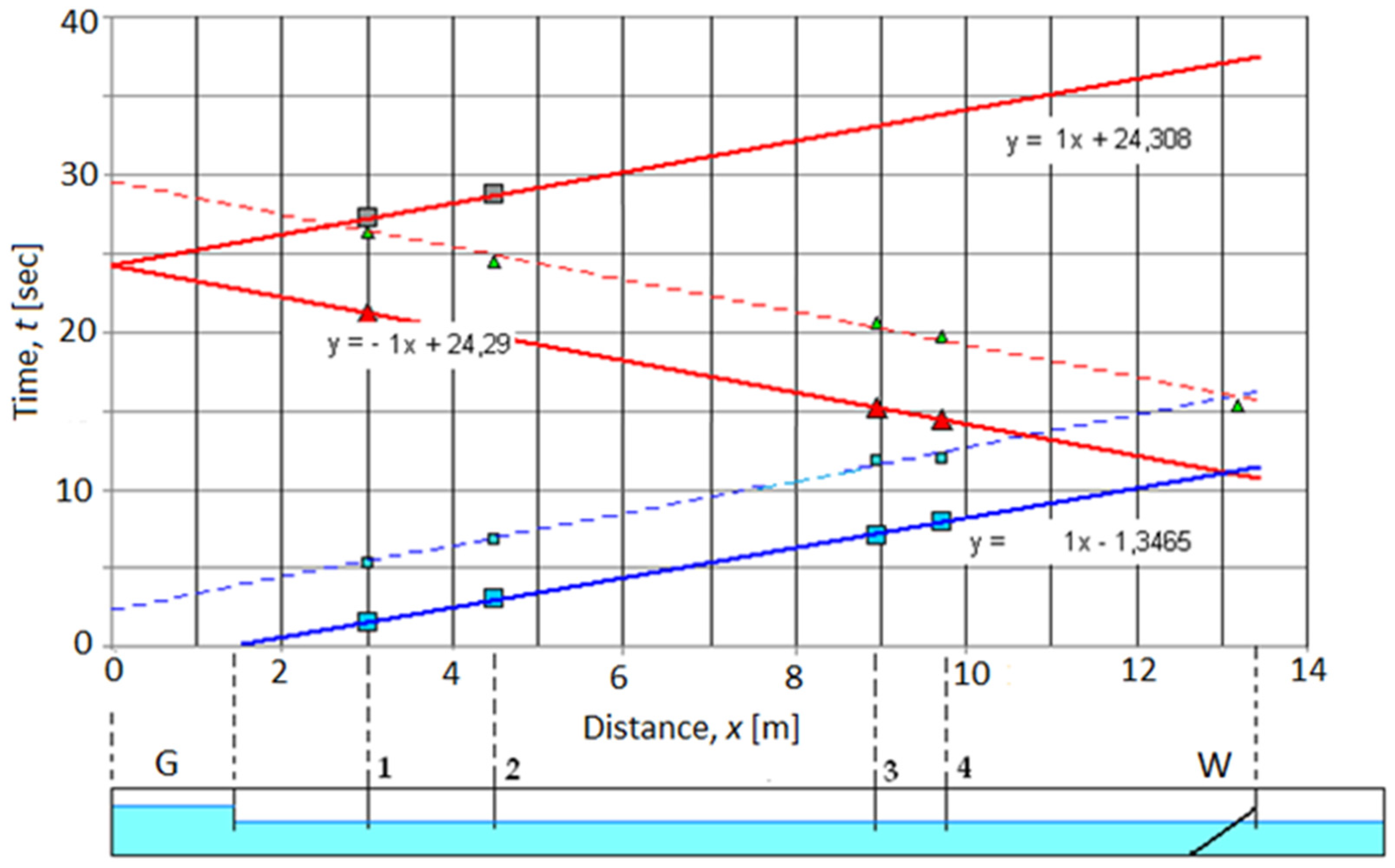
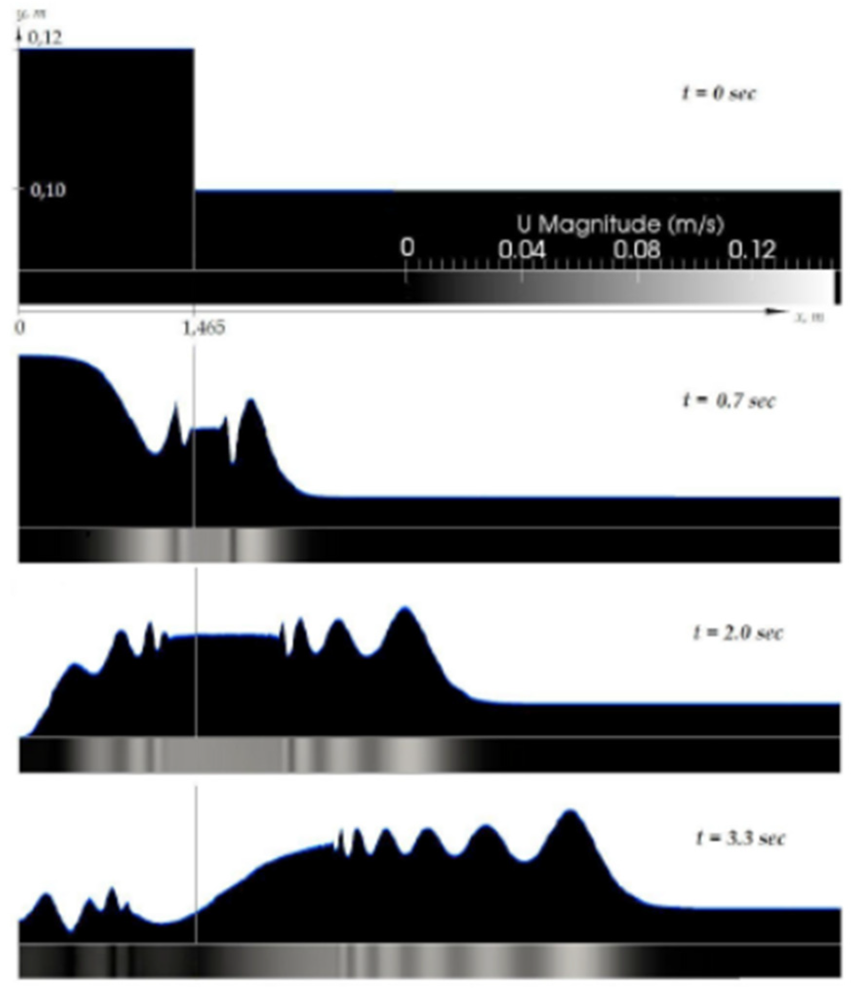
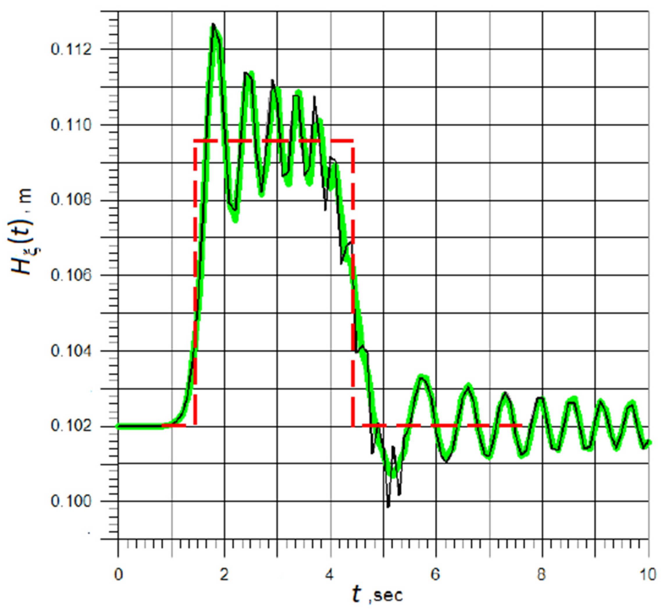
5.2. Wave Propagation

Figure 7 shows a typical x-t diagram of gravity tsunami-like waves, which propagate in the channel. At the bottom (below the diagram) schematic drawing of the channel and locations (1–4) of the sensors are shown in the same scale for the coordinate x. The markers on the diagram show the time of arrival of the waves (incident and reflected), which are registered by each of the four level sensors (see Figure A1 of the Appendix A). Parameters of the experiment: η0 = 15 mm, H = 102 mm.
We can see that the velocities of the incident and reflected waves are equal, c = 1 m/s, and are consistent with the velocity, which was calculated using the linear theory of shallow water c = g H for channel depth H = 0.102 m. The nonlinearity parameter calculated by the average height of the incident wave is equal to A/H = 0.074. Velocities of the waves, which propagate in the channel (solid and dashed lines), calculated by a numerical simulation software based on full Navier—Stokes equations, practically coincided with the measured experimental values (see dots).
Figure 8 shows a comparison of the experimental dependence of the dimensionless wave velocity on the nonlinearity parameter A/H with numerical simulation (2) on the basis of the complete Navier–Stokes Equations. Additionally, theoretical dependencies are shown: dotted line (1)—dependence calculated based on the linear theory of shallow water; and dashed line (3)—calculated by nonlinear shallow-water theory.
It can be seen that the results of numerical simulation (red line) comply best of all with the experimental results (markers). The nonlinear theory of shallow water (1А) provides a qualitatively correct description of the process of wave velocity increase with the growth of nonlinearity parameter but yields an overestimate. Figure 8 shows that the linear theory of shallow water is valid until the nonlinearity parameter exceeds 0.1:
c g H = 1         for       0 < A H < 0.1
The similarity law (6) is important since, in this case, the total energy of a tsunami-type wave can be calculated as the doubled potential wave energy [1] on the basis of the dependence ξ(t) measured by the wave-level sensor:
W = ρ g 0 L ξ 2 ( x ) d x = ρ g g H 0 T ξ 2 ( t ) d t

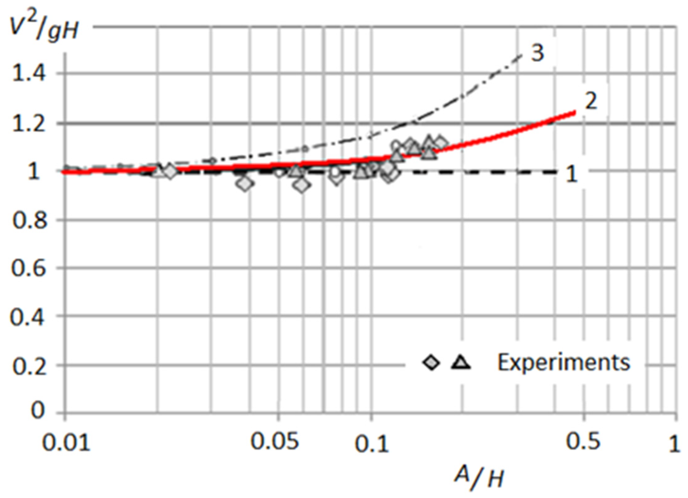
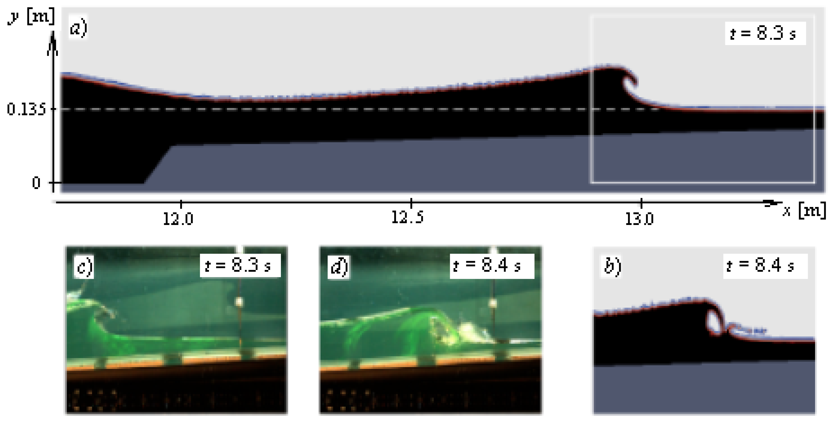
5.3. Transformation of Highly Nonlinear Wave, Which Interacts with Shallow Water

The problem of describing the dynamics of long gravity waves, which propagate in the shallow water of coastal strip causing the flooding of the shore, is one of the most difficult problems concerning the tsunami waves. This is caused by the need to solve the nonstationary problem, as well as by the need to consider nonlinear and viscous effects; that is, in this case, it is necessary to solve the dynamics equations in the most general formulation.
Figure 9 provides a comparison of experimental transformations of strongly nonlinear tsunami-kind waves (1 < A/H < 2, H/L ≈ 0.03) which propagate in the coastal area having gently sloped bottom, with numerical simulation of these processes in the hydrodynamic channel based on the full Navier–Stokes Equations.
Figure 9a in the coordinates x-y (to scale) shows the profile of the shallow part of the bottom (shelf) and the wave profile at the time t = 8.3 s from the beginning of wave initiation in the hydrodynamic channel, which were obtained using numerical simulation. Figure 9c shows a synchronous frame shot by a high-speed camera. The white rectangle indicates the field of view of a high-speed digital camera. Figure 9b,d compare the results of numerical calculation of the waveform with the experiment at the time t = 8.4 s. Figure 9 shows a very good coincidence of numerical simulation results with the experiment. Hence, the proposed mathematical model and its software implementation can be applied to the complex experimental–numerical study of tsunami wave problems in laboratory conditions.

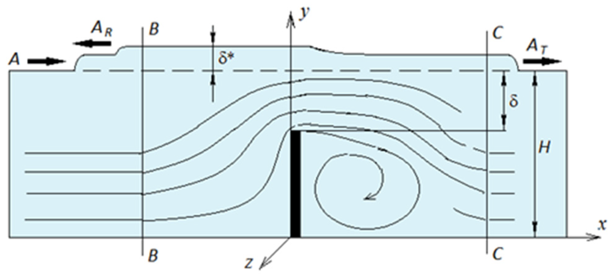
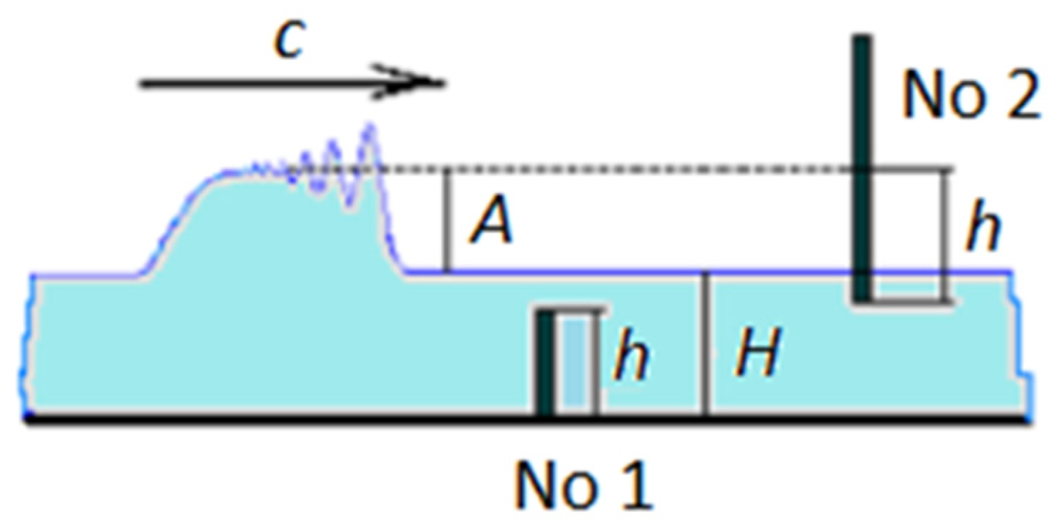
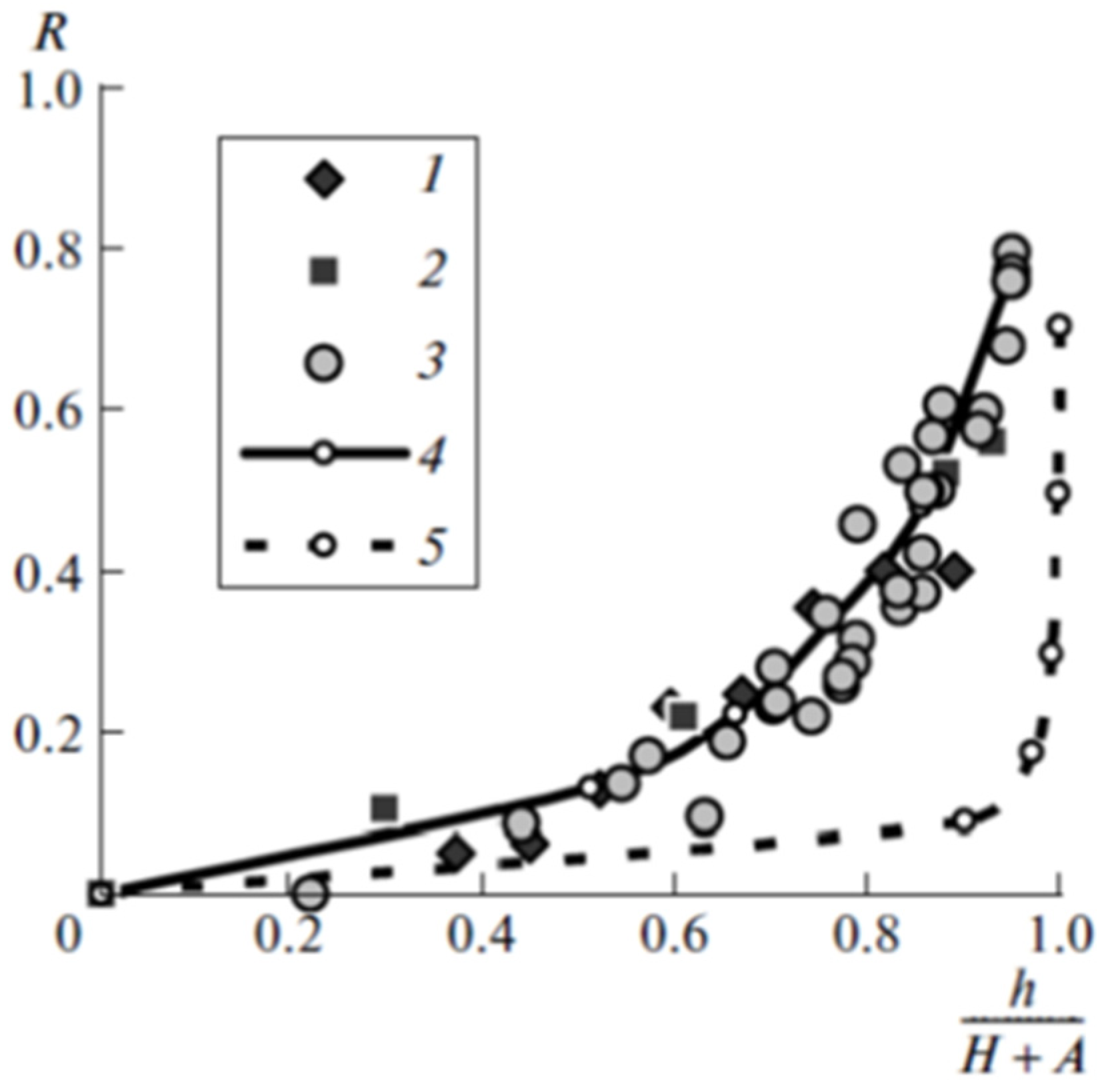
6. Interaction of Tsunami-Like Waves with Impermeable Thin Barriers

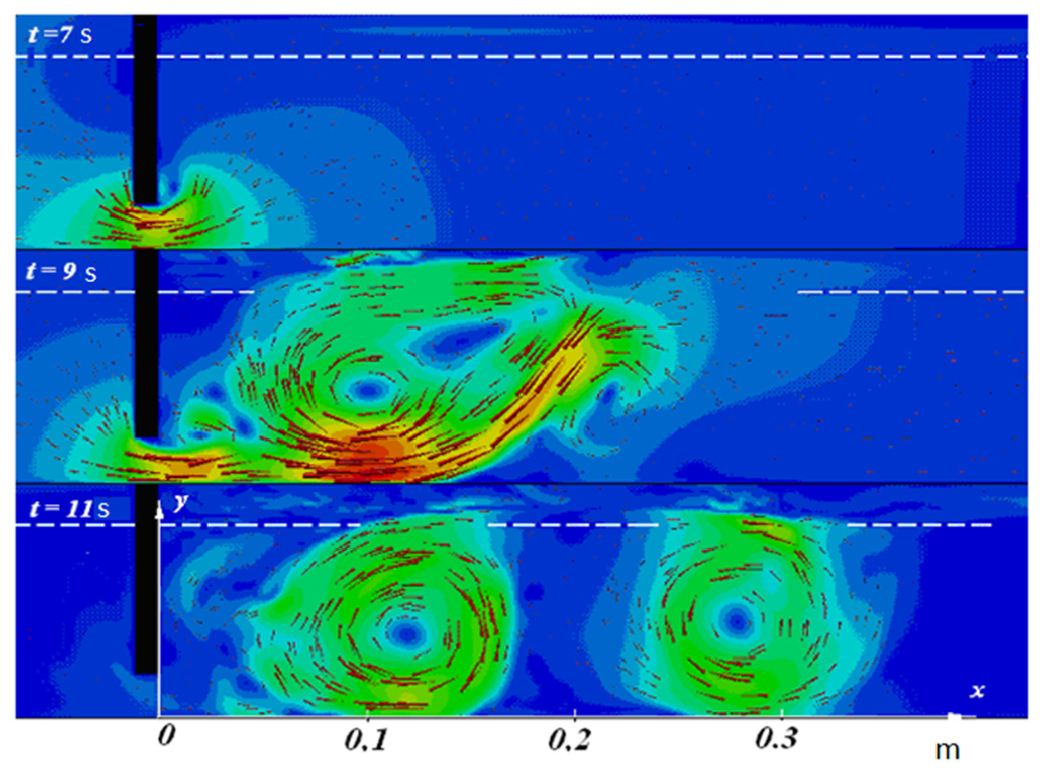
6.1. Experimental and Numerical Studies

A scientific explanation of the effect of anomalous suppression of the energy of tsunami-like waves by two underwater barriers located at a relatively small distance from each other (Δ << L), experimentally discovered by reference [5], was given in the works of the author [8,9].
It turned out that the effectiveness of thin underwater barriers is caused not only by the energy carried away by the wave reflected from the barrier but also by the energy that accumulates near the barrier in large-scale vortex structures. Vortex energy under certain conditions can reach 50% of the energy of the incident wave.
This section presents the results of the investigation regarding tsunami-like waves interacting with impermeable thin barriers of two types (Figure 10).
The barriers have a rectangular shape with thickness 10   mm = δ L , and are installed at a zero angle to the front of the incident wave. Barrier No. 1 was installed at the bottom of the flume, and barrier No. 2 was submerged in the water from above. The height of barrier No. 1 varied in the range 0 < h < (H + A), and the depth of immersion of barrier No. 2 varied in the range 0 < h < H. Our numerous experiments and results of numerical simulations have shown that if ( h H + A ) N o 1 = ( h H + A ) N o 2 , then barriers No. 1 and No. 2 are identical to each other, that is, they equally reduce the energy of the incident wave W: ( W t W ) N o 1 = ( W t W ) N o 2 . However, the use of barrier No. 2 significantly increases the productivity and convenience of experimental studies.
Figure 11 shows the dependence of the amplitude reflection coefficient R = W r / W A r / A on the dimensionless parameter h/(H + A).
It can be seen that all experimental data (with barriers No. 1 and No. 2) are generalized by a single dependence R = f ( h H + A ) in a wide range of variations of the nonlinearity parameter 0.04 < A/H < 0.286. Calculations (dashed line) of the reflection coefficient based on the linear theory of long waves [1] correspond to experiments only in the case when h << (H + A). The results of numerical modeling of the reflection coefficient based on the nonlinear Navier—Stokes Equations in a two-dimensional formulation at A/H = 0.7 (solid line) are also shown in Figure 11. It can be seen that the results of numerical simulation are in very good agreement with the experimental data in the range of variation of the generalized parameter 0 < h/(H + A) < 0.95.
Thus, the linear theory of long waves (or shallow water H << L) is a fairly good approximation for describing the process of propagation of tsunami-type waves in the range of variation of the nonlinearity parameter 0 < A/H < 0.1 (see Figure 8). However, the calculation of the reflection coefficient of waves using the linear theory of long waves gives a strongly underestimated result even for weak (linear) waves at A/H ≈ 0.05 (see Figure 11). So, for example, at a barrier height of h = 0.8 (H + A), the linear theory underestimates the result by a factor of 4 in comparison with the experiment. On the other hand, it would seem that the conditions for linearization of the Navier–Stokes Equations are strictly fulfilled.
We will find an even greater discrepancy with our expectations when we compare the energy characteristics of the incident, reflected, and transmitted waves. Since the viscous losses (from friction) on thin impenetrable barriers are negligible, it is natural to assume that the result of the linear theory of long waves is correct, then W = Wr + Wt.
Figure 12 shows (dark markers) the experimental dependence W r + W t W = f ( h H + A ) for small amplitude tsunami-type waves. The experiments were carried out under the following conditions: water depth H = 0.103 m, the nonlinearity parameter varied in the range 0.04 < A/H < 0.1. The wave energy was calculated by Formula (7) by integrating the experimental dependence of the wave height on time ξ(t).
It is seen that the linear theory of long waves adequately describes the interaction of tsunami-type waves with a thin barrier only if the relative barrier height is less than 0.3(H + А). In the range of barrier heights from 0.3(H + А) to H + 2A, all experiments correspond to the inequality (Wr + Wt) < W. For example, at = 0.9H, experiments show that Wr + Wt ≈ 0.5W. A legitimate question arises: “Where did 50% of the incident wave energy go?” On the other hand, numerical simulation of the experimental conditions based on the full Navier–Stokes Equations (white markers in Figure 12) gives the correct result that coincides with the experiment.
The author proposed a hypothesis that the missing energy is accumulated in large-scale vortex structures near a thin barrier. More studies that are detailed have fully confirmed the correctness of this hypothesis. Later, the author proposed a theory (see Section 6.2), which made it possible to obtain analytical dependences for the reflection and transmission coefficients of tsunami-type waves when they interact with thin underwater barriers, taking into account the vortex effects described above.
A visual picture of the velocity fields during the passage of a tsunami-type wave through a thin barrier at different times is given in Figure 13. These velocity fields were obtained as a result of a numerical experiment based on two-dimensional Navier–Stokes Equations under the condition of maximum energy losses (see Figure 11): H = 0.103 m, L ≈ 3 m, A/H = 0.07, and h/H + A = 0.9.
In Figure 13, a thin barrier No. 2 (shown in black) is installed at a distance of 7 m from the wave generator, and the wave speed is c = 1 m/s. After 7 s from the beginning of wave generation (t = 7 s), the leading front of the wave has already crossed the obstacle, and we see a symmetric picture of the beginning of the interaction between the wave and the barrier. The end of the interaction of the wave with the barrier is shown in 2 s (t = 9 s). We see how the directed energy of the wave is pumped into a large-scale vortex structure stationary relative to the barrier, the diameter of which exceeds the depth of the water. At t = 11 s, the wave passed the obstacle, the trailing front of the wave is approximately 1 m from the barrier, but two practically immobile vortices with a diameter equal to the water depth H remained near the barrier. These vortices contain “the missing 50% of the incident wave energy.
Thus, after interacting with the barrier, the wave lost almost 85% of its energy: 35% of its energy was reflected from the barrier (see Figure 11), and 50% was accumulated in vortex structures near the obstacle. For comparison, note that permeable barriers [4], in which the dissipation of wave energy occurs due to friction, at the same height of the barrier, in total suppress no more than 35% (including 30% in the reflected wave).
If we assume that friction losses in thin impenetrable barriers are negligible, then the energy conservation law will have the following form:
W r + W t W + W v W = 1
where W v W is the relative energy accumulated in large-scale vortex structures near an underwater obstacle.

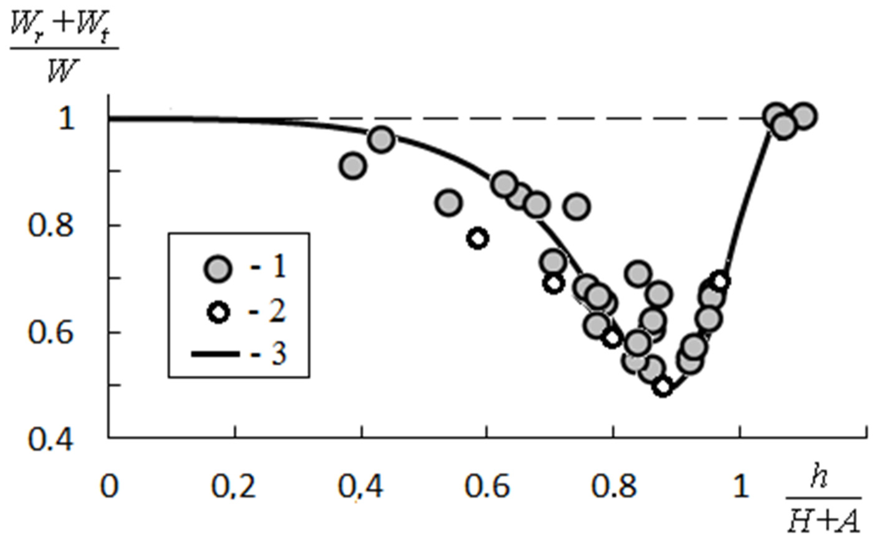
6.2. Theoretical Studies

Experimental and numerical studies presented in Section 6.1 have shown that, under certain optimal conditions, the efficiency of thin and impenetrable underwater barriers can be substantially (more than doubled) increased due to additional energy losses of tsunami waves in large-scale vortex structures. In this section of our review, a theory is given that, in an analytical form, makes it possible to evaluate the efficiency of such underwater barriers with allowance for eddy losses.
Let us consider the problem of the interaction of a tsunami-type wave with a thin and impenetrable underwater barrier in the one-dimensional (along the x-axis) formulation of the “shallow-water theory” (see Figure 14). For this, we temporarily exclude from consideration the region x: (−L/2 < x < +L/2), in which the flow is two-dimensional, and the “shallow water” assumption is not met. In Figure 14, this region is between the cross-sections B—B and C—C (of unit thickness along the coordinate axis z).
It is known that the shallow-water theory describes with sufficient accuracy the propagation of weak tsunami-type waves (A << H) in a reservoir with a smooth change in depth. In this case, the speed of the wave is c = g H , and the total energy of the wave is W = Wk + Wp = 2Wp. Here Wk and Wp are the kinetic and potential energy of the wave. For example, the energy flux through the channel cross-section C—C (Figure 14) is:
q c c = ρ c ( g A t 2 2 + v t 2 2 H ) = ρ c g A t 2
where v t is the depth-averaged fluid velocity behind the front of the transmitted wave.
Let us write down the conditions for the conservation of stationary flows of mass and energy through the cross-sections B—B and C—C, see (А3):
A c = A r c + A t c
ρ g A 2 c = ρ g A r 2 c + ρ g A t 2 c + P
where P is the energy loss due to the barrier per unit time.
Since the main energy losses take place in the region from the barrier to the C—C cross section, the energy loss P can be estimated as hydraulic losses on a sharp expansion of the channel cross-section (“shock” decrease in the flow velocity): above the obstacle, the flow velocity is equal to U, behind the front waves—vt. To do this, we use the Borda–Carnot principle [17], according to which these losses are similar to the energy losses during the inelastic impact of solid balls when one ball catches up with another, which moves at a slower speed. In this case, “the lost kinetic energy is equal to the energy of the lost velocities.” In our case, we have:
P = 1 k 1 + k ρ ( U v t ) 2 2 H c
where 0 < k < 1 is the coefficient of restitution: with k = 0, the impact is perfectly inelastic; and with k = 1, the impact is perfectly elastic.
The velocity over the barrier U as a function of the velocity vt can be easily obtained from the condition of conservation of the liquid flow rate U ( δ + δ * ) = v t H . In our approximation, we have A t H 0.1 and v t 2 2 = g A t 2 2 . Finally, we arrive at Equations (10) and (11) in the form:
1 = R + T ;           1 R 2 = T 2 [ 1 + 0.5 1 k 1 + k ( H δ + δ * 1 ) 2 ]
For T ≠ 0, the formulas:
T = 4 4 + K ;   R = K 4 + K   ;   K = 1 k 1 + k ( h δ * δ + δ * ) 2
give solutions to Equation (13).
In Equation (14), δ* and k are unknown quantities. δ* is the excess of the water level over the initial level H directly above the barrier at the time when the reflected wave is formed: at the full reflection of the wave from the barrier (R = 1), δ* = 2A, and at T = 1 we have δ* = A. For weak waves of the tsunami type (A < 0.1∙H), we can assume with sufficient accuracy that δ* = A. The coefficient of restitution k characterizes the fraction of energy that is converted into heat due to viscosity in small-scale structures of a liquid, and it must be found from experiments.
The result of the calculation according to the proposed theory of energy losses of tsunami-type waves during their interaction with thin impenetrable barriers (solid line) is shown in Figure 12. It is seen that formulas (14) describe, quite accurately, the experimental effect of anomalous suppression of the energy of tsunami-type waves by thin impenetrable barriers. It is important to note that in the range of optimal barrier heights of 0.8 < h/(H + A) < 1, the theoretical calculations almost exactly coincide (see white markers) with the results of numerical modeling based on the full Navier–Stokes Equations.
Note that the best agreement between theory and experiments is achieved at a sufficiently large recovery coefficient k = 0.68. This indicates that most of the kinetic energy of the wave is not absorbed due to viscous friction but accumulates in large-scale vortex structures.

7. Conclusions

This paper includes some results of studies of tsunami wave problems aimed at reducing their destructive power, which were obtained at the Institute Applied Mechanics of the Russian Academy of Sciences in the period from 2013–2019, namely:
  • Investigation of the features of modeling tsunami waves in a laboratory installation;
  • Theoretical, experimental, and numerical studies of the interaction of tsunami waves with underwater obstacles;
  • It is shown that at a certain optimal height of a thin impermeable barrier, its effectiveness in suppressing the energy of an incident tsunami wave is 70%, which is explained by the accumulation of energy in large-scale vortex structures near the obstacle.
We note several important circumstances characteristic of our research:
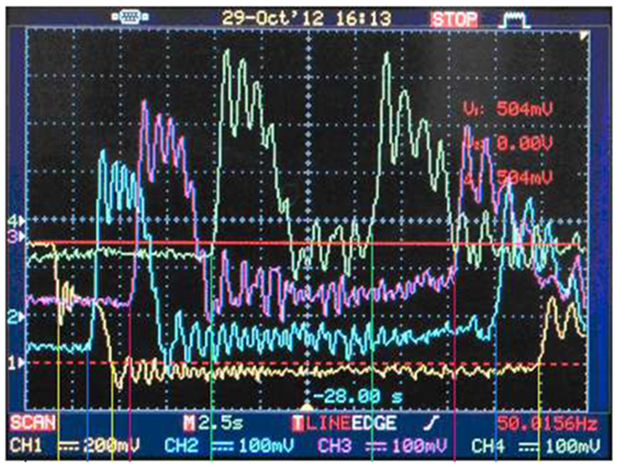
  • The use of precision measuring channels (sensor + equipment) for recording the water level made it possible to simulate the main dimensionless parameters of tsunami waves in a laboratory setup, equivalent to the parameters in large-scale wave flumes;
  • The wave generator ensures the creation of gravity waves equivalent to theoretical ones with an instantaneous jump in water level and speed at the leading edge of the wave. In this case, the wavelength does not depend on its height and is determined only by the length of the wave generator;
  • In our studies, we studied the interaction of a stationary homogeneous water flow u x = A H g H with underwater barriers, since the condition τs < T is always provided, where τs is the time of the establishment of a stationary flow around.
The content of this work is limited to the study of interactions with single underwater barriers of only weak (linear) gravity waves (А/Н ≤ 0.15). At the same time, the reliability of all conclusions increases, so it is possible to apply an integrated approach (theory, experiment, and numerical simulation). In addition, the paper studied flows at Re ≤ 1.5 × 10⁴, i.e., only laminar flows behind the wave front are considered. We do not consider the important problem of modeling the flow around underwater barriers in terms of the dimensionless number Re.
This paper did not include less important results on studies of the interaction of tsunami waves with an underwater barrier of finite thickness and with a complex of two barriers, which are contained in references [8,18,19,20]. In our paper [20], a more detailed review of the problem under study and a comparison of our results with experiments and numerical calculations of other authors are given.
The paper shows that there is a unique opportunity to significantly reduce the destructive power of tsunami waves using the own energy of tsunami waves. We hope that the results of our research can serve as a scientific basis for creating highly effective underwater barriers for tsunami waves.

Funding

This research was funded by the Ministry of Science and Higher Education of the Russian Federation (state order No. 121112200122-7).

Institutional Review Board Statement

Not applicable.

Informed Consent Statement

Not applicable.

Data Availability Statement

Not applicable.

Acknowledgments

I am grateful to Academician É.E. Son for some useful comments. I am also grateful to D.G. Lisin for his help in numerical work.

Conflicts of Interest

The author declares no conflict of interest.

Appendix A. Characteristics of Gravity Waves of the Tsunami Type, Modeled in the Hydrodynamic Channel of the IPRIM RAS

Figure A1 shows a typical oscillogram obtained by recording tsunami-type waves in a hydrodynamic flume with four water level sensors.
Figure A1. A typical oscillogram of tsunami-type wave registration in a hydrodynamic channel.
Geohazards 03 00007 g0a1
Label 1 shows the initial position of the measuring channel of sensor No.1 (yellow), which measures the water level in the wave generator. An increase in the water level in the generator before wave generation by η0 = 0.02 m corresponds to an upward shift of the beam by 491.4 mV. The sensor registered a sharp drop in the water level by −240 mV after the start of the wave generator. This level drop corresponds to a wave that propagates inside the generator and has a height of 𝐴 = − η0/2 with a measurement error of δ = 2.32%. Sensors No. 2–4 (blue and cyan) register waves in the working part of the wave tray. The distance between sensors No.2 and No.4 is 6.7 m. It can be seen from the 546 oscillogram that the time it takes the wave to cover this distance is Δt = 6.56 s. Thus, the experimentally measured wave speed is c = 1.03 m/s. The group velocity of such a single wave calculated on the basis of the linear theory of shallow water is c = g H = 1.001   m / s . From Figure A1, it can be seen that the wave that propagates into the working channel of the flume has a time extension of about T ≈ 3 s, thus: L = 2a = cT ≈ 3 m.
The shape (profile) of the waves generated by our wave generator is completely similar to a real tsunami wave 100 km from an underwater source in the form of a vertical displacement of an extended area of the ocean floor with a residual displacement [21]. If we average the fluctuations that arise due to a sharp change in the water level, then the cross section of these waves along the direction of its propagation will have the form of a trapezoid. Such a wave profile fully corresponds to the calculations of gravity waves arising from the vertical displacement of an extended bottom area of Δx = 2a to a height of η0 in time τ [1]. In this case, if τ * = τ T = 2 a g H 1 , then the average wave height A = η 0 /2, wavelength L = a ( 2 + τ * ) , and the potential energy of the wave is equal to its kinetic energy Wp = Wk. The total wave energy (per meter of length along the front) was calculated using Formula (7) and is equal to W = 2 a ϱ g η 0 2 ( 1 2 τ * 12 )   , where 2 a ϱ g η 0 2 is the potential energy of the area (2a∙1 m2) of water as it rises to a height η0 above the initial level of the liquid.
In our case, there are no moving parts in the wave generator, so we can assume that τ* = 0. Then the calculated profile of the generated wave in the approximation of the linear theory of shallow water will have a rectangular shape: L = 2a, A = η0/2. In Figure 5, the red line shows the profile of such a model wave. The potential energy of the model wave, as expected, is equal to half of the initial potential energy of the generator: W p = 2 ρ g a ( η 0 2 ) 2 = 1 2 ρ g a η 0 2 . The calculation of the potential energy of real waves by integrating the experimental wave profile using the Formula W p = 1 2 ϱ g g H 0 T ξ ( t ) d t gives the same result.
Let us estimate from Figure 5 the maximum vertical velocity of the liquid, which is given by oscillations on the crest of the wave: u z = A v 2 π T v = 0.0025 2 π 2 = 0.008   m / s . Horizontal flow velocity behind the wave front is u x = A H g H 0.1   m / s . Thus, in our experiments, the oscillations that arise at the crest of the wave practically do not distort the velocity profile uniform over the entire depth behind the wave front. Figure A2 shows the process of generating a model wave.
Figure A2. The process of generating a model wave by a caisson-type generator.
Geohazards 03 00007 g0a2
At time t = 0, there is a given level difference in the wave generator and in the working channel, and the fluid velocity is zero everywhere. For t > 0, the given arbitrary discontinuity of levels splits into two waves. At t = t1, the wave А1 = −η0/2 moves inside the generator, and the wave А2 = η0/2 moves into the working channel. At t = t2, wave A1 is reflected from the wall and, together with wave A2, forms a single wave of length L = 2a, which moves into the working channel (see t = t3).
Thus, the model gravity wave (see Figure 5), which is used in the theoretical estimates of Section 6.2 of this work, models our real wave in a hydrodynamic flume with high accuracy. This wave propagates through the shallow water of the flume (L >> H) with a constant speed c = g H as a small perturbation (A << H). The trailing and leading wave fronts are discontinuity surfaces that move in the same direction with a constant depth velocity uv = c. Before the wave and behind the rear surface of the discontinuity, the water velocity is zero. The fluid velocity inside the wave is u << c; it (like the velocity c) does not depend on spatial coordinates y-z. A schematic drawing of the wave in a fixed (laboratory) frame of reference is shown in Figure A3a.
Figure A3. Schematic drawing of the motion of a gravitational wave in various frames of reference: (a) in a fixed (laboratory) frame of reference; (b) in a moving (with the speed of a wave) frame of reference.
Geohazards 03 00007 g0a3
For the mathematical description of such waves, continuous functions and differential equations are inapplicable (for example, on the discontinuity surface divU = ∞). However, the relationship between the wave parameters can be obtained from the conditions of mass and momentum flux conservation on both sides of the discontinuity. Since the wave propagates in one direction without changing its shape, then, passing into a moving (with speed c) frame of reference, we turn the nonstationary problem into a stationary one. In this frame of reference (Figure A3b), the conservation conditions have the form [22]:
u 1 h 1 = u 2 h 2
u 1 2 h 1 + g h 1 2 2 = u 2 2 h 2 + g h 2 2 2
The notation in Formulas (A1) and (A2) is clear from Figure A3. From Equation (A1), we obtain a formula for calculating the mass flux density (referred to 1 m of the channel width), which is carried by the model wave:
j = u ( H + A ) = c A
The speed of a nonlinear wave u1, with an arbitrary value of the nonlinearity parameter ε = A/H, is also easy to obtain from relations Equations (A1) and (A2):
u 1 2 = g H ( 1 + ε 2 ) ( 1 + ε )
Note that, in the general case, the energy fluxes on both sides of the discontinuity are not the same, i.e., due to the sharp expansion of the flow, there are energy losses. However, in our case, for ε << 1, the energy fluxes are equal to within O2).
Thus, long gravity waves of the tsunami type, modeled in our wave tray, as well as natural tsunami waves, are displacement waves, in which the mass of liquid and energy is transferred in the direction of wave movement. This is precisely why real tsunami waves fundamentally differ from progressive oscillatory waves in which the average fluid flow rate is zero. The second feature of natural tsunami waves is that, due to their exceptionally large length, the interaction of tsunamis with protective barriers and coastal structures occurs almost under stationary conditions. Noncompliance with the latter condition when conducting studies in ground-based facilities (wave flumes) can lead to gross errors [7,14]. A distinctive feature of our waves is that we have a practically uniform and stationary fluid flow behind the wave front for a rather long time T. The latter circumstance is very important since the time for establishing a stationary flow around underwater barriers can be more than 10 H g H seconds.

References

  1. Levin, B.W.; Nosov, M.A. Physics of Tsunamis, 2nd ed.; Springer: Cham, Switzerland, 2016; p. 388. [Google Scholar] [CrossRef]
  2. Shokin, Y.I.; Chubarov, L.B.; Marchuk, A.G.; Simonov, K.V. Vychislitelnyy Eksperiment v Probleme Tsunami. In Computational Experiment in the Tsunami Problem; Nauka SB: Novosibirsk, Russia, 1989. (In Russia) [Google Scholar]
  3. Ton van der Plas, T. A Study into the Feasibility of Tsunami Protection Structures for Banda Aceh and a Pre-Liminary Design of an Offshore Rubblemound Tsunami Barrier; Final Thesis Report; Delft University of Technology: Amersfoort, The Netherlands, 2007; pp. 1–24. [Google Scholar]
  4. Irtem, E.; Seyfioglu, E.; Kabdasli, S. Experimental investigation on the effects of submerged breakwaters on tsunami run-up height. J. Coast. Res. 2011, 64, 516–520. [Google Scholar]
  5. Fridman, A.M.; Alperovich, L.S.; Pustilnic, L.; Shemer, L.; Marchuk, A.G.; Liberson, D. Tsunami wave suppression using submarine barriers. Physics-Uspekhi 2010, 53, 809–816. [Google Scholar] [CrossRef]
  6. Boshenyatov, B.V.; Popov, V.V. Eksperimental’nye issledovaniya vzaimodeystviya voln tipa tsunami s podvodnymi pregradami [Experimental studies of the interaction of tsunami-like waves and underwater obstacles]. Izv. Vyss. Uchebnyh Zaved. Phisika 2012, 55, 145–150. (In Russia) [Google Scholar]
  7. Madsen, P.A.; Fuhrman, D.R.; Schaffer, H.A. On the solitary wave paradigm for tsunamis. J. Geophys. Res. 2008, 113, 1–22. [Google Scholar] [CrossRef]
  8. Boshenyatov, B.V.; Zhil’tsov, K.N. Matematicheskoye modelirovaniye vzaimodeystviya dlinnykh voln tipa tsunami s kompleksom pregrad [Mathematical simulation of the interaction of long tsunami type waves and complex of barriers]. Mod. High Technol. 2015, 12, 20–23. (In Russia) [Google Scholar]
  9. Boshenyatov, B.V. The vortex mechanism of suppression of tsunami waves by underwater obstacles. Dokl. Earth Sci. 2017, 447, 1434–1436. [Google Scholar] [CrossRef]
  10. Qu, К.; Ren, X.Y.; Kraatz, S. Numerical investigation of tsunami-like wave hydrodynamic characteristics and its comparison with solitary wave. Appl. Ocean. Res. 2017, 63, 36–48. [Google Scholar] [CrossRef]
  11. Shemer, L.; Goulitski, K.; Kit, E. Evolution of wide-spectrum unidirectional wave groups in a tank: An experimental and numerical study. Eur. J. Mech. B/Fluids 2007, 26, 193–219. [Google Scholar] [CrossRef]
  12. Boshenyatov, B.V.; Levin, Y.K.; Popov, V.V. Ustroystvo izmereniya urovnya vody [Water level measuring device]. RF Patent Application No. 2485452, 10 July 2010. [Google Scholar]
  13. Kutateladze, S.S.; Mironov, B.P.; Nakoryakov, V.E.; Habahpasheva, E.M. An Experimental Study of Wall Turbulent Flows; Nauka: Novosibirsk, Russia, 1975; pp. 23–30. (In Russia) [Google Scholar]
  14. Hirt, C.W.; Nichols, B.D. Volume of fluid (VOF) method for the dynamics of free Boundaries. J. Comp. Phys. 1981, 39, 201. [Google Scholar] [CrossRef]
  15. OpenFOAM Foundation. OpenFOAM. In User Guide; OpenFOAM Foundation: London, UK, 2016; p. 211. Available online: http://www.openfoam.org (accessed on 15 March 2018).
  16. Boshenyatov, B.V.; Lisin, D.G. Numerical simulation of tsunami type waves in a hydrodynamic channel. Vestn. Tomsk. Gos. Universiteta. Mat. I Mekhanika [Tomsk. State Univ. J. Math. Mech.] 2013, 6, 45–55. [Google Scholar]
  17. Zhukovskii, N.E. Theoretical Foundations of Aeronautics; Gostekhizdat: Moscow, Russia, 1925. (In Russian) [Google Scholar]
  18. Boshenyatov, B.V.; Zhiltsov, K.N. Simulation of the interaction of tsunami waves with underwater barriers. Am. Inst. Phys. Conf. Ser. 2016, 1770, 030088. [Google Scholar] [CrossRef]
  19. Boshenyatov, B.V.; Zhil’tsov, K.N. Investigation of the interaction of tsunami waves and submerged obstacles of finite thickness in a hydrodynamic wave flume. Vestn. Tomsk. Gos. Universiteta. Mat. I Mekhanika [Tomsk. State Univ. J. Math. Mech.] 2018, 51, 86–103. (In Russia) [Google Scholar] [CrossRef] [PubMed] [Green Version]
  20. Boshenyatov, B.V.; Zhil’tsov, K.N. Vortex suppression of tsunami-like waves by underwater barriers. Ocean. Eng. 2019, 183, 398–408. [Google Scholar] [CrossRef]
  21. Chierici, F.; Pignagnoli, L.; Embriaco, D. Modeling of the hydroacoustic signal and tsunami wave generated by seafloor motion including a porous seabed. J. Geophys. Res. Ocean. 2010, 115, C0315. [Google Scholar] [CrossRef] [Green Version]
  22. Landau, L.D.; Lifshitz, E.M. Fluid Mechanics, 2nd ed.; Nauka: Moscow, Rassia; Pergamon Press: Oxford, UK, 1987. [Google Scholar]
Figure 1. The hydrodynamic channel (wave flume) of the IPRIM RAS.
Geohazards 03 00007 g001
Figure 2. Calibration stand and equipment.
Geohazards 03 00007 g002
Figure 3. Тypical calibration curve. (a) Schematic diagram of the resistive sensor.
Geohazards 03 00007 g003
Figure 4. Schematic drawing of the caisson-type generator.
Geohazards 03 00007 g004
Figure 5. Modeling the process of generating a tsunami-type wave in a wave flume by an ideal generator at H = 0.103 m, A/H = 0.1.
Geohazards 03 00007 g005
Figure 6. Comparison of experimental dependence wave height—time (green line) ξ(t) = Hξ(t) − H with the numerical calculation for ideal generator (black line) at a distance of 1.5 m from the front wall of wave generator. The red dashed line is the model wave profile.
Geohazards 03 00007 g006
Figure 7. The diagram (x-t) of gravity tsunami-like waves, which propagate in the hydrodynamic channel at the following initial parameters: η0 = 15 mm, H = 102 mm, A/H = 0.074. Makers—experiments. Lines—linear theory of shallow water. The blue line is the trajectory of the incident wave; the red lines are the reflected waves. G—wave generator; W—reflecting wall; 1–4—locations of wave level sensors.
Geohazards 03 00007 g007
Figure 8. Dependence of long gravity waves velocity in the hydrodynamic channel on the nonlinearity parameter A/H: 1—linear theory of shallow water, 2—Navier–Stokes Equations, 3—nonlinear theory of shallow water (4А).
Geohazards 03 00007 g008
Figure 9. Breaking of wave interacting with shallow water. The comparison of experimental results with numerical simulation at H = 0.135 m, A/H = 0.61, Hsh = 0.054 m, A/Hsh = 1.52: (a,c)—t = 8.3 s; (b,d)—t = 8.4 s.
Geohazards 03 00007 g009
Figure 10. Schematic diagram of the interaction of a tsunami-type wave with impenetrable barriers No. 1 and No. 2.
Geohazards 03 00007 g010
Figure 11. Reflection coefficient as a function of dimensionless parameter h/(H + A): (1)—No. 1, A/H = 0.286 [4]; (2)—No. 1, A/H = 0.04–0.05; (3)—No. 2, A/H = 0.04–0.10; (4)—Navier–Stokes Equations, A/H = 0.07 and (5)—linear theory of long waves.
Geohazards 03 00007 g011
Figure 12. The sum of the relative energies of the waves reflected and transmitted through the barrier as a function of the generalized parameter of the barrier height: 1—experiments; 2—numerical experiment based on f Equations; 3—calculations by author’s theory at Н = 0.103 m, А = 0.007 m, and k = 0.68.
Geohazards 03 00007 g012
Figure 13. Visualization for various instants of time of velocity fields near thin barrier No. 2 (black color) in the case of transmission through it of a tsunami type wave: A/H = 0.07, parameter h/(H + A) = 0.9. The dashed line corresponds to the unperturbed water flow level.
Geohazards 03 00007 g013
Figure 14. Schematic diagram of the interaction of a tsunami-type wave with a thin impenetrable barrier. Shallow water theory is not applicable near the barrier: −L/2 < x < +L/2.
Geohazards 03 00007 g014
Table 1. Estimated parameters of tsunami waves for the most realistic underwater earthquakes.
ZoneWater Depth,
H (km)
Wave Height
A (m)
Wave Length
L (km)
Nonlinearity
A/H
Dispersion
H/L
Ocean414000.000250.01
Continental shelf0.1502.25800.0150.0019
Shallow0.0154300.270.0005
Publisher’s Note: MDPI stays neutral with regard to jurisdictional claims in published maps and institutional affiliations.

